Formation Control for UAV-USVs Heterogeneous System with Collision Avoidance Performance

Abstract

This paper investigates the cooperative formation trajectory tracking problem for heterogeneous unmanned aerial vehicle (UAV) and multiple unmanned surface vessel (USV) systems with collision avoidance performance. Firstly, a formation control protocol based on extended state observer (ESO) is proposed to ensure that the UAV and the USVs track the target trajectory simultaneously in the XY plane. Then, the collision avoidance control strategy of USV formation based on artificial potential field (APF) theory is designed. Specifically, the APF method is improved by reconstructing the repulsive potential field to make the collision avoidance action of USVs more in line with the requirements of International Regulations for Preventing Collisions at Sea (COLREGs). Following that, an altitude controller for the UAV is proposed to maintain the cooperative formation of the heterogeneous systems. Based on the input-to-state stability, the stability of the proposed control structure is proven, and all the signals in the closed-loop system are ultimately bounded. Finally, a simulation study is provided to show the efficacy of the proposed strategy.

1. Introduction

In the past few years, unmanned systems have gained significant prominence in the realm of industrial advancement, attributed to their diverse usage in areas such as reconnaissance [1,2], marine pollution tracking [3,4], and advanced traffic management [5,6]. These systems principally encompass unmanned aerial vehicles (UAVs), unmanned ground vehicles (UGVs), unmanned surface vehicles (USVs), and autonomous underwater vehicles (AUVs) [7,8]. Although each unmanned system can handle tasks, its capacity limits its ability to deal with more complex tasks. Therefore, a homogeneous or heterogeneous system is more effective than a single unmanned system in completing intricate tasks [9,10,11].

The development of USV has been widely employed in ocean engineering due to its benefits, which include increased loading capacity, more convenience, and cheaper mission costs [12,13]. However, finding the rescue target in rescue missions and maritime searches is difficult owing to the restricted observation range of USVs [14,15]. Fortunately, incorporating UAVs into USV systems to construct heterogeneous multi-agent systems can compensate for this shortcoming [16,17]. A USV usually boosts its capacity to operate at sea by using the UAV’s flexibility and utilizing the powerful target search ability while simultaneously widening the communication range of the sea between USVs, therefore, the heterogeneous systems extend the effective working area [18,19]. As a result, it is critical to investigate the formation challenges of a heterogeneous system, which has primarily engineering importance.

For the cooperative tracking control problem of UAVs and USVs, many research results have been addressed, among which typical control methods include the leader following method [20], virtual structure method [21], behavior-based approach [22], and model prediction method [23]. In [24], a series of coordinate transformations have been developed to convert the tracking error dynamics of a marine aerial-surface heterogeneous system into translation–rotation cascade forms. This eliminates variability between the UAV and the USV in terms of both translation and rotation dynamics. In [25], the research proposes an adaptive fault-tolerant time-varying formation control scheme. This scheme is particularly tailored to address challenges posed by actuator failures, parameter uncertainties, and external disturbances within the framework of a directed communication topology.

In the area of cooperative control of heterogeneous formations of UAVs and USVs, a globally applicable fixed-duration adaptive neural network is designed in [18] that employs a nonsingular rapid terminal sliding approach for formation control. This protocol is engineered to accurately follow a specified trajectory and achieve a predefined formation arrangement within a set timeframe, effectively addressing a range of uncertainties. This is accomplished by harnessing the combined strengths of adaptive methodologies and Radial Basis Function (RBF) neural networks. In [26], the research proposes a velocity estimation-based control strategy that comprises a distributed observer for estimating each vehicle’s reference velocity. In [23], a distributed model predictive control algorithm tailored for heterogeneous systems is presented, characterized by a directed topological structure.

It is worth noting that the above research results tend to focus on the establishment of air–sea cooperation and the realization of trajectory tracking without considering the problem of collision avoidance [27,28]. During the mission, a minimum safe distance has to be maintained between any two unmanned systems to prevent collisions and to avoid damage to the overall performance of the search and rescue cooperative mission. Therefore, another key issue for the heterogeneous formation system is collision avoidance. Collision avoidance includes not only avoiding collisions between unmanned systems or between unmanned systems and other individuals but also avoiding collisions between unmanned systems and obstacles. Collision avoidance can be further divided into static collision avoidance based on sensor information and dynamic collision avoidance based on an unknown environment. Collision avoidance between aerial vehicles and obstacles can be divided into two ways: overall collision avoidance and changing formation collision avoidance.

There are relatively few research results on the cooperative formation control of heterogeneous systems with collision avoidance and obstacle avoidance. To avoid collision between ships, Refs. [29,30] propose an unmanned ship formation control method based on guaranteed performance, but the collision avoidance of obstacles is not addressed. For the collision avoidance problem between UAVs with static and dynamic obstacles, a cooperative controller for multiple unmanned ships based on artificial potential function is proposed in [12,31], while in the area of cooperative collision avoidance and obstacle avoidance for heterogeneous systems, research results are more limited. In [32], a distributed heterogeneous cooperative tracking control approach is proposed based on the leader-following method, and the artificial potential field (APF) algorithm is used to construct a control strategy with a collision avoidance mechanism. However, the research results between vehicles ignore the nautical engineering practice and poorly consider the COLREGs.

Based on the preceding analysis, this paper investigates the cooperative formation trajectory tracking problem for UAV-USV heterogeneous systems with model uncertainty and external disturbances. To solve this problem, a formation control protocol based on extended state observer (ESO) is proposed to ensure that UAV and USV track the target trajectory simultaneously. The collision avoidance control strategy of USV formation based on improved APF theory is designed. The collision avoidance problem between multiple USV formations formed under UAV coordination is solved by innovatively introducing the ship encounter situation and danger evaluation index into the artificial potential field. The key contributions can be summarized as follows:

(1)

Compared with the existing results in [12,29,30,31], which only study the cooperative trajectory tracking problem of UAV and USV heterogeneous systems, this paper explores the collision avoidance protocol for USV formation under UAV cooperation with navigation practice.

(2)

Compared with the existing results in [18,25,26,32], which estimate that the system’s indeterminate terms rely on RBF neural networks and fuzzy logic, etc., this paper employs ESO to realize the accurate compensation of uncertainties and external disturbances in heterogeneous systems.

(3)

Compared with the existing results in [31,32,33,34,35,36,37], this paper innovatively introduces the ship encounter situation and danger evaluation index into the APF approach, and the improved APF method for heterogeneous cooperative control collision avoidance decision is more in line with the navigation practice.

The organization of this paper is structured as follows. Section 2 formulates the problem. Section 3 expounds on the controller design and the closed-loop system stability analysis. Section 4 demonstrates the simulation illustrations. Section 5 concludes this paper.

2. Preliminaries and Problem Statement

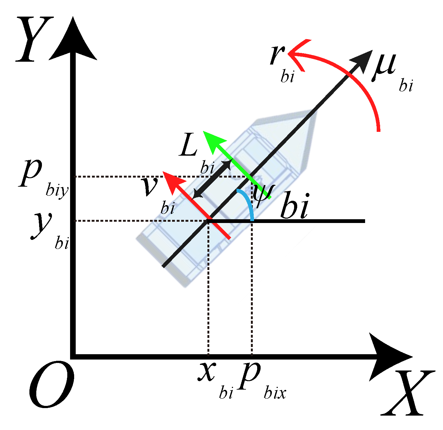
2.1. Problem Formulation

Consider the heterogeneous systems consisting of one UAV and N USVs. First, the dynamic models of the UAV and N USVs are presented. They are used to illustrate a unified dynamic model for the heterogeneous system. For ease of use, let $\mathsf{\Pi }=\{1,2,\dots ,N\}$. According to the results in [38], the dynamic model of the quadrotor UAV can be described as

$$\left\{\begin{array}{c}{\ddot{p}}_{ax}=\left(sin{\varphi }_{a}sin{\psi }_a+cos{\varphi }_{a}sin{\theta }_{a}cos{\psi }_a\right)\frac{u_{ap}}{m_a}-\frac{d_{ax}{\dot{p}}_{ax}}{m_a}+{\Delta }_{ax},\hfill \\ {\ddot{p}}_{ay}=\left(sin{\varphi }_{a}cos{\psi }_a+cos{\varphi }_{a}sin{\theta }_{a}sin{\psi }_a\right)\frac{u_{ap}}{m_a}-\frac{d_{ay}{\dot{p}}_{ay}}{m_a}+{\Delta }_{ay},\hfill \\ {\ddot{p}}_{az}=\left(cos{\theta }_{a}cos{\varphi }_a\right)\frac{u_{ap}}{m_a}-\frac{d_{az}{\dot{p}}_{az}}{m_a}-g_a+{\Delta }_{az},\hfill \end{array}\right.$$

(1)

$$\left\{\begin{array}{c}\ddot{{\varphi }_a}=\dot{{\theta }_a}\dot{{\psi }_a}\frac{J_{ay}-J_{az}}{J_{ax}}-\frac{J_{ar}}{J_{ax}}\dot{{\theta }_a}{\overline{d}}_a+\frac{{\tau }_{a\varphi }}{J_{ax}}-\frac{d_{a\varphi }\dot{{\varphi }_a}}{J_{ax}},\hfill \\ \ddot{{\theta }_a}=\dot{{\varphi }_a}\dot{{\psi }_a}\frac{J_{az}-J_{ax}}{J_{ay}}-\frac{J_{ar}}{J_{ay}}\dot{{\varphi }_a}{\overline{d}}_a+\frac{{\tau }_{a\theta }}{J_{ay}}-\frac{d_{a\theta }\dot{{\theta }_a}}{J_{ay}},\hfill \\ \ddot{{\psi }_a}=\dot{{\varphi }_a}\dot{{\theta }_a}\frac{J_{ax}-J_{ay}}{J_{az}}+\frac{{\tau }_{a\psi }}{J_{az}}-\frac{d_{a\psi }\dot{{\psi }_a}}{J_{az}},\hfill \end{array}\right.$$

(2)

where ${\left[{\varphi }_a,{\theta }_a,{\psi }_a\right]}^T$ is the attitude state, ${\left[p_{ax},p_{ay},p_{az}\right]}^T$ is the position state, ${\tau }_{a\varphi },{\tau }_{a\theta },{\tau }_{a\psi }$ are the three control torques, $u_{ap}$ is the control thrust, $g_a$ is the gravitational acceleration, $m_a$ denotes the mass, ${\overline{d}}_a$ is the overall residual rotor angle, $J_{ax},J_{ay},J_{az}$ represent the moments of the inertia, $d_{ax},d_{ay},d_{az},d_{a\varphi },d_{a\theta },d_{a\psi }$ represent the translational drag coefficients, ${\Delta }_{ax},{\Delta }_{ay},{\Delta }_{az}$ are the external disturbances encountered, and $J_{ar}$ denotes the moment of rotor’s inertia.

Inspired by the results in [25], the UAV’s rotational dynamics can be stabilized separately. Therefore, in light of external disturbances and parametric uncertainties, the UAV model (1) is redefined in the following manner

$${\ddot{p}}_a=g_a{u}_a+f_a+{\Delta }_a$$

(3)

where $p_a={\left[p_{ax},p_{ay},p_{az}\right]}^T$ is the position, $f_a={[-d_{ax}{\dot{p}}_{ax}/m_a,-d_{ay}{\dot{p}}_{ay}/m_a,-d_{az}{\dot{p}}_{az}/m_a-g_a]}^T$, $g_a=diag\left\{1/m_a,1/m_a,1/m_a\right\}$, ${\Delta }_a={\left[{\Delta }_{ax},{\Delta }_{ay},{\Delta }_{az}\right]}^T$, $u_a={\left[u_{ax},u_{ay},u_{az}\right]}^T$ denotes the new control signal which is given as [39]

$$\left\{\begin{array}{c}{u}_{ax}=\left(sin{\varphi }_{a}sin{\psi }_a+cos{\varphi }_{a}sin{\theta }_{a}cos{\psi }_a\right)u_p\hfill \\ u_{\mathrm{ay}}=\left(sin{\varphi }_{a}cos{\psi }_a+cos{\varphi }_{a}sin{\theta }_{a}sin{\psi }_a\right)u_p\hfill \\ u_{az}=\left(cos{\theta }_{a}cos{\varphi }_a\right)u_p\hfill \end{array}\right.$$

In the horizontal plane, the i-th $\left(i\in \mathsf{\Pi }\right)$ USV’s kinematic and dynamic equations are described as [40]

$$\left\{\begin{array}{c}{\dot{x}}_{bi}={\mu }_{bi}cos{\psi }_{bi}-v_{bi}sin{\psi }_{bi},\hfill \\ {\dot{y}}_{bi}={\mu }_{bi}sin{\psi }_{bi}+v_{bi}cos{\psi }_{bi},\hfill \\ {\dot{\psi }}_{bi}=r_{bi}\hfill \end{array}\right.$$

(4)

$$\begin{array}{c}\hfill \left\{\begin{array}{c}{\dot{\mu }}_{bi}=f_{\mu bi}\left({\alpha }_i\right)+\frac{1}{m_{\mu bi}}\left({\tau }_{\mu bi}^f+w_{\mu bi}\right),\hfill \\ {\dot{v}}_{bi}=f_{vbi}\left({\alpha }_i\right)+\frac{1}{m_{vbi}}{w}_{vbi}\hfill \\ {\dot{r}}_{bi}=f_{rbi}\left({\alpha }_i\right)+\frac{1}{m_{rbi}}\left({\tau }_{rbi}^f+w_{rbi}\right)\hfill \end{array}\right.\end{array}$$

(5)

and

$$\left\{\begin{array}{c}{f}_{\mu bi}\left({\alpha }_i\right)=\frac{1}{m_{\mu bi}}\left(m_{vbi}{v}_{bi}{r}_{bi}-d_{\mu bi}{\mu }_{bi}-d_{\mu bi1}\left|{\mu }_{bi}\right|{\mu }_{bi}\right)\hfill \\ f_{vbi}\left({\alpha }_i\right)=\frac{1}{m_{vbi}}\left(-m_{\mu bi}{\mu }_{bi}{r}_{bi}-d_{vbi}{v}_{bi}-d_{vbi1}\left|v_{bi}\right|v_{bi}\right),\hfill \\ f_{rbi}\left({\alpha }_i\right)=\frac{1}{m_{rbi}}\left(\left(m_{\mu bi}-m_{vbi}\right){\mu }_{bi}{v}_{bi}-d_{rbi}{r}_{bi}-d_{rbi1}\left|r_{bi}\right|r_{bi}\right),\hfill \end{array}\right.$$

(6)

where ${\psi }_{bi}$ denotes the yaw angle; $\left(x_{bi},y_{bi}\right)$ denotes the position; ${\alpha }_i={\left[{\mu }_{bi},v_{bi},r_{bi}\right]}^T$ denote the surge, sway, and yaw velocity, respectively; $m_{\mu bi}, m_{vbi}, m_{rbi}$ represent the inertial mass; $f_{\mu bi}\left({\alpha }_i\right)$, $f_{vbi}\left({\alpha }_i\right)$, $f_{rbi}\left({\alpha }_i\right)$ denote the nonlinear dynamics consisting of Coriolis forces and the unmodeled hydrodynamics; $w_{\mu bi}, w_{vbi}, w_{rbi}$ represent the bounded disturbances; and ${\tau }_{\mu bi}^f$ and ${\tau }_{rbi}^f$ represent the surge force and the yaw moment.

Because the USVs’ motion model given in (4) and (5) is underactuated, a hand position technique is employed to compensate. The USVs’ front point $\left(p_{bix},p_{biy}\right)$ is defined as the hand point, which can be expressed as

$$\left\{\begin{array}{c}{p}_{bix}=x_{bi}+L_{bi}cos{\psi }_{bi}\hfill \\ p_{biy}=y_{bi}+L_{bi}sin{\psi }_{bi}\hfill \end{array}\right.$$

(7)

where $L_{bi}$ denotes the distance between the new defined hand point $\left(p_{bix},p_{biy}\right)$ and the actual position $\left(x_{bi},y_{bi}\right)$, which is depicted in Figure 1.

The second derivative of (7) yields the following result

$$\left\{\begin{array}{cc}\hfill {\ddot{p}}_{bix}=& {\dot{\mu }}_{bi}cos{\psi }_{bi}-\left({\dot{v}}_{bi}+L_{bi}{\dot{r}}_{bi}\right)sin{\psi }_{bi}-{\mu }_{si}{r}_{bi}sin{\psi }_{bi}\hfill \\ & -\left(v_{bi}{r}_{bi}+L_{bi}{r}_{bi}^2\right)cos{\psi }_{bi}\hfill \\ \hfill {\ddot{p}}_{biy}=& {\dot{\mu }}_{bi}sin{\psi }_{bi}-\left({\dot{v}}_{bi}+L_{bi}{\dot{r}}_{bi}\right)cos{\psi }_{bi}+{\mu }_{si}{r}_{bi}cos{\psi }_{bi}\hfill \\ & -\left(v_{bi}{r}_{bi}+L_{bi}{r}_{bi}^2\right)sin{\psi }_{bi}\hfill \end{array}\right.$$

(8)

Substituting (6) into (8) gives that

$$\left\{\begin{array}{c}{\ddot{p}}_{bix}=f_{bix}\left(\beta \right)+\frac{cos{\psi }_{bi}}{m_{\mu bi}}{\tau }_{\mu }^f-\frac{L_{bi}sin{\psi }_{bi}}{m_{rbi}}{\tau }_r^f+w_{bix}\hfill \\ {\ddot{p}}_{biy}=f_{biy}\left(\beta \right)+\frac{sin{\psi }_{bi}}{m_{\mu bi}}{\tau }_{\mu }^f+\frac{L_{bi}cos{\psi }_{bi}}{m_{rbi}}{\tau }_r^f+w_{biy}\hfill \end{array}\right.$$

(9)

where

$$\left\{\begin{array}{cc}\hfill f_{bix}\left(\beta \right)=& f_{\mu }\left(\alpha \right)cos{\psi }_{bi}-\left(f_v\left(\alpha \right)+L_{bi}{f}_r\left(\alpha \right)\right)sin{\psi }_{bi}\hfill \\ & -{\mu }_{bi}{r}_{bi}sin{\psi }_{bi}-\left(v_{bi}{r}_{bi}+L_{bi}{r}_{bi}^2\right)cos{\psi }_{bi}\hfill \\ \hfill f_{biy}\left(\beta \right)=& f_{\mu }\left(\alpha \right)sin{\psi }_{bi}+\left(f_v\left(\alpha \right)+L_{bi}{f}_r\left(\alpha \right)\right)cos{\psi }_{bi}\hfill \\ & +{\mu }_{bi}{r}_{bi}cos{\psi }_{bi}-\left(v_{bi}{r}_{bi}+L_{bi}{r}_{bi}^2\right)sin{\psi }_{bi}\hfill \end{array}\right.$$

$$\left\{\begin{array}{c}{w}_{bix}\left(\beta \right)=\frac{w_{\mu bi}}{m_{\mu bi}}cos{\psi }_{bi}-\left(\frac{w_{vbi}}{m_{\mu bi}}+\frac{L_{bi}{w}_{rbi}}{m_{rbi}}\right)sin{\psi }_{bi}\hfill \\ w_{biy}\left(\beta \right)=\frac{w_{\mu bi}}{m_{\mu bi}}sin{\psi }_{bi}+\left(\frac{w_{vbi}}{m_{\mu bi}}+\frac{L_{bi}{w}_{rbi}}{m_{rbi}}\right)cos{\psi }_{bi}\hfill \end{array}\right.$$

with $\beta ={\left[{\mu }_{bi},v_{bi},r_{bi},{\psi }_{bi}\right]}^T$.

Based on (9), the i-th USV position dynamics can be described as

$${\ddot{p}}_{bi}=f_{bixy}+{\mathsf{\Omega }}_{bi}\left({\psi }_{bi}\right){\omega }_{bi}{u}_{bi}+w_{bixy}$$

(10)

where $p_{bi}={\left[p_{bix},p_{biy}\right]}^T$ is the i-th USV position, $f_{bixy}={\left[f_{bix},f_{biy}\right]}^T$, ${\mathsf{\Omega }}_{bi}\left({\psi }_{bi}\right)=\left[cos{\psi }_{bi},-sin{\psi }_{bi};sin{\psi }_{bi},cos{\psi }_{bi}\right]$, $u_{bi}={\left[{\tau }_{\mu },{\tau }_r\right]}^T$, ${\omega }_{bi}=diag\left\{1/m_{\mu bi},L_{bi}/m_{rbi}\right\}$, $w_{bixy}={\left[w_{bix},w_{biy}\right]}^T$.

Combining (3) and (10), the unified model of the heterogeneous systems can be described as

$$\left\{\begin{array}{c}{\dot{x}}_{i1}=x_{i2}\hfill \\ {\dot{x}}_{i2}=F_{xi}+G_{xi}{u}_{xi}+{\Delta }_{xi}\hfill \end{array}\right.$$

(11)

When (11) represents the UAV model. Where $x_{i1}={\left[p_{ax},p_{ay}\right]}^T=x_{a1}\in R^2$, $x_{i2}={[{\dot{p}}_{ax},{\dot{p}}_{ay}]}^T=x_{a2}\in R^2$, $F_{xi}=F_{axy}={[-d_x{\dot{p}}_{ax}/m_a,-d_y{\dot{p}}_{ay}/m_a]}^T$, $G_{xi}=G_{axy}=diag\{1/m_a,1/m_a\}$, ${\Delta }_{xi}={\Delta }_{axy}={[{\Delta }_{ax},{\Delta }_{ay}]}^T$, $u_{xi}=u_{axy}={\left[u_{ax},u_{ay}\right]}^T$.

When (11) represents the USV model. Where $x_{i1}={\left[p_{bix},p_{biy}\right]}^T=x_{bi1}\in R^2$, $x_{i2}={\left[{\dot{p}}_{bix},{\dot{p}}_{biy}\right]}^T=x_{bi2}\in R^2$, $F_{xi}=f_{bixy}={\left[f_{bix},f_{biy}\right]}^T,G_{xi}={\mathsf{\Omega }}_{bi}\left({\psi }_{bi}\right){\omega }_{bi}$, ${\Delta }_{xi}=w_{bixy}={\left[w_{bix},w_{biy}\right]}^T, u_{xi}=u_{bi}={\left[{\tau }_{\mu },{\tau }_r\right]}^T$.

The virtual leader is defined and its motion model is described as follows

$$\left\{\begin{array}{c}{\dot{x}}_{l1}=x_{l2}\hfill \\ {\dot{x}}_{l2}=F_l\hfill \end{array}\right.$$

(12)

where $x_{l1}\in R^2, x_{l2}\in R^2$ denote the position and velocity state vectors, respectively. $F_l\in R^2$ is a smooth unknown nonlinear function.

Define the system’s error variable as

$$\left\{\begin{array}{c}{\overline{x}}_{i1}=x_{i1}-x_{l1}-{\delta }_i\hfill \\ {\overline{x}}_{i2}=x_{i2}-x_{l2}\hfill \end{array}\right.$$

(13)

where ${\delta }_i\in R^2$ represents the desired relative position vector between i-th of the agent of the heterogeneous systems and the virtual leader.

Assumption A1. 

The aerodynamic drag coefficients $d_{ix}$, $d_{iy}$, and $d_{iz}$ are bounded and unknown. The unknown nonlinear function $F_l$ is bounded. Then, there exists a positive constant ${\alpha }_l$ such that $F_l<{\alpha }_l$.

Assumption A2. 

The quadrotor UAV experiences external perturbations ${\Delta }_{ax}$, ${\Delta }_{ay}$, ${\Delta }_{az}$, which are confined within certain bounds, fulfilling the conditions $∥{\Delta }_{ax}∥\le {\overline{\Delta }}_{ax}$, $∥{\Delta }_{ay}∥\le {\overline{\Delta }}_{ay}$, $∥{\Delta }_{az}∥\le {\overline{\Delta }}_{az}$. Here, ${\overline{\Delta }}_{ax}$, ${\overline{\Delta }}_{ay}$, and ${\overline{\Delta }}_{az}$ represent unknown positive constants. The USV experiences external disturbances $w_{\mu bi},w_{\nu bi},w_{rbi}$ which are confined within certain limits, fulfilling the conditions $∥w_{\mu bi}∥\le {\overline{w}}_{\mu bi},∥w_{vbi}∥\le {\overline{w}}_{vbi},∥w_{rbi}∥\le {\overline{w}}_{rbi}$. In this context, ${\overline{w}}_{\mu bi},{\overline{w}}_{vbi}$, and ${\overline{w}}_{rbi}$ signify unknown positive constants.

Assumption A3. 

The velocity and acceleration of the agent and the virtual leader are bounded, and they satisfy $v_l\ne 0$, $v_i\ne 0$.

Assumption A4. 

$G_{xi}$ is a symmetric matrix and its eigenvalues ${\lambda }_1,{\lambda }_2,\dots ,{\lambda }_m$ are satisfied such that $0<{\vartheta }_i<{\lambda }_1<{\lambda }_2\cdots <{\lambda }_m<\infty$, where ${\vartheta }_i$ is a positive constant.

Theorem 1

([41]). For any point in time, the function $V\left(t\right)$ is continuous and positive, with its initial state being within limits. Given that the inequality $\dot{V}\left(t\right)\le -\gamma V\left(t\right)+\mu$ is satisfied, where $\gamma >0$ and $\mu >0$, it can be deduced that

$$V\left(t\right)\le \frac{\mu }{\gamma }\left(1-e^{-\gamma t}\right)+V\left(0\right)e^{-\gamma t}.$$

Theorem 2

([42]). At all moments, the function $S\left(t\right)$ remains positive and continuous, with its initial condition $S\left(0\right)$ being constrained. Should the condition $\dot{S}\left(t\right)>qS\left(t\right)$ be valid for $t-t_0\ge 0$ with $q>0$, it leads to the inference that

$$S\left(t\right)>e^{q\left(t-t_0\right)}S\left(t_0\right).$$

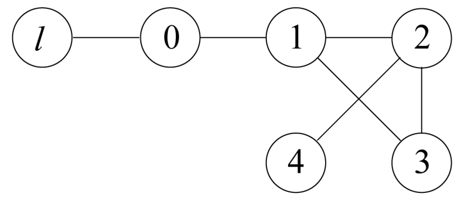
2.2. Algebraic Graph Theory

$G=(V_g,{\epsilon }_g,A_g)$ is an undirected graph in this paper, with $V_g=\left\{v_1,v_2,\dots ,v_n\right\}$ being the node-set, ${\epsilon }_g\subseteq V_g\times V_g$ being the edge set, and $A_g=\left[a_{ij}\right]$ being the adjacency matrix, of which all the elements are non-negative. The adjacency matrix $A_g$ depicts the effectiveness of communication from agent j to agent i, where $a_{ij}$ denotes the communication weight corresponding to the edge, and diagonal element $a_{ii}=0$, $a_{ij}>0$. As an undirected graph, the adjacency element $a_{ij}=a_{ji}$ must be guaranteed to be satisfied. If any pair of unique nodes can be connected by an undirected path, then the graph is connected. The Laplacian matrix $L_g=\left[l_{ij}\right]\subset R^{n\times n}$ is defined as follows

$$L_g=D_g-A_g$$

where $D_g=diag\left\{d_1,d_2,\dots ,d_n\right\}, d_i={\sum }_{j=1}^n{a}_{ij}$ and $i=1,2,\dots ,n$. Defining the leader adjacency weight matrix as $B_g=diag\left\{b_1,b_2,\dots ,b_n\right\}$, where $b_i>0$, indicates an exchange of information between agent i and the leader, otherwise, $b_i=0,i=1,2,\dots ,n$. It is presupposed that there is always at least one agent linked to the leader and $b_1+b_2+\cdots +b_n>0$.

Theorem 3

([43]). G must be irreducible for the graph to be linked.

Theorem 4

([43]). $\widetilde{L_g}=L_g+B_g=\left[\begin{array}{ccc}{l}_{11}+b_1& \cdots & l_{1n}\\ ⋮& \ddots & ⋮\\ l_{n1}& \cdots & l_{nn}+b_n\end{array}\right]$ are positive, where $B_g$ is the leader adjacency weight matrix if the Laplacian matrix $L_g$ of the undirected graph G is irreducible.

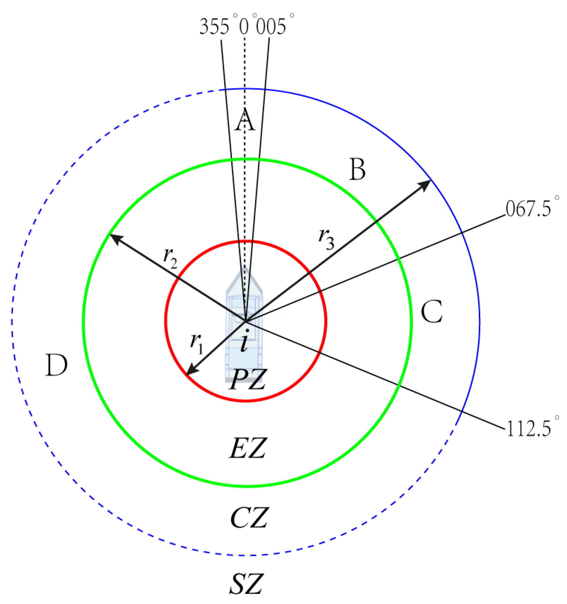
2.3. Improved Artificial Potential Field and Virtual Repulsion

The essential concept of the APF technique is that each agent is viewed as a high-potential field for the control objective of collision avoidance. Any agent that is close to the others will be repelled from their potential fields by the repulsive force. Specifically, the APF method has fewer design parameters and a significantly simpler controller architecture. Some results regard the agent as a particle, which makes collision avoidance issues impractical. In actuality, the domain of agents should be considered during an encounter situation. As illustrated in Figure 2, the domain of USV can be defined as three concentric circles with unequal radii.

As is shown in Figure 2, the repulsive force field is separated into the following four areas. The area outside the first circular area is defined as the Safe Zone, where $d_{ij}$ is greater than the detection distance $r_3$ of the potential field, there is no repulsive force in this area. The area inside the first circular area and outside the second circular is defined as the Negotiation Collision Avoidance Zone, where the distance $d_{ij}$ is larger than $r_2$ and less than or equal to $r_3$. If the incoming ship is in zones A, B, or C in the area, the i-th USV is a giving-way vessel or has the same avoidance responsibility, and the i-th USV should take collision avoidance actions to avoid the collision. If the incoming ship is in zone D, the i-th USV is a stand-on vessel. The area inside the second circular area and outside the third circular area is defined as the Emergency Collision Avoidance Zone, where the distance $d_{ij}$ is larger than $r_1$ and less than or equal to $r_2$. In the area where the distance between the other ship and the i-th USV is larger than and less than $r_2$, the i-th USV should perform emergency collision avoidance actions that can momentarily violate the COLREGs. The area within the third circular area is defined as the Prohibited Zone, which is shown by the red circular limit with radius $r_1$ in Figure 2. All other USVs are prohibited from entering this area.

Where $d_{ij}=x_i-x_j$ represents the relative position variable between the i-th USV and the incoming j-th USV, $∥d_{ij}∥$ represents the distance variable, and $r_3$ is the collision hazard detection distance, we conclude that the j-th USV is defined as a collision avoidance neighbor ${\mathsf{\Pi }}^c$ of the i-th USV. Once its collision avoidance neighbor ${\mathsf{\Pi }}^c$ holds $∥d_{ij}∥=∥x_i-x_j∥\le 2r_1$, it can be defined that the systems have been collided.

When the judgment condition ${355}^{\circ }\le T_r<{360}^{\circ }$ or $0^{\circ }\le T_r<{67.5}^{\circ }$, $r_2<d_{ij}\le r_3$ are met, the incoming j-th USV is in Zone A and Zone B. Meanwhile, when the judgment condition ${67.5}^{\circ }<T_r\le {112.5}^{\circ }$, $r_2<d_{ij}\le r_3$ are met, the incoming j-th USV is in Zone C. The i-th USV is a give-way ship. According to the COLREGs, it should turn right to give way. The repulsive force field is shown as follows [34]:

$${\phi }_{ij}(p,v)={\eta }_d{R}_j\left(e^{{\theta }_m-\theta }-1\right)\left(\frac{1}{d_{ij}-r_2}-\frac{1}{{\rho }_0}\right)$$

(14)

when the judgment condition $r_1<d_{ij}\le r_2$ is met, the i-th USV needs emergency collision avoidance. The repulsive force field is shown as follows:

$${\phi }_{ij}(p,v)={\eta }_d{R}_j\left[{\left(\frac{1}{d_{ij}-r_1}-\frac{1}{{\rho }_0}\right)}^2+{\left(∥v_{ot}∥cos\theta \right)}^2\right]$$

(15)

When $d_{ij}>r_2$ or the incoming j-th USV is in Zone D, the repulsion field is not defined, that is, the repulsion is zero.

Where p and v are the position and speed, $T_r$ denotes the relative position of the incoming j-th USV and the i-th USV, ${\eta }_d$ is the positive scaling factor for the USVs, $R_j$ is the radius of the puffing circle of the other ship, ${\rho }_0$ denotes the repulsive potential field’s influence radius of other ships, ${\theta }_m$ is the angle between the maximum relative position line, $\theta$ is the angle between $p_{ot}$, $v_{ot}$, $p_{ot}$ denotes the relative position line of the i-th USV and other ships, and $v_{ot}$ denotes the relative velocity.

The virtual repulsive force $f_{ij}^{ca}$ is defined as the negative gradient of the repulsive potential function ${\phi }_{ij}(p,v)$ as follows:

$$f_{ij}^{ca}=-{\nabla }_{(p,v)}{\phi }_{ij}(p,v)$$

(16)

where $-{\nabla }_{(p,v)}$ represents a negative gradient along p and v.

The total virtual repulsive force term of the whole systems is induced from (14)–(16) as follows:

$$\begin{array}{c}\hfill u_i^{ca}=-\frac{{\omega }_i}{{\vartheta }_i}\sum _{j\in {\mathsf{\Pi }}^c}{\nabla }_{(p,v)}{\phi }_{ij}(p,v)\end{array}$$

(17)

where ${\omega }_i$ denotes the positive gain parameter and ${\vartheta }_i$ is a positive constant.

3. Main Results

This section introduces a formation control protocol utilizing an extended state observer, aimed at guiding heterogeneous systems to follow a predefined trajectory in the XY plane, accounting for model uncertainties and external disturbances. Subsequently, a decentralized formation controller is developed to manage the height-tracking control of the UAV along the Z axis.

3.1. Controller Design Based on ESO

Rewrite (11) as

$$\left\{\begin{array}{c}{\dot{x}}_{i1}=x_{i2}\hfill \\ {\dot{x}}_{i2}=F_i+G_{xi}{u}_{xi}\hfill \end{array}\right.$$

(18)

where $F_i={\left[F_{Ti},F_{Li}\right]}^T=F_{xi}+{\Delta }_{xi}$, $F_{Ti}$ and $F_{Li}$ denote the transverse and longitudinal orientation of $F_i$ and $F_1$ denotes the sum of the nonlinear unknown term and the external disturbance encountered of the UAV. $F_2,F_3,F_4,F_5$ denote the sum of the nonlinear unknown term and the external disturbance encountered by different USVs, respectively.

For the purpose of approximating $F_i$, the design of an extended state observer has been formulated as follows

$$\left\{\begin{array}{c}{\dot{\widehat{x}}}_{i1}={\widehat{x}}_{i2}+\frac{{\alpha }_{i1}}{{\epsilon }_i}{k}_{xi}\hfill \\ {\dot{\widehat{x}}}_{i2}=G_{xi}{u}_{xi}+{\widehat{F}}_i+\frac{{\alpha }_{i2}}{{\epsilon }_i^2}{k}_{xi}\hfill \\ {\dot{\widehat{F}}}_i=\frac{{\alpha }_{i3}}{{\epsilon }_i^3}{k}_{xi}\hfill \end{array}\right.$$

(19)

where ${\widehat{x}}_{i1}, {\widehat{x}}_{i2}, {\widehat{F}}_i$ represent the observer state, ${\epsilon }_i>0$, ${\alpha }_{i1}\in \mathbb{R}, {\alpha }_{i2}\in \mathbb{R}, {\alpha }_{i3}\in \mathbb{R}$ are positive constants, $k_{xi}=x_{i1}-{\widehat{x}}_{i1}$. According to (19), we have

$$\left\{\begin{array}{c}{\dot{\tilde{x}}}_{i1}={\tilde{x}}_{i2}+\frac{{\alpha }_{i1}}{{\epsilon }_i}{k}_{xi}\hfill \\ {\dot{\tilde{x}}}_{i2}={\tilde{F}}_i+\frac{{\alpha }_{i2}}{{\epsilon }_i^2}{k}_{xi}\hfill \\ {\dot{\tilde{F}}}_i=\frac{{\alpha }_{i3}}{{\epsilon }_i^3}{k}_{xi}-{\dot{F}}_i\hfill \end{array}\right.$$

(20)

where ${\tilde{x}}_{i1}={\widehat{x}}_{i1}-x_{i1}$ is the ESO estimation error.

Define ${\eta }_i$ as

$${\eta }_i={\left[\begin{array}{ccc}{\eta }_{i1}\hfill & {\eta }_{i2}\hfill & {\eta }_{i3}\hfill \end{array}\right]}^T$$

where

$${\eta }_{i1}=\frac{x_{i1}-{\widehat{x}}_{i1}}{{\epsilon }_i^2},{\eta }_{i2}=\frac{x_{i2}-{\widehat{x}}_{i2}}{{\epsilon }_i},{\eta }_{i3}=F_i-{\widehat{F}}_i$$

The observation error equation of state can be written as

$$\begin{array}{c}\hfill {\epsilon }_i\dot{{\eta }_i}={\overline{A}}_i{\eta }_i+{\epsilon }_i{\overline{B}}_i{\dot{F}}_i\end{array}$$

(21)

where

$${\overline{A}}_i=\left[\begin{array}{ccc}-{\alpha }_{i1}\hfill & 1\hfill & 0\hfill \\ -{\alpha }_{i2}\hfill & 0\hfill & 1\hfill \\ -{\alpha }_{i3}\hfill & 0\hfill & 0\hfill \end{array}\right],{\overline{B}}_i=\left[\begin{array}{c}0\hfill \\ 0\hfill \\ 1\hfill \end{array}\right]$$

The error in position and velocity for heterogeneous systems within the XY plane is defined as follows

$$\begin{array}{c}{e}_i^{x_1}=\sum _{j\in \mathsf{\Pi }}{a}_{ij}\left(\left(x_{1i}-x_{1j}\right)-\left({\delta }_i-{\delta }_j\right)\right)\hfill \\ +b_i\left(x_{1i}-x_{1l}-{\delta }_i\right)\hfill \end{array}$$

(22)

$$e_i^{x_2}=\sum _{j\in \mathsf{\Pi }}{a}_{ij}\left(x_{2i}-x_{2j}\right)+b_i\left(x_{2i}-x_{2l}\right)$$

(23)

The formation control term is designed as follows

$$u_i^f=\frac{1}{{\vartheta }_i}\left[-{\widehat{F}}_i-k_i\left(e_i^{x_1}+e_i^{x_2}\right)\right]$$

(24)

Furthermore, the distributed formation controller with collision avoidance performance can be defined as follows

$$u_i=u_i^f+u_i^{ca}$$

(25)

Remark 1. 

In the formation controller (25), the distributed formation control term $u_i^f$ is used by tracking the time-varying velocity variable of the leader. The virtual repulsive force term $u_i^{ca}$ is used to achieve the collision avoidance objective among the agents. By designing the action functions (14) and (15) of the APF, they are non-conflicting items.

Using (17) and (24), distributed formation controller (25) can be given as

$$u_i=\frac{1}{{\vartheta }_i}\left[-{\widehat{F}}_i-k_i\left(e_i^{x_1}+e_i^{x_2}\right)\right]-\frac{{\omega }_i}{{\vartheta }_i}\sum _{j\in {\mathsf{\Pi }}^c}{\nabla }_{(p,v)}{\phi }_{ij}(p,v)$$

(26)

Take the derivative of (13) and substitute (11) and (12) into it. Define the derivatives of the error variables and write them in vector form as follows

$$\dot{\overline{Z}}=-\left[M\otimes I_m\right]\overline{Z}+\left[\begin{array}{c}{0}_{nm}\\ F_{xi}\end{array}\right]+\left[\begin{array}{c}{0}_{nm}\\ U\end{array}\right]+\left[\begin{array}{c}{0}_{nm}\\ {\Delta }_{xi}\end{array}\right]-\left[\begin{array}{c}{0}_{nm}\\ F_l\end{array}\right]$$

(27)

where $\dot{\overline{Z}}={\left[{\dot{\overline{x}}}_{11}^T,\dots ,{\dot{\overline{x}}}_{n1}^T,{\dot{\overline{x}}}_{12}^T,\dots ,{\dot{\overline{x}}}_{n2}^T\right]}^T$, $U=G_{xi}{u}_{xi}$, $M=\left[\begin{array}{cc}{0}_n& -I_n\\ 0_n& 0_n\end{array}\right]$, ⊗ denotes the Kronecker product.

3.2. Altitude Controller Design for UAV

The error system of altitude is defined as

$$e_{zp}=p_{az}-c_p$$

(28)

$$e_{zv}=v_{az}-c_v$$

(29)

where the desired position signal is $c_p$ and the desired velocity signal is $c_v$.

The adaptive laws and control input of formation tracking are constructed as

$$u_{az}={\widehat{H}}_{az}^{-1}\left(-\sigma e_{\zeta }-\frac{e_{\zeta }{\widehat{\kappa }}_{11}{\omega }_1^T{\omega }_1}{2{\varsigma }_1^2}-\frac{e_{\zeta }{\widehat{\kappa }}_{12}}{2{\varsigma }_2^2}+{\dot{c}}_v-k_{\zeta }{e}_{zv}\right)$$

(30)

$${\dot{\widehat{\kappa }}}_{11}=l_{11}\left(-k_{11}{\widehat{\kappa }}_{11}+\frac{e_{\zeta }^T{e}_{\zeta }{\omega }_1^T{\omega }_1}{2{\varsigma }_1^2}\right)$$

(31)

$${\dot{\widehat{\kappa }}}_{12}=l_{12}\left(-k_{12}{\widehat{\kappa }}_{12}+\frac{e_{\zeta }^T{e}_{\zeta }}{2{\varsigma }_2^2}\right)$$

(32)

$${\dot{\widehat{H}}}_{az}={Proj}_{\left[{\underline{H}}_{az},{\overline{H}}_{az}\right]}\left\{\mathcal{F}\right\}=\left\{\begin{array}{cc}0,\hfill & \mathrm{if}{\widehat{H}}_{az}={\overline{H}}_{az}\hfill \\ \hfill & \mathrm{and}\mathcal{F}\ge 0\hfill \\ \hfill & \mathrm{or}{\widehat{H}}_{az}={\underline{H}}_{az}\hfill \\ \hfill & \mathrm{and}\mathcal{F}\le 0\hfill \\ \mathcal{F},\hfill & \mathrm{otherwise}\hfill \end{array}\right.$$

(33)

where $\mathcal{F}=l_{13}\left(-k_{13}{\widehat{H}}_{az}+e_{\zeta }{u}_{az}\right), {\underline{H}}_{az}$, and ${\overline{H}}_{az}$ are the parameter $H_{az}$’s lower bound and upper bound of, respectively, where $\sigma ,k_{11}, k_{12}, k_{13}, k_{\zeta }, l_{11}, l_{12}, l_{13}, {\varsigma }_1, {\varsigma }_2$ denote positive parameters.

3.3. Stability Analysis

• Part A. Proof of the stability of the extended state observer

Consider the following Lyapunov function

$$V_0=\sum _{i=1}^{N+1}{V}_{0i}$$

(34)

where $V_{0i}$ is given as

$$V_{0i}={\epsilon }_i{{\eta }_i}^T{P}_i{\eta }_i$$

(35)

$$\begin{array}{cc}\hfill {\dot{V}}_{0i}& ={\epsilon }_i{\dot{{\eta }_i}}^T{P}_i{\eta }_i+{\epsilon }_i{\eta }_i^T{P}_i\dot{{\eta }_i}\hfill \\ & ={({\overline{A}}_i{\eta }_i+{\epsilon }_i{\overline{B}}_i{\dot{F}}_i)}^T{P}_i{\eta }_i+{{\eta }_i}^T{P}_i({\overline{A}}_i{\eta }_i+{\epsilon }_i{\overline{B}}_i{\dot{F}}_{ni})\hfill \\ & ={{\eta }_i}^T{\overline{A}}_i^T{P}_i{\eta }_i+{\epsilon }_i{\left({\overline{B}}_i{\dot{F}}_{ni}\right)}^{T}P{\eta }_i\hfill \\ & +{{\eta }_i}^T{P}_i{\overline{A}}_i{\eta }_i+\epsilon {{\eta }_i}^T{P}_i{\overline{B}}_i{\dot{F}}_{ni}\hfill \\ & ={{\eta }_i}^T\left({\overline{A}}_i^T{P}_i+P_i{\overline{A}}_i\right){\eta }_i+2{\epsilon }_i{{\eta }_i}^T{P}_i{\overline{B}}_i{\dot{F}}_{ni}\hfill \\ & ⩽-{{\eta }_i}^T{Q}_i{\eta }_i+2{\epsilon }_i\parallel P_i{\overline{B}}_i\parallel ·\parallel {\eta }_i\parallel ·|{\dot{F}}_i|\hfill \end{array}$$

(36)

and

$${\dot{V}}_{0i}⩽-{\lambda }_{min}\left(Q_i\right)\parallel {\eta }_i{\parallel }^2+2{\epsilon }_i|{\dot{F}}_i|\parallel P_i{\overline{B}}_i\parallel \parallel {\eta }_i\parallel$$

(37)

Therefore, the convergence condition of the observer satisfies

$$\begin{array}{c}\hfill \parallel {\eta }_i\parallel ⩽\frac{2{\epsilon }_i|{\dot{F}}_i|\parallel P{\overline{B}}_i\parallel }{{\lambda }_{min}\left(Q_i\right)}\end{array}$$

(38)

where $Q_i$ denotes any given symmetric positive definite matrix, ${\lambda }_{min}\left(Q_i\right)$ is the minimum eigenvalue of $Q_i$, and there is a three-by-three symmetric positive definite matrix $P_i$ that satisfies the following equation

$${\overline{A}}_i^T{P}_i+{P_i\overline{A}}_i+Q_i=0$$

(39)

Remark 2. 

Based on Assumptions 2 and 3, both the velocity and acceleration of the agent, as well as the external disturbances, are bounded. From $F_i=F_{xi}+{\Delta }_{xi}$, it is evident that $F_i$ encompasses the agent’s velocity and acceleration, as well as external disturbances. So, $|{\dot{F}}_i|$ is bounded.

• Part B. Proof of the stability of the system

Define the Lyapunov quadratic scalar function as follows

$$V_1=\frac{1}{2}{\overline{Z}}^T\left(P_g\otimes I_m\right)\overline{Z}$$

(40)

where $P=\left[\begin{array}{cc}2{\tilde{L}}_g& {\tilde{L}}_g\\ {\tilde{L}}_g& {\tilde{L}}_g\end{array}\right]$, ${\tilde{L}}_g=L_g+B_g$.

According to Theorem 4, the Lyapunov quadratic scalar function $V_1$ is a positive definite function.

Substitute (27) into $\dot{V_1}$ and expand the partial matrix as follows

$$\begin{array}{cc}\hfill \dot{V_1}=& {\overline{Z}}^T\left(P_g\otimes I_m\right)\dot{\overline{Z}}\hfill \\ \hfill =& -\frac{1}{2}{\overline{Z}}^T\left(\left(M^T{P}_g+P_{g}M\right)\otimes I_m\right)\overline{Z}+{\overline{Z}}^T\left(P_g\otimes I_m\right)\left[\begin{array}{c}{0}_{nm}\\ F_{xi}+U+{\Delta }_{xi}-F_l\end{array}\right]\hfill \\ \hfill =& -{\overline{Z}}^T\left(\left[\begin{array}{cc}{0}_n& -{\tilde{L}}_g\\ -{\tilde{L}}_g& -{\tilde{L}}_g\end{array}\right]\otimes I_m\right)\overline{Z}+\sum _{i=1}^n{\left(e_i^{x_1}+e_i^{x_2}\right)}^T\left(F_{xi}+G_{xi}{u}_{xi}+{\Delta }_{xi}-F_l\right)\hfill \end{array}$$

(41)

Substituting the distributed formation controller (24) into (41), we can obtain

$$\begin{array}{cc}\hfill \dot{V_1}=& -{\overline{Z}}^T\left(\left[\begin{array}{cc}{0}_n& -{\tilde{L}}_g\\ -{\tilde{L}}_g& -{\tilde{L}}_g\end{array}\right]\otimes I_m\right)\overline{Z}\hfill \\ & +\sum _{i=1}^n{\left(e_i^{x_1}+e_i^{x_2}\right)}^T{F}_{xi}-\sum _{i=1}^n{\left(e_i^{x_1}+e_i^{x_2}\right)}^T{F}_l+\sum _{i=1}^n{\left(e_i^{x_1}+e_i^{x_2}\right)}^T\hfill \\ & \times \left(-{\widehat{F}}_i-k_i\left(e_i^{x_1}+e_i^{x_2}\right)-{\omega }_i\sum _{j\in {\mathsf{\Pi }}^c}{\nabla }_{(p,v)}{\phi }_{ij}(p,v)\right)\hfill \\ & =-{\overline{Z}}^T\left(\left[\begin{array}{cc}{0}_n\hfill & -{\tilde{L}}_g\hfill \\ -{\tilde{L}}_g\hfill & -{\tilde{L}}_g\hfill \end{array}\right]\otimes I_m\right)\overline{Z}-\sum _{i=1}^n{\left(e_i^{x_1}+e_i^{x_2}\right)}^T{F}_l\hfill \\ & -\sum _{i=1}^n{k}_i{∥\left(e_i^{x_1}+e_i^{x_2}\right)∥}^2-\sum _{i=1}^n{\left(e_i^{x_1}+e_i^{x_2}\right)}^T\times {\omega }_i\sum _{j\in {\mathsf{\Pi }}^c}{\nabla }_{(p,v)}{\phi }_{ij}(p,v)\hfill \end{array}$$

(42)

In the case of an undirected graph, the Laplacian matrix exhibits symmetry, and the virtual repulsive force term $u_i^{ca}$ becomes negligible once collision avoidance is achieved through the repulsive potential function ${\phi }_{ij}(p,v)$.

Therefore, the aforementioned term $V^{\prime }=-{\sum }_{i=1}^n{\left(e_i^{x_1}+e_i^{x_2}\right)}^T{\omega }_i{\sum }_{j\in {\mathsf{\Pi }}^c}{\nabla }_{(p,v)}{\phi }_{ij}(p,v)=0$, based on Assumption 1 and Young’s inequality as follows

$$-{\left(e_i^{x_1}+e_i^{x_2}\right)}^T{F}_l\le {\xi }_i{∥e_i^{x_1}+e_i^{x_2}∥}^2+\frac{{\alpha }_l^2}{4{\xi }_i}$$

where ${\xi }_i$ is a positive constant.

And then the results (42) can be derived as follows

$$\begin{array}{cc}\hfill \dot{V_1}\le & -{\overline{Z}}^T\left(\left[\begin{array}{cc}{0}_n& -{\tilde{L}}_g\\ -{\tilde{L}}_g& -{\tilde{L}}_g\end{array}\right]\otimes I_m\right)\overline{Z}+\sum _{i=1}^n{\xi }_i{∥e_i^{x_1}+e_i^{x_2}∥}^2+\sum _{i=1}^n\frac{{\alpha }_l}{4{\xi }_i}-\sum _{i=1}^n{k}_i{∥\left(e_i^{x_1}+e_i^{x_2}\right)∥}^2\hfill \\ \hfill =& -{\overline{Z}}^T\left(\left[\begin{array}{cc}{0}_n& -{\tilde{L}}_g\\ -{\tilde{L}}_g& -{\tilde{L}}_g\end{array}\right]\otimes I_m\right)\overline{Z}+\sum _{i=1}^n\left({\xi }_i-k_i\right){∥e_i^{x_1}+e_i^{x_2}∥}^2+\sum _{i=1}^n\frac{{\alpha }_l^2}{4{\xi }_i}\hfill \end{array}$$

(43)

Let ${\rho }_i$ satisfy the limit of ${\rho }_i\le k_i-{\xi }_i$ and ${\rho }_i>0$, the inequality is transformed into

$$\begin{array}{cc}\hfill \dot{V_1}& \le -{\overline{Z}}^T\left(\left[\begin{array}{cc}{0}_n& -{\tilde{L}}_g\\ -{\tilde{L}}_g& -{\tilde{L}}_g\end{array}\right]\otimes I_m\right)\overline{Z}-\sum _{i=1}^n{\rho }_i{∥e_i^{x_1}+e_i^{x_2}∥}^2+\sum _{i=1}^n\frac{{\alpha }_l^2}{4{\xi }_i}\hfill \\ & =-{\overline{Z}}^T\left(\left({\rho }_i\left[\begin{array}{cc}{\tilde{L}}_g^2& {\tilde{L}}_g^2\\ {\tilde{L}}_g^2& {\tilde{L}}_g^2\end{array}\right]-\left[\begin{array}{cc}{0}_n& {\tilde{L}}_g\\ {\tilde{L}}_g& {\tilde{L}}_g\end{array}\right]\right)\otimes I_m\right)\overline{Z}+\sum _{i=1}^n\frac{{\alpha }_l^2}{4{\xi }_i}\hfill \\ & =-{\overline{Z}}^T\left(\left[\begin{array}{cc}{\rho }_i{\tilde{L}}_g^2& {\rho }_i{\tilde{L}}_g^2-{\tilde{L}}_g\\ {\rho }_i{\tilde{L}}_g^2-{\tilde{L}}_g& {\rho }_i{\tilde{L}}_g^2-{\tilde{L}}_g\end{array}\right]\otimes I_m\right)\overline{Z}+\sum _{i=1}^n\frac{{\alpha }_l^2}{4{\xi }_i}\hfill \end{array}$$

(44)

According to the Lemma of linear matrix inequality in [41], ${\rho }_i{\tilde{L}}_g^2-\left({\rho }_i{\tilde{L}}_g^2-{\tilde{L}}_g\right)={\tilde{L}}_g^2>0,{\rho }_i{\tilde{L}}_g^2-{\tilde{L}}_g>0$, so the matrix $\left[\begin{array}{cc}{\rho }_i{\tilde{L}}_g^2& {\rho }_i{\tilde{L}}_g^2-{\tilde{L}}_g\\ {\rho }_i{\tilde{L}}_g^2-{\tilde{L}}_g& {\rho }_i{\tilde{L}}_g^2-{\tilde{L}}_g\end{array}\right]>0$. Therefore, the inequality (44) can be rewritten as follows

$$\begin{array}{cc}\hfill \dot{V_1}\le & -{\overline{Z}}^T\left(\left({\rho }_i\left[\begin{array}{cc}{\tilde{L}}_g^2& {\tilde{L}}_g^2\\ {\tilde{L}}_g^2& {\tilde{L}}_g^2\end{array}\right]-\left[\begin{array}{cc}{0}_n& {\tilde{L}}_g\\ {\tilde{L}}_g& {\tilde{L}}_g\end{array}\right]\right)\otimes I_m\right)\overline{Z}+\sum _{i=1}^n\frac{{\alpha }_l^2}{4{\xi }_i}\hfill \\ \hfill =& -{\overline{Z}}^T\left(\left({\rho }_i\mathsf{\Theta }-\mathsf{\Xi }\right)\otimes I_m\right)\overline{Z}+\Delta \hfill \end{array}$$

(45)

where

$$\mathsf{\Theta }=\left[\begin{array}{cc}{\tilde{L}}_g^2& {\tilde{L}}_g^2\\ {\tilde{L}}_g^2& {\tilde{L}}_g^2\end{array}\right], \mathsf{\Xi }=\left[\begin{array}{cc}{0}_n& {\tilde{L}}_g\\ {\tilde{L}}_g& {\tilde{L}}_g\end{array}\right], \Delta =\sum _{i=1}^n\frac{{\alpha }_l^2}{4{\xi }_i}.$$

Set ${\rho }_i>\frac{1}{{\lambda }_{min}^{\mathsf{\Theta }}}\left({\lambda }_{max}^{\mathsf{\Xi }}+\frac{\Im }{2}{\lambda }_{max}^P\right)$, where ${\lambda }_{min}^{\mathsf{\Theta }},{\lambda }_{max}^{\mathsf{\Xi }},{\lambda }_{max}^P$ denote the smallest eigenvalue of the matrix $\mathsf{\Theta }$, the largest eigenvalue of the matrix $\mathsf{\Xi }$, and the largest eigenvalue of the matrix P, respectively, and $\Im =min\left\{{\sigma }_1{\mathrm{Y}}_1,\dots ,{\sigma }_n{\mathrm{Y}}_n\right\}$.

Then, we can obtain

$$\begin{array}{cc}\hfill \dot{V_1}& \le -\Im {\overline{Z}}^T\left(P\otimes I_m\right)\overline{Z}+\Delta \hfill \\ & =-\Im V_1+\Delta \hfill \end{array}$$

(46)

In accordance with Theorem 1, the subsequent inequality can be presented in the following manner

$$V_1\left(t\right)\le V_1\left(0\right)e^{-\Im t}+\frac{\Delta }{\Im }\left(1-e^{-\Im t}\right)$$

(47)

Consequently, by choosing suitable parameters as indicated in [44], one can achieve the performance of adaptive leader-following formation.

• Part C. Proof of collision avoidance

The collision avoidance performance is analyzed only for the i-th $(i\in \mathsf{\Pi })$ USV and its collision avoidance neighbor the j-th $(j\in {\mathsf{\Pi }}^c)$ USV, and the others can be analyzed by the same way in [42].

Define the energy function holds quadratic form as follows

$$S\left(t\right)=\frac{1}{2}{v}_i^T\left(t\right)v_i\left(t\right)+\frac{1}{2}{d}_{ik}^T\left(t\right)d_{ik}\left(t\right)$$

(48)

Taking the time derivative of (48), we can get

$$\begin{array}{cc}\hfill \dot{S}\left(t\right)=& {\omega }_i{v}_i^T\left(t\right){\nabla }_{(p,v)}{\phi }_{ij}(p,v)+d_{ik}^T\left(t\right)\left(v_i\left(t\right)-v_k\left(t\right)\right)-v_i^T\left(t\right){\widehat{F}}_i-k_i{v}_i^T\left(t\right)\left(e_i^{x_1}\left(t\right)+e_i^{x_2}\left(t\right)\right)\hfill \end{array}$$

(49)

where $d_{ik}\left(t\right)$ is the relative position variable.

Because of the designing of the repulsive potential function ${\phi }_{ij}(p,v)$, ${\phi }_i\left(d_{ik}\left(t\right)\right)$ will approach infinity by designing the parameter ${\overline{\omega }}_i>0$ if the i-th USV is closing to the j-th USV. Therefore, if the i-th USV and the j-th USV are close to each other, and design the appropriate parameter, the inequality can be met in the following manner:

$$\begin{array}{c}{v}_i^T\left(t\right){\nabla }_{(p,v)}{\phi }_{ij}(p,v)>\frac{1}{2}{d}_{ik}^T\left(t\right)d_{ik}\left(t\right)+\frac{1}{2}{v}_i^T\left(t\right)v_i\left(t\right)\hfill \\ -\frac{1}{{\omega }_i}{d}_{ik}^T\left(t\right)\left(v_i\left(t\right)-v_k\left(t\right)\right)+\frac{1}{{\omega }_i}{v}_i^T\left(t\right){\widehat{F}}_i\hfill \\ +\frac{k_i}{{\omega }_i}{v}_i^T\left(t\right)\left(e_i^{x_1}\left(t\right)+e_i^{x_2}\left(t\right)\right)\hfill \end{array}$$

(50)

Substituting the aforementioned inequality (50) into (49), the subsequent inequality can be derived

$$\dot{S}\left(t\right)>{\omega }_{i}S\left(t\right)$$

Based on the principles outlined in Theorem 2, the subsequent inequality can be derived

$$d_{ik}^T\left(t\right)d_{ik}\left(t\right)>2e^{{\omega }_i\left(t-t_0\right)}S\left(t\right)-v_i^T\left(t\right)v_i\left(t\right)$$

Since the previously indicated term $v_i^T\left(t\right)v_i\left(t\right)$ is continuous and bounded at this dwell time. By designing the gain parameter ${\omega }_i>0$ large enough, we get can the inequality $2e^{{\omega }_i\left(t-t_0\right)}S\left(t\right)-v_i^T\left(t\right)v_i\left(t\right)>{\left(2r_1\right)}^2$ and the result can be obtained as $∥d_{ik}\left(t\right)∥>2r_1$. As a result, the collision avoidance performance can be guaranteed by the proposed formation control with collision avoidance strategy.

• Part D. Proof of the decentralized formation controller

If the feasibility condition $c_v-{\dot{c}}_p=0$ is satisfied, it then allows the time derivative of Equations (28) and (29) to be expressed as follows

$${\dot{e}}_{zp}=e_{zv}$$

(51)

$${\dot{e}}_{zv}=F_{az}+G_{az}{u}_{az}+{\Delta }_{az}-{\dot{c}}_v.$$

(52)

where $e_{zv}$ may be regarded as the virtual control input in the system (51). The stability of the system (51) can be assured by constructing the virtual control input $\zeta =-k_{\zeta }{e}_{zp}$.

A positive Lyapunov function is considered as

$$V_{zp}=\frac{1}{2}{e}_{zp}^T{e}_{zp}$$

(53)

A new error is defined as

$$e_{\zeta }=e_{zv}-\zeta$$

(54)

By computing the time derivative of Equation (53) and incorporating the control input from Equation (30) into this calculation, one can obtain

$${\dot{e}}_{\zeta }=-\sigma e_{\zeta }+F_{az}+{\Delta }_{az}+{\tilde{H}}_{az}{u}_{az}-\frac{e_{\zeta }{\widehat{\kappa }}_{11}{\omega }_1^T{\omega }_1}{2{\varsigma }_1^2}-\frac{e_{\zeta }{\widehat{\kappa }}_{12}}{2{\varsigma }_2^2}.$$

(55)

$V_z$ is given as

$$V_z=\frac{1}{2}{e}_{zp}^T{e}_{zp}+\frac{1}{2}{e}_{\zeta }^T{e}_{\zeta }+\frac{{\tilde{\kappa }}_{11}^2}{2l_{11}}+\frac{{\tilde{\kappa }}_{12}^2}{2l_{12}}+\frac{Tr\left({\tilde{H}}_{az}^T{\tilde{H}}_{az}\right)}{2l_{13}}$$

(56)

with ${\tilde{\kappa }}_{11}={\kappa }_{11}-{\widehat{\kappa }}_{11}, {\tilde{\kappa }}_{12}={\kappa }_{12}-{\widehat{\kappa }}_{12}$ and ${\tilde{H}}_{az}=H_{az}-{\widehat{H}}_{az}$.

$$\begin{array}{cc}\hfill {\dot{V}}_z\le & -k_{\zeta }{e}_{zp}^T{e}_{zp}-\sigma e_{\zeta }^T{e}_{\zeta }+e_{\zeta }^T{F}_{az}+e_{\zeta }^T{\Delta }_{az}\hfill \\ & +e_{\zeta }^T{\tilde{H}}_{az}{u}_{az}-\frac{e_{\zeta }^T{e}_{\zeta }{\widehat{\kappa }}_{11}{\omega }_1^T{\omega }_1}{2{\varsigma }_1^2}-\frac{e_{\zeta }^T{e}_{\zeta }{\widehat{\kappa }}_{12}}{2{\varsigma }_2^2}+\frac{{\tilde{\kappa }}_{11}{\dot{\tilde{\kappa }}}_{11}}{l_{11}}+\frac{{\tilde{\kappa }}_{12}{\dot{\tilde{\kappa }}}_{12}}{l_{12}}+\frac{Tr\left({\tilde{H}}_{az}^T{\dot{\tilde{H}}}_{az}\right)}{l_{13}}\hfill \end{array}$$

(57)

Given that $F_{az}$ is an undefined function, as per the universal approximation theorem cited in [45], for any arbitrarily small constant ${ϵ}_1$, there exists a fuzzy logic system ${\theta }_1^{*T}{\omega }_1$ that can be represented as $F_{az}={\theta }_1^{*T}{\omega }_1+{ϵ}_1$. In this context, ${\theta }_1^{*T}$ represents the optimal weight, ${\omega }_1$ is the fuzzy basis vector, ${ϵ}_1$ denotes the fuzzy system’s approximation error, and it is established that $\left|{ϵ}_1\right|\le {\overline{ϵ}}_1$.

Regarding Young’s inequality, it can be deduced that

$$e_{\zeta }^T{\theta }_1^{*T}{\omega }_1\le \frac{e_{\zeta }^T{e}_{\zeta }{\kappa }_{11}{\omega }_1^T{\omega }_1}{2{\varsigma }_1^2}+\frac{{\varsigma }_1^2}{2}$$

(58)

$$e_{\zeta }^T\left({ϵ}_1+{\Delta }_{az}\right)\le \frac{e_{\zeta }^T{e}_{\zeta }{\kappa }_{12}}{2{\varsigma }_2^2}+\frac{{\varsigma }_2^2}{2}$$

(59)

where ${\kappa }_{11}={\theta }_1^{*T}{\theta }_1^{*}$ and ${\kappa }_{12}={\left({\overline{ϵ}}_1+{\overline{\Delta }}_{az}\right)}^T\left({\overline{ϵ}}_1+{\overline{\Delta }}_{az}\right)$.

Substituting (58) and (59) into (57), we can obtain

$$\begin{array}{cc}\hfill {\dot{V}}_{iz}\le & -k_{\zeta }{e}_{zp}^T{e}_{zp}-\sigma e_{\zeta }^T{e}_{\zeta }+\frac{e_{\zeta }^T{e}_{\zeta }{\kappa }_{11}{\omega }_1^T{\omega }_1}{2{\varsigma }_1^2}+\frac{e_{\zeta }^T{e}_{\zeta }{\kappa }_{12}}{2{\varsigma }_2^2}\hfill \\ & -\frac{e_{\zeta }^T{e}_{\zeta }{\widehat{\kappa }}_{11}{\omega }_1^T{\omega }_1}{2{\varsigma }_1^2}-\frac{e_{\zeta }^T{e}_{\zeta }{\widehat{\kappa }}_{12}}{2{\varsigma }_2^2}-{\tilde{\kappa }}_{12}\left(-k_{12}{\widehat{\kappa }}_{12}+\frac{e_{\zeta }^T{e}_{\zeta }}{2{\varsigma }_2^2}\right)\hfill \\ & -{\tilde{\kappa }}_{11}\left(-k_{11}{\widehat{\kappa }}_{11}+\frac{e_{\zeta }^T{e}_{\zeta }{\omega }_1^T{\omega }_1}{2{\varsigma }_1^2}\right)+e_{\zeta }^T{\tilde{H}}_{az}{u}_{az}\hfill \\ & -Tr\left({\tilde{H}}_{az}^T\left(-k_{13}{\widehat{H}}_{az}+e_{\zeta }{u}_{az}\right)\right)+\frac{{\varsigma }_1^2}{2}+\frac{{\varsigma }_2^2}{2}\hfill \\ \hfill \le & -k_{\zeta }{e}_{zp}^T{e}_{zp}-\sigma e_{\zeta }^T{e}_{\zeta }-\frac{k_{11}}{2}{\tilde{\kappa }}_{11}^2-\frac{k_{12}}{2}{\tilde{\kappa }}_{12}^2-\frac{k_{13}}{2}{∥{\tilde{H}}_{az}∥}_F^2\hfill \\ & +\frac{k_{11}}{2}{\kappa }_{11}^2+\frac{k_{12}}{2}{\kappa }_{12}^2+\frac{k_{13}}{2}{∥H_{az}∥}_F^2+\frac{{\varsigma }_1^2}{2}+\frac{{\varsigma }_2^2}{2}\hfill \\ \hfill \le & -{\vartheta }_z{V}_z+v_z\hfill \end{array}$$

(60)

where ${\theta }_z=min\left\{2k_{\zeta },2\sigma ,l_{11}{k}_{11},l_{12}{k}_{12},l_{13}{k}_{13}\right\}>0$, $v_z=\frac{k_{11}}{2}{\kappa }_{11}^2+\frac{k_{12}}{2}{\kappa }_{22}^2+\frac{k_{13}}{2}{∥H_{az}∥}_F^2+\frac{{\varsigma }_1^2}{2}+\frac{{\varsigma }_2^2}{2}$.

Based on Equation (60), ${\dot{V}}_z$ is derived as follows

$${\dot{V}}_z\le -{\vartheta }_z{V}_z+v_z$$

(61)

According to the boundedness theorem, the closed-loop system solution is uniformly eventually bounded. Using $e_{zp}$ and $e_{\zeta }$, it is possible to deduce that the UAV’s velocity error and altitude tracking error are uniformly eventually bounded.

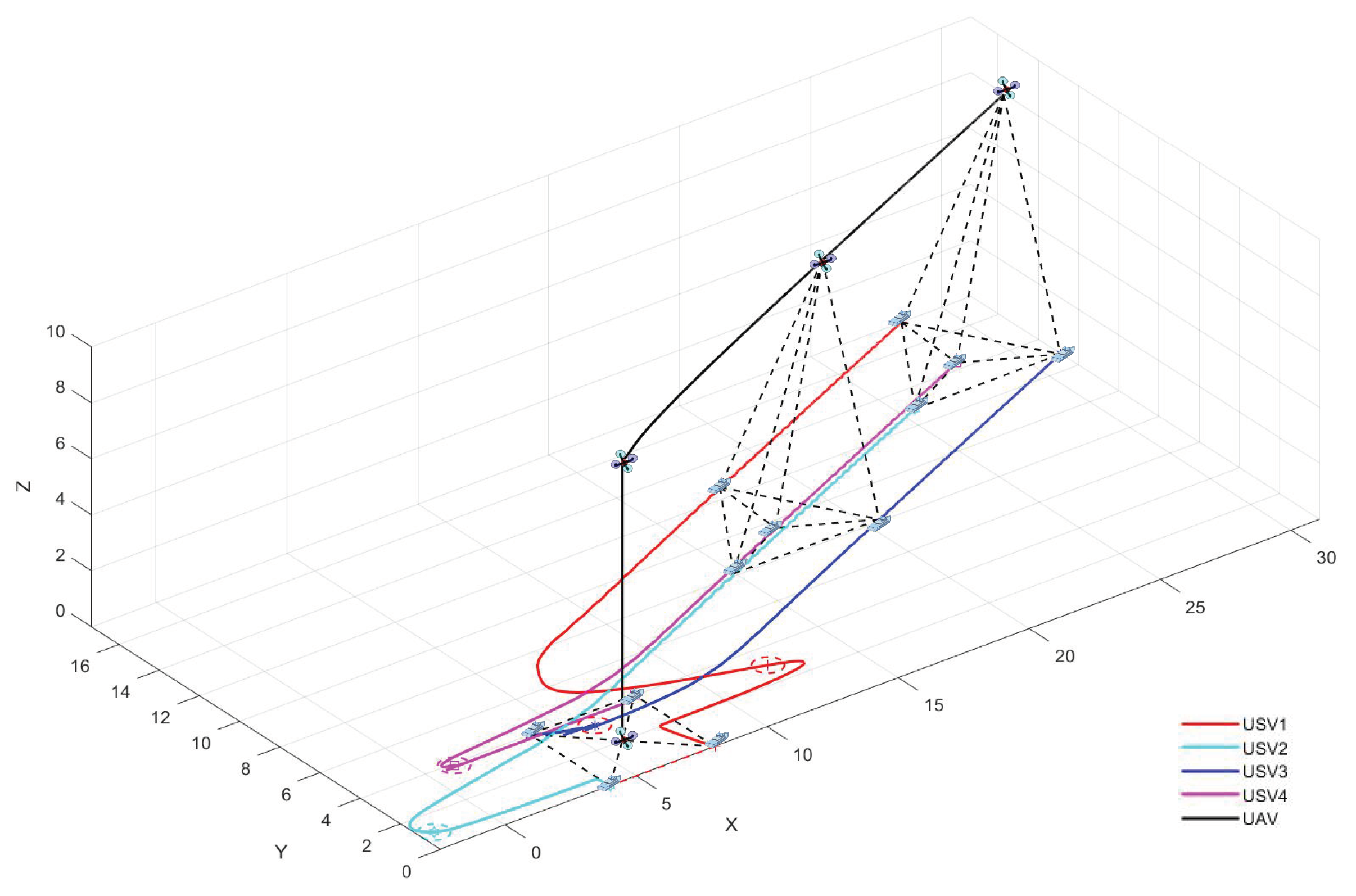
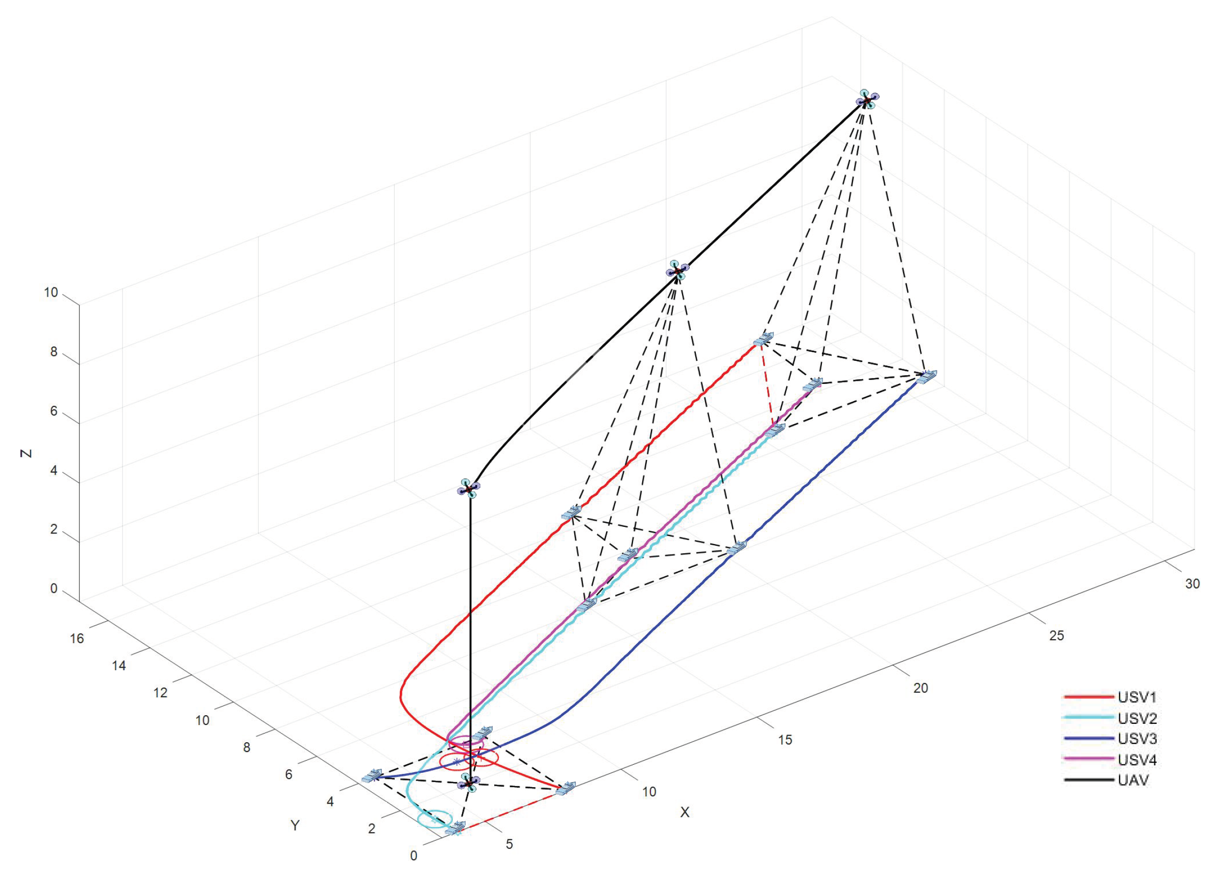
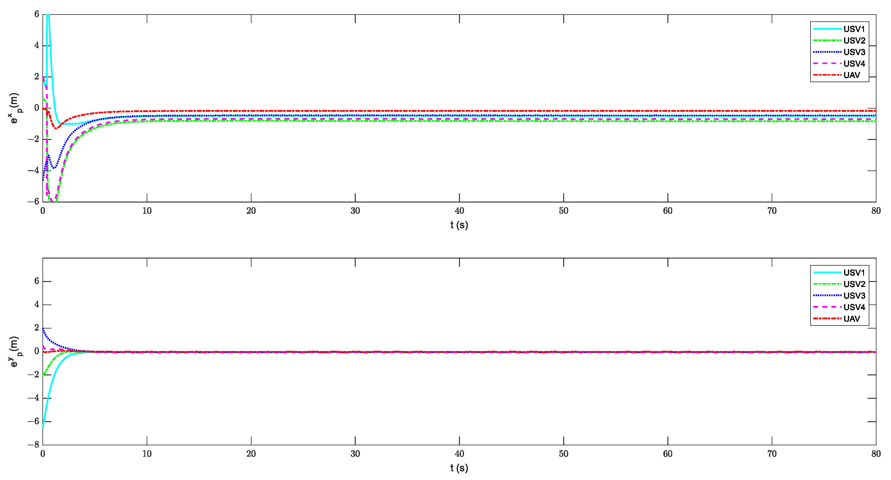
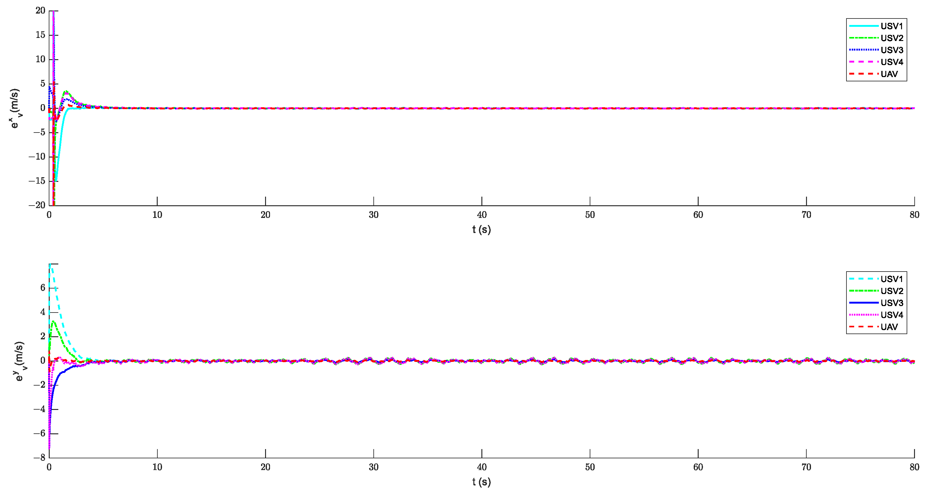
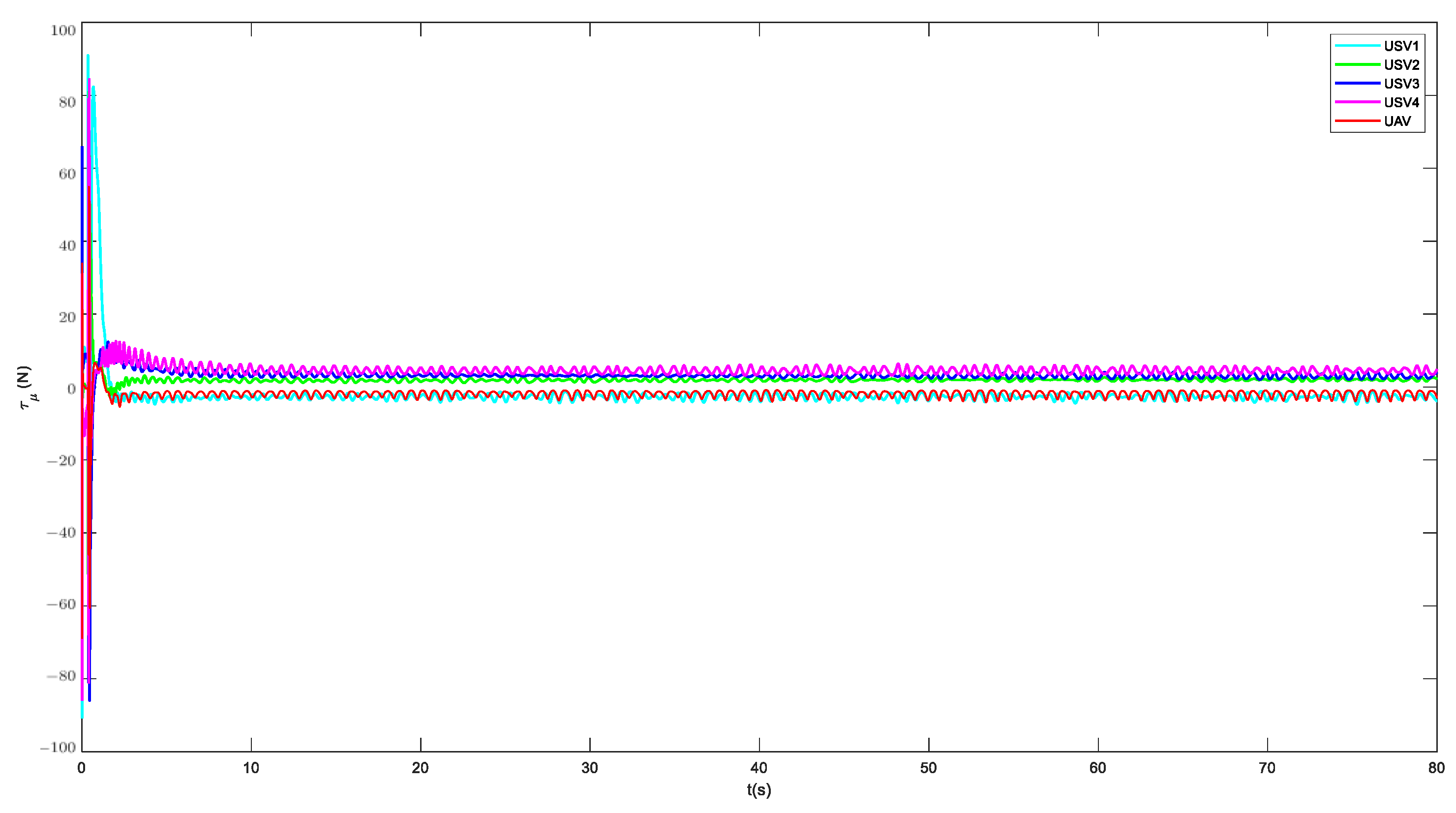
4. Simulation Result

In this section, a simulation analysis for the heterogeneous systems with collision avoidance performance under parameter uncertainty and external disturbance is provided to illustrate the effect of the proposed approach. One UAV and four USVs make up the heterogeneous system. The simulation experiments described in this section were executed on the MATLAB R2020a simulation platform.

The communication topology is defined in Figure 3, where agent l represents the virtual leader, agent 0 represents the UAV, and agents 1–4 represent the four USVs. If $B_g=diag\{0,0,0,0,1\}$ is the adjacency weight matrix between agents and the virtual leader, then the adjacency matrix $A_g$ and the Laplacian matrix $L_g$ are as follows:

$$A_g=\left[\begin{array}{ccccc}0\hfill & 1\hfill & 1\hfill & 0\hfill & 1\hfill \\ 1\hfill & 0\hfill & 1\hfill & 1\hfill & 0\hfill \\ 1\hfill & 1\hfill & 0\hfill & 0\hfill & 0\hfill \\ 0\hfill & 1\hfill & 0\hfill & 0\hfill & 0\hfill \\ 1\hfill & 0\hfill & 0\hfill & 0\hfill & 0\hfill \end{array}\right]\hspace{1em}{L}_g=\left[\begin{array}{ccccc}3& -1& -1& 0& -1\\ -1& 3& -1& -1& 0\\ -1& -1& 2& 0& 0\\ 0& -1& 0& 1& 0\\ -1& 0& 0& 0& 1\end{array}\right]$$

The system parameters of a UAV and USVs are given in

Table 1. The model parameters of UAV.

Parameter	Value	Unit
$m_a$	2	kg
$g_a$	9.8	$\mathrm{m}·{\mathrm{s}}^{-2}$
$J_{ax},J_{ay},J_{az}$	1.5	$\mathrm{N}·{\mathrm{s}}^2·{\mathrm{rad}}^{-1}$
$d_{ax},d_{ay},d_{az}$	0.012	$\mathrm{N}·{\mathrm{s}}^2·{\mathrm{rad}}^{-1}$

and

Table 2. The model parameters of USV.

Parameter	Value	Unit
$m_{\mu bi}$	25.8	kg
$m_{vbi}$	33.8	kg
$m_{rbi}$	2.76	kg
$d_{\mu bi}$	0.725	kg $·{\mathrm{s}}^{-1}$
$d_{vbi}$	0.89	kg $·{\mathrm{s}}^{-1}$
$d_{rbi}$	$-1.9$	kg $·{\mathrm{m}}^{-2}·{\mathrm{s}}^{-1}$
$d_{\mu bi1}$	$-1.33$	kg $·{\mathrm{s}}^{-1}$
$d_{vbi1}$	$-36.47$	kg $·{\mathrm{s}}^{-1}$
$d_{rbi1}$	$-0.75$	kg $·{\mathrm{m}}^{-2}·{\mathrm{s}}^{-1}$

, respectively. APF design parameters $r_{in}=0.5$, $r_{\mathrm{out}}=2$, ${\overline{\omega }}_i=0.3$, ${\omega }_i=1$, where $i=1,\dots ,4$. The external disturbances are given as ${\Delta }_{axy}=[0.2cos\left(0.5t\right)$, ${0.8cos\left(t\right)]}^T$, ${\Delta }_{az}=0.3cos\left(0.2t\right)$, $w_{bixy}={[1.1cos\left(0.5t\right),-0.2sin\left(2t\right)]}^T$. The total duration of the simulation runs $T_z=80 \mathrm{s}$ and the sampling time $T_s=0.6 \mathrm{s}$.

The initial position state vector of the UAV and USVs are defined as $x_0\left(0\right)={[6,2,10]}^T$, $x_1\left(0\right)={[8,0,0]}^T, x_2\left(0\right)={[4,0,0]}^T$, $x_3\left(0\right)={[4,4,0]}^T, x_4\left(0\right)={[8,4,0]}^T, {\delta }_0={[0,0]}^T, {\delta }_1={[0,3\aleph ]}^T, {\delta }_2={[-\sqrt{3}\aleph ,0]}^T, {\delta }_3={[\sqrt{3}\aleph ,0]}^T, {\delta }_4={[0,\aleph ]}^T, \aleph =\frac{3}{2}$.

The simulation results by using the proposed control method for heterogeneous systems with collision avoidance strategy are shown in Figure 4, Figure 5, Figure 6, Figure 7, Figure 8, Figure 9, Figure 10 and Figure 11. The trajectories of the four USVs and the UAV in the 3D environment are depicted in Figure 4. The black line represents the UAV’s trajectory, while the other color lines represent the trajectories of the four USVs. From the given starting point, the USVs maintain a safe distance and establish a designated configuration between each other. Figure 5 shows the trajectories of heterogeneous systems without collision avoidance. At the sampling time $T_s=0.6 \mathrm{s}$, Figure 5 shows that three USVs have been collided. Simulation trajectory plots demonstrate the importance of collision avoidance for heterogeneous systems.

Figure 6 and Figure 7 represent the position tracking errors and velocity errors in x-label and y-label, respectively. Under the influence of external disturbances and parameter uncertainties, the formation trajectory tracking errors are capable of converging to a minimal residual set. Figure 8 and Figure 9 depict the surge force and yaw torque. The outcomes of the simulations indicate that the USVs are able to continue tracking the virtual leader even after activating the improved APF for collision avoidance.

Figure 10 and Figure 11 further display the distances between USVs without and with considering the collision avoidance. Figure 10 shows that the USVs have collided, because of the distance ${∥d_{ij}∥}_{min}<2r_1=1$. Figure 11 shows that the distances of USVs can always maintain ${∥d_{ij}∥}_{min}>2r_1=1$ at any time. The simulation diagrams further confirm that the proposed formation control with collision avoidance strategy has an excellent performance. The performance of ESO in estimating $F_i$ is depicted in Figure 12, which clearly demonstrates the effectiveness of the proposed solution for the accurate compensation of uncertainties and external disturbances within heterogeneous systems.

5. Conclusions

In this paper, the cooperative formation trajectory tracking problem for heterogeneous systems with collision avoidance performance under parameter uncertainty and external disturbance is investigated. Under the unified dynamic model of a UAV and USVs in the XY plane, a formation control protocol based on ESO is proposed. The collision avoidance control approach for USV formation is then constructed using APF theory. Furthermore, the APF approach is improved by rebuilding the repulsive potential field to bring the unmanned ship’s collision avoidance behavior more in compliance with COLREGs. According to the Lyapunov stability theory, the time-varying formation errors and tracking errors are uniformly ultimately limited. Simulation results verify the effectiveness of the proposed scheme.

This paper focuses solely on heterogeneous formation and collision avoidance between a single UAV and multiple USVs. Going forward, cooperative collision avoidance involving multiple UAVs and USVs within intricate environments deserves further study. In discussions of formation control issues for multi-agent or multi-vehicle systems, it is common to assume that the controlled entities operate within an ideal network communication environment. However, in practical scenarios, such as with USVs, the communication environment is often fraught with issues like noise, time delays, and packet loss. Consequently, the problem of cooperative collision avoidance control for swarm systems under adverse communication conditions also merits thorough investigation.

References

1. Yan, X.; Jiang, D.; Miao, R.; Li, Y. Formation control and obstacle avoidance algorithm of a multi-USV system based on virtual structure and artificial potential field. J. Mar. Sci. Eng. 2021, 9, 161. [Google Scholar] [CrossRef]
2. Shan, Q.; Wang, X.; Li, T.; Chen, C.P. Finite-time control for USV path tracking under input saturation with random disturbances. Appl. Ocean Res. 2023, 138, 103628. [Google Scholar] [CrossRef]
3. Guerrero-Ibañez, J.; Contreras-Castillo, J.; Zeadally, S. Deep learning support for intelligent transportation systems. Trans. Emerg. Telecommun. Technol. 2021, 32, e4169. [Google Scholar] [CrossRef]
4. Li, X.; Tan, J.; Liu, A.; Vijayakumar, P.; Kumar, N.; Alazab, M. A Novel UAV-Enabled Data Collection Scheme for Intelligent Transportation System Through UAV Speed Control. IEEE Trans. Intell. Transp. Syst. 2021, 22, 2100–2110. [Google Scholar] [CrossRef]
5. Menouar, H.; Guvenc, I.; Akkaya, K.; Uluagac, A.S.; Kadri, A.; Tuncer, A. UAV-Enabled Intelligent Transportation Systems for the Smart City: Applications and Challenges. IEEE Commun. Mag. 2017, 55, 22–28. [Google Scholar] [CrossRef]
6. Sun, Y.; Zhang, D.; Wang, Y.; Zong, Z.; Wu, Z. Model Experimental Study on a T-Foil Control Method with Anti-Vertical Motion Optimization of the Mono Hull. J. Mar. Sci. Eng. 2023, 11, 1551. [Google Scholar] [CrossRef]
7. Ke, C.; Chen, H. Cooperative path planning for air–sea heterogeneous unmanned vehicles using search-and-tracking mission. Ocean Eng. 2022, 262, 112020. [Google Scholar] [CrossRef]
8. Ren, Y.; Zhang, L.; Ying, Y.; Li, S.; Tang, Y. Model-Parameter-Free Prescribed Time Trajectory Tracking Control for Under-Actuated Unmanned Surface Vehicles with Saturation Constraints and External Disturbances. J. Mar. Sci. Eng. 2023, 11, 1717. [Google Scholar] [CrossRef]
9. Peng, Z.; Wang, J.; Wang, D. Distributed maneuvering of autonomous surface vehicles based on neurodynamic optimization and fuzzy approximation. IEEE Trans. Control Syst. Technol. 2017, 26, 1083–1090. [Google Scholar] [CrossRef]
10. Zhou, Z.; Li, M.; Hao, Y. A Novel Region-Construction Method for Multi-USV Cooperative Target Allocation in Air–Ocean Integrated Environments. J. Mar. Sci. Eng. 2023, 11, 1369. [Google Scholar] [CrossRef]
11. Fu, H.; Yao, W.; Cajo, R.; Zhao, S. Trajectory Tracking Predictive Control for Unmanned Surface Vehicles with Improved Nonlinear Disturbance Observer. J. Mar. Sci. Eng. 2023, 11, 1874. [Google Scholar] [CrossRef]
12. Gu, N.; Wang, D.; Peng, Z.; Liu, L. Distributed containment maneuvering of uncertain under-actuated unmanned surface vehicles guided by multiple virtual leaders with a formation. Ocean Eng. 2019, 187, 105996. [Google Scholar] [CrossRef]
13. Tan, G.; Zhuang, J.; Zou, J.; Wan, L. Multi-type task allocation for multiple heterogeneous unmanned surface vehicles (USVs) based on the self-organizing map. Appl. Ocean Res. 2022, 126, 103262. [Google Scholar] [CrossRef]
14. Peng, Z.; Wang, D.; Chen, Z.; Hu, X.; Lan, W. Adaptive dynamic surface control for formations of autonomous surface vehicles with uncertain dynamics. IEEE Trans. Control Syst. Technol. 2012, 21, 513–520. [Google Scholar] [CrossRef]
15. Miao, R.; Wang, L.; Pang, S. Coordination of distributed unmanned surface vehicles via model-based reinforcement learning methods. Appl. Ocean Res. 2022, 122, 103106. [Google Scholar] [CrossRef]
16. Li, J.; Zhang, G.; Shan, Q.; Zhang, W. A novel cooperative design for USV-UAV systems: 3D mapping guidance and adaptive fuzzy control. IEEE Trans. Control. Netw. Syst. 2022, 10, 564–574. [Google Scholar] [CrossRef]
17. Peng, Z.; Wang, J.; Wang, D.; Han, Q.L. An overview of recent advances in coordinated control of multiple autonomous surface vehicles. IEEE Trans. Ind. Inform. 2020, 17, 732–745. [Google Scholar] [CrossRef]
18. Liu, H.; Weng, P.; Tian, X.; Mai, Q. Distributed adaptive fixed-time formation control for UAV-USV heterogeneous multi-agent systems. Ocean Eng. 2023, 267, 113240. [Google Scholar] [CrossRef]
19. Liu, W.; Ye, H.; Yang, X. Model-Free Adaptive Sliding Mode Control Method for Unmanned Surface Vehicle Course Control. J. Mar. Sci. Eng. 2023, 11, 1904. [Google Scholar] [CrossRef]
20. Huang, C.; Zhang, X.; Zhang, G.; Deng, Y. Robust practical fixed-time leader–follower formation control for underactuated autonomous surface vessels using event-triggered mechanism. Ocean Eng. 2021, 233, 109026. [Google Scholar] [CrossRef]
21. Li, J.; Zhang, G.; Li, B. Robust adaptive neural cooperative control for the USV-UAV based on the LVS-LVA guidance principle. J. Mar. Sci. Eng. 2022, 10, 51. [Google Scholar] [CrossRef]
22. Tan, G.; Zhuang, J.; Zou, J.; Wan, L. Coordination control for multiple unmanned surface vehicles using hybrid behavior-based method. Ocean Eng. 2021, 232, 109147. [Google Scholar] [CrossRef]
23. Huang, D.; Li, H.; Li, X. Formation of Generic UAVs-USVs System Under Distributed Model Predictive Control Scheme. IEEE Trans. Circuits Syst. II Express Briefs 2020, 67, 3123–3127. [Google Scholar] [CrossRef]
24. Wang, N.; Ahn, C.K. Coordinated Trajectory-Tracking Control of a Marine Aerial-Surface Heterogeneous System. IEEE/ASME Trans. Mechatronics 2021, 26, 3198–3210. [Google Scholar] [CrossRef]
25. Liu, S.; Jiang, B.; Mao, Z.; Ma, Y. Adaptive Fault-Tolerant Formation Control of Heterogeneous Multi-Agent Systems under Directed Communication Topology. Sensors 2022, 22, 6212. [Google Scholar] [CrossRef] [PubMed]
26. Li, S.; Wang, X.; Wang, S.; Zhang, Y. Distributed Bearing-Only Formation Control for UAV-UWSV Heterogeneous System. Drones 2023, 7, 124. [Google Scholar] [CrossRef]
27. Li, L.; Wu, D.; Huang, Y.; Yuan, Z.M. A path planning strategy unified with a COLREGS collision avoidance function based on deep reinforcement learning and artificial potential field. Appl. Ocean Res. 2021, 113, 102759. [Google Scholar] [CrossRef]
28. Sun, X.; Wang, G.; Fan, Y. Collision avoidance guidance and control scheme for vector propulsion unmanned surface vehicle with disturbance. Appl. Ocean Res. 2021, 115, 102799. [Google Scholar] [CrossRef]
29. Ghommam, J.; Saad, M.; Mnif, F.; Zhu, Q.M. Guaranteed Performance Design for Formation Tracking and Collision Avoidance of Multiple USVs With Disturbances and Unmodeled Dynamics. IEEE Syst. J. 2021, 15, 4346–4357. [Google Scholar] [CrossRef]
30. Dai, S.L.; He, S.; Lin, H.; Wang, C. Platoon Formation Control With Prescribed Performance Guarantees for USVs. IEEE Trans. Ind. Electron. 2018, 65, 4237–4246. [Google Scholar] [CrossRef]
31. Peng, Z.; Wang, D.; Li, T.; Han, M. Output-Feedback Cooperative Formation Maneuvering of Autonomous Surface Vehicles With Connectivity Preservation and Collision Avoidance. IEEE Trans. Cybern. 2020, 50, 2527–2535. [Google Scholar] [CrossRef] [PubMed]
32. Xue, K.; Wu, T. Distributed Consensus of USVs under Heterogeneous UAV-USV Multi-Agent Systems Cooperative Control Scheme. J. Mar. Sci. Eng. 2021, 9, 1314. [Google Scholar] [CrossRef]
33. Xu, X.; Pan, W.; Huang, Y.; Zhang, W. Dynamic Collision Avoidance Algorithm for Unmanned Surface Vehicles via Layered Artificial Potential Field with Collision Cone. J. Navig. 2020, 73, 1306–1325. [Google Scholar] [CrossRef]
34. Lyu, H.; Yin, Y. COLREGS-constrained real-time path planning for autonomous ships using modified artificial potential fields. J. Navig. 2019, 72, 588–608. [Google Scholar] [CrossRef]
35. Song, J.; Hao, C.; Su, J. Path planning for unmanned surface vehicle based on predictive artificial potential field. Int. J. Adv. Robot. Syst. 2020, 17, 172988142091846. [Google Scholar] [CrossRef]
36. Tan, G.; Zhuang, J.; Zou, J.; Wan, L.; Sun, Z. Artificial potential field-based swarm finding of the unmanned surface vehicles in the dynamic ocean environment. Int. J. Adv. Robot. Syst. 2020, 17, 172988142092530. [Google Scholar] [CrossRef]
37. Sang, H.; You, Y.; Sun, X.; Zhou, Y.; Liu, F. The hybrid path planning algorithm based on improved A* and artificial potential field for unmanned surface vehicle formations. Ocean Eng. 2021, 223, 108709. [Google Scholar] [CrossRef]
38. Chen, F.; Jiang, R.; Zhang, K.; Jiang, B.; Tao, G. Robust backstepping sliding-mode control and observer-based fault estimation for a quadrotor UAV. IEEE Trans. Ind. Electron. 2016, 63, 5044–5056. [Google Scholar] [CrossRef]
39. Song, Y.; He, L.; Zhang, D.; Qian, J.; Fu, J. Neuroadaptive Fault-Tolerant Control of Quadrotor UAVs: A More Affordable Solution. IEEE Trans. Neural Netw. Learn. Syst. 2019, 30, 1975–1983. [Google Scholar] [CrossRef]
40. Park, B.S.; Kwon, J.W.; Kim, H. Neural network-based output feedback control for reference tracking of underactuated surface vessels. Automatica 2017, 77, 353–359. [Google Scholar] [CrossRef]
41. Wen, G.; Chen, C.L.P.; Liu, Y.J. Formation Control With Obstacle Avoidance for a Class of Stochastic Multiagent Systems. IEEE Trans. Ind. Electron. 2018, 65, 5847–5855. [Google Scholar] [CrossRef]
42. Wen, G.; Chen, C.L.P.; Dou, H.; Yang, H.; Liu, C. Formation control with obstacle avoidance of second-order multi-agent systems under directed communication topology. Sci. China Inf. Sci. 2019, 62, 1–14. [Google Scholar] [CrossRef]
43. Shi, Q.; Li, T.; Li, J.; Chen, C.P.; Xiao, Y.; Shan, Q. Adaptive leader-following formation control with collision avoidance for a class of second-order nonlinear multi-agent systems. Neurocomputing 2019, 350, 282–290. [Google Scholar] [CrossRef]
44. Wen, G.; Chen, C.L.P.; Feng, J.; Zhou, N. Optimized Multi-Agent Formation Control Based on an Identifier–Actor–Critic Reinforcement Learning Algorithm. IEEE Trans. Fuzzy Syst. 2018, 26, 2719–2731. [Google Scholar] [CrossRef]
45. Kim, Y.H.; Ahn, S.C.; Kwon, W.H. Computational complexity of general fuzzy logic control and its simplification for a loop controller. Fuzzy Sets Syst. 2000, 111, 215–224. [Google Scholar] [CrossRef]
Figure 1. The kinematic model of USV.
Jmse 11 02332 g001
Figure 2. Repulsive potential field partition.
Jmse 11 02332 g002
Figure 3. Communication topology graph.
Jmse 11 02332 g003
Figure 4. Formation evolution of heterogeneous systems with collision avoidance.
Jmse 11 02332 g004
Figure 5. Formation evolution of heterogeneous systems without collision avoidance.
Jmse 11 02332 g005
Figure 6. Position tracking errors of the UAV and USVs with collision avoidance.
Jmse 11 02332 g006
Figure 7. Velocity errors of the UAV and USVs with collision avoidance.
Jmse 11 02332 g007
Figure 8. The surge force of heterogeneous system.
Jmse 11 02332 g008
Figure 9. The yaw torque of heterogeneous system.
Jmse 11 02332 g009
Figure 10. The distance between the USVs without collision avoidance.
Jmse 11 02332 g010
Figure 11. The distance between the USVs with collision avoidance.
Jmse 11 02332 g011
Figure 12. The estimated performance of ESO.
Jmse 11 02332 g012