1. Introduction
In recent years, with the continuous development of unmanned surface vehicle (USV) swarm coordination technology, the formation technology of multiple USVs has been increasingly applied in fields such as marine data collection [
1], collaborative search and rescue [
2,
3], cooperative escorting [
4], and collaborative transportation [
5]. During the execution of various formation tasks by multiple USV clusters, collision avoidance among USVs, as well as avoidance of obstacles such as reefs, buoys, and ice floes on the sea surface, is a fundamental requirement [
6,
7,
8,
9,
10]. Currently, substantial research has focused on collision avoidance within multi-USV formations [
8,
11,
12,
13,
14]. Little attention has been paid to collision avoidance strategies for a specialized type of USV operation, known as formation-containment tracking. Consequently, devising effective strategies for these formation-containment tracking scenarios is a critical issue in ongoing multi-USV studies.
To achieve collision avoidance in a multi-USV formation, a variety of formation strategies could be considered. The leader–follower formation method based on consensus, due to its reliability and practicality, has been widely applied. In recent years, this approach has seen a wealth of developments [
15,
16,
17,
18,
19,
20,
21,
22,
23,
24]. Ren et al. [
15] specifically devised a consensus-based formation control algorithm for second-order multi-vehicle systems, which means vehicle dynamics can be simplified to second-order integrator dynamics. Taking into account the practical engineering constraints on each agent’s input driving force and motion velocity, Fu et al. [
18] designed a leader–follower formation strategy with limited velocity and control inputs. Huang et al. [
19] introduced a fixed-time USV leader–follower formation method representing a faster and more practically viable control strategy. Tang et al. [
20] proposed a flexible serial formation protocol, based on the estimation of narrow waterways’ curvature using an observer, to enable a USV fleet to navigate through narrow and winding waterways. Although the single leader–follower formation method is effective in some cases, it often falls short in accommodating large-scale USV formations or managing complex tasks. To enable systems to incorporate more USVs and undertake more complex tasks, a hierarchical concept emerged: formation containment. This approach enhances the conventional leader–follower structure by introducing three distinct roles: the highest-ranking virtual leader, the mid-ranking real leader, and the lowest-ranking follower. In this hierarchy, information flows unidirectionally from higher to lower ranks, with followers being specifically designed to converge within the convex polygonal regions formed by real leaders, thus enabling the handling of more complex operational tasks [
25]. Hua et al. [
26] developed a control protocol enabling linear multi-agent systems to achieve formation-containment tracking despite the leader’s input being unknown. Wang et al. [
27] introduced an innovative USV formation-containment strategy that employs a robust integral observer to estimate disturbances stemming from natural interferences and model uncertainties, complemented by an adaptive law specifically designed to offset actuator malfunctions. Hao et al. [
28] has adopted a pioneering adaptive parameter fine-tuning strategy, which, even in the face of unknown global data and external disturbances within dynamically changing communication structures, can still precisely coordinate and maintain the stability of large-scale unmanned surface vessel (USV) formations. In actual marine settings, USVs are subject to various types of couplings, including dynamics and communication, complicating the control challenge. Liu et al. [
29] introduced a sophisticated two-layer control framework, where the upper layer orchestrates formation containment using a fully actuated third-order integrator model, subsequently transmitting the generated trajectory to the lower layer in real time, and the lower layer leverages sliding mode control to enable under-actuated USVs to track the trajectory promptly, achieving effective formation containment. The hierarchical structure of formation containment offers new possibilities for addressing large-scale and complex tasks, while it also imposes novel requirements on collision avoidance strategies.
Collision avoidance is an indispensable aspect of any collaborative task involving USV swarms [
30,
31,
32]. The artificial potential field method, a notable strategy for collision avoidance, effectively synergizes with the consensus formation of multi-vehicle systems [
8,
11,
12,
13,
32,
33,
34,
35]. Aranda-Bricaire et al. [
11] developed an approach using repulsive vector fields (RVFs) grounded in the repulsive potential function (RPF) to facilitate collision-free formations in second-order multi-agent systems with input force and velocity constraints. Park et al. [
13] advanced a multi-USV formation strategy that simultaneously addresses connectivity maintenance and collision avoidance, utilizing an innovative additional potential function to avert collisions. Ghommam et al. [
12] proposed a practical approach for collision-free distributed formation control of under-actuated USVs, leveraging the repulsive potential function technique to enhance practical engineering applicability. Nevertheless, in collision avoidance tasks, distance plays a crucial role, especially the triggering distance for collision avoidance and the minimum safety distance. In these aspects, the control barrier function (CBF) method surpasses the artificial potential field (APF) approach, proving to be more aligned with practical collision avoidance applications. Firstly, regarding the criteria for triggering collision avoidance mechanisms, the APF method relies on a fixed triggering distance, initiating maneuvers based solely on proximity to obstacles. In contrast, the CBF method introduces a hazard coefficient as the trigger condition, closely tied to the relative distance and velocity between the USV and the obstacle. This meticulous consideration of dynamic factors ensures a more responsive and adaptable collision avoidance strategy. Secondly, there is a significant difference in how the two methods handle the minimum safety distance, typically set as the sum of the radius of two potentially colliding bodies. The APF method does not impose actual constraints on the obstacle’s radius, potentially leading to scenarios where the USV intrudes into the obstacle boundary without proper parameter adjustment, posing a high risk in practical operations. On the other hand, the CBF method, by leveraging forward safety sets to explicitly define the obstacle radius, effectively eliminates the risk of USV intrusion into obstacle areas, thereby enhancing the system’s safety and practicality. This makes the control barrier function (CBF) approach significantly more effective and friendly in collision avoidance in formation-containment tasks. Several notable accomplishments have been achieved using the control barrier function method for collision avoidance [
36,
37,
38,
39]. Gao et al. [
36] implemented multi-target tracking for USVs by integrating the CBF with an extended state observer. Gong et al. [
37] developed a technique employing a guiding vector field to steer the desired heading angle for reorganizing multi-USV formations and target tracking, concurrently utilizing a fixed-time CBF approach to evade both static and dynamic obstacles. Notably, Fu et al. [
38] proposed a collision-free formation tracking method for second-order multi-agent systems that simultaneously considers connectivity maintenance and constraints on control inputs and velocity.
However, to our knowledge, the adoption of the CBF method for achieving collision-free multi-USV formation-containment tracking remains relatively unexplored. While the pioneering two-layer control framework in [
16] presents a groundbreaking solution for such tasks, we believe there is still potential for refinement, especially within the upper distributed coordination layer. Here, the challenge of efficiently managing a fully actuated second-order point mass under velocity and input constraints for collision-free formation-containment tracking offers substantial scope for innovation. This paper concentrates on these areas, advancing the field with the following additional work and novel contributions:
- 1.
Expansion of the leader–follower controller: Based on the practical second-order leader–follower formation tracking controller introduced in [
18], this study expands the leader–follower controller to a formation-containment tracking controller that considers constraints on movement velocity and input driving force. Serving as the nominal controller in the distributed cooperative layer, it coordinates multi-USV collision-free formation-containment tracking tasks. Furthermore, the controller’s asymptotic stability is demonstrated using the Lyapunov method. This hierarchical structure allows for the execution of more complex and flexible tasks, offering higher adaptability for complex maritime operations.
- 2.
Implementing collision avoidance with zeroing control barrier functions: In this paper, zeroing control barrier functions are utilized within the distributed cooperative layer. When the collision risk coefficient of any USV falls below zero, the system triggers a quadratic programming solution that subtly alters the existing nominal controller, thereby efficiently and safely facilitating collision avoidance. This paper takes into account collision avoidance among vehicles with different roles in USV formation-containment tracking tasks, as well as between the USV fleet and static maritime obstacles. This enhances the adaptability and flexibility of USV fleets in avoiding collisions.
The remainder of this paper is organized as follows: Some lemmas, preliminaries, and the problem formulation are given in
Section 2.
Section 3 is split into two parts. In one part, the formation-containment tracking nominal controller is presented, whose velocity and input force are constrained. And the obstacle avoidance and collision avoidance strategies are given in the other part. In addition, a simulation example is given is
Section 4. Finally,
Section 5 makes some collations and conclusions.
2. Preliminaries and Problem Formulation
In this section, the relevant theories used in this paper are presented in four sub-modules:
Section 2.1 introduces the two-tier control framework.
Section 2.2 discusses the fundamentals of graph theory. In
Section 2.3, the system studied in this paper, including some assumptions and lemmas, is described.
Section 2.4 details the application of control barrier functions.
2.1. Dual-Layer USV Collaborative Motion Control Framework
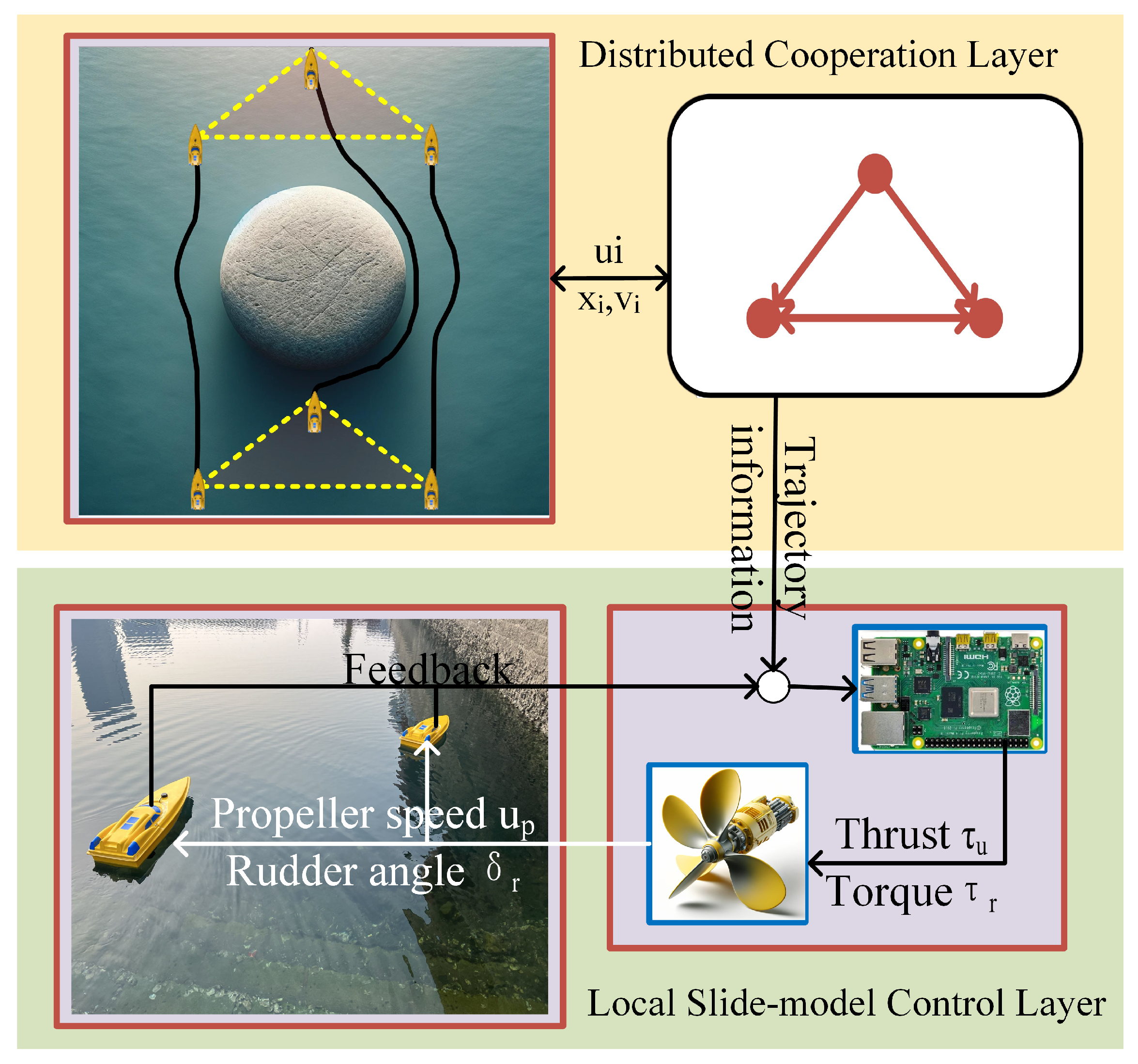
Due to the inherent complexity of directly applying the three-degree-of-freedom (3-DOF) motion model for coordinated control of unmanned surface vehicles (USVs), especially when multiple USVs are performing in surface coordinated movements, tight dynamic coupling issues are encountered. Furthermore, the single USV three-degree-of-freedom (3-DOF) motion model examined in this paper is under-actuated, meaning that the model has fewer control inputs than degrees of freedom (or state variables). This under-actuation presents challenges that must be addressed during the control process. To overcome these difficulties, inspired by [
29], this paper adopts a dual-layer USV fleet cooperative motion control framework, as shown in
Figure 1. The upper layer is the distributed cooperative layer; each vehicle in this layer is abstracted as a mass point with limited input driving force and motion speed, described by a second-order integrator motion model. Without considering the influence of wind, water flow, and the movement of other vehicles, the formation-containment task is completed by the distributed consistency control strategy, and the motion reference trajectory generated by each vehicle is transmitted to the lower layer. The lower layer is the local dynamic control layer, which employs the nonlinear sliding mode method [
29] to control the movement of an individual three-degree-of-freedom (3-DOF) unmanned surface vehicle (USV) motion model, performing real-time tracking based on the real-time reference trajectory generated by the corresponding vehicle in the upper layer. To achieve this objective, the three-degree-of-freedom dynamic model is employed. This model is described by the following equations, which delineate the motion of any unmanned vehicle
i within the cluster [
28]:
where
represents the position of vehicle
i’s center of gravity;
represents the heading angle of the vehicle;
,
, and
represent vehicle
i’s forward speed, sway speed, and yaw rate, respectively; “
,
, and
” represent the inertia parameters of vehicle
i in three coordinate directions, which can be calculated using a semi-empirical method; “
,
, and
” represent the components of the fluid damping experienced by vehicle
i on the water surface in three coordinate directions;
and
represent the control input forces of vehicle
i, which are thrust for forward motion and torque for turning, respectively.
Although the precise dynamic modeling of the lower control layer is crucial for overall system performance, this study primarily focuses on the upper layer, the distributed cooperative layer. Within this layer, the work presented here is dedicated to generating real-time reference trajectories for each unmanned surface vehicle (USV).
2.2. Graph Theory
The topology structure of
M USVs (unmanned surface vehicles) is often expressed by a digraph
, where
represents the set of nodes,
is the set of edges, and
stands for the adjacency matrix. It is assumed that
is an edge of
G, and there is a directed path from
to
if
. It is assumed that
if and only if
, and
otherwise. The neighbors of
i are represented by
, where
. Let diagonal matrix
, where
. Laplacian matrix
L is defined as
. If a root node has directional paths to all other nodes, the directional graph is said to contain a spanning tree. To illustrate the concepts mentioned above, the following
Table 1 provides an example to aid understanding.
2.3. Formation-Containment Tracking Task
The system composed by
USVs is considered. The USVs in the system can be divided into three categories, namely, the virtual leader or tracking leader, the real leaders or formation leaders, and the USV followers, as shown in
Figure 2. The reference trajectory for the macroscopic motion of the entire multi-USV system is generated through the virtual leader, which is numbered 0. And the real leaders, which are numbered
, are required to track the trajectory while completing the specified formation shape. Note that the formation shape in this paper is not time-varying. The followers need to converge to the convex hull formed by the real leaders, which are numbered
. The information exchange among USVs is described by digraph
G. The virtual leader has no neighbors, while a real leader can receive information from the virtual leader or the other real leaders, and a follower can receive information from the real leaders or the other followers.
The dynamics of the virtual leader in the distributed cooperative layer for the USVs can be expressed as follows, satisfying both the velocity and input constraints:
where
;
and
are the position vector and the velocity vector of the vitual leader;
is the desired velocity signal of the vitual leader; and
, where
and
are the minimum and the maximum values of the velocity of the virtual leader.
The dynamics of the
ith USV can be described by
where
,
, and
are the position vector, the velocity vector, and the control input vector for each agent, respectively. The formation of the real leaders can be described by
, where
.
represents the relative position vector between formation leader
i and the virtual leader.
Assumption 1. For directed graph G of the communication among virtual leader and real leaders, there is a spanning tree, and the root node is the tracking leader.
Assumption 2. For each follower, there is at least one real leader who can reach it through a directed path.
According to the topology characteristics of multi-USV systems, Laplacian matrix
can be represented as
where
,
,
, and
.
Let and , where if the virtual leader directly interacts with real leader i, or otherwise, and represents the Laplacian only among the real leaders, which ignores the virtual leader and the communication links it emits.
Let , where each represents the communication connection relationship between the ith real leader and all the followers. Similarly, let , where represents the Laplacian only among the followers, which ignores the real leaders and the communication links they emit, and each .
To facilitate the proof in the next section, the following lemmas and definitions are given.
Lemma 1 ([
40])
. If assumption 1 holds, then is of full rank. And there is a diagonal matrix , such that matrixes Q and satisfy , where . Lemma 2 ([
41])
. If assumption 2 holds, then is of full rank. There is a diagonal matrix , such that matrixes P and satisfy , where . Lemma 3 ([
42])
. If assumption 1 holds, then all eigenvalues of have positive real parts. Lemma 4 ([
43])
. If assumption 2 holds, then all eigenvalues of have positive real parts, and the sum of each row of equals 1. Additionally, every element of is non-negative. Definition 1. For the real leaders, ifthen the real leaders are considered to have completed the formation tracking task. Definition 2. For the followers, if there is a set of non-negative constants satisfying , and if the equationholds, then the followers are considered to have completed the containment task. Definition 3. If conditions (1) and (2) hold, then system (3) is considered to have completed the formation-containment tracking task.
Remark 1. In addition to the formation-containment tracking target, obstacle avoidance and collision avoidance are also the key concerns of the system in the process of completing the tasks. To ensure the normal execution of system tasks, firstly, a nominal controller which can perform the task of formation-containment tracking while constraining the input as well as the velocity of each USV is designed; secondly, various possible collisions will be presented as constraints to keep the system safe.
2.4. Collision Avoidance Using Control Barrier Function (CBF) Method
To ensure collision-free states in a dynamical system, we focus on systems of the form , where represents the system states and denotes the control inputs. Safety set S is defined using a zeroing control barrier function (ZCBF), which guarantees that the system states always remain within this set. Lemma 1 outlines the approach to achieve this goal.
Lemma 5 ([
39])
. For a given ZCBF candidate h that meets specific conditions, any Lipschitz continuous controller u: ensuring will maintain system states within safety set S and ensure asymptotic stability in d. Furthermore, to guarantee the forward invariance of safety set
S, the following inequality must be satisfied:
where
and
and
represent the Lie derivatives of
.
3. Main Results
In this section, a formation-containment tracking strategy based on neighbor information exchange is presented in part A. This controller is then constrained to avoid obstacles when necessary based on a control obstacle function in part B.
3.1. Formation-Containment Tracking Strategy
Lemma 6. We consider the following dynamic system:where . If the system satisfies the initial condition , then the constraint will hold all the time. At the same time, the acceleration of the system is also constrained. Proof. We suppose that the lemma is not true, which means that for a period of time . We assume that and . According to the Lagrange mean value theorem, there exists a time such that . However, since , we have . Therefore, the hypothesis is not valid. And ; by choosing , the acceleration of the system will be constrained. □
We consider the following nominal controller:
where
,
,
;
is the upper bound of the driving force;
and
represent the upper bound and the lower bound of the velocity of every single USV, respectively;
,
; and
represents the ultimate mean velocity.
Theorem 1. Based on Lemma 6, multi-USV system (2) can solve the formation-containment tracking problem while the system is constrained in velocity and input under protocol (8), where , , . Proof. First, the demonstration of the consistency between virtual leaders and real leaders is as follows.
The dynamic equation of Virtual Leader 0 is , where and ; it requires that and .
For the real leaders, we let
denote the error in the tracking formation.
Differentiating these two error quantities with respect to time
t yields
We let
and
and rewrite (
10) in vector form as
where
. We let
; then, it follows that
By moving the
term to the left side and letting
, it follows that
Then, we multiply both sides of (
13) by the
term and let
.
Matrix can be represented as , where . Due to , expresses the same virtual leader–real leaders communication connection as . By using Lemma 2, there are , which satisfy that and .
We consider the Lyapunov candidate function
. We differentiate the function along the trajectory of (
14) to obtain
where we use the fact that
. If
is equal to 0, then
is equal to 0. If not, then
, which means that
is equal to 0 in a finite time. Since
, it leads to
and
as
. And the system has completed the formation tracking task in a finite time. Then, it will be demonstrated that containment control can be achieved. For the real leaders, it follows that
, where
, which requires that
. For the followers, we let
denote the error in containment.
We let
and
. We rewrite (18) in vector form as
where
,
.
By substituting
into (19), it follows that
where
.
By rearranging the terms, we can derive
By letting
, it follows that
Matrix , where . Similarly, because of , expresses the same real leader–follower communication connection as . By using Lemma 3, there are , which satisfy that and .
Now, we consider the Lyapunov candidate equation
and differentiate the function along the trajectory of (
18) to obtain
We utilize the property of
, where each
. It derives
where we use the fact that
. If
is equal to 0, then
is equal to 0. If not, then
, which means that
is equal to 0 in a finite time. That means that
and
as
. And the system has completed the containment task. Thus, the formation-containment tracking problem is solved. □
Remark 2. The nominal controller of the system is designed by Lemma 6 to conform to the basic form where the velocities and control inputs are constrained. Real-time information exchange among the USVs is then used to achieve distributed control. To better alleviate to system jitters caused by nonlinear terms and to better achieve consistency, we may replace the sign function with (21) in practical applications. 3.2. Barrier Function-Based Collision Avoidance Controller
In the actual multi-USV system, the acceleration and velocity of USVs are limited. This should also considered in the distributed cooperation layer. Considering the difference between leaders and followers, it is assumed that the real leaders’ velocity () and acceleration () are limited by and , which means that and . Similarly, the followers’ velocity () and acceleration () satisfy and . The controller of each agent is designed as , where satisfies the control input of the safety set. Next, the security zone needs to be divided.
For convenience, the USVs and obstacles in the distributed cooperative layer are regarded as circles when dealing with obstacle avoidance and collision avoidance. Taking into account the difference between the USVs and the obstacles, it is supposed that the radius of the USVs is and that the radius of the ith obstacle is .
It is assumed that the safe distance among the USVs is , where . Considering the collision avoidance requirements, the distance between any two USVs must be satisfy all the time, where . For a pair of USVs i and j, where , the velocity difference can be expressed as .
The collision avoidance maintenance condition is converted into the forward invariance of some sets. A comprehensive consideration of possible collisions throughout the system has led to the classification of collisions into four scenarios.
Assumption 3. For each USV, the convergence position satisfies the safety distance requirement under a fixed topology. That means that , where , and .
- 1.
Case 1: First, we consider avoidance among the followers. According to the derivation similar to [
39], collision avoidance set of USV i can be expressed as
where
and
where
is the level set function of set
. This means that when a collision between two USVs is about to occur, each of the two USVs will prevent the collision with its maximum acceleration. Additionally, the forward invariance of
will be ensured if the ZCBF constraint in (
6) is satisfied. By combining (
6) and (
23), the following inequality can be obtained:
where
. It can also be written in the following form:
where
. Thus, we can constrain the safety barrier of USV
i and
j distribution as
Constraint (
25) can be written in the linear form
for each follower, where
and
.
- 2.
Case 2: Similarly, taking into account collision avoidance among real leaders, the following safety set can be obtained:
where
and
Then, the linear constraint can be obtained as for each real leader, where and . Since the virtual leader is not real, there is no need to consider its collision avoidance.
- 3.
Case 3: For a follower
i and a real leader
j, the collision avoidance set is
where
,
, and
The linear constraint can be obtained as , where and .
- 4.
Case 4: In addition to collision avoidance among USVs, collision avoidance between obstacles and USVs should also be taken into consideration. It is assumed that the safe distance between an USV i and an obstacle is , where . Considering the collision avoidance requirements, the distance between any USV and any obstacle must satisfy all the time.
First, considering collision avoidance between obstacles and followers, the safety set between a follower USV
i and an obstacle
is represented by the following expression:
where
and
where
is the level set function of set
. This means that when a collision between an USV and an object is about to occur, the USV will prevent the collision with its maximum acceleration. The velocity (
) and acceleration (
) of the obstacles can be detected by sensors mounted on the USV. Furthermore, the static obstacles can be regarded as special cases of the dynamic obstacles with zero velocity and acceleration. Additionally, the forward invariance will be ensured if the ZCBF constraint in (
6) is satisfied. By combining (
6) and (
28), the following inequality can be obtained:
Inequality (
29) can also be written in the following form:
where
. We let
stand for
; then, constraint (
30) can be written in the linear form
for each follower.
Then, considering the avoidance of collisions between a real leader j and obstacles, the following safety set can be obtained:
where
and
Then, we can obtain the linear constraint for each real leader, where .
In order to avoid collisions, the system needs to satisfy the constraints of the above four cases at all times. To ensure the effectiveness of the nominal controller, collision avoidance strategies should be triggered as little as possible, and the nominal controller should be modified as little as possible. Since the constraints are linear, the following quadratic programming (QP) problem can be formulated in a least squares sense:
where
,
is the nominal controller,
is the controller that satisfies the security strategy constraints,
L is the set of real leaders,
F is the set of followers, and
is the set of obstacles. The actual controller is shown in the following expression:
where
.
Theorem 2. Given the formation-containment tracking system, if for all USV , the control input is given by (33), where can be solved by QP problem (32), then the system is able to avoid collisions under assumption 3. Proof. If all controllers of the USVs satisfy the decentralized safety certificates, then security set
S is forward-invariant. If triggered, they are confined to the safety set [
39]. As a result, the system is able to achieve obstacle and collision avoidance. □
Remark 3. The priority of collision avoidance and obstacle avoidance control for USVs is higher than that of formation-containment control based on consensus for multiple USVs. When considering containment control problems, if the topology of the system is fixed, the final convergence position of the followers should be calculated in advance. If the final convergence position of the followers does not satisfy the safety distance requirement, the CBF (control barrier function) will take precedence in maintaining a safe distance between follower and follower, consequently disrupting the preset consensus formation among the followers. However, the pre-formed position of the real leader USV should satisfy the requirement of a safe position; otherwise, it may deviate from the preset trajectory due to the inability to achieve consistent velocity.
Remark 4. At this point, the conditions that the real leaders and followers need to meet to avoid obstacles and collisions have all been given. However, the proposed constraint takes into account all pairs of USVs, which can be a very large number. From a topology structure perspective, this requires all the information interactions of the USVs. With the increase in the number of USVs, the related computing and sensing requirements will increase significantly. We consider a fact that if the USVs are far away enough, they will not collide in a period of time. Thus, each USV i only needs to consider other USVs and obstacles in a certain range.
4. Simulation
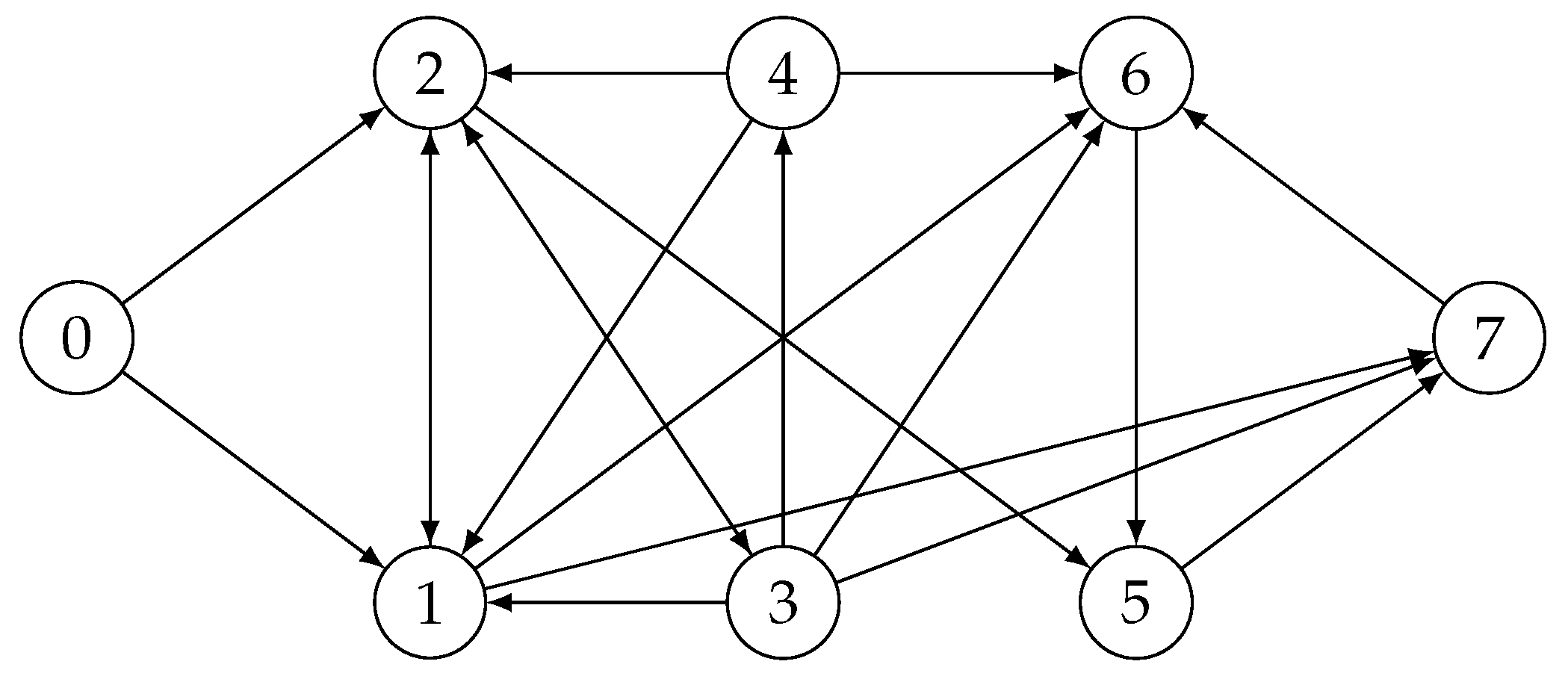
In this section, an example is used to illustrate the effectiveness of the control strategy in the distributed cooperation layer. The multi-USV system in this simulation example is composed of one virtual leader, four real leaders, and three followers. The communication topology of this system is shown in
Figure 3, where USV 0 is the virtual leader, USVs 1–4 are real leaders, and USVs 5–7 are followers. The initial position vector and initial velocity vector of USVs 1–7 are
and
, respectively. The formation shape given by the real leaders is a rectangle, and the specific value vector is
. The velocity limits of each real leader and follower are both
, and the input limits are both
. The dynamic equation of the virtual leader is
. The initial position vector and initial velocity vector of the virtual leader are
and
, respectively. And the velocity limits and acceleration limits given by the virtual leader are
and
, with
. According to Theorem 1, this leads to
. There is only one obstacle in the motion environment of the system. The radius of the USV in the distributed cooperative layer is 1 m, and the radius of the obstacle is 10 m. This means that the safe distance among USVs is 2 m and the safe distance between any USV and any obstacle is 11 m.
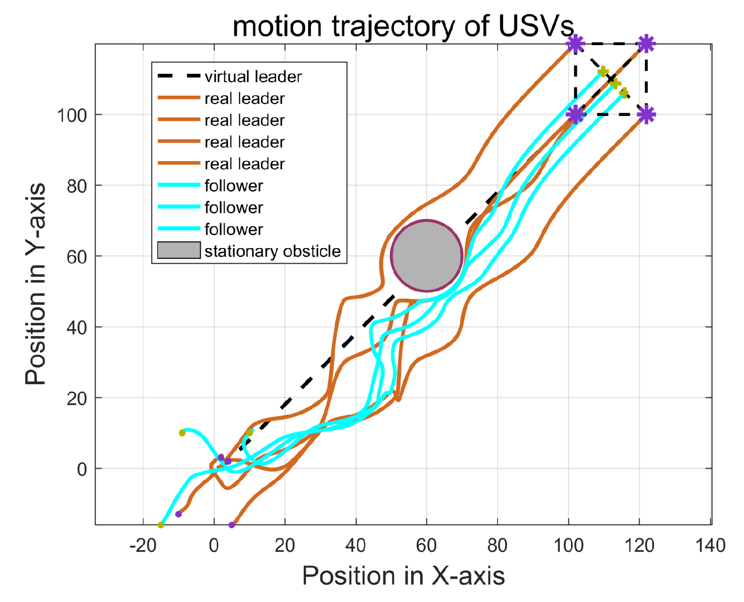
The trajectories of USVs in the distributed cooperative layer obtained by the multi-USV system driven by controller (33) are shown in
Figure 4. The system can be driven by the control strategy to perform the formation-containment tracking control task: real leaders can form the expected formations; followers can converge into the convex hull; the motion of the whole system is controlled by the virtual leader. At the same time, all USVs can avoid obstacles. The smooth trajectories of the agents represent no significant abrupt changes in the state of the USVs.
More details on three aspects are presented in the following simulation: the implementation of formation-containment tracking, the velocities and input constraints of the USVs, and the effectiveness of the obstacle and collision avoidance strategy.
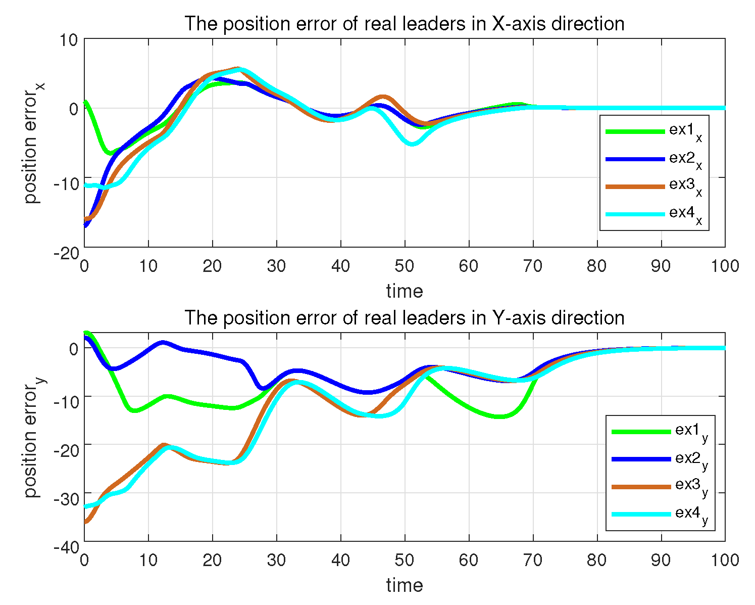
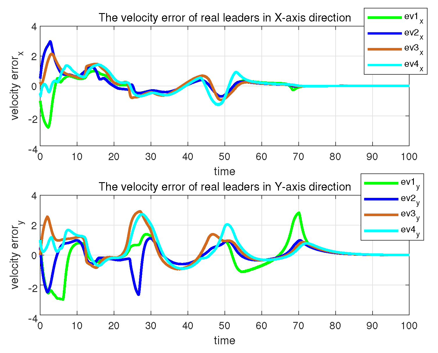
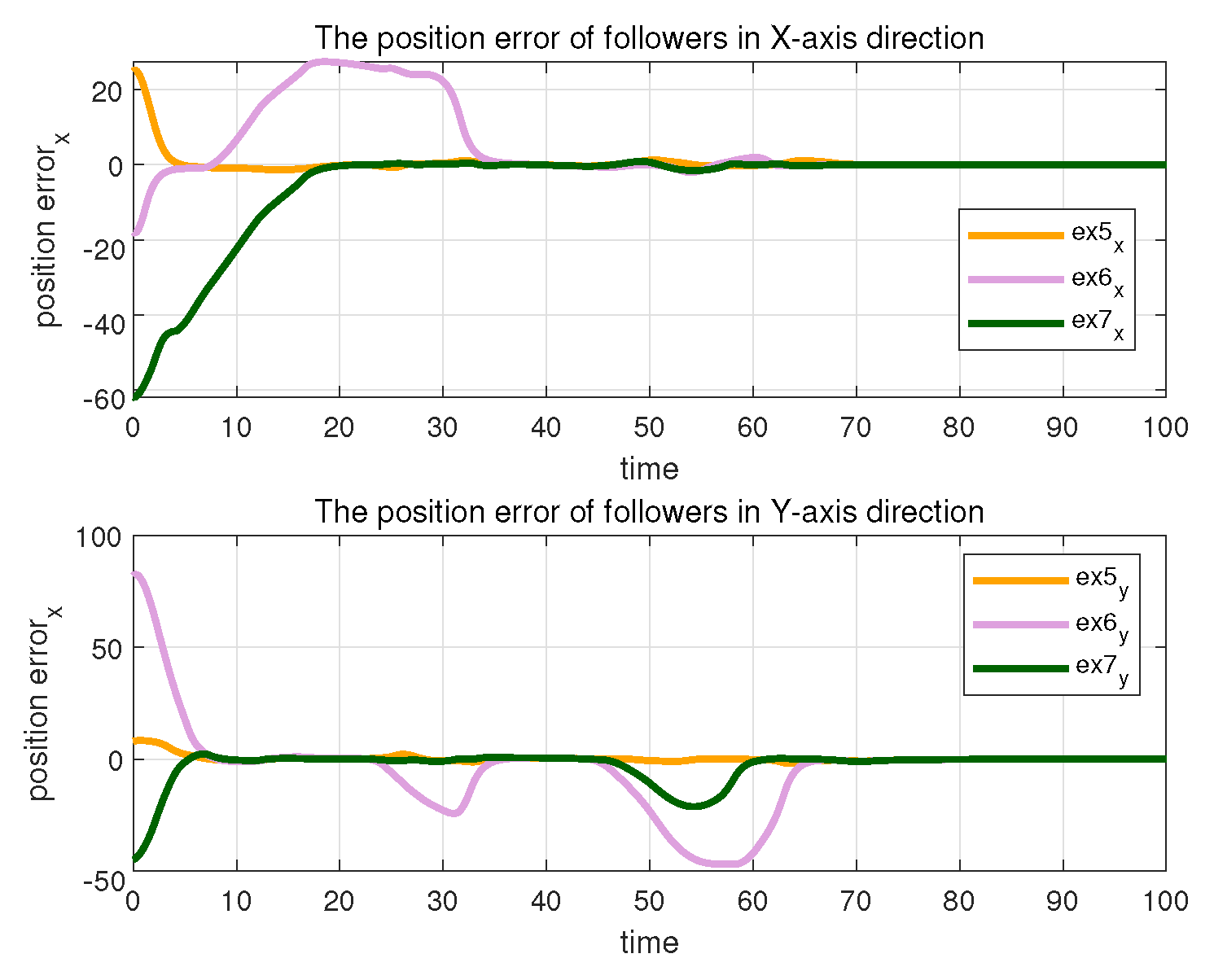
The errors in formation-tracking control and containment control can be seen in
Figure 5,
Figure 6,
Figure 7 and
Figure 8.
Figure 5 and
Figure 6 show the formation-tracking position errors and velocity errors of the real leaders. The errors arise from the need for real leaders to track virtual leader states and form time-invariant formations, as shown in Equation (
9).
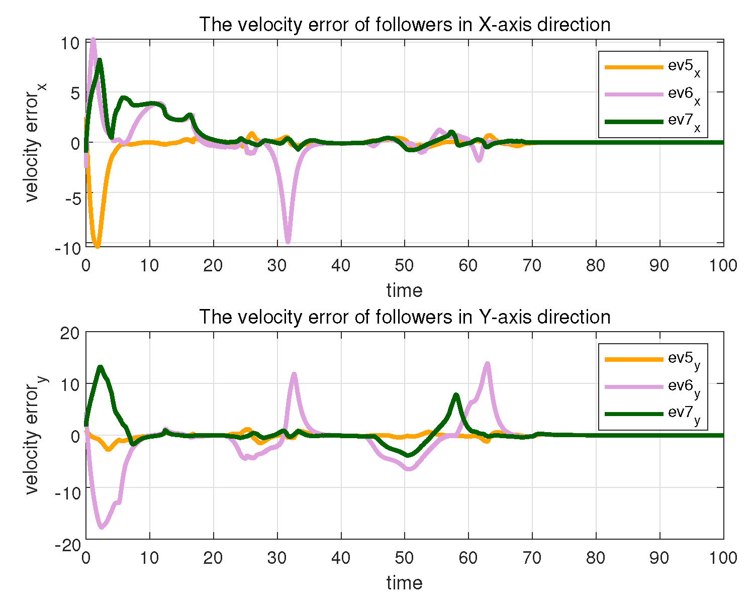
Figure 7 and
Figure 8 show the containment position errors and velocity errors of the followers. The errors arise from the need for followers to track the states of the real leaders, as shown in Equation (
16). The asymptotic convergence of all errors to zero indicates that the system is finally stable and completes the formation-containment tracking control task. The oscillations in these figures are produced by avoiding obstacles and other USVs. It is worth noticing that the convergence of the followers occurs after the convergence of the real leaders, but the time interval can be ignored in the application of the algorithm.
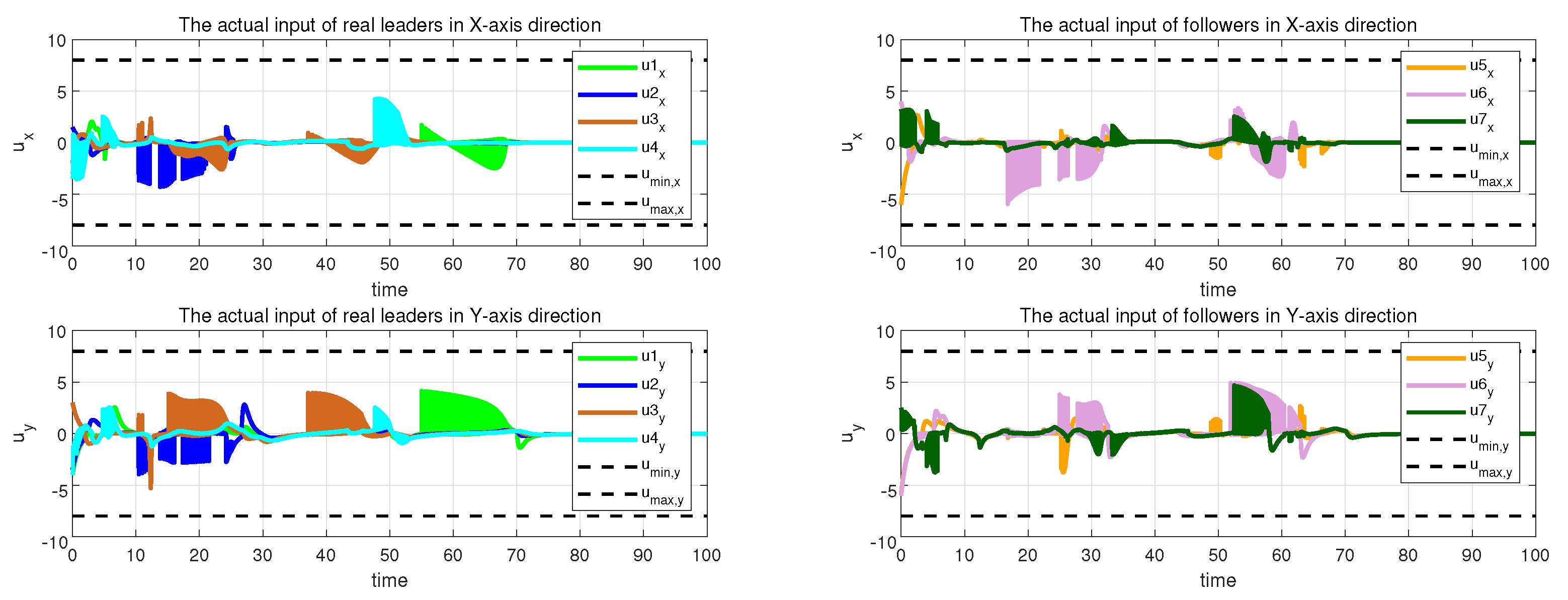
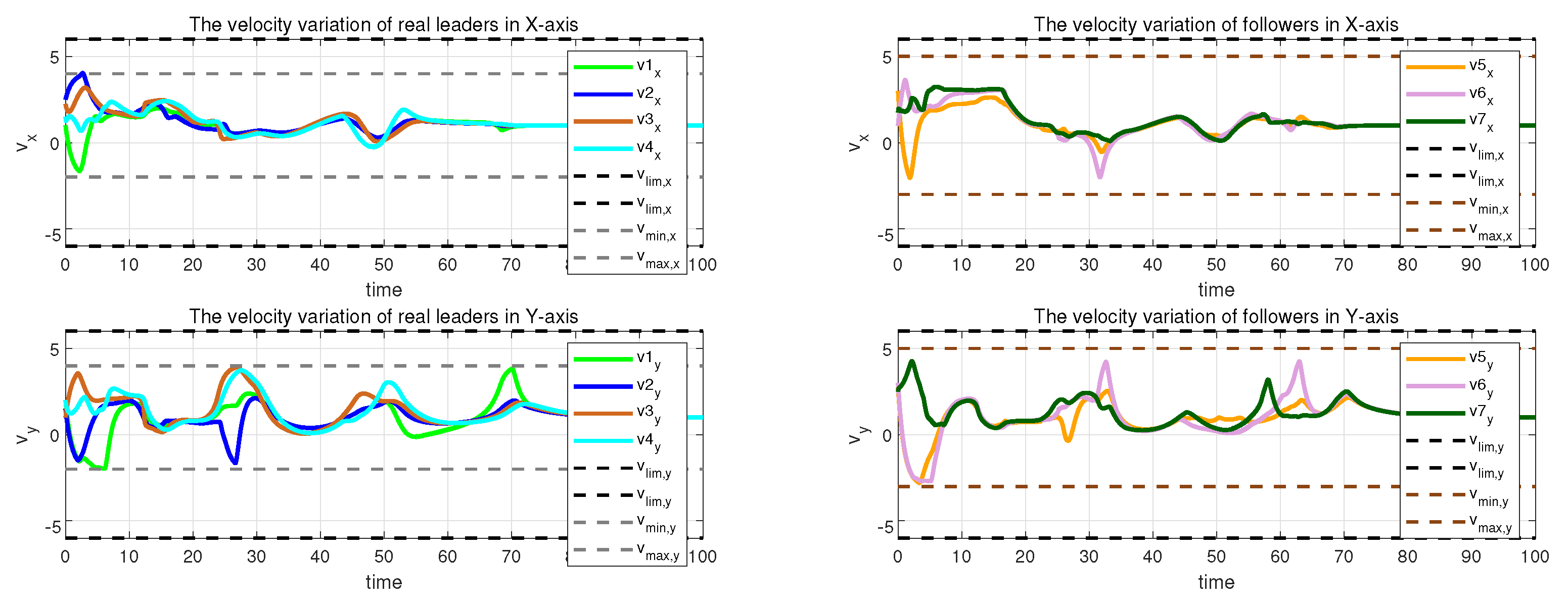
The accelerations and velocities of each USV are limited to the required range, as shown in
Figure 8 and
Figure 9, where dashed lines indicate acceleration and velocity limits. Although the controller input oscillates during obstacle avoidance, the velocities and accelerations of all USVs eventually converge to the same level. The oscillations are caused by the controller solving a quadratic programming problem during obstacle avoidance, the solution of which leads to abrupt changes in the controller inputs. Even during the obstacle avoidance process, the velocities and accelerations of all the USVs do not exceed the required limits.
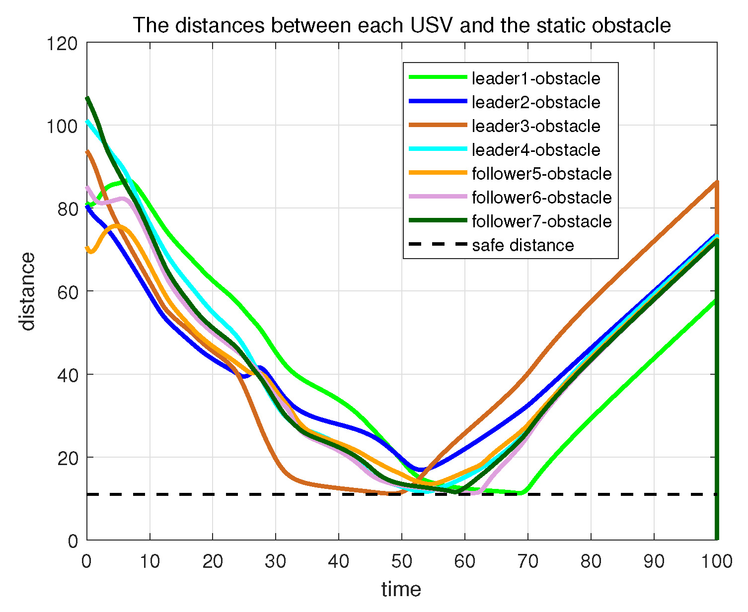
To illustrate more clearly that in this example, the USVs can avoid obstacles, the distance between each USV and the center of the obstacle is plotted, as shown in
Figure 10, where the dashed lines represent the safe distance. We further illustrate the effectiveness of obstacle avoidance by adding a time axis, zooming in on the local trajectory figure, and increasing the safety distance incrementally, as shown in
Figure 11. The figure shows that the trajectory of each USV is smooth when avoiding obstacles and confirms that the velocities and inputs of each USV are limited. With the increase in safety distance, the implementation of the algorithm is still effective. Therefore, in practice, the setting of safety distance can be adjusted appropriately for better security.
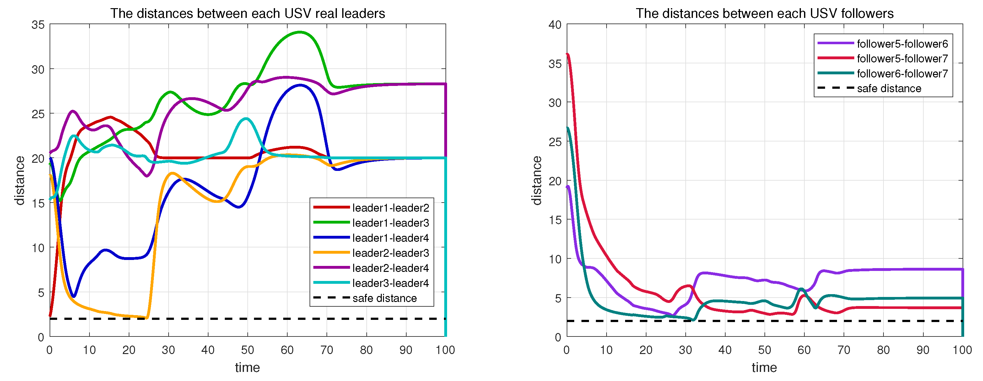
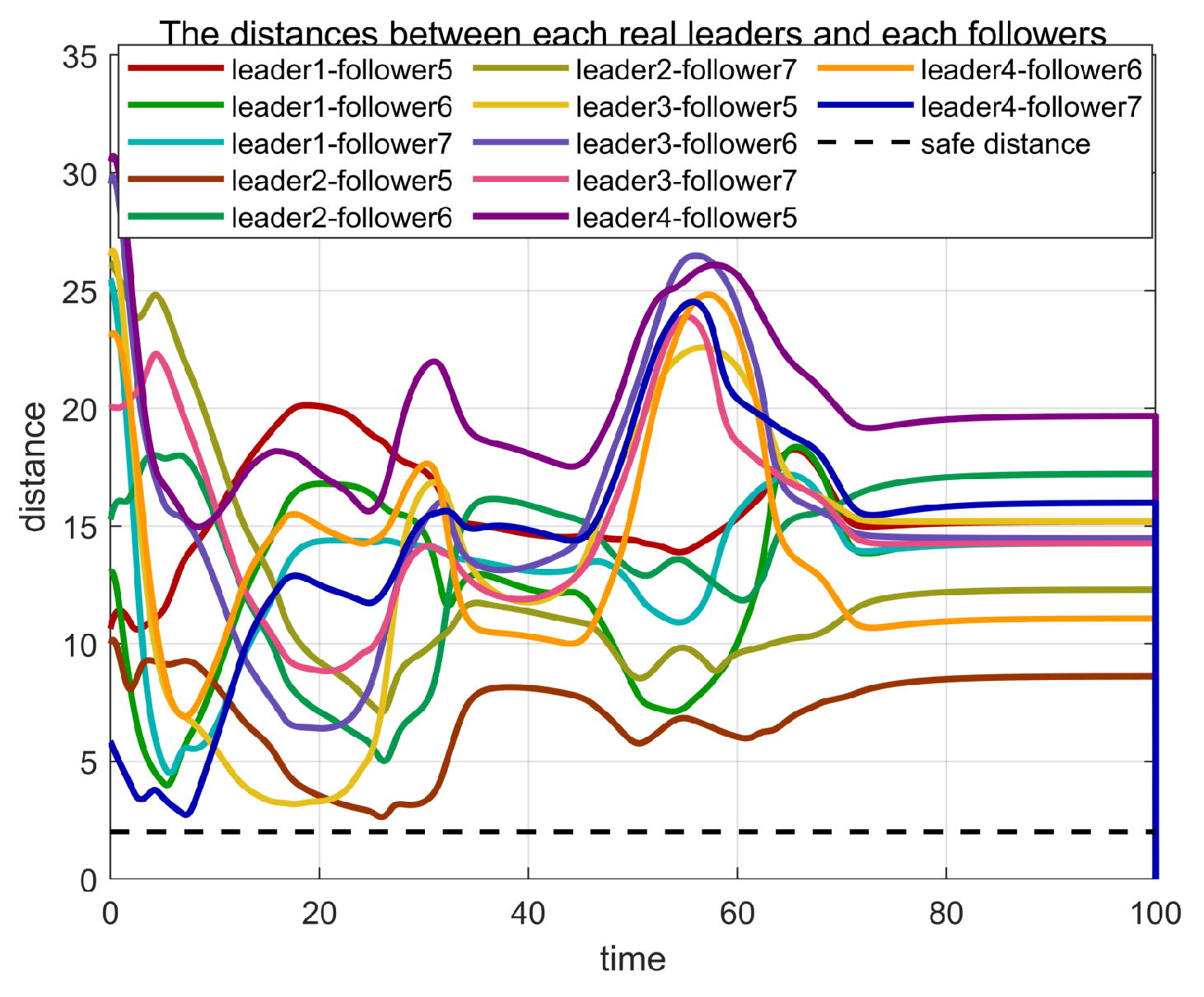
Due to the different limited accelerations and velocities of the followers and leaders, the distance between the USVs is plotted to illustrate the collision avoidance effectiveness of the USVs, as shown in
Figure 12 and
Figure 13, with the dotted line representing the safe distance. In this example, the initial position of the real leader is set farther away from the follower, and the likelihood of collisions occurring is reduced. However, the whole system still realizes collision avoidance with the USVs avoiding obstacles.


