A Novel, Finite-Time, Active Fault-Tolerant Control Framework for Autonomous Surface Vehicle with Guaranteed Performance

Abstract

In this paper, a finite-time, active fault-tolerant control (AFTC) scheme is proposed for a class of autonomous surface vehicles (ASVs) with component faults. The designed AFTC framework is based on an integrated design of fault detection (FD), fault estimation (FE), and controller reconfiguration. First, a nominal controller based on the Barrier Lyapunov function is presented, which guarantees that the tracking error converges to the predefined performance constraints within a settling time. Then, a performance-based monitoring function with low complexity is designed to supervise the tracking behaviors and detect the fault. Different from existing results where the fault is bounded by a known scalar, the FE in this study is implemented by a finite-time estimator without requiring any prioir information of fault. Furthermore, under the proposed finite-time AFTC scheme, both the transient and steady-state performance of the ASV can be guaranteed regardless of the occurrence of faults. Finally, a simulation example on CyberShip II is given to confirm the effectiveness of the proposed AFTC method.

1. Introduction

In recent years, significant progress has been made in the field of marine autopilots, which has attracted a great deal of attention. An important area of research in this field is the control of autonomous surface vehicles (ASVs). The ability of ASVs to operate in remote and hazardous areas, coupled with their advanced sensing and control capabilities, make them valuable assets for various applications in the marine, research, and exploration industries. Numerous successful results have been developed for the control of ASVs, such as [1,2,3,4,5,6,7]. The authors of [1,2] presented a comprehensive literature review of the recent progress in ASVs’ development, and highlighted more general challenges and future directions of ASVs towards more practical guidance, navigation, and control capabilities. Common issues encountered in ASV control include trajectory tracking [3,4,5], formation control [6], and cooperative target tracking control [7]. These positive results have led to widespread applications of ASVs in marine environments, encompassing complicated tasks such as ocean forecasting, surface inspection, and pipeline tracking. However, The presence of unpredictable factors such as rough waves, strong currents, and changing weather conditions can adversely affect the performance and integrity of the ASV system. specifically, the intricate and dynamic nature of the surface environment poses significant challenges to the reliable operation of various components within the ASV system, including sensors, actuators, and controllers. This complexity substantially increases the susceptibility of these components to potential malfunctions [8]. Furthermore, the repair of these components during operation is impractical [9]. This introduces significant safety risks for ASVs, making safety control a primary concern in fulfilling the vehicle’s mission. It becomes crucial to develop robust and resilient designs that can deal with these environmental risks and ensure the continued functionality of ASVs in demanding marine conditions. Confronting this challenge, fault-tolerant control (FTC) methods have been proposed to enhance the safety and reliability of ASVs, maintaining stable operation and eliminating the effects of system malfunctions [10,11,12,13,14].

Fault-tolerant control schemes are classified as passive fault-tolerant control (PFTC) and active fault-tolerant control (AFTC), depending upon the utilization of fault detection and diagnosis module and the implementation of redundancies [15]. In PFTC methods, a fixed controller was designed that maintains the stability and performance of the control system during both normal and faulty operating situations [16,17,18]. The fixed controller is pre-designed with system redundancies which can be invoked, such as switching to backup components or adjusting operational parameters to compensate for the fault. PFTC approaches can ensure that the control system remains stable and performs well even in the presence of faults, without requiring any significant changes to the control structure. In an AFTC system, the controller reacts to malfunctions in system components through the controller reconfiguration, guided by detection information generated by the fault detection (FD) module. Once a fault is detected, the AFTC scheme determines the most effective strategy for maintaining system stability and performance. For the controller reconfiguration, the AFTC system dynamically adjusts the control parameters, modifies the control laws, or redistributes control tasks among redundant components to eliminate the effects of the fault. In comparison, PFTC methods are typically simpler to implement and require less computational resources than AFTC techniques, making them a practical solution for the control system. On the other hand, AFTC methods are more complex and computationally demanding compared to PFTC methods but can offer greater flexibility and adaptability in responding to faults. By actively reconfiguring the control, AFTC techniques can effectively overcome faults and maintain system functionality, making them suitable for applications where immediate fault response and system optimization are critical.

As a result, AFTC schemes have attracted significant attention in research and engineering applications due to their flexibility and accuracy [19,20,21]. In [19], the authors proposed a distributed AFTC approach for satellite formation flying attitude control, where sensor errors can be diagnosed by nonlinear observers and static approximators. A novel AFTC scheme was proposed in [20] for uncertain fully actuated systems using the integrated integration structure with observer and controller to reveal the model characteristics, which include faults and uncertainty. In [21], an observer-based AFTC algorithm was designed for spacecraft with full state constraints, and the fault diagnosis was implemented by a linear matrix inequality (LMI)-based robust fault observer. Nevertheless, despite the advantages offered by AFTC methods, there are some issues with the aforementioned studies that require further investigation: (1) The utilization of an ideal data model in the FD makes it difficult to adapt and implement in real systems, and (2) the convergence time of the fault observer has not been considered to ensure the accurate and efficient estimation. Consequently, there is a pressing need to develop an AFTC scheme integrating implementable FD and precise fault estimation (FE) to guarantee the reliable tracking control of ASVs.

As a critical component of AFTC systems, FD has garnered significant attention in recent years, and researchers have published various meaningful results [22,23,24]. The integration of FD mechanisms plays a crucial role in enhancing the reliability and robustness of control systems, especially in the presence of component faults. By accurately identifying faults, the control systems can effectively adapt their control strategies to mitigate potential disruptions and ensure safe operation in dynamic environments. In [24], the authors introduced a robust FE strategy that relies on residual generation and evaluation modules. This approach enables the identification of fault occurrence, characteristics, and severity by analyzing input and state information. When the residual evaluation function surpasses the predefined threshold level, a fault is detected, triggering the generation of an alarm signal. It is worth mentioning that disturbance observation (DO) algorithms can provide many ideas and references for FD because of the similar uncertainty characteristics between disturbance and component fault. Until now, the control of surface and underwater vehicles has shown a wider range of achievements with DO as opposed to FD [25,26,27]. In [26], a fast estimation method was developed to assess the real-time evolution of wave disturbances acting on a vehicle and verified by incorporating the predicted loads within a Model Predictive Controller. An integrated deterministic sea wave predictor was proposed for underwater vehicles in [27], demonstrating high potential to effectively mitigate disturbances and facilitate accurate tracking performance even in the presence of high wave loading. These results offer valuable insights for the development of FD design. For example, an interval observer was constructed in [28] to detect and isolate the faults in multi-agent systems by generating the residual signals and implying the thresholds. In [29], the faults were detected by an adaptive interval observer, and isolated by a set of interval observers. However, ASVs operate in complex marine environments and are inevitably subject to high operational risks, failure types cannot be identified, and certain bounds of faults cannot be given. Although many scholars have devoted themselves to design thresholds and estimate the faults, the fault detection for ASV systems is still an open research problem.

From a practical perspective, the primary responsibility of ASVs is to maintain tracking performance, and fulfill their designated tasks accurately, reliably, and adaptively. To address this, several advanced control techniques have been employed in recent studies. These studies, referenced as [30,31,32,33,34], have explored different control strategies to enhance the tracking capabilities of ASVs in terms of accuracy, stability, and adaptability, enabling them to fulfill their tracking responsibilities effectively. Transient (convergence rate, overshoot, and undershoot) and steady-state performances are important performance metrics that should be considered for control systems. Considering these performance metrics is essential in evaluating the effectiveness of control strategies. For this purpose, a novel control method known as prescribed performance control, introduced in [35], has achieved plenty of positive results when applied to multiple control systems [36,37,38]. Prescribed performance control focuses on achieving specific performance objectives while ensuring robustness against uncertainties and disturbances. Due to this property, prescribed performance control algorithms have been designed for surface vessels in [39,40] to achieve the assigned trajectory mission. Building upon the concept of [35], a novel concept known as finite-time performance function (FTPF) was presented in [41], which achieves finite-time convergence while ensuring the transient and steady-state performances. An FTPT-based fuzzy adaptive controller was developed in [42] for the trajectory tracking problem of multiple input multiple output nonlinear systems to ensure the tracking error has the predefined performance in finite time. In [43], the FTPF was utilized to design an air–ground cooperative consensus control scheme by integrating with the fixed-time scheme, which can guarantee the predefined time and given formation performance simultaneously. However, maintaining and restoring the guaranteed performance becomes more notably challenging when faults occur in ASVs. Therefore, it is significant to develop an AFTC scheme for ASV that can both detect faults and maintain predefined performance, while ensuring safety and reliability in the whole operating process. However, when faults occur in ASVs, maintaining and restoring the guaranteed performance becomes notably more challenging. Therefore, it is crucial to develop an AFTC scheme for ASVs that can detect faults and maintain predefined performance while ensuring safety and reliability throughout the entire operating process. By integrating the FTPF with the AFTC scheme, it is possible to achieve both predetermined performance objectives and fault tolerance capabilities in ASVs. This integration allows for effective tracking and control of ASVs, even in the presence of faults or disturbances.

Motivated by the above discussion and observation, in this paper, we aim to develop an AFTC scheme for ASV with a predefined finite-time tracking performance guaranteed. By incorporating the FTPF and Barrier Lyapunov function, a nominal controller is proposed to maintain the performance under normal conditions, and a fault monitoring function is obtained to achieve fault detection in time. Once the fault is detected, a reconfigured controller with a finite-time estimator is employed to ensure the predefined performance is guaranteed all the time. The main characteristics and contributions are summarized as follows:

(1)

The paper makes the first attempt to develop an integrated FD, FE, and FTC framework for ASV. Through the utilization of transformed performance constraints, a monitoring function with low complexity is formulated to supervise system behavior and facilitate fault detection. This approach eliminates the need for intricate threshold calculations as seen in existing works such as [44,45,46].

(2)

The concept of FTPF is first introduced to solve the fault-tolerant problem of ASVs. A nominal controller and a reconfigured controller are proposed by integrating the FTPF and Barrier Lyapunov functions. Using the proposed controllers, the tracking errors are guaranteed within a specified performance metric in a settling time.

(3)

To enable efficient controller reconfiguration, a finite-time estimator is designed to accurately estimate uncertainties and faults. In comparison to previous works such as [20,21,44], the proposed estimator does not require a priori knowledge of the upper bound of the fault.

The remaining part of the paper is organized as follows. In Section 2, the system modeling and essential knowledge are introduced. The nominal controller and the reconfigured controller design process are given in Section 3. In Section 4, the simulation result is presented to illustrate the effectiveness of the designed controllers. The conclusion is clarified in Section 5.

Throughout this paper, the following notations are adopted. $\mathbb{R}$ is the set of all real numbers, and ${\mathbb{R}}^n$ represents the Euclidean space with dimension n. For a vector $x\in {\mathbb{R}}^n$, $x_i(i=1,2,...,n)$ means the corresponding ith component of x, ${\lambda }_{max}\left(x\right)$ and ${\lambda }_{min}\left(x\right)$ mean the minimum and maximum eigenvalues, respectively. $|·|$ denotes the absolute value of a scalar, $\parallel ·\parallel$ denotes the Euclidean norm of a vector, diag$(·)$ is a diagonal matrix. $I_{n\times n}$ denotes an identity matrix of dimension n.

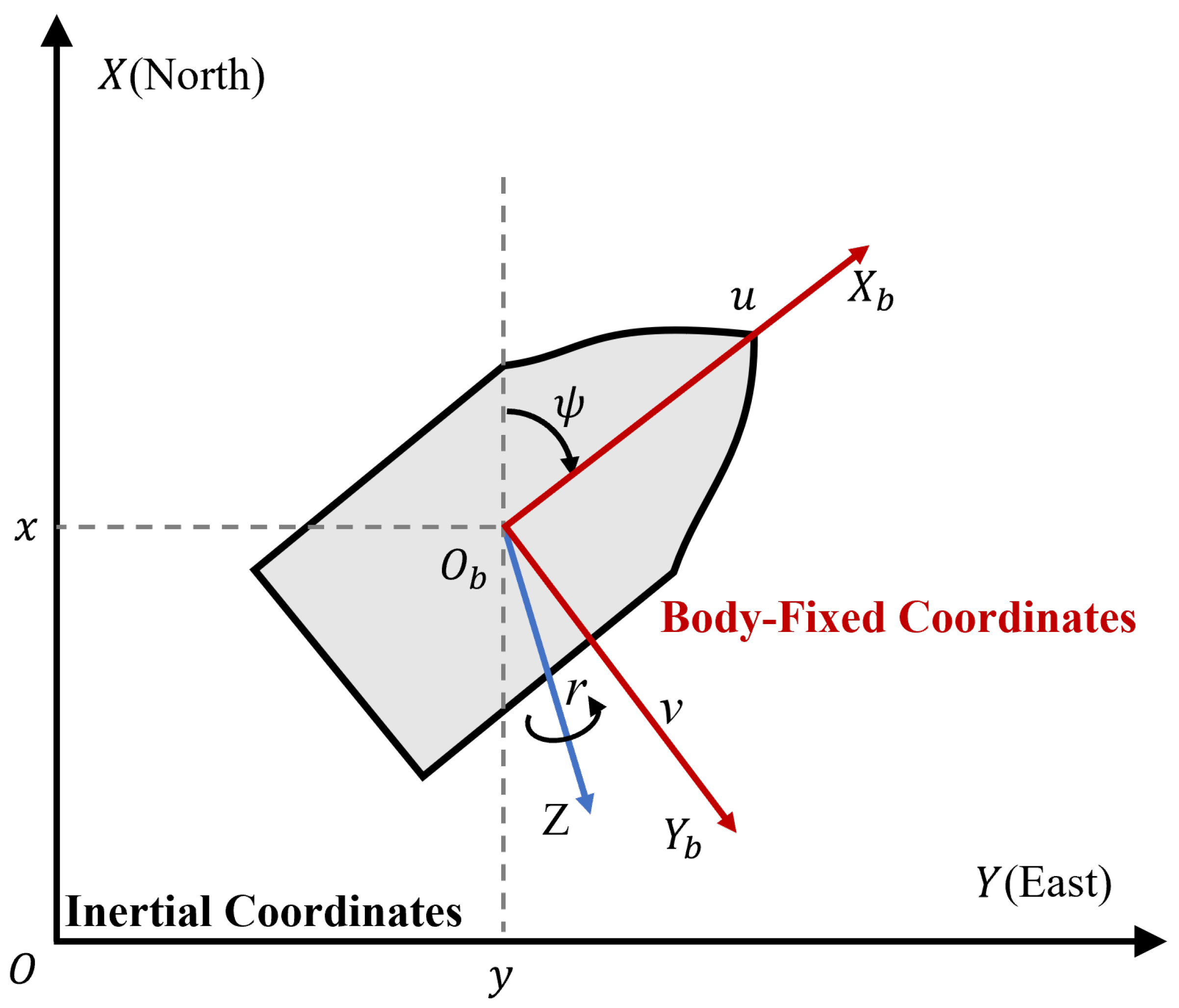
2. Problem Formulation and Preliminaries

2.1. Problem Statement

The standard three degrees of freedom (DOF) model of the ASV under two right-hand coordinate systems is considered, as illustrated in Figure 1. According to the trajectory tracking mission of ASV, the nonlinear motion equation of the vehicle in the horizontal planes can be described as

$$\begin{array}{cc}\hfill & \dot{\eta }=R\left(\eta \right)\nu ,\hfill \\ \hfill & M\dot{\nu }+C\left(\nu \right)\nu +D\left(\nu \right)\nu +d\left(t\right)=\tau +{\tau }_d,\hfill \end{array}$$

(1)

where $\eta ={[x,y,\psi ]}^T\in {\mathbb{R}}^3$ describes the position and yaw angle of the vehicle represented in inertial coordinates, and $\nu ={[u,w,r]}^T\in {\mathbb{R}}^3$ is the surge, sway, and yaw velocities represented in body-fixed coordinates. The rotation matrix between two coordinates is expressed by

$$R\left(\eta \right)=\left[\begin{array}{ccc}\cos \left(\psi \right)& -\sin \left(\psi \right)& 0\\ \sin \left(\psi \right)& \cos \left(\psi \right)& 0\\ 0& 0& 1\end{array}\right].$$

(2)

For simplicity, $R\left(\eta \right)$ is denoted as R in the following. It can be found that the determinant of (2) is positive, so R is invertible. The matrix $M=M^T\in {\mathbb{R}}^{3\times 3}$ denotes the inertial matrix, $C\left(\nu \right)\in {\mathbb{R}}^{3\times 3}$ describes the Coriolis and centripetal matrix, $D\left(\nu \right)\in {\mathbb{R}}^{3\times 3}$ represents the nonlinear damping matrix, $d\left(t\right)\in {\mathbb{R}}^3$ denotes the unmodeled dynamics, and ${\tau }_d\in {\mathbb{R}}^3$ is the unknown disturbance from wind, wave, and marine currents. The control forces and torque are given by $\tau \in {\mathbb{R}}^3$.

Using the conversion relation between $\eta$ and $\nu$, we have

$$\begin{array}{cc}\hfill \dot{\eta }=R\nu & \iff \nu =R^{-1}\dot{\eta }\hfill \\ \hfill \ddot{\eta }=\dot{R}\nu +R\dot{\nu }& \iff \dot{\nu }=R^{-1}(\ddot{\eta }-\dot{R}{R}^{-1}\dot{\eta }).\hfill \end{array}$$

(3)

Based on (3), the ASV model (1) under the fault-free condition is rewritten by

$$\begin{array}{cc}\hfill \ddot{\eta }=& \dot{R}{R}^{-1}\dot{\eta }-R{M}^{-1}(C(\eta ,\dot{\eta })+D(\eta ,\dot{\eta }))R^{-1}\dot{\eta }+R{M}^{-1}\tau +R{M}^{-1}({\tau }_d-d).\hfill \end{array}$$

(4)

The challenging operating conditions of ASVs increase the possibility of malfunctions in sensors, actuators, and controllers. In this paper, fault represents a state where a system or component does not meet its intended function or performance requirements. Specifically, a component fault refers to a failure or malfunction of an individual component within a control system, such as a sensor, actuator, controller, or any other hardware or software element involved in the control process. According to [20], the bias component faults can be modeled as $f_a\in {\mathbb{R}}^3$, satisfying ${sup}_{t\in [0,\infty ]}\parallel f_a\parallel <\infty$ and ${sup}_{t\in [0,\infty ]}\parallel {\dot{f}}_a\parallel <\infty$. In practice, it is challenging to determine the upper bounds of component faults due to the complex failure modes of ASVs. According to [47], the possible transition from the fault-free case to the fault case is unidirectional. Furthermore, we also assume that the fault occurred once during operation. Then, the faulty ASV model with the general component fault is considered as

$$\begin{array}{cc}\hfill & \dot{\eta }=R\left(\eta \right)\nu ,\hfill \\ \hfill & M\dot{\nu }+C\left(\nu \right)\nu +D\left(\nu \right)\nu +f_a+d=\tau +{\tau }_d,\hfill \end{array}$$

(5)

The control objective of this paper is to develop an integrated finite-time AFTC framework for ASV so that the fault can be detected and estimated precisely, and the predefined tracking performance is ensured under both fault-free and faulty cases.

Assumption 1. 

The desired trajectories ${\eta }_d$ along with their time derivatives ${\dot{\eta }}_d$, ${\ddot{\eta }}_d$ are smooth and bounded.

Assumption 2. 

The external disturbance ${\tau }_d$ is bounded, i.e., there is a positive constant ${\overline{\tau }}_d$, such that $\parallel {\tau }_d\parallel \le {\overline{\tau }}_d$.

Assumption 3. 

Under normal operation of ASV, the unmodeled dynamics $d\left(t\right)$ is bounded by $\parallel d\left(t\right)\parallel \le \overline{d}$ with $\overline{d}$ being a conservative constant.

Lemma 1 

([41]). Given a function $\phi \ge 0$ and

$$\frac{d\phi \left(t\right)}{dt}=-\iota {\left[\phi \left(t\right)\right]}^{\kappa }$$

(6)

holds, where $\iota >0$ and $0<\kappa <1$ are the constants. Then (6) can be solved for

$$\phi \left(t\right)=\left\{\begin{array}{c}\begin{array}{cc}{\left({\left(\phi \left(0\right)\right)}^{1-\kappa }-(1-\kappa )\iota t\right)}^{\frac{1}{1-\kappa }},\hfill & \hfill t\in [0,T_0)\\ 0,\hfill & \hfill t\in [T_0,+\infty )\end{array}\end{array}\right.$$

(7)

where $T_0=\frac{{\left(\phi \left(0\right)\right)}^{1-\kappa }}{\iota (1-\kappa )}$.

2.2. Finite-Time Performance Function

In this subsection, we introduce the definition of FTPF, which aims at achieving two goals: first, it serves as a criteria for establishing a fault detection mechanism to identify component faults. Secondly, it ensures that tracking errors converge to the small specified residual sets within a settling time interval, even if fault occurs.

The definition of FTPF is as follows.

Definition 1 

([41]). A function $\rho \left(t\right)$ is designated as the FTPF when it exhibits these properties:

• $\rho \left(t\right)>0$;
• $\dot{\rho }\left(t\right)\le 0$;
• ${lim}_{t\to T_s}\rho \left(t\right)={\rho }_{T_s}>0$;
• $\rho \left(t\right)={\rho }_{T_s},\forall t\ge T_s$ with $T_s$ being the settling time.

From Definition 1, it can be observed that $\rho \left(t\right)$ can converge to a specified set within the settling time $T_s$, indicating that $\rho \left(t\right)$ converges in finite time. According to Lemma 1, the FTPF employed in this paper is chosen as

$${\rho }_i\left(t\right)=\left\{\begin{array}{c}\begin{array}{cc}{({\rho }_{i0}^{\epsilon }-\iota \epsilon t)}^{\frac{1}{\epsilon }}+{\rho }_{i{T}_s},\hfill & \hfill t\in [0,T_s)\\ {\rho }_{i{T}_s},\hfill & \hfill t\in [T_s,+\infty )\end{array}\end{array}\right.$$

(8)

where $i=1,2,3$, ${\rho }_{i0},{\rho }_{i{T}_s},\iota \in \mathbb{R}$ are positive constants to be chosen, $\epsilon =\frac{{\epsilon }_1}{{\epsilon }_2}\in (0,1]$ with ${\epsilon }_1,{\epsilon }_2$ are positive odd integers. Based on (8), the settling time $T_s$ can be calculated by $T_s=\frac{{\rho }_0^{\epsilon }}{\iota \epsilon }$.

2.3. Error Transformation

In this subsection, the performance constraints for the tracking error is given first. Then, an error transformation is presented to transfer the time-varying constraints into an equivalent constant one to facilitate the design of AFTC scheme.

To achieve the control target, the ASV is requested to track the reference trajectories with guaranteed performance, which indicates that the tracking error $e=\eta -{\eta }_d$ should satisfy

$${\underline{\rho }}_i\left(t\right)<e_i\left(t\right)<{\overline{\rho }}_i\left(t\right),$$

(9)

where $i=1,2,3$, ${\underline{\rho }}_i$ and ${\overline{\rho }}_i$ represent the lower and upper constraints, respectively. Suppose $e_i\left(0\right)$ satisfies ${\underline{\rho }}_i<\left|e_i\left(0\right)\right|<{\overline{\rho }}_i$, depending on the sign of $e_i\left(0\right)$, the following should hold:

$$e_i\left(0\right)\ge 0:\left\{\begin{array}{c}\begin{array}{cc}\hfill {\underline{\rho }}_i& =-{\sigma }_i{\rho }_i\left(t\right)\hfill \\ \hfill {\overline{\rho }}_i& ={\rho }_i\left(t\right)\hfill \end{array}\end{array}\right.,e_i\left(0\right)<0:\left\{\begin{array}{c}\begin{array}{cc}\hfill {\underline{\rho }}_i& =-{\rho }_i\left(t\right)\hfill \\ \hfill {\overline{\rho }}_i& ={\sigma }_i{\rho }_i\left(t\right)\hfill \end{array}\end{array}\right.,$$

(10)

where ${\rho }_i\left(t\right)$ is the FTPF given in (8), ${\sigma }_i$ is the design parameter.

Then, a sufficient necessary condition is deduced to ensure that the guaranteed performance described in (9) is achieved. The error transformation technology introduced and employed to convert the complex bounds (8) into more concise bounds as

$$z_i\left(t\right)=T_i(e_i\left(t\right),{\underline{\rho }}_i\left(t\right),{\overline{\rho }}_i\left(t\right)),i=1,2,3.$$

(11)

where $z={[z_1,z_2,z_3]}^T\in {\mathbb{R}}^3$ denotes the transformed error. According to [35], the given attributes should be present in the error transformation function $T_i(·)$:

• $T_i(·)$ is smooth and strictly increasing;
• ${lim}_{e_i\to {\overline{\rho }}_i}{T}_i(e_i\left(t\right),{\underline{\rho }}_i\left(t\right),{\overline{\rho }}_i\left(t\right))=1$;
• ${lim}_{e_i\to {\underline{\rho }}_i}{T}_i(e_i\left(t\right),{\underline{\rho }}_i\left(t\right),{\overline{\rho }}_i\left(t\right))=-1$.

Following these considerations, the error transformation function is designed as

$$T_i(e_i\left(t\right),{\underline{\rho }}_i\left(t\right),{\overline{\rho }}_i\left(t\right))={\displaystyle \frac{2e_i\left(t\right)-({\underline{\rho }}_i\left(t\right)+{\overline{\rho }}_i\left(t\right))}{{\overline{\rho }}_i\left(t\right)-{\underline{\rho }}_i\left(t\right)}}.$$

(12)

It follows from (12) that (9) is guaranteed if $|z_i\left(t\right)|<1$. For simplicity, the independent variable t is omitted as the default time variable in the following. From (12), the original time-varying constraint is transformed into a constant one, which provides a simple solution for the design of the monitoring function and the AFTC scheme. Differentiating (11) yields

$${\dot{z}}_i={\chi }_i{\dot{e}}_i-{\sigma }_i(e_i,{\overline{\rho }}_i,{\underline{\rho }}_i),$$

(13)

where

$$\begin{array}{cc}\hfill {\chi }_i& ={\displaystyle \frac{2}{{\overline{\rho }}_i-{\underline{\rho }}_i}},\hfill \\ \hfill {\sigma }_i(e_i,{\overline{\rho }}_i,{\underline{\rho }}_i)& ={\displaystyle \frac{{\dot{\overline{\rho }}}_i+{\dot{\underline{\rho }}}_i}{{\overline{\rho }}_i-{\underline{\rho }}_i}}+{\displaystyle \frac{(2e_i-({\overline{\rho }}_i+{\underline{\rho }}_i))({\dot{\overline{\rho }}}_i-{\dot{\underline{\rho }}}_i)}{{({\overline{\rho }}_i-{\underline{\rho }}_i)}^2}}\hfill \end{array}$$

(14)

Thus, the transformed tracking error dynamics of (4) is given by

$$\left\{\begin{array}{c}\begin{array}{cc}\hfill z_i=& T_i(e_i,{\underline{\rho }}_i,{\overline{\rho }}_i),\hfill \\ \hfill {\dot{z}}_i=& {\chi }_i{\dot{e}}_i-{\sigma }_i(e_i,{\overline{\rho }}_i,{\underline{\rho }}_i),\hfill \\ \hfill \ddot{e}=& \dot{R}{R}^{-1}\dot{\eta }-R{M}^{-1}(C(\eta ,\dot{\eta })+D(\eta ,\dot{\eta }))R^{-1}\dot{\eta }+R{M}^{-1}\tau +R{M}^{-1}({\tau }_d-d)-{\ddot{\eta }}_d.\hfill \end{array}\end{array}\right.$$

(15)

Then, the sufficient necessary condition to guarantee performance bounds (9) can be derived.

Proposition 1. 

Consider the ASV system (1) and its corresponding transformed tracking error dynamics (15). The performance bounds (9) can be guaranteed if and only if the transformed system (15) is stable, and the transformed error satisfies $|z_i\left(t\right)|<1,i=1,2,3$.

Proof. 

If the performance bound (9) is guaranteed, then there exists an admissible continuous input $\tau$, such that $e_i$ is uniformly ultimately bounded (UUB). Employing (11)–(13), one has

$${\displaystyle \frac{2{\underline{\rho }}_i-({\underline{\rho }}_i+{\overline{\rho }}_i)}{{\overline{\rho }}_i-{\underline{\rho }}_i}}<{\displaystyle \frac{2e_i-({\underline{\rho }}_i+{\overline{\rho }}_i)}{{\overline{\rho }}_i-{\underline{\rho }}_i}}<{\displaystyle \frac{2{\overline{\rho }}_i-({\underline{\rho }}_i+{\overline{\rho }}_i)}{{\overline{\rho }}_i-{\underline{\rho }}_i}},$$

(16)

resulting in

$$-1<z_i<1,i=1,2,3.$$

(17)

Hence, the transformed error $z_i$ is bounded. Thereby, the transformed system (15) is stable. Conversely, if the transformed error $z_i$ satisfies $|z_i\left(t\right)|<1$, one has

$${\underline{\rho }}_i-{\overline{\rho }}_i<2e_i-({\underline{\rho }}_i+{\overline{\rho }}_i)<{\overline{\rho }}_i-{\underline{\rho }}_i.$$

(18)

It can be easily obtained that ${\underline{\rho }}_i<e_i\left(t\right)<{\overline{\rho }}_i$ holds. □

Remark 1. 

Compared to the given error transformation function in [41], the transformation function in (11) has a simpler structure, which can potentially reduce computational complexity or implementation challenges. Moreover, by converting the performance constraints for tracking errors in (9) into a constant constraint, it becomes possible to establish a fixed threshold for fault detection and monitoring functions.

3. Main Results

In this section, a nominal controller is presented first to ensure the tracking performance of ASV, and a performance-based monitoring function is given to monitor the control behavior and detect the fault. Upon detection of a fault, the reconfigured controller is constructed to maintain the system’s stability.

3.1. Nominal Controller Design

From Proposition 1, it can be concluded that the predefined constraints can be ensured when the transformed tracking error z satisfies $|z_i|<1$. The Barrier Lyapunov function proposed in [48] is utilized to construct the Lyapunov function as follows:

$$V_1=\frac{1}{2}\sum _{i=1}^{3}ln{\displaystyle \frac{1}{1-z_i^2}}.$$

(19)

Define the filtering error $s=\dot{\eta }-\alpha$. $\alpha \in {\mathbb{R}}^3$ is a virtual control signal to design. Taking the time derivative of $V_1$ yields

$${\dot{V}}_1=\sum _{i=1}^3{\displaystyle \frac{z_i({\chi }_i(s_i+{\alpha }_i-{\dot{\eta }}_{d,i})-{\sigma }_i(e_i,{\overline{\rho }}_i,{\underline{\rho }}_i))}{1-z_i^2}}.$$

(20)

Then, $\alpha$ can be designed as

$$\alpha ={\dot{\eta }}_d-k_1\overline{\chi }z+\overline{\chi }\sigma ,$$

(21)

where $k_1=\mathrm{diag}(k_{1,1},k_{1,2},k_{1,3})$ is the filtering gain matrix, $\overline{\chi }=\mathrm{diag}(1/{\chi }_1,1/{\chi }_2,1/{\chi }_3)$, and $\sigma ={[{\sigma }_1(e_1,{\overline{\rho }}_1,{\underline{\rho }}_1),{\sigma }_2(e_2,{\overline{\rho }}_2,{\underline{\rho }}_2),{\sigma }_1(e_3,{\overline{\rho }}_3,{\underline{\rho }}_3)]}^T$. Substituting (21) into (20) results in

$$\begin{array}{cc}\hfill {\dot{V}}_1=& -\sum _{i=1}^3{k}_{1,i}{\displaystyle \frac{z_i^2}{1-z_i^2}}+\sum _{i=1}^3{\displaystyle \frac{{\chi }_i{z}_i{s}_i}{1-z_i^2}},\hfill \\ \hfill \le & -{\lambda }_{min}\left(k_1\right)\sum _{i=1}^3{\displaystyle \frac{z_i^2}{1-z_i^2}}+\sum _{i=1}^3{\displaystyle \frac{{\chi }_i{z}_i{s}_i}{1-z_i^2}}.\hfill \end{array}$$

(22)

Define $\overline{M}\left(\eta \right)=M{R}^{-1}$, and the second Lyapunov function is considered as

$$V_2=V_1+\frac{1}{2}{s}^T\overline{M}\left(\eta \right)s.$$

(23)

Differentiating $V_2$ to time gives

$$\begin{array}{cc}\hfill {\dot{V}}_2=& {\dot{V}}_1+\frac{1}{2}{s}^T\dot{\overline{M}}\left(\eta \right)\dot{\eta }s+s^T\overline{M}\left(\eta \right)\dot{s},\hfill \\ \hfill =& {\dot{V}}_1+\frac{1}{2}{s}^T\dot{\overline{M}}\left(\eta \right)\dot{\eta }s+s^{T}g(\eta ,\dot{\eta })+s^T(\tau +\delta -\overline{M}\left(\eta \right)\dot{\alpha }),\hfill \end{array}$$

(24)

where $g(\eta ,\dot{\eta })=(\overline{M}\left(\eta \right)\dot{R}-C(\eta ,\dot{\eta })-D(\eta ,\dot{\eta }))R^{-1}\dot{\eta }$, $\delta ={\tau }_d-d\left(t\right)$ denotes the lumped uncertainty. According to Assumptions 2 and 3, we have $\parallel \delta \parallel \le \Delta$ for a bounded constant $0<\Delta :={\overline{\tau }}_d+\overline{d}$. Recalling (4), the nominal controller is designed as

$${\tau }_n=-k_{2}s-g(\eta ,\dot{\eta })-\frac{1}{2}\dot{\overline{M}}\left(\eta \right)\dot{\eta }s+\overline{M}\left(\eta \right)\dot{\alpha }-\Sigma -\mathsf{\Phi },$$

(25)

where $k_2=\mathrm{diag}(k_{2,1},k_{2,2},k_{2,3})$ is the control gain matrix, the auxiliary vector $\Sigma$ is given as $\Sigma =[z_1{\chi }_1/(1-z_1^2),$$z_2{\chi }_2/(1-z_2^2),z_3{\chi }_3/(1-z_3^2){]}^T$, and the uncertainty compensator $\mathsf{\Phi }$ is designed as $\mathsf{\Phi }=(k_d+\Delta )\mathrm{sgn}\left(s\right)$ with $k_d\in \mathbb{R}>0$, $\mathrm{sgn}\left(s\right)={[\mathrm{sgn}\left(s_1\right),\mathrm{sgn}\left(s_2\right),\mathrm{sgn}\left(s_3\right)]}^T$. Let $\tau ={\tau }_n$ and substituting (25) into (24) leads to

$$\begin{array}{cc}\hfill {\dot{V}}_2\le & -{\lambda }_{min}\left(k_1\right)\sum _{i=1}^3{\displaystyle \frac{z_i^2}{1-z_i^2}}-k_2{s}^{T}s-\sum _{i=1}^3(s_i{\delta }_i-(k_d+\Delta )\mathrm{sgn}\left(s_i\right)s_i)\hfill \\ \hfill \le & -{\lambda }_{min}\left(k_1\right)\sum _{i=1}^3{\displaystyle \frac{z_i^2}{1-z_i^2}}-{\lambda }_{min}\left(k_2\right){\parallel s\parallel }^2-\sum _{i=1}^3{k}_d\left|s_i\right|.\hfill \end{array}$$

(26)

The following theorem is proposed to point out the stability of the closed-loop system.

Theorem 1. 

Consider the ASV system described in (1), and Assumptions 1–3 hold. Assuming the ASV system is fault-free on $[0,T_f)$, for $0\le t<T_f$, the proposed controller (25) is intended to ensure the following properties.

(1)

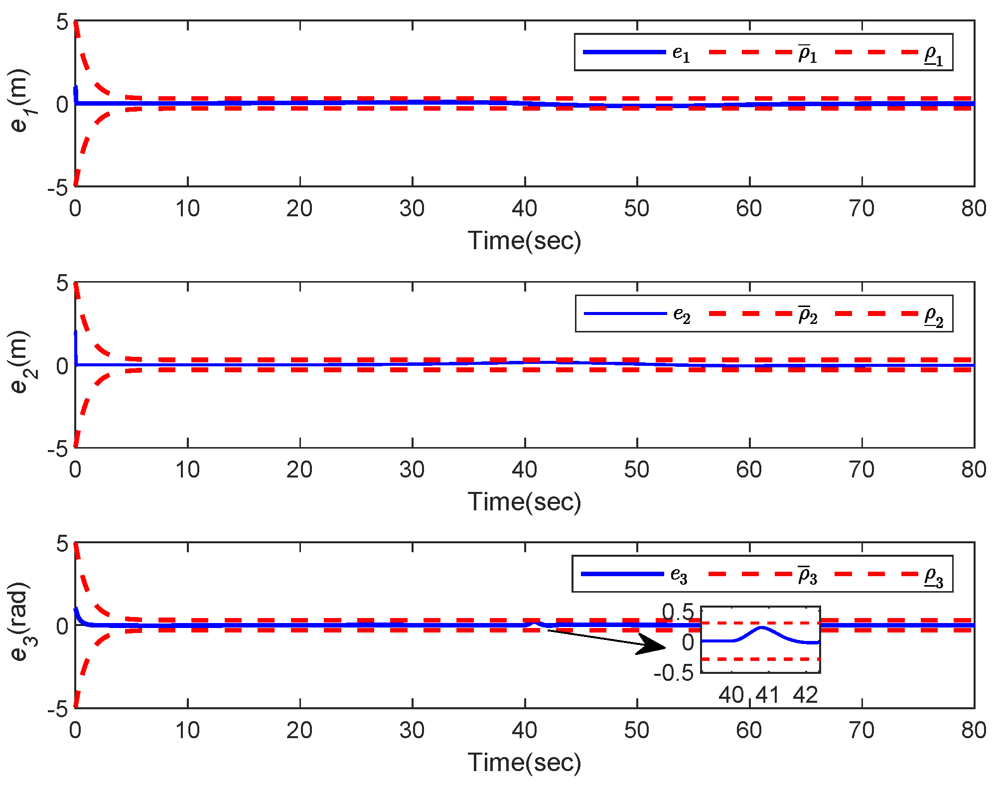
The closed-loop control system is semi-globally stable, i.e., all signals are bounded. The tracking error converges to the origin within the predefined performance (9) at a settling time.

(2)

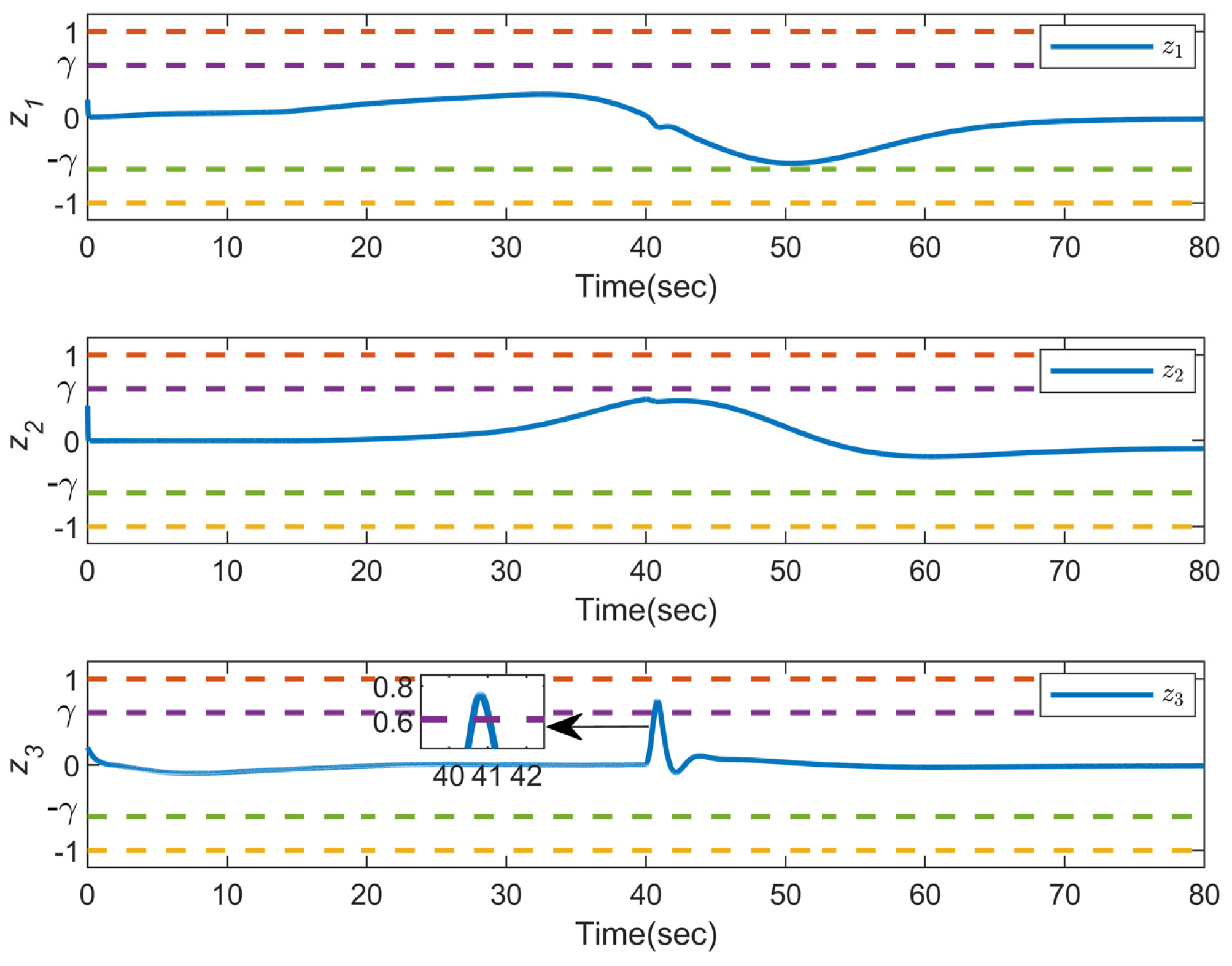
The transformed tracking error provided by the error transformation (11) satisfies

$$|z_i|<\gamma <1,i=1,2,3.$$

(27)

with

$$\begin{array}{cc}\hfill \gamma & =\sqrt{1-{\mathrm{e}}^{-\mu }},\hfill \\ \hfill \mu & =\sum _{i=1}^{3}ln{\displaystyle \frac{1}{1-z_i^2\left(0\right)}}+{\lambda }_{max}\left(M{R}^{-1}\left(0\right)\right){\parallel s\left(0\right)\parallel }^2,\hfill \end{array}$$

(28)

where γ denotes a tighter bound for the guaranteed performance, μ is a constant depending on the initial state.

Proof. 

It can be concluded from (26) that if the control parameters are selected to satisfy $k_1,k_2,k_d>0$, then ${\dot{V}}_2\le 0$. It can be further obtained that

$$\begin{array}{cc}\hfill {\dot{V}}_2\le & -{\lambda }_{min}\left(k_1\right)\sum _{i=1}^{3}ln{\displaystyle \frac{1}{1-z_i^2}}-k_2{\parallel s\parallel }^2-\sum _{i=1}^3{k}_d\left|s_i\right|.\hfill \end{array}$$

(29)

Let ${\zeta }_n=min\{2{\lambda }_{min}\left(k_1\right),2k_2/{\lambda }_{max}\left(\overline{M}\left(\eta \right)\right\}$, we have

$${\dot{V}}_2\le -{\zeta }_n{V}_2.$$

(30)

Integrating (30) from 0 to t yields

$$V_2\left(t\right)\le V_2\left(0\right){\mathrm{e}}^{-{\zeta }_{n}t}\le V_2\left(0\right).$$

(31)

It can be concluded from the above inequality that $ln(1/1-z_i^2)$ and s are bounded. Therefore, $z_i$ remains in $z_i\in (-1,1)$, and all signals in the closed-loop control system are bounded. Proposition 1 implies that tracking error $e_i$ can converge within the predefined performance.

Furthermore, according to (23), it follows that

$$V_2\left(0\right)\le \frac{1}{2}\sum _{i=1}^{3}ln{\displaystyle \frac{1}{1-z_i^2\left(0\right)}}+{\lambda }_{max}\left(M{R}^{-1}\left(0\right)\right){\parallel s\left(0\right)\parallel }^2.$$

(32)

Then, a tighter bound for $z_i$ can be computed by (32), i.e., $z_i<\gamma =\sqrt{1-{\mathrm{e}}^{-\mu }}$, and it is clear that $\gamma <1$ is valid. □

Remark 2. 

To ensure that the tracking errors are kept within the predefined bound, a tighter monitoring bound is required. Through (11), the initial bound for e is transformed to a constant bound for z, so that the monitoring bound for $z_i$ can also be set to a smaller constant. Compared with [44], the complex residual calculations are avoided. Different from the time-varying monitoring bound given in [45], we propose a more concise bound for subsequent fault detection. This simplified approach can make it easier to implement and analyze fault detection and monitoring strategies.

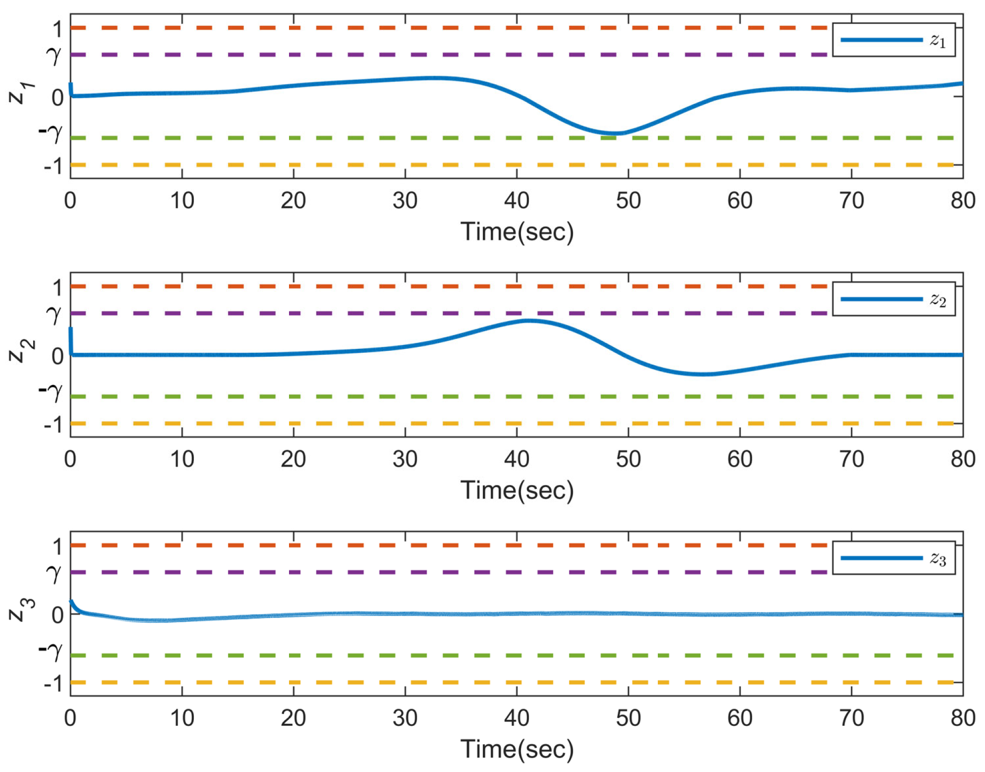
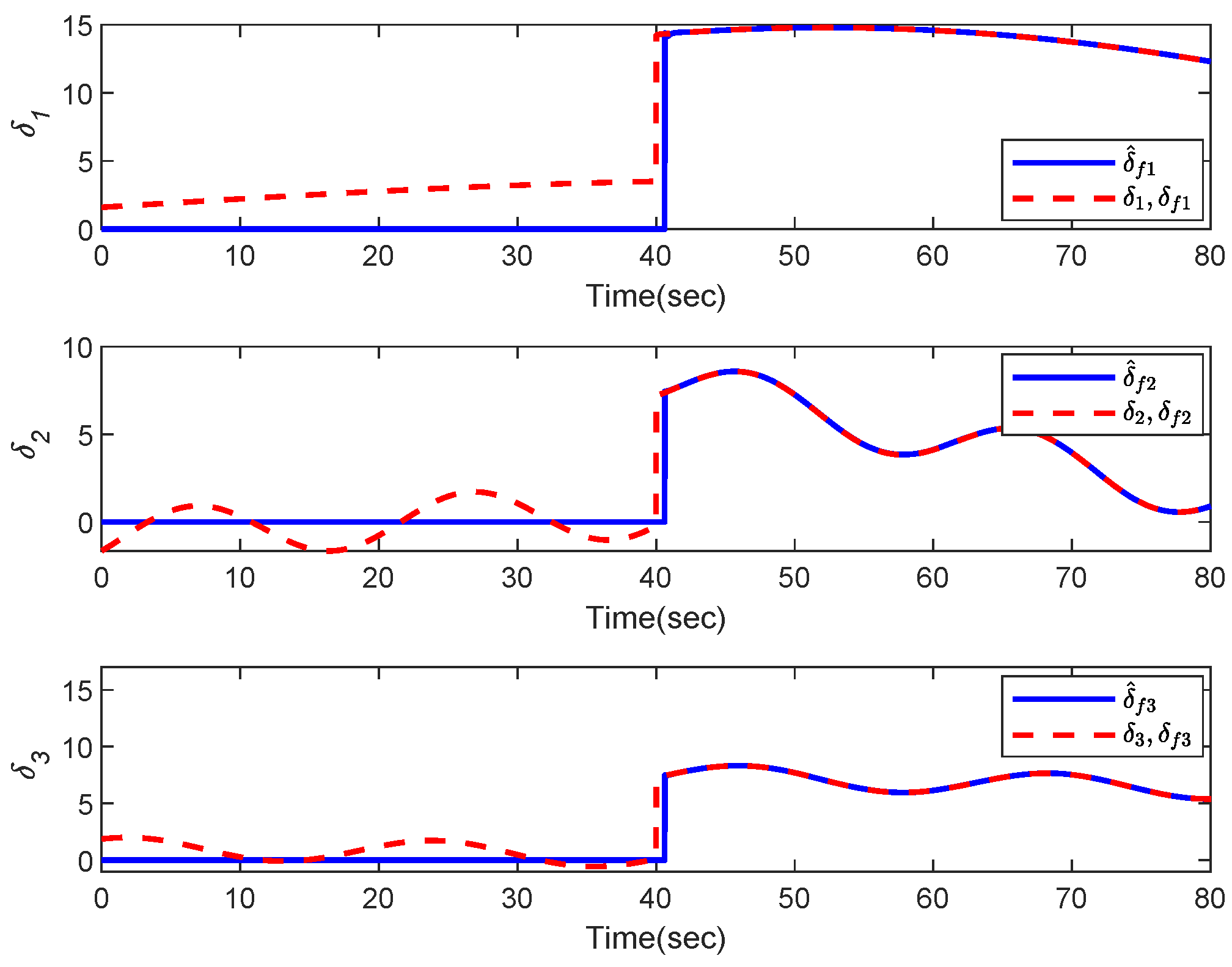
3.2. Fault Detection and Reconfigured Controller Design

In Section 3.1, the nominal controller is presented for the ASV under fault-free condition, and the uncertainty is assumed to be bounded within a known region. However, it is crucial to consider the possibility of faults occurring at any time, denoted as $T_f$. Based on the designed nominal controller, monitoring functions are given to detect the component faults, and a reconfigured controller with a fault estimator are presented.

Theorem 1 indicates that when the fault occurs, the condition given in (27) is violated first before the predefined performance (9) is broken. As a result, by utilizing the tighter bounds presented in (27), we can derive the monitoring functions and identify the precise instant at which the fault is detected as

$$T_d:=inf\{t:|z_i|>\gamma ,i=1,2,3\}.$$

(33)

Once the fault is detected, fault estimation and compensation must be completed as quickly as possible to restore performance.

To guarantee the efficiency of fault estimation and performance restoration, a finite-time fault estimator is presented first. Define new state variables ${\xi }_1=\eta$ and ${\xi }_2=\dot{\eta }$, then the faulty ASV (4) can be described by the following equivalent dynamics:

$$\left\{\begin{array}{c}\begin{array}{cc}\hfill {\dot{\xi }}_1& ={\xi }_2,\hfill \\ \hfill {\dot{\xi }}_2& =-{\kappa }_1\underline{M}\left({\xi }_1\right){\xi }_2+f({\xi }_1,{\xi }_2)+M\left({\xi }_1\right)\tau +\underline{M}\left({\xi }_1\right){\delta }_f,\hfill \end{array}\end{array}\right.$$

(34)

where ${\kappa }_1\in \mathbb{R}$ is a positive constant to be chosen, $\underline{M}\left({\xi }_1\right)=R{M}^{-1}$, $f({\xi }_1,{\xi }_2)=\dot{R}{R}^{-1}{\xi }_2-R{M}^{-1}((C({\xi }_1,{\xi }_2)+D({\xi }_1,{\xi }_2))R^{-1}-{\kappa }_1){\xi }_2$, ${\delta }_f=f_a+{\tau }_d-d\left(t\right)$. It is noted that the upper bound of $\delta$ is unknown due to the component fault is unpredictable.

To obtain the estimation of ${\delta }_f$, an auxiliary state variable ${\xi }_a\in {\mathbb{R}}^3$ is defined, and its dynamics is given as

$${\dot{\xi }}_a=-{\kappa }_1\underline{M}\left({\xi }_1\right){\xi }_a+f({\xi }_1,{\xi }_2)+\underline{M}\left({\xi }_1\right)\tau .$$

(35)

The difference between state variables of (34) and (35) is denoted by ${\xi }_e={\xi }_2-{\xi }_a$. Then, a modified two-order estimator is designed to precisely estimate the lumped uncertainty including fault as

$$\left\{\begin{array}{c}\begin{array}{cc}\hfill {\widehat{\delta }}_f& ={\kappa }_1{\widehat{\xi }}_e+M{R}^{-1}{\dot{\xi }}_e,\hfill \\ \hfill {\dot{\widehat{\xi }}}_e& =-{\kappa }_2{\widehat{\xi }}_e+{\dot{\xi }}_e+{\kappa }_2{\xi }_e+{\kappa }_3\mathrm{sig}{({\tilde{\xi }}_e)}^{\frac{r_1}{r_2}},\hfill \end{array}\end{array}\right.$$

(36)

where

$$\begin{array}{cc}\hfill \mathrm{sig}{({\tilde{\xi }}_e)}^{\frac{r_1}{r_2}}=& [\mathrm{sgn}({\tilde{\xi }}_{e,1})|{\tilde{\xi }}_{e,1}{|}^{\frac{r_1}{r_2}},\mathrm{sgn}({\tilde{\xi }}_{e,2})|{\tilde{\xi }}_{e,2}{|}^{\frac{r_1}{r_2}},\mathrm{sgn}({\tilde{\xi }}_{e,3})|{\tilde{\xi }}_{e,3}{{|}^{\frac{r_1}{r_2}}]}^T,\hfill \end{array}$$

(37)

${\kappa }_2,{\kappa }_3\in \mathbb{R}$ are positive constants to be chosen, $r_1,r_2\in \mathbb{R}$ are positive odd integers and are selected to satisfy $r_1<r_2$. Define the estimation errors of (36) as ${\tilde{\delta }}_f={\delta }_f-{\widehat{\delta }}_f$ and ${\tilde{\xi }}_e={\xi }_e-{\widehat{\xi }}_e$; the following Lemma is obtained.

Lemma 2. 

Based on the modified two-order estimator designed in (36) for the ASV system (4) without component faults, and Assumptions 1–3 holding. Then, the estimation errors ${\tilde{\delta }}_f$ and ${\tilde{\xi }}_e$ can converge to zero in a finite time.

Proof. 

According to the estimator given in Equation (36), the time derivative of ${\tilde{\xi }}_e$ can be calculated as

$$\begin{array}{cc}\hfill {\dot{\tilde{\xi }}}_e& ={\dot{\xi }}_e+{\kappa }_2{\widehat{\xi }}_e-{\dot{\xi }}_e-{\kappa }_2{\xi }_e-{\kappa }_3\mathrm{sig}{({\tilde{\xi }}_e)}^{\frac{r_1}{r_2}}\hfill \\ \hfill & =-{\kappa }_2{\tilde{\xi }}_e-{\kappa }_3\mathrm{sig}{({\tilde{\xi }}_e)}^{\frac{r_1}{r_2}}.\hfill \end{array}$$

(38)

It can be obtained from (34) and (35) that

$$\begin{array}{c}\hfill {\dot{\xi }}_e=-{\kappa }_1\underline{M}\left({\xi }_1\right){\xi }_e+\underline{M}\left({\xi }_1\right){\delta }_f,\end{array}$$

(39)

and

$$\begin{array}{c}\hfill {\tilde{\delta }}_f={\underline{M}}^{-1}\left({\xi }_1\right){\dot{\xi }}_e+{\kappa }_1{\xi }_e-{\kappa }_1{\widehat{\xi }}_e-M{R}^{-1}{\dot{\xi }}_e={\kappa }_1{\tilde{\xi }}_e.\end{array}$$

(40)

Differentiating (40) with respect to time yields

$${\dot{\tilde{\delta }}}_f={\kappa }_1{\dot{\tilde{\xi }}}_e=-{\kappa }_2{\tilde{\delta }}_f-{\kappa }_3\mathrm{sig}{({\tilde{\delta }}_f)}^{\frac{r_1}{r_2}}.$$

(41)

Consider a Lyapunov function for the estimator given in Equation (36) as $V_d=\frac{1}{2}{\tilde{\delta }}_f^T{\tilde{\delta }}_f$, and the time derivative of $V_d$ is given as

$$\begin{array}{cc}\hfill {\dot{V}}_d& ={\tilde{\delta }}_f^T(-{\kappa }_2{\tilde{\delta }}_f-{\kappa }_3\mathrm{sig}{({\tilde{\delta }}_f)}^{\frac{r_1}{r_2}})\hfill \\ \hfill & \le -{\kappa }_2\parallel {\tilde{\delta }}_f{\parallel }^2-{\kappa }_3{\parallel {\tilde{\delta }}_f\parallel }^{\frac{r_1+r_2}{2r_2}}\hfill \\ \hfill & \le -{\mathsf{\Gamma }}_1{V}_d-{\mathsf{\Gamma }}_2{V}_d^r,\hfill \end{array}$$

(42)

where ${\mathsf{\Gamma }}_1=2{\kappa }_2$, $r=\frac{r_1+r_2}{2r_2}$, ${\mathsf{\Gamma }}_2=2^r{\kappa }_3$. It can be concluded from (40) and (42) that $V_d$ is bounded, and the boundedness of ${\tilde{\delta }}_f$ and ${\tilde{\xi }}_e$ can be ensured. It follows from [49] that the estimation errors converge to zero in a finite time, and the convergence time can be obtained as

$$T_c\le {\displaystyle \frac{1}{{\mathsf{\Gamma }}_1(1-r)}}ln{\displaystyle \frac{{\mathsf{\Gamma }}_1{V}^{1-r}({\tilde{\delta }}_f\left(0\right))+{\mathsf{\Gamma }}_2}{{\mathsf{\Gamma }}_2}}.$$

(43)

 □

Based on Lemma 2, the nominal controller can be reconfigured as

$${\tau }_r=-k_{2}s-g(\eta ,\dot{\eta })-\frac{1}{2}\dot{\overline{M}}\left(\eta \right)\dot{\eta }s+\overline{M}\left(\eta \right)\dot{\alpha }-\Sigma -{\widehat{\delta }}_f,$$

(44)

Similar to the analysis in Theorem 1, let $\tau ={\tau }_r$ and substituting (44) into (24) leads to

$${\dot{V}}_2\le -{\lambda }_{min}\left(k_1\right)\sum _{i=1}^3{\displaystyle \frac{z_i^2}{1-z_i^2}}-{\lambda }_{min}\left(k_2\right)s^{T}s-s^T{\tilde{\delta }}_f.$$

(45)

Theorem 2. 

Consider the ASV system described by (4) subject to component faults, and Assumptions 1–3 hold. Assume the component fault occurs at $t=T_f$ and is detected at $t=T_d$, for $t>T_d$, the proposed controller (44) with the estimator (36) can ensure the following:

(1) 

The closed-loop control system is semi-global stable, i.e., all signals are bounded.

(2) 

The transformed tracking error $z_i,i=1,2,3,$ is kept in in the compact set $(-1,1)$.

(3) 

The tracking error can converge to the origin within the predefined performance (9) at a settling time.

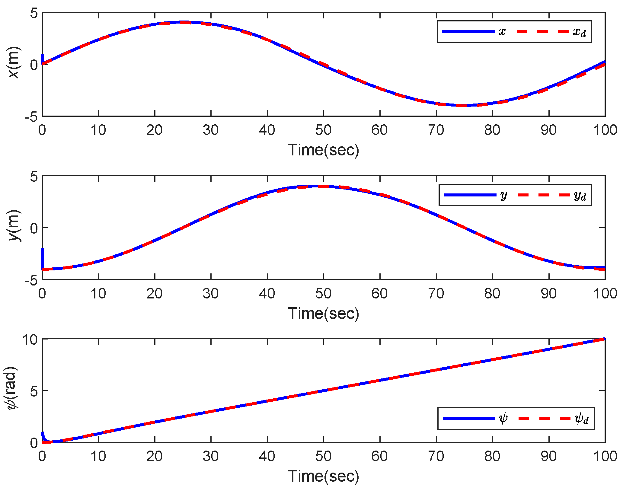
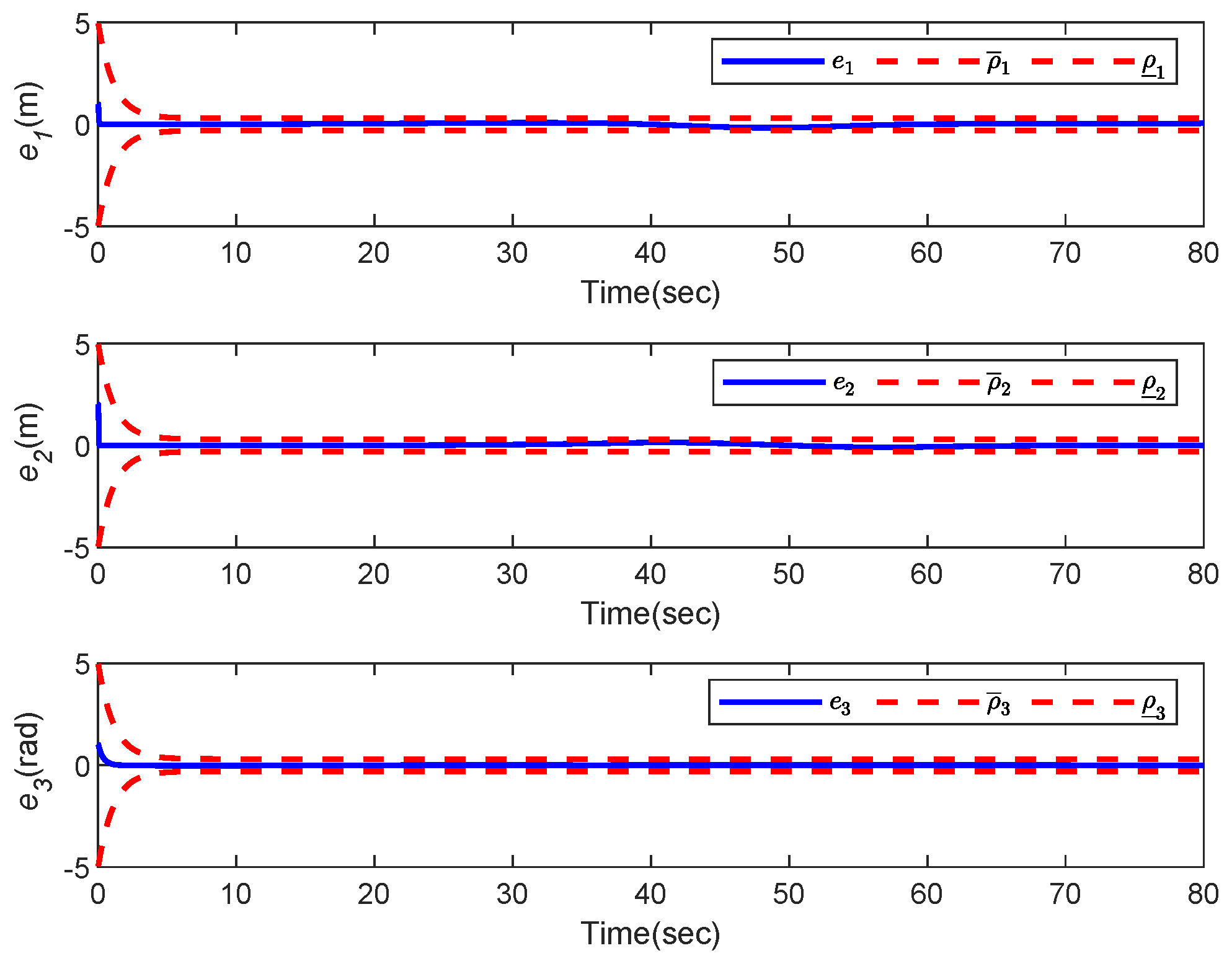
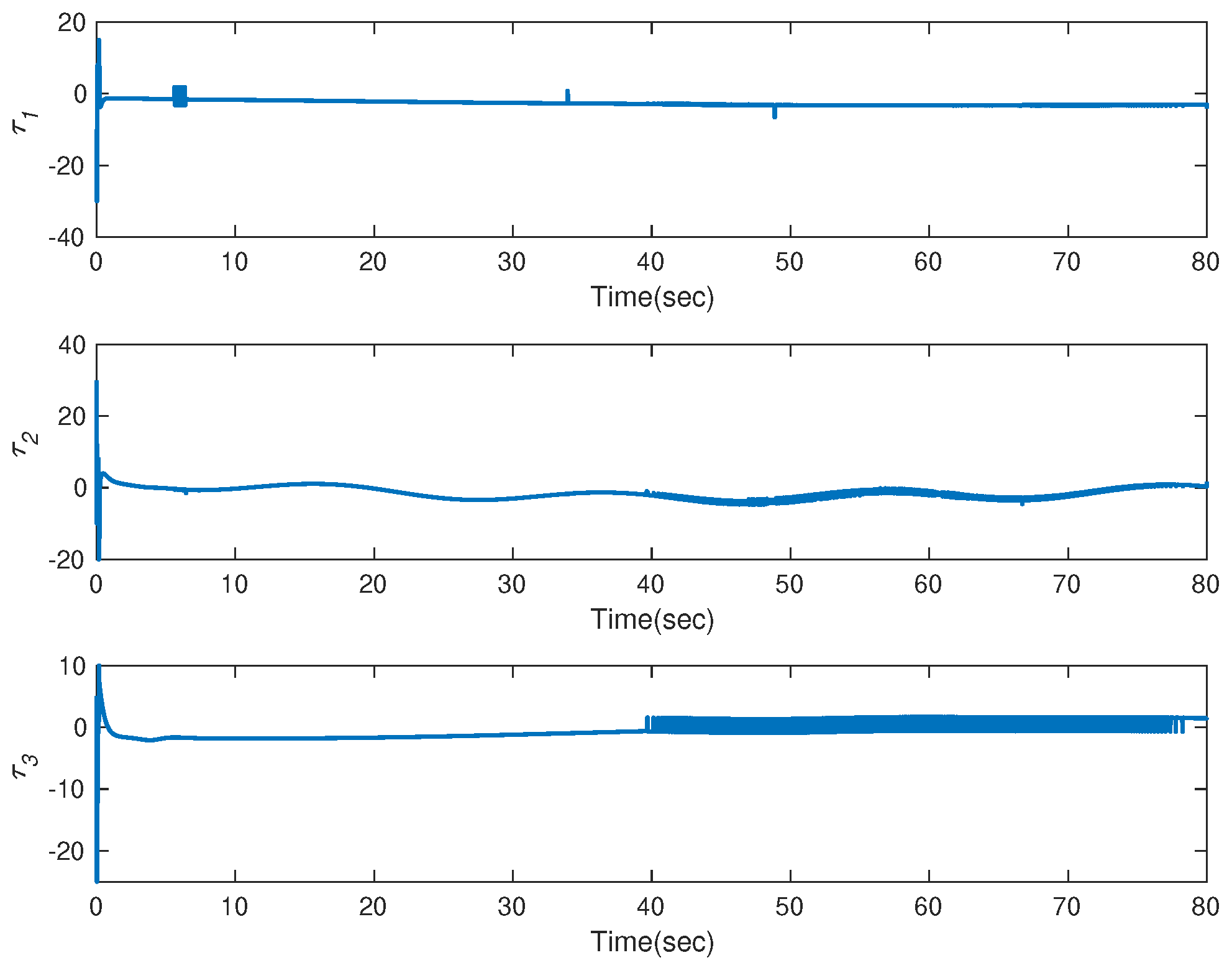
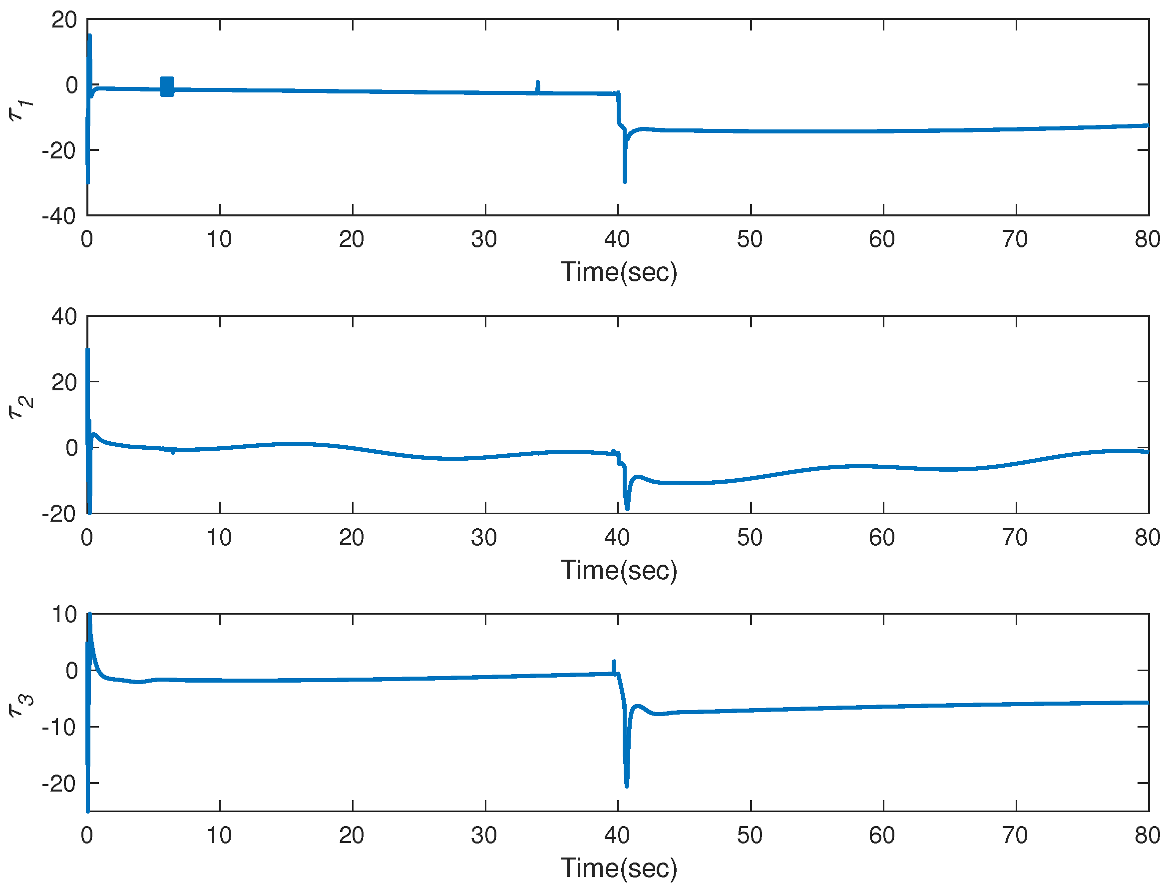
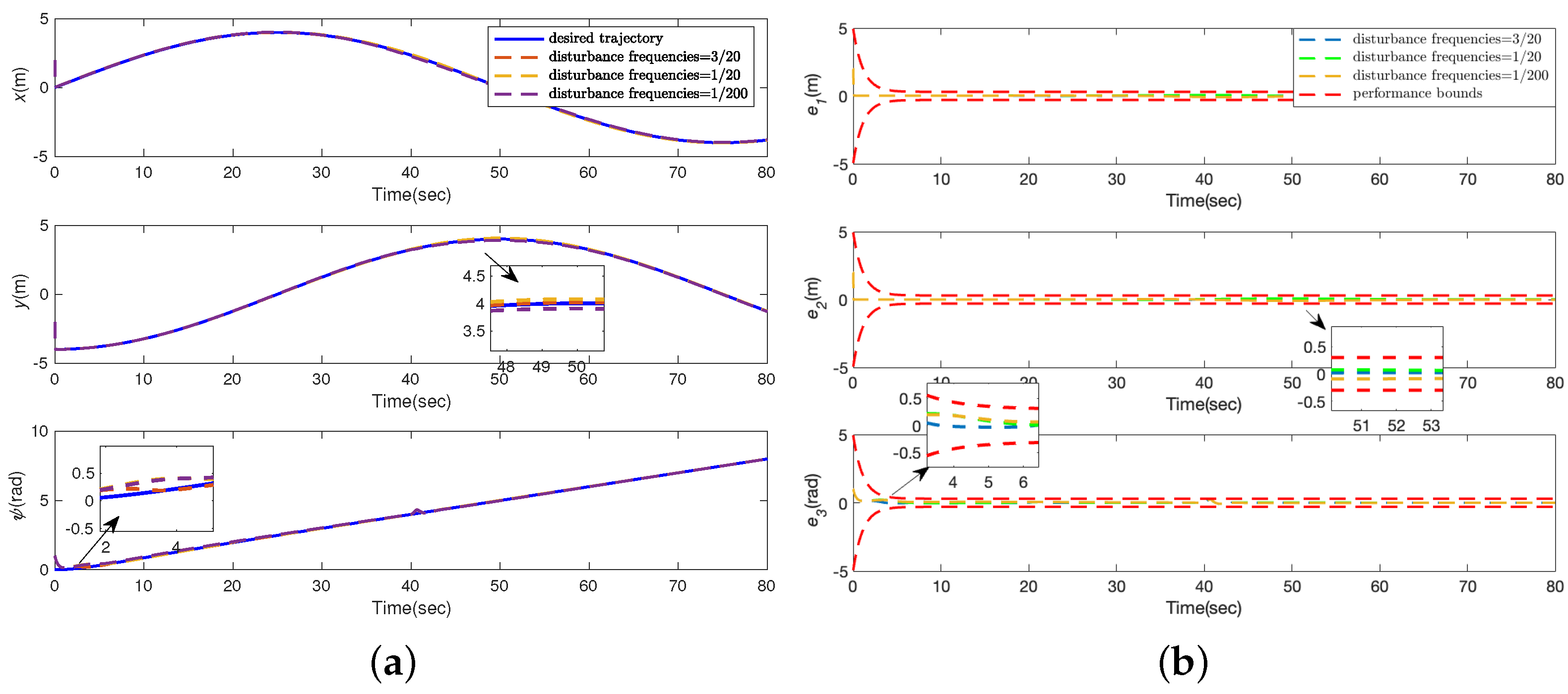
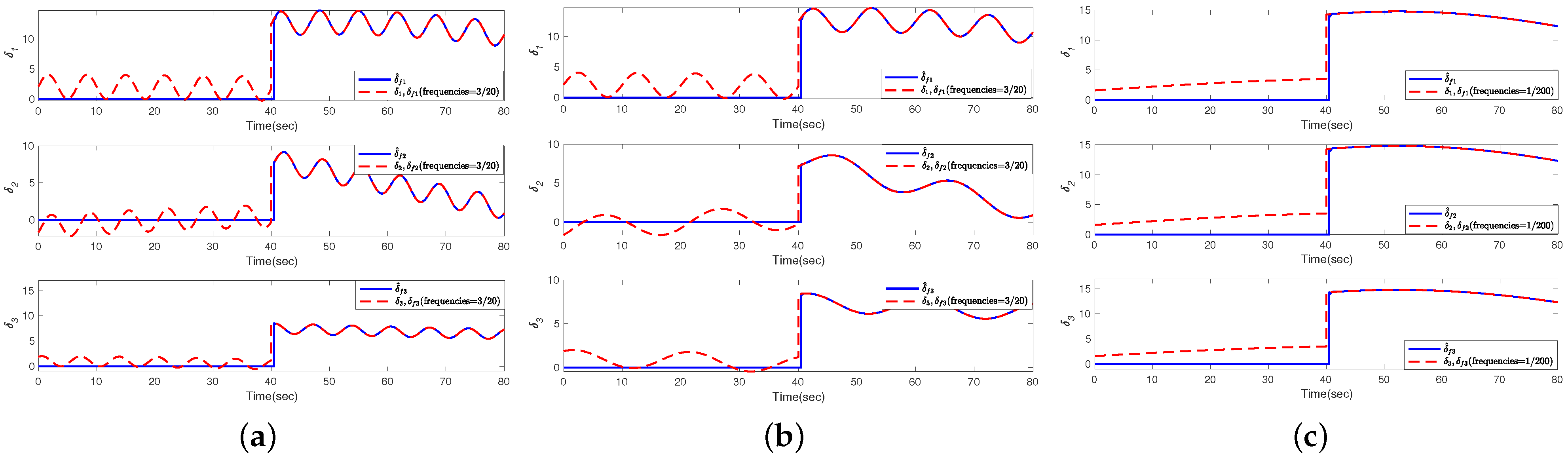
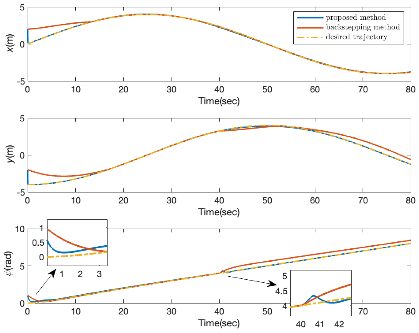
Proof. 

Select the Lyapunov function as

$$V_n=V_2+V_f.$$

(46)

Differentiating $V_n$ and substituting (45) results in

$$\begin{array}{cc}\hfill {\dot{V}}_n\le & -{\lambda }_{min}\left(k_1\right)\sum _{i=1}^3{\displaystyle \frac{z_i^2}{1-z_i^2}}-k_2{s}^{T}s-s^T{\tilde{\delta }}_f+{\dot{V}}_f\hfill \\ \hfill \le & -{\lambda }_{min}\left(k_1\right)\sum _{i=1}^3{\displaystyle \frac{z_i^2}{1-z_i^2}}-\frac{1}{2}{\lambda }_{min}\left((2k_2-I)\right){\parallel s\parallel }^2-({\kappa }_2-\frac{1}{2})\parallel {\tilde{\delta }}_f{\parallel }^2-{\mathsf{\Gamma }}_2{\parallel {\tilde{\delta }}_f\parallel }^{2r}.\hfill \end{array}$$

(47)

If the control parameters are selected to satisfy $k_1>0$, $2k_2-I>0$, ${\kappa }_2>\frac{1}{2}$, it can be obtained that ${\dot{V}}_n\le 0$. Similar to Theorem 1, we can obtain that $z_i$ remains in $z_i\in (-1,1)$, and all signals in the closed-loop control system are bounded. Furthermore, Proposition 1 implies that tracking error $e_i$ converges within the guaranteed performance. □

Remark 3. 

MPC methods have been gradually applied for performance optimization in vehicle trajectory tracking scenarios [50,51,52]. In comparison to the MPC scheme, the advantages of the proposed FTPF + AFTC method are as follows: (1) Fault Recovery Time: the FTPF method imposes strict constraints on both reaction time and convergence range, which cannot be achieved by other methods currently available. (2) Fault Detection: the FTPF method not only ensures tracking performance within an ideal region but also provides a concise bound for designing the monitoring function. (3) Model Mismatch and Measurement Bias: in MPC control, performance can be sensitive to discrepancies between the prediction model and the actual system dynamics, potentially resulting in degraded control performance. If long-term stability is a critical requirement for ASV operations, the FTPF-based AFTC algorithm becomes a preferable choice.

4. Simulation Study

To validate the feasibility of the designed AFTC scheme, a simulation example is carried out on CyberShip II model [53]. The parameters M, $C\left(\nu \right)$, $D\left(\nu \right)$ in (1) are given as

$$\begin{array}{cc}\hfill M& =\left[\begin{array}{ccc}{m}_{11}& 0& 0\\ 0& m_{22}& m_{23}\\ 0& m_{32}& m_{33}\end{array}\right],\hfill \\ \hfill C\left(\nu \right)& =\left[\begin{array}{ccc}0& 0& c_{13}\left(\nu \right)\\ 0& 0& c_{23}\left(\nu \right)\\ -c_{13}\left(\nu \right)& -c_{23}\left(\nu \right)& 0\end{array}\right],\hfill \\ \hfill D\left(\nu \right)& =\left[\begin{array}{ccc}{d}_{11}\left(\nu \right)& 0& 0\\ 0& d_{22}\left(\nu \right)& d_{23}\left(\nu \right)\\ 0& d_{32}\left(\nu \right)& d_{33}\left(\nu \right)\end{array}\right].\hfill \end{array}$$

(48)

where $m_{11}=m_0-X_{\dot{u}}$, $m_{22}=m_0-Y_{\dot{w}}$, $m_{23}=m_0{x}_g-Y_{\dot{r}}$, $m_{32}=m_0{x}_g-N_{\dot{w}}$, $m_{33}=I_z-N_{\dot{r}}$, $c_{13}\left(\nu \right)=-m_{11}w-m_{23}r$, $c_{23}\left(\nu \right)=m_{11}u$, $d_{11}\left(\nu \right)=-X_u-X_{\left|u\right|u}\left|u\right|-X_{uuu}{u}^2$, $d_{22}\left(\nu \right)=-Y_w-Y_{\left|w\right|w}\left|w\right|$, $d_{23}\left(\nu \right)=-Y_r-Y_{\left|w\right|r}\left|w\right|-Y_{\left|r\right|r}\left|r\right|$, $d_{32}\left(\nu \right)=-N_w-N_{\left|w\right|w}\left|w\right|-N_{\left|r\right|w}\left|r\right|$, and $d_{33}\left(\nu \right)=-N_r-N_{\left|w\right|r}\left|w\right|-N_{\left|r\right|r}\left|r\right|$. The system parameters are listed in

Table 1. Main parameters for cybership II.

Factor	Value	Factor	Value	Factor	Value
$m_0$	23.8	$Y_w$	−0.8612	$X_{\dot{u}}$	−2
$I_z$	1.76	$Y_{\left|w\right|w}$	−36.2823	$Y_{\dot{w}}$	−10
$x_g$	0.046	$Y_r$	0.1079	$Y_{\dot{r}}$	0
$X_u$	−0.7225	$N_w$	0.1052	$N_{\dot{w}}$	0
$X_{\left|u\right|u}$	−1.3274	$N_{\left|w\right|w}$	5.0437	$N_{\dot{r}}$	−1
$X_{uuu}$	−5.8664

.

In the simulation example, the control objective is to force the vehicle to track the desired trajectory as ${\eta }_d=[4sin\left(0.02\pi t\right),-4cos\left(0.02\pi t\right),0.1t{(1-{\mathrm{e}}^{-t/5}]}^T$. The initial states of ASV are set as $\eta \left(0\right)={[1,-2,1]}^T$, $\nu \left(0\right)={[0,0,0]}^T$. The parameters of performance function are chosen as ${\rho }_{i0}=4.7,{\rho }_{i{T}_s}=0.3,\iota =1.2,\epsilon =0.3$, $i=1,2,3$, and the settling time can be calculated by (6) as $T_s=4.4190s$. For simplicity, the lumped uncertainty $\delta$ is described in a general term as time-varying forces/moment:

$$\delta =\left\{\begin{array}{c}1.6+2sin\left(0.01\pi t\right)\\ -0.9+1.5sin(0.1\pi t-\pi /6)+1.5sin\left(0.01\pi t\right)\\ sin(0.09\pi t+\pi /3)+cos\left(0.01\pi t\right)\end{array}\right\}.$$

(49)

To verify the fault-tolerant ability of the proposed AFTC scheme, the component faults are intentionally introduced into the ASV control system at a specific time $t=T_f=40 \mathrm{s}$ and $f_a={[6.2+5sin(0.01\pi t-10),5.4+5cos(0.01\pi t-10),7.2+0.3{\mathrm{e}}^{-0.2t}]}^T$. The control system’s response to these faults can be analyzed and assessed to determine the effectiveness of the fault-tolerant control strategy. The control gains are selected as $k_1=\mathrm{diag}(23,28,2)$, $k_2=\mathrm{diag}(1.95,1.7,0.5)$, $k_d=3.5$. According to the initial states, we can calculate that $\gamma =0.6075$. The controller switches from nominal controller to reconfigured controller when $|z_i|>\gamma$ at $t=T_d$. The estimator gains are selected as ${\kappa }_1=0.001$, ${\kappa }_2=0.9$, ${\kappa }_3=15$, $r_1=99$, $r_2=101$.

4.1. Fault-Tolerant Ability Verification

To illustrate the effectiveness of the proposed nominal controller and the reconfigured controller, two experiments are conducted under fault-free and component fault conditions. In the first experiment, the fault-free condition is considered, where no component faults are present in the system. This experiment aims to demonstrate the performance of the control system under a nominal controller when there are no faults affecting the system’s behavior. In the second experiment, the component fault condition is considered. Component faults are intentionally introduced into the system at a specific time, as mentioned earlier. This experiment aims to evaluate the performance of the control system in the presence of component faults. The control system switches from the nominal controller to the reconfigured controller when the fault detection threshold is exceeded. By comparing the results of these two experiments, the effectiveness of both the nominal controller and the reconfigured controller can be evaluated. The control system’s ability to maintain stability, tracking performance, and fault tolerance can be assessed, providing insights into the overall performance of the proposed AFTC scheme.

The simulation results are shown in Figure 2, Figure 3, Figure 4, Figure 5, Figure 6, Figure 7, Figure 8 and Figure 9. Among them, Figure 2, Figure 3 and Figure 4 are the results of fault-free experiment and Figure 6, Figure 7, Figure 8 and Figure 9 are the results of component fault experiment. It can be observed from Figure 2, Figure 3 and Figure 4 that the ASV can follow the given trajectories within the designed nominal controller, and the predefined performance bounds are guaranteed. The trajectories of the ASV closely track the desired reference trajectories in Figure 2, indicating accurate tracking performance. The predefined performance bounds are observed to be satisfied in Figure 3. This ensures that the system operates within the desired performance criteria. The trajectories of transformed error are given in Figure 4, and it is obvious that the transformed errors are kept within the given sets. The control inputs are given in Figure 5.

In Figure 6, Figure 7, Figure 8 and Figure 9, the detection results and the control performance under controller reconfiguration are depicted, which illustrates the system’s behavior during the occurrence of component faults. Figure 6 depicts the curves of desired and actual trajectories of the ASV. The tracking errors and their constraints are illustrated in Figure 7, which reveals that the predefined performance is guaranteed at all times. Although there may be some variation in system performance when the fault occurs, it can be quickly recovered. Figure 8 focuses on the response of the transformed error. As seen from Figure 8, when the component fault occurs at $t=T_f=40\mathrm{s}$, the transformed error z reacts to the fault faster than the tracking error e in Figure 7. This behavior indicates that the fault is detected and reflected in the transformed error before affecting the tracking performance. After the effect of component faults on ASV exceeds the detection threshold, the FE module provides an effective detection signal at $t=T_d=40.8\mathrm{s}$. From Figure 9 we can see that the estimator is activated at $t=T_d$, indicating that the controller reconfiguration has been achieved, and the faults are well estimated. The control inputs are given in Figure 10. These figures demonstrate the system’s response to component faults, the activation of the fault detection module, and the successful transition to the reconfigured controller.

4.2. Robustness Verification

In this subsection, the lumped uncertainties are reset to three distinct frequencies in order to assess the robustness of the controller against various frequency perturbations. The frequencies used for testing are as follows:

$$\left(1\right)\delta =\left\{\begin{array}{c}1.6+2sin\left(0.3\pi t\right)+0.5cos\left(0.01\pi t\right)\\ -0.9+1.5sin(0.3\pi t-\pi /6)+1.5sin\left(0.01\pi t\right)\\ sin(0.3\pi t+\pi /3)+cos\left(0.01\pi t\right)\end{array}\right\}.$$

$$\left(2\right)\delta =\left\{\begin{array}{c}1.6+2sin\left(0.2\pi t\right)+0.5cos\left(0.01\pi t\right)\\ -0.9+1.5sin(0.1\pi t-\pi /6)+1.5sin\left(0.01\pi t\right)\\ sin(0.1\pi t+\pi /3)+cos\left(0.01\pi t\right)\end{array}\right\}.$$

$$\left(3\right)\delta =\left\{\begin{array}{c}1.6+2sin\left(0.01\pi t\right)\\ -0.9+1.5sin(0.1\pi t-\pi /6)+1.5sin\left(0.01\pi t\right)\\ sin(0.01\pi t+\pi /3)+cos\left(0.01\pi t\right)\end{array}\right\}.$$

The above formula is observed to provide a broader frequency range of disturbance. The simulation results are depicted in Figure 11 and Figure 12. It can be inferred from Figure 11 that disturbances at different frequencies do not significantly impact the control performance, demonstrating the robustness of the method against interference. Figure 12 displays the estimation results of the estimator at various frequencies.

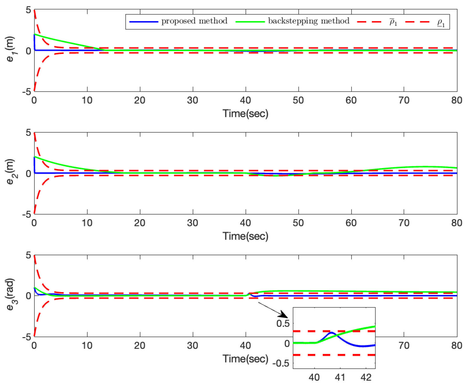
4.3. Advantages Highlight

In order to present a comprehensive assessment of the designed control strategy and demonstrate its superiority, additional numerical simulations were conducted in this subsection. Specifically, we performed a performance comparison between the designed control strategy and a classical backstepping control schemes used in [54]. For the backstepping method, the control input can be provide as follows:

$${\tau }_b=M{R}^{-1}(-k_{b1}s-R{M}^{-1}g(\eta ,\dot{\eta })-\dot{\alpha }-\mathsf{\Phi })$$

(50)

where s is defined as the proposed controller, and $\alpha =-k_{b2}e+{\dot{\eta }}_d$. The remain equations are the same as the proposed controller. It is important to note that the proposed fault detection algorithm, being based on the FTPF, cannot be included in the comparison method. The simulation results of both controllers under fault conditions are presented in Figure 13 and Figure 14. The simulation results for both controllers under fault conditions are depicted in Figure 13 and Figure 14. As illustrated in Figure 13, the proposed controller exhibits a noticeably faster convergence rate compared to the backstepping controller. Furthermore, when component faults occur, the proposed ATFC scheme demonstrates superior fault tolerance, ensuring system stability. In Figure 14, the evolution of the tracking errors is presented, while the backstepping controller can partially guarantee the stability of the ASV, it is evident that without the FTPF, the tracking error cannot be maintained within a predefined range. Overall, these simulation results showcase the capability of the proposed controller to achieve satisfactory tracking performance while ensuring that all outputs remain within their specified ranges.

5. Conclusions

In this paper, a novel AFTC scheme has been investigated to solve the predefined tracking performance problem of ASV with component faults. The integrated AFTC framework has been proposed to accomplish fault detection, fault estimation, and control reconfiguration autonomously. By introducing the error transformation and the Barrier Lyapunov function, a nominal controller was proposed to maintain the control performance under the normal fault-free condition. Within the guaranteed performance, a monitoring function has been designed to supervise the tracking behaviors and report the occurrence of faults. With the signal of the monitoring function, the reconfigured controller was activated, and the lumped uncertainty including fault was estimated precisely by a modified finite-time estimator. Finally, the effectiveness of the proposed AFTC controller has been verified by three aspects: fault-tolerant ability, robustness, and highlighted advantages. The simulation results demonstrate the system’s fast response to faults, the activation of the fault detection module, and the successful transition to the reconfigured controller. The comparative simulations further show the superiority of the proposed method.

References

1. Liu, Z.; Zhang, Y.; Yu, X.; Yuan, C. Unmanned surface vehicles: An overview of developments and challenges. Annu. Rev. Control 2016, 41, 71–93. [Google Scholar] [CrossRef]
2. Shi, Y.; Shen, C.; Fang, H.; Li, H. Advanced Control in Marine Mechatronic Systems: A Survey. IEEE/ASME Trans. Mechatron. 2017, 22, 1121–1131. [Google Scholar] [CrossRef]
3. Ren, Y.; Zhang, L.; Ying, Y.; Li, S.; Tang, Y. Model-Parameter-Free Prescribed Time Trajectory Tracking Control for Under-Actuated Unmanned Surface Vehicles with Saturation Constraints and External Disturbances. J. Mar. Sci. Eng. 2023, 11, 1717. [Google Scholar] [CrossRef]
4. Li, Z.; Xu, W.; Yu, J.; Wang, C.; Cui, G. Finite-Time Adaptive Heading Tracking Control for Surface Vehicles with Full State Constraints. IEEE Trans. Circuits Syst. II Express Briefs 2022, 69, 1134–1138. [Google Scholar] [CrossRef]
5. Zheng, Z.; Huang, Y.; Xie, L.; Zhu, B. Adaptive Trajectory Tracking Control of a Fully Actuated Surface Vessel with Asymmetrically Constrained Input and Output. IEEE Trans. Control Syst. Technol. 2018, 26, 1851–1859. [Google Scholar] [CrossRef]
6. Yan, X.; Jiang, D.; Miao, R.; Li, Y. Formation Control and Obstacle Avoidance Algorithm of a Multi-USV System Based on Virtual Structure and Artificial Potential Field. J. Mar. Sci. Eng. 2021, 9, 161. [Google Scholar] [CrossRef]
7. Gao, S.; Peng, Z.; Liu, L.; Wang, D.; Han, Q.L. Fixed-Time Resilient Edge-Triggered Estimation and Control of Surface Vehicles for Cooperative Target Tracking under Attacks. IEEE Trans. Intell. Veh. 2023, 8, 547–556. [Google Scholar] [CrossRef]
8. Zhou, Z.; Li, M.; Hao, Y. A Novel Region-Construction Method for Multi-USV Cooperative Target Allocation in Air-Ocean Integrated Environments. J. Mar. Sci. Eng. 2023, 11, 1369. [Google Scholar] [CrossRef]
9. Gu, N.; Wang, D.; Peng, Z.; Wang, J.; Han, Q.L. Disturbance observers and extended state observers for marine vehicles: A survey. Control Eng. Pract. 2022, 123, 105158. [Google Scholar] [CrossRef]
10. Zhang, G.; Chu, S.; Huang, J.; Zhang, W. Robust adaptive fault-tolerant control for unmanned surface vehicle via the multiplied event-triggered mechanism. Ocean Eng. 2022, 249, 110755. [Google Scholar] [CrossRef]
11. Liu, Z.; Ge, X.; Han, Q.; Wang, Y.; Zhang, X. Secure Cooperative Path Following of Autonomous Surface Vehicles under Cyber and Physical Attacks. IEEE Trans. Intell. Veh. 2023, 8, 3680–3691. [Google Scholar] [CrossRef]
12. Wu, W.; Tong, S. Fixed-time formation fault tolerant control for unmanned surface vehicle systems with intermittent actuator faults. Ocean Eng. 2023, 281, 114813. [Google Scholar] [CrossRef]
13. Liu, C.; Zhao, X.; Wang, X.; Ren, X. Adaptive fault identification and reconfigurable fault-tolerant control for unmanned surface vehicle with actuator magnitude and rate faults. Int. J. Robust Nonlinear Control 2023, 33, 5463–5483. [Google Scholar] [CrossRef]
14. Liu, L.; Wang, D.; Peng, Z. State recovery and disturbance estimation of unmanned surface vehicles based on nonlinear extended state observers. Ocean Eng. 2019, 171, 625–632. [Google Scholar] [CrossRef]
15. Jiang, J.; Yu, X. Fault-tolerant control systems: A comparative study between active and passive approaches. Annu. Rev. Control 2012, 36, 60–72. [Google Scholar] [CrossRef]
16. Wang, X.; Wang, Q.; Sun, C. Prescribed Performance Fault-Tolerant Control for Uncertain Nonlinear MIMO System Using Actor–Critic Learning Structure. IEEE Trans. Neural Netw. Learn. Syst. 2022, 33, 4479–4490. [Google Scholar] [CrossRef]
17. Shao, X.; Hu, Q.; Shi, Y.; Jiang, B. Fault-Tolerant Prescribed Performance Attitude Tracking Control for Spacecraft under Input Saturation. IEEE Trans. Control Syst. Technol. 2020, 28, 574–582. [Google Scholar] [CrossRef]
18. Yang, W.; Yu, W.; Zheng, W.X. Fault-Tolerant Adaptive Fuzzy Tracking Control for Nonaffine Fractional-Order Full-State-Constrained MISO Systems with Actuator Failures. IEEE Trans. Cybern. 2022, 52, 8439–8452. [Google Scholar] [CrossRef]
19. Saeed Nasrolahi, S.; Abdollahi, F.; Rezaee, H. Decentralized active sensor fault tolerance in attitude control of satellite formation flying. Int. J. Robust Nonlinear Control 2020, 30, 8340–8361. [Google Scholar] [CrossRef]
20. Cai, M.; He, X.; Zhou, D. An active fault tolerance framework for uncertain nonlinear high-order fully-actuated systems. Automatica 2023, 152, 110969. [Google Scholar] [CrossRef]
21. Hu, H.; Wang, B.; Cheng, Z.; Liu, L.; Wang, Y.; Luo, X. A novel active fault-tolerant control for spacecrafts with full state constraints and input saturation. Aerosp. Sci. Technol. 2021, 108, 106368. [Google Scholar] [CrossRef]
22. Hwang, I.; Kim, S.; Kim, Y.; Seah, C.E. A Survey of Fault Detection, Isolation, and Reconfiguration Methods. IEEE Trans. Control Syst. Technol. 2010, 18, 636–653. [Google Scholar] [CrossRef]
23. Qiu, A.; Al-Dabbagh, A.W.; Chen, T. A Tradeoff Approach for Optimal Event-Triggered Fault Detection. IEEE Trans. Ind. Electron. 2019, 66, 2111–2121. [Google Scholar] [CrossRef]
24. Shahriari-kahkeshi, M.; Sheikholeslam, F.; Askari, J. Adaptive fault detection and estimation scheme for a class of uncertain nonlinear systems. Nonlinear Dyn. 2015, 79, 2623–2637. [Google Scholar] [CrossRef]
25. Wang, N.; Lv, S.; Er, M.J.; Chen, W.H. Fast and Accurate Trajectory Tracking Control of an Autonomous Surface Vehicle with Unmodeled Dynamics and Disturbances. IEEE Trans. Intell. Veh. 2016, 1, 230–243. [Google Scholar] [CrossRef]
26. Walker, K.L.; Gabl, R.; Aracri, S.; Cao, Y.; Stokes, A.A.; Kiprakis, A.; Giorgio-Serchi, F. Experimental Validation of Wave Induced Disturbances for Predictive Station Keeping of a Remotely Operated Vehicle. IEEE Robot. Autom. Lett. 2021, 6, 5421–5428. [Google Scholar] [CrossRef]
27. Walker, K.L.; Giorgio-Serchi, F. Disturbance Preview for Non-Linear Model Predictive Trajectory Tracking of Underwater Vehicles in Wave Dominated Environments. In Proceedings of the 2023 IEEE/RSJ International Conference on Intelligent Robots and Systems (IROS), Detroit, MI, USA, 1–5 October 2023; pp. 6169–6176. [Google Scholar] [CrossRef]
28. Zhang, Z.H.; Yang, G.H. Distributed Fault Detection and Isolation for Multiagent Systems: An Interval Observer Approach. IEEE Trans. Syst. Man Cybern. Syst. 2020, 50, 2220–2230. [Google Scholar] [CrossRef]
29. Wang, X. Active Fault Tolerant Control for Unmanned Underwater Vehicle with Sensor Faults. IEEE Trans. Instrum. Meas. 2020, 69, 9485–9495. [Google Scholar] [CrossRef]
30. Rout, R.; Cui, R.; Han, Z. Modified Line-of-Sight Guidance Law with Adaptive Neural Network Control of Underactuated Marine Vehicles with State and Input Constraints. IEEE Trans. Control Syst. Technol. 2020, 28, 1902–1914. [Google Scholar] [CrossRef]
31. Wang, T.; Liu, Y.; Zhang, X. Extended state observer-based fixed-time trajectory tracking control of autonomous surface vessels with uncertainties and output constraints. ISA Trans. 2022, 128, 174–183. [Google Scholar] [CrossRef]
32. Zhang, J.; Yu, S.; Yan, Y. Fixed-time extended state observer-based trajectory tracking and point stabilization control for marine surface vessels with uncertainties and disturbances. Ocean Eng. 2019, 186, 106109. [Google Scholar] [CrossRef]
33. Fu, H.; Yao, W.; Cajo, R.; Zhao, S. Trajectory Tracking Predictive Control for Unmanned Surface Vehicles with Improved Nonlinear Disturbance Observer. J. Mar. Sci. Eng. 2023, 11, 1874. [Google Scholar] [CrossRef]
34. Liu, W.; Ye, H.; Yang, X. Model-Free Adaptive Sliding Mode Control Method for Unmanned Surface Vehicle Course Control. J. Mar. Sci. Eng. 2023, 11, 1904. [Google Scholar] [CrossRef]
35. Bechlioulis, C.P.; Rovithakis, G.A. Adaptive control with guaranteed transient and steady state tracking error bounds for strict feedback systems. Automatica 2009, 45, 532–538. [Google Scholar] [CrossRef]
36. Liu, Y.J.; Zeng, Q.; Tong, S.; Chen, C.P.; Liu, L. Actuator failure compensation-based adaptive control of active suspension systems with prescribed performance. IEEE Trans. Ind. Electron. 2019, 67, 7044–7053. [Google Scholar] [CrossRef]
37. Theodorakopoulos, A.; Rovithakis, G.A. Low-Complexity Prescribed Performance Control of Uncertain MIMO Feedback Linearizable Systems. IEEE Trans. Autom. Control 2016, 61, 1946–1952. [Google Scholar] [CrossRef]
38. Bikas, L.N.; Rovithakis, G.A. Combining Prescribed Tracking Performance and Controller Simplicity for a Class of Uncertain MIMO Nonlinear Systems with Input Quantization. IEEE Trans. Autom. Control 2019, 64, 1228–1235. [Google Scholar] [CrossRef]
39. Wang, H.; Li, M.; Zhang, C.; Shao, X. Event-Based Prescribed Performance Control for Dynamic Positioning Vessels. IEEE Trans. Circuits Syst. II Express Briefs 2021, 68, 2548–2552. [Google Scholar] [CrossRef]
40. Zhang, J.; Chai, T. Singularity-Free Continuous Adaptive Control of Uncertain Underactuated Surface Vessels with Prescribed Performance. IEEE Trans. Syst. Man Cybern. Syst. 2022, 52, 5646–5655. [Google Scholar] [CrossRef]
41. Liu, Y.; Liu, X.; Jing, Y.; Zhang, Z. A Novel Finite-Time Adaptive Fuzzy Tracking Control Scheme for Nonstrict Feedback Systems. IEEE Trans. Fuzzy Syst. 2019, 27, 646–658. [Google Scholar] [CrossRef]
42. Sui, S.; Tong, S. Finite-Time Fuzzy Adaptive PPC for Nonstrict-Feedback Nonlinear MIMO Systems. IEEE Trans. Cybern. 2023, 53, 732–742. [Google Scholar] [CrossRef]
43. Cheng, W.; Zhang, K.; Jiang, B. Fixed-Time Fault-Tolerant Formation Control for a Cooperative Heterogeneous Multiagent System with Prescribed Performance. IEEE Trans. Syst. Man Cybern. Syst. 2023, 53, 462–474. [Google Scholar] [CrossRef]
44. Wang, X. Active Fault Tolerant Control for Unmanned Underwater Vehicle with Actuator Fault and Guaranteed Transient Performance. IEEE Trans. Intell. Veh. 2021, 6, 470–479. [Google Scholar] [CrossRef]
45. Ouyang, H.; Lin, Y. Adaptive Fault-Tolerant Control and Performance Recovery against Actuator Failures with Deferred Actuator Replacement. IEEE Trans. Autom. Control 2021, 66, 3810–3817. [Google Scholar] [CrossRef]
46. Zhang, J.; Yang, G. Supervisory switching-based prescribed performance control of unknown nonlinear systems against actuator failures. Int. J. Robust Nonlinear Control 2020, 30, 2367–2385. [Google Scholar] [CrossRef]
47. Wang, W.; Wen, C. Adaptive actuator failure compensation control of uncertain nonlinear systems with guaranteed transient performance. Automatica 2010, 46, 2082–2091. [Google Scholar] [CrossRef]
48. Tee, K.P.; Ge, S.S.; Tay, E.H. Barrier Lyapunov functions for the control of output-constrained nonlinear systems. Automatica 2009, 45, 918–927. [Google Scholar] [CrossRef]
49. Yu, S.; Yu, X.; Shirinzadeh, B.; Man, Z. Continuous finite-time control for robotic manipulators with terminal sliding mode. Automatica 2005, 41, 1957–1964. [Google Scholar] [CrossRef]
50. Wei, H.; Shi, Y. Mpc-based motion planning and control enables smarter and safer autonomous marine vehicles: Perspectives and a tutorial survey. IEEE/CAA J. Autom. Sin. 2023, 10, 8–24. [Google Scholar] [CrossRef]
51. Guerreiro, B.J.; Silvestre, C.; Cunha, R.; Pascoal, A. Trajectory Tracking Nonlinear Model Predictive Control for Autonomous Surface Craft. IEEE Trans. Control Syst. Technol. 2014, 22, 2160–2175. [Google Scholar] [CrossRef]
52. Cui, Y.; Peng, L.; Li, H. Filtered Probabilistic Model Predictive Control-Based Reinforcement Learning for Unmanned Surface Vehicles. IEEE Trans. Ind. Inform. 2022, 18, 6950–6961. [Google Scholar] [CrossRef]
53. Skjetne, R.; Fossen, T.I.; Kokotović, P.V. Adaptive maneuvering, with experiments, for a model ship in a marine control laboratory. Automatica 2005, 41, 289–298. [Google Scholar] [CrossRef]
54. Ouyang, H.; Lin, Y. Adaptive fault-tolerant control for actuator failures: A switching strategy. Automatica 2017, 81, 87–95. [Google Scholar] [CrossRef]
Figure 1. ASV model with two right-hand coordinate systems.
Jmse 12 00347 g001
Figure 2. Fault−free experiments: trajectories under the nominal controller.
Jmse 12 00347 g002
Figure 3. Fault-free experiments: tracking errors with performance bounds.
Jmse 12 00347 g003
Figure 4. Fault-free experiments: transformed errors and monitoring functions.
Jmse 12 00347 g004
Figure 5. Fault-free experiments: control inputs.
Jmse 12 00347 g005
Figure 6. AFTC experiments: trajectories under the nominal and reconfigured controller.
Jmse 12 00347 g006
Figure 7. AFTC experiments: tracking errors with performance bounds.
Jmse 12 00347 g007
Figure 8. AFTC experiments: transformed errors and monitoring functions.
Jmse 12 00347 g008
Figure 9. AFTC experiments: the lumped uncertainties and their estimations (after T d ).
Jmse 12 00347 g009
Figure 10. AFTC experiments: control inputs.
Jmse 12 00347 g010
Figure 11. Robustness experiments: tracking performance under different frequency disturbance. (a) Trajectory tracking performance. (b) Tracking errors.
Jmse 12 00347 g011
Figure 12. Robustness experiments: uncertainties estimation under different frequency disturbance. (a) Disturbance frequency = 3/20. (b) Disturbance frequency = 1/20. (c) Disturbance frequency = 1/200.
Jmse 12 00347 g012
Figure 13. Comparison experiments: trajectories under the proposed controller and backstepping controller.
Jmse 12 00347 g013
Figure 14. Comparison experiments: tracking errors under the proposed controller and backstepping controller.
Jmse 12 00347 g014