
A Multi-Ship Collision Avoidance Algorithm Using Data-Driven Multi-Agent Deep Reinforcement Learning

Abstract
:1. Introduction
2. Literature Review
3. Multi-Ship Collision Avoidance Decision-Making Algorithm Design
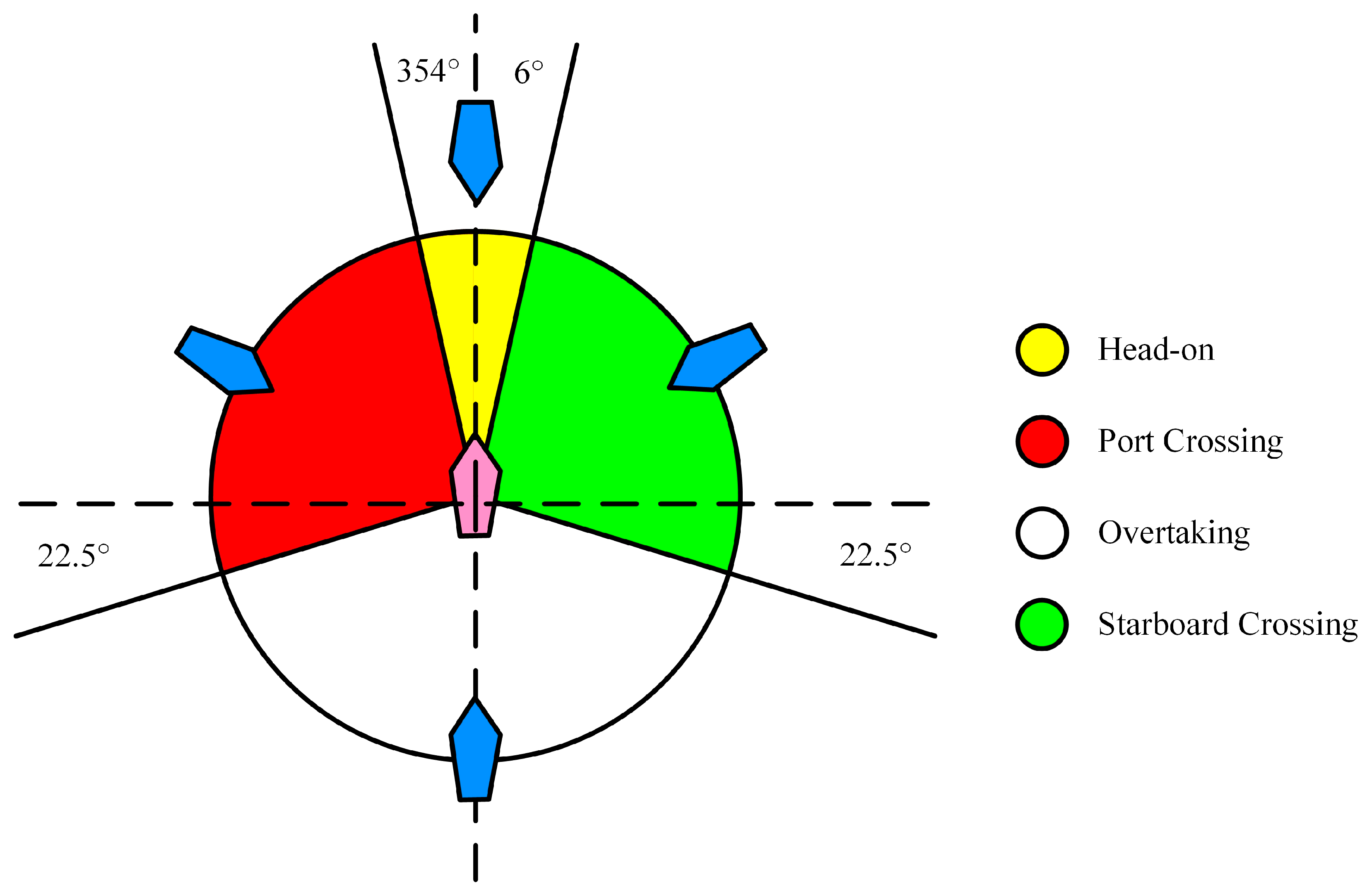
3.1. COLREGs
- Rule 13 (Overtaking): If a vessel is deemed to be overtaking when coming up with another vessel from a direction more than 22.5° above her beam, the situation is considered to be overtaking. Notwithstanding anything contained in the Rules of Part B, Sections I and II, any vessel overtaking any other shall keep out of the way of the vessel being overtaken.
- Rule 14 (Head-on situation): Each ship should turn to the starboard and pass on the port side of the other ship when there is a risk of collision.
- Rule 15 (Crossing situation): If the courses of two vessels cross, the situation is considered as crossing situation; When two power-driven vessels are crossing so as to involve risk of collision, the vessel which has the other on her own starboard side shall keep out of the way and shall, if the circumstances of the case admit, avoid crossing ahead of the other vessel.
3.2. Ship Coordinated and Uncoordinated Behaviors
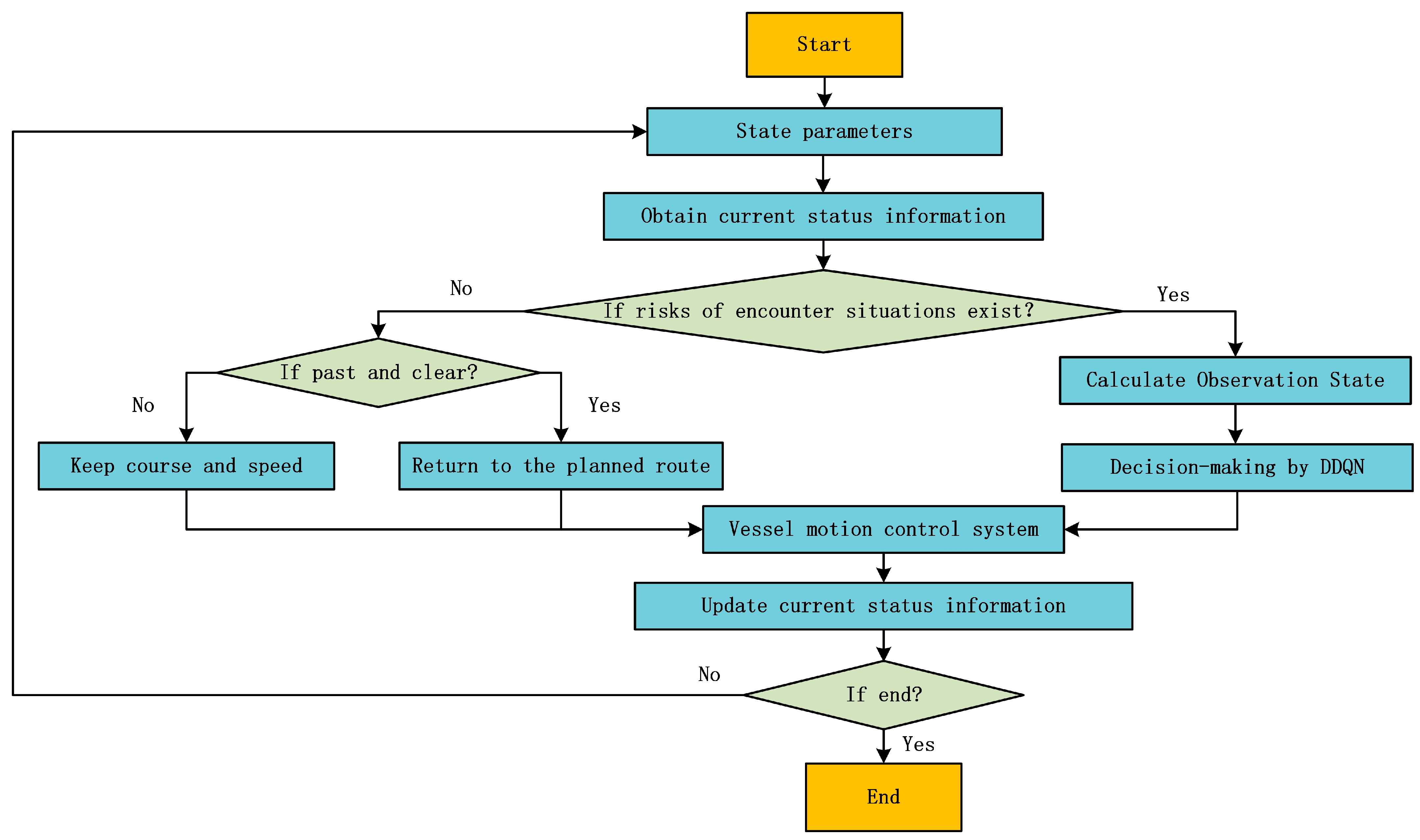
3.3. Flow Chart
3.4. Definition of Ship Collision Avoidance Problem Based on MDP
- is a finite set of environment states; is the current environment state, which mainly includes ships, dynamic obstacles, static obstacles, etc.
- is the set of observed states of the agents; is the observation state obtained by the agent in the environment at the moment .
- is the action space set of the agents; is the action performed by the agent at the moment , generated by the policy function .
- is the state transfer function and is the probability that the state is transferred from to after the agent performs the action at the moment .
- is the reward function; is the reward that the agent receives from the environment at the moment .
- is the decay value for future reward; is the learning rate of the agent.
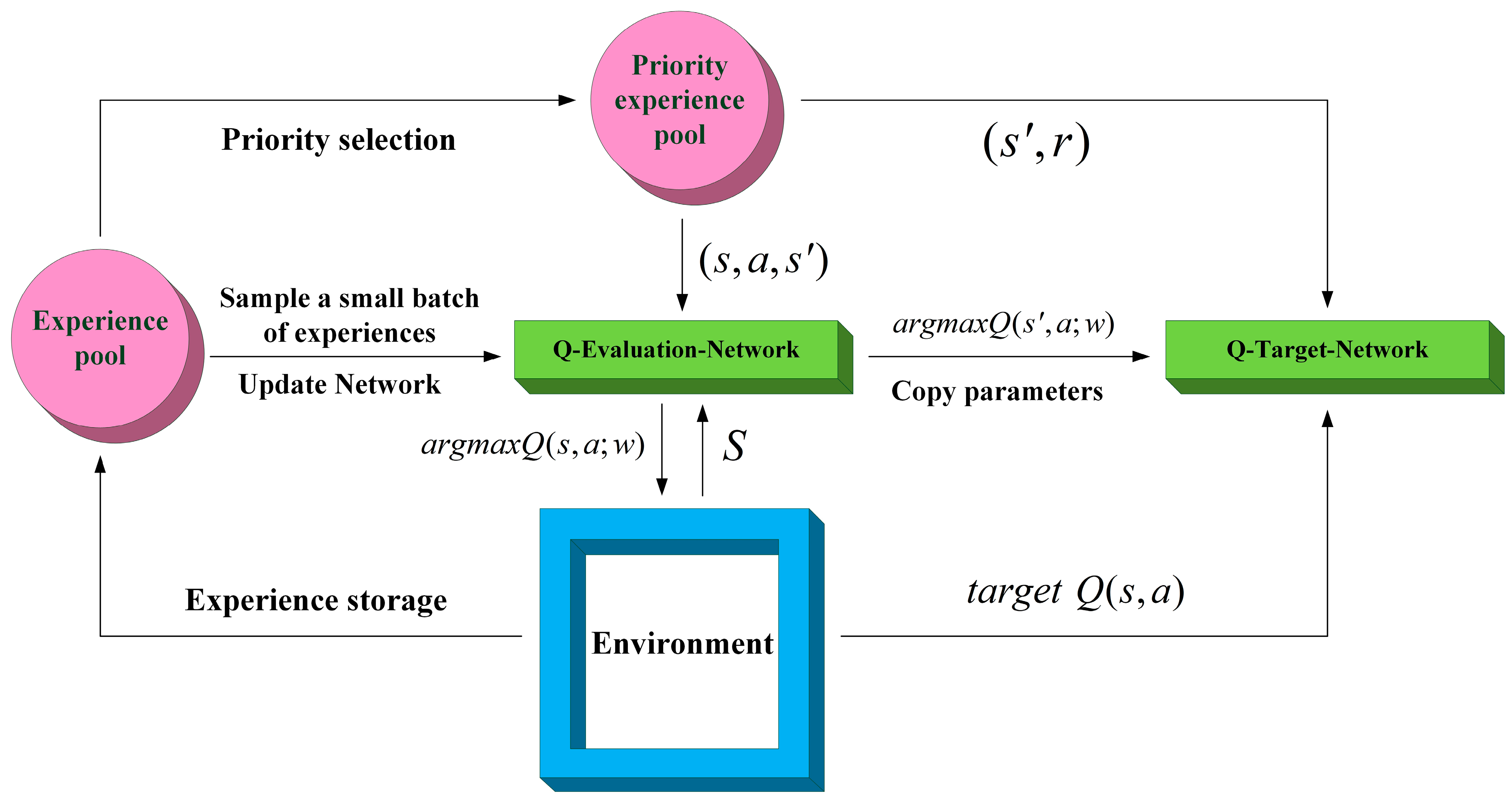
3.5. PER-DDQN
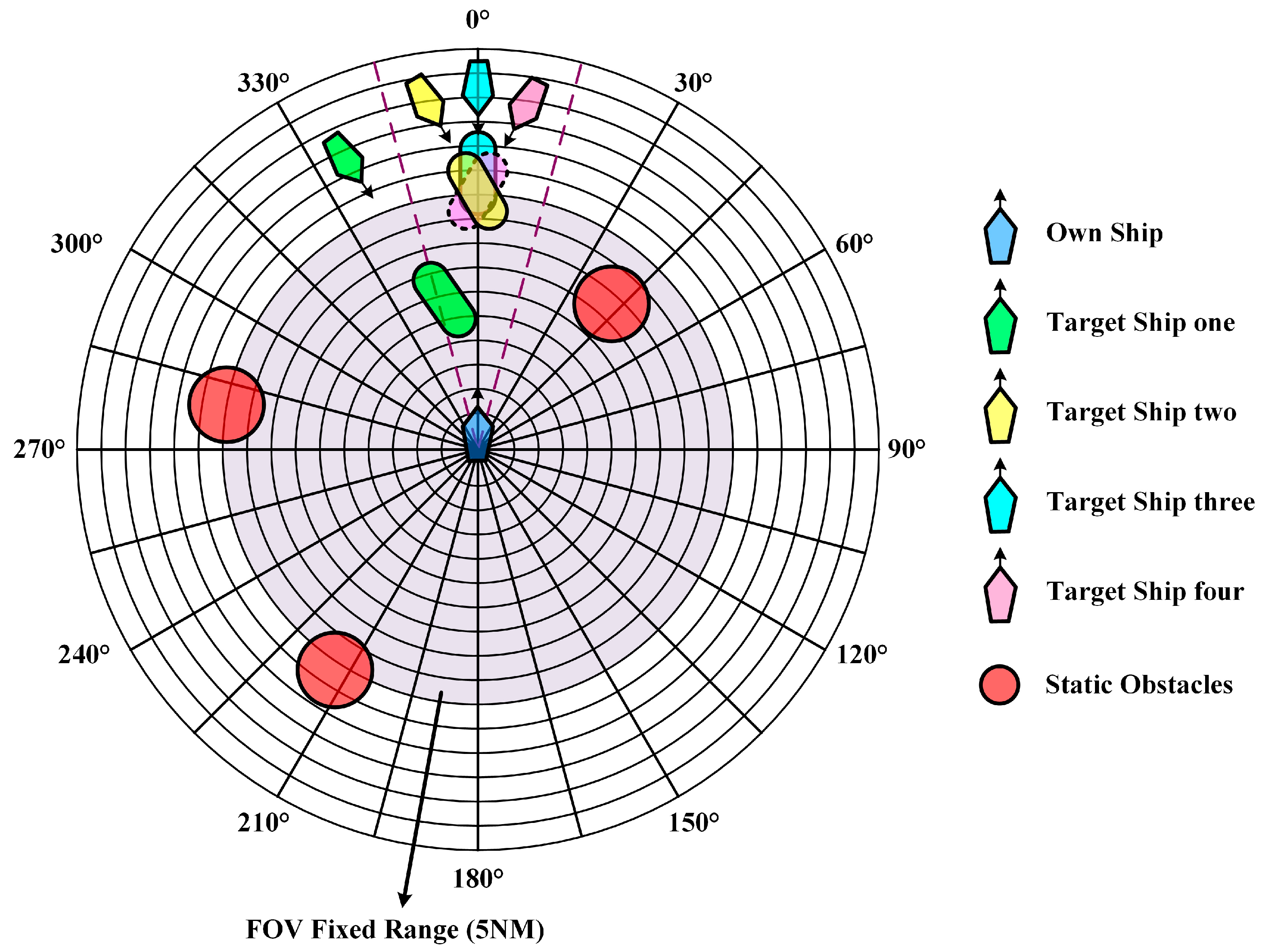
3.6. Observation State
3.7. Action Space
3.8. Reward Function
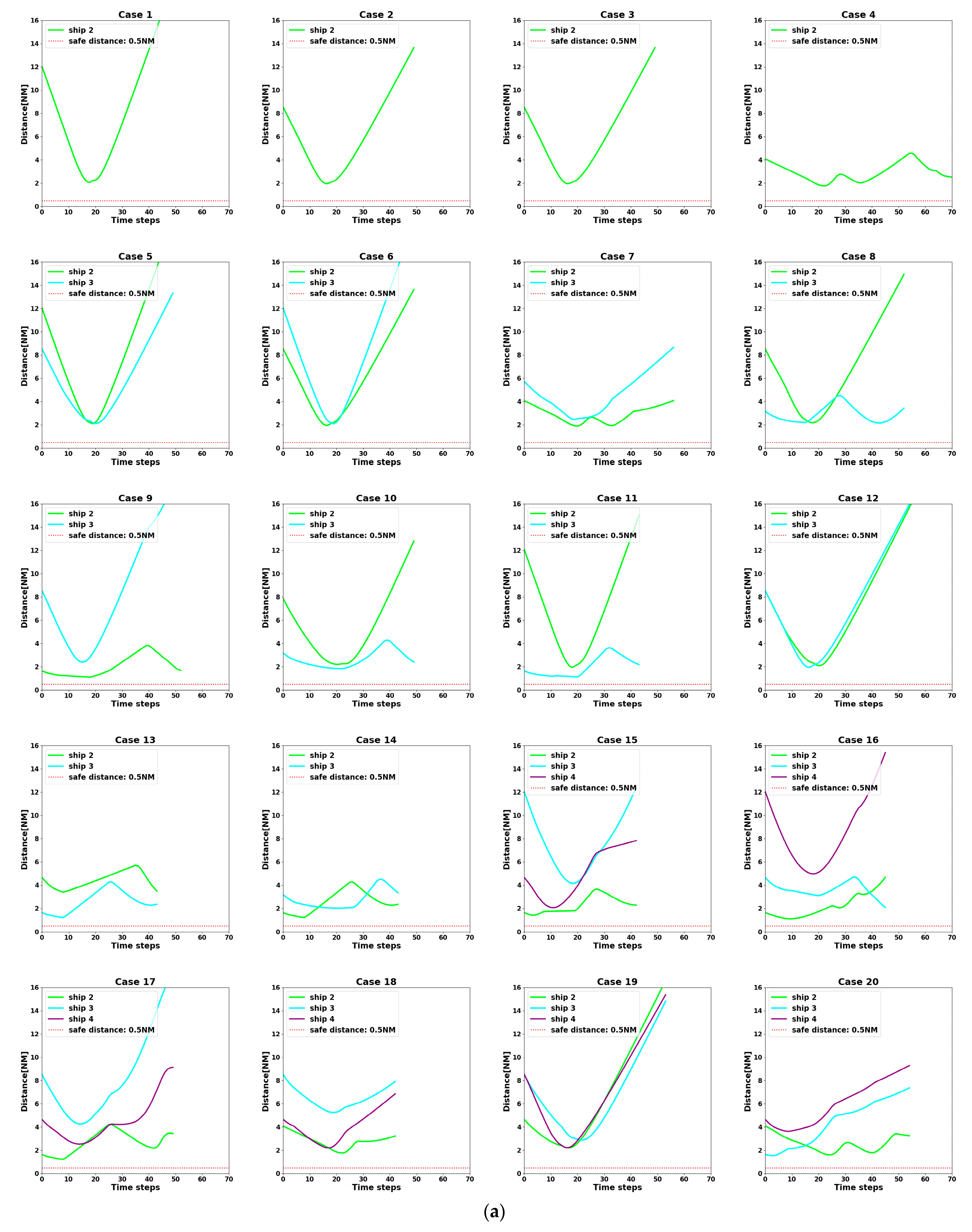
- Failure Reward: When the distance between ships is less than 0.5 NM, the algorithm defines it as a collision occurs, i.e., collision avoidance fails. Then, it will receive a larger negative reward from the environment.
- Warning Reward: When the ship moves into the collision hazard area, it will receive a small negative reward from the environment.
- Out-of-bounds Reward: When the ship enters the unplanned sea area because of taking collision avoidance actions, it will receive a medium negative reward from the environment.
- Ship Size-Sensitivity Reward: The ship’s size and sensitivity can affect the ship’s collision avoidance strategy and decision-making. Larger ships typically require a larger turning radius and longer braking distances, so ship size can be considered for inclusion in the reward function. For example, larger ships could be given more success rewards based on their size and sensitivity to emphasize their collision avoidance difficulty. This can guide different types of intelligent ships to make appropriate collision avoidance decisions for themselves.
- Success Reward: When the ship successfully avoids other ships, i.e., there is no risk of collision with any other ship at the next moment, it will receive a positive reward from the environment. This reward is refined into six components by considering all factors, i.e., rule compliance, the deviation distance at the end of the avoidance, the total magnitude of ship course changes during the avoidance process, the amount of the cumulative rudder angle during the avoidance process, the DCPA when clear of the other ship and the number of rudder operations.
- Other Reward: Except for the four cases mentioned above, the agent will not receive a reward from the environment, i.e., the reward is 0.
4. Training and Testing of Algorithm Model
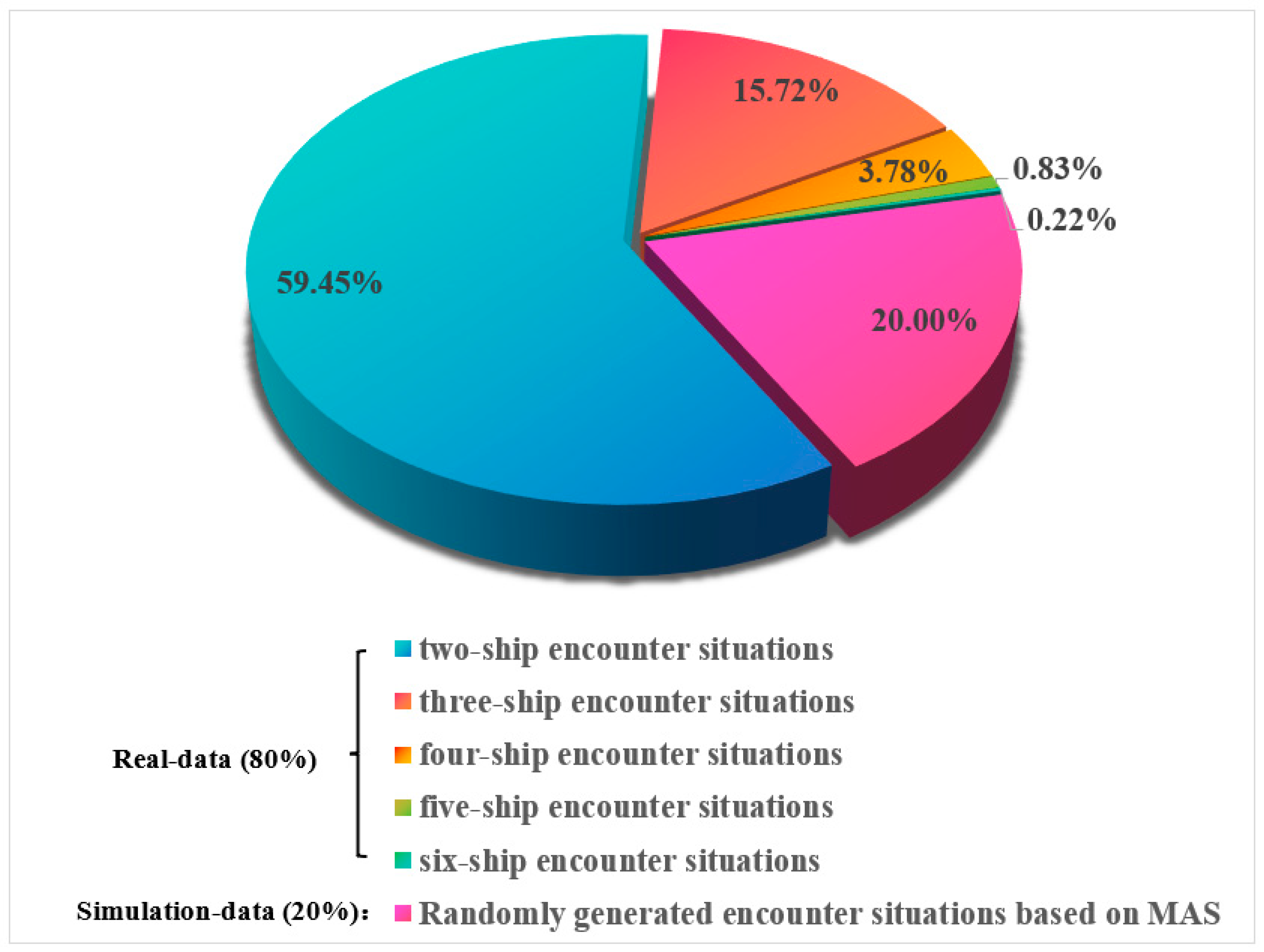
4.1. Training Set
4.1.1. Real-Data Training Set
4.1.2. Simulation Data Training Set
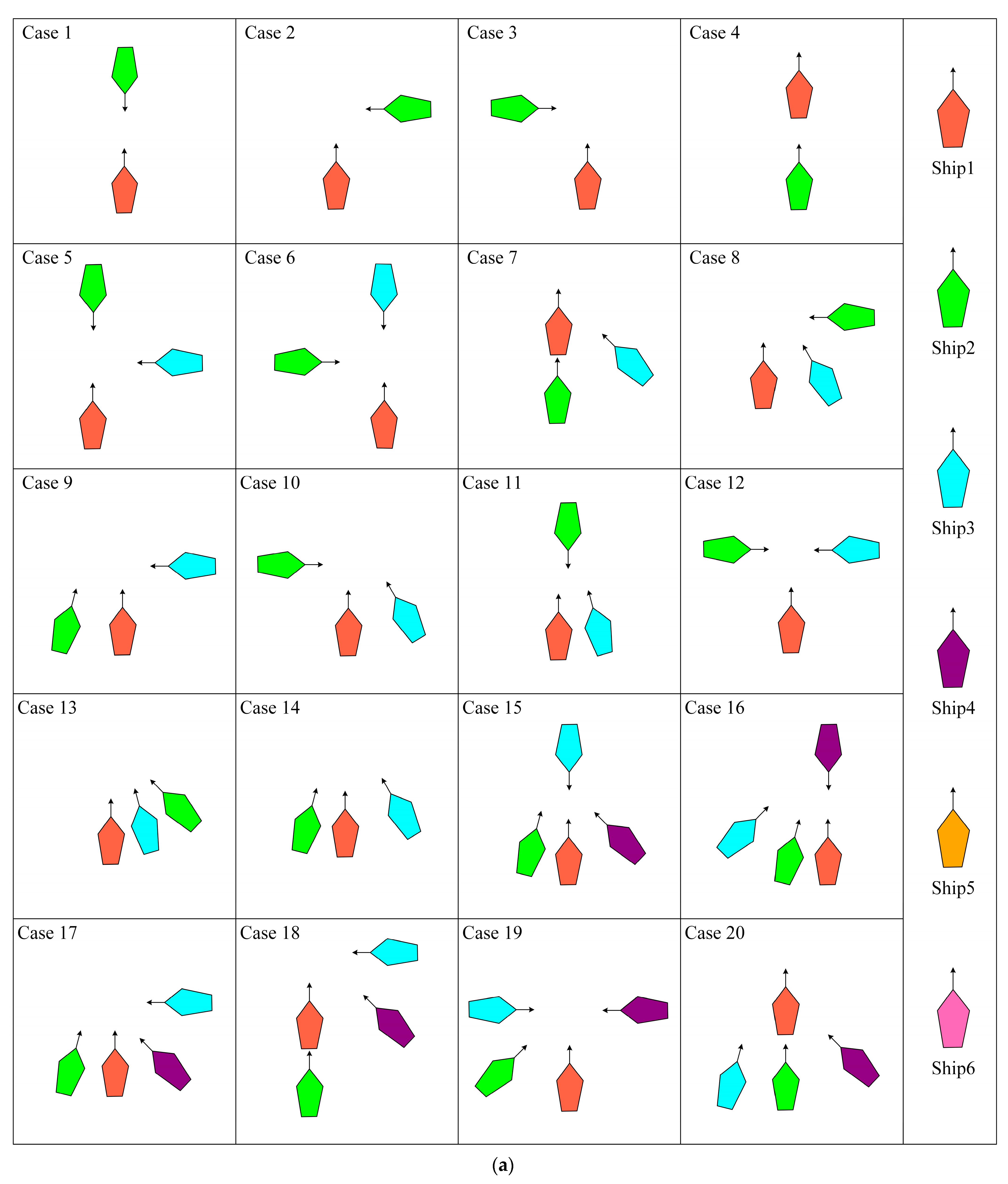
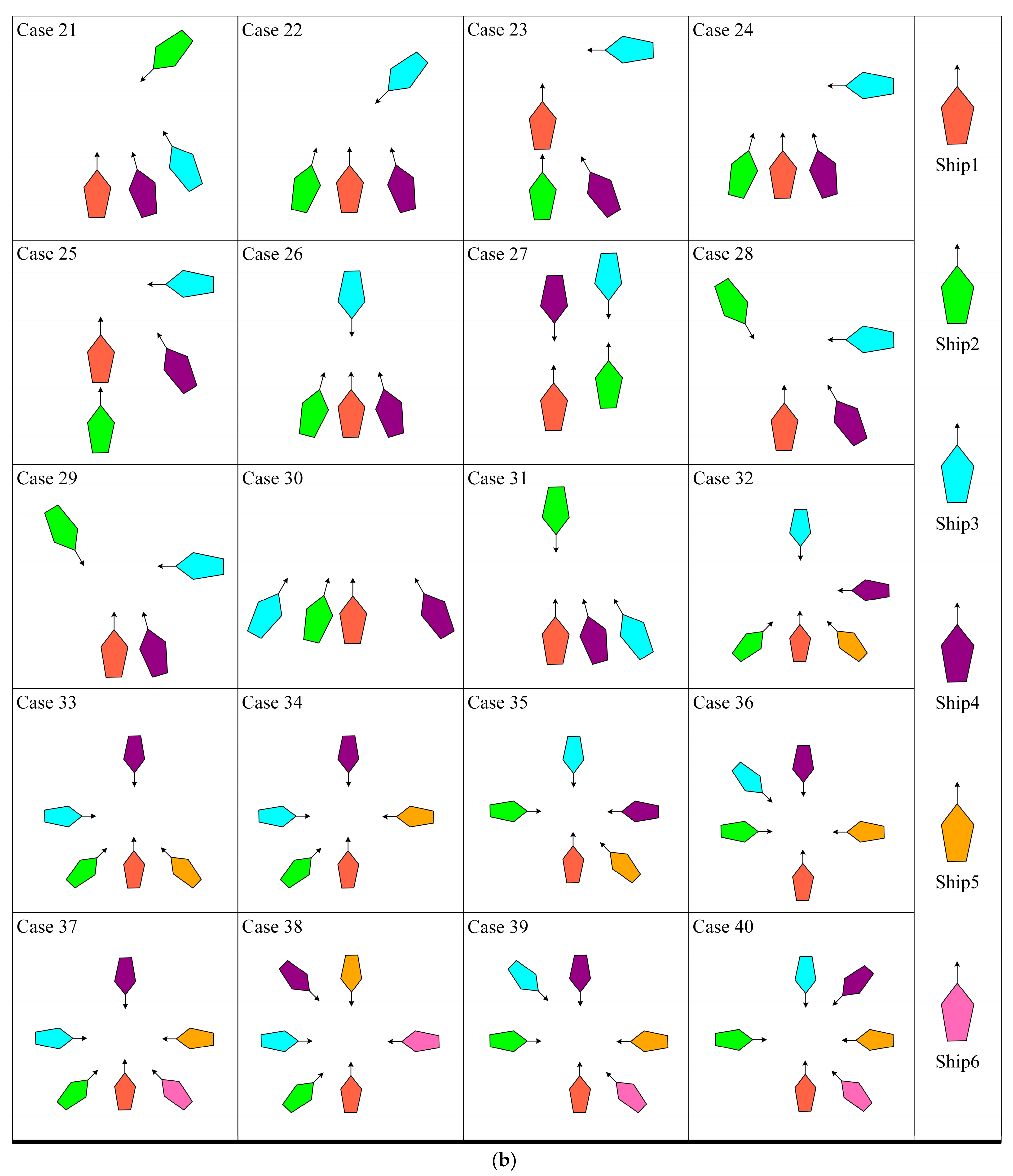
4.2. Testing Set
- Comprehensiveness extension: By testing to include a variety of possible real-world sailing scenarios, we can ensure that the algorithm is able to cope with the challenges in various aspects of actual sailing;
- Improving the model’s generalization ability: Diversified scenarios can help the model learn richer data, thus making its performance more stable and reliable in unknown environments;
- Simulating extreme situations: The particularly difficult scenarios in the encounter scenario library can simulate extreme situations that might be encountered in reality, which is essential for assessing the model’s performance under stress;
- Enhancing verification credibility: By verifying the model’s performance in various scenarios, we can more confidently ensure its safety and effectiveness in real-world applications.
- At t = 0–600 s, ship three does not perceive a hazard in the environment, the observed state is 0, and the ship is sailing towards its destination on the prescribed course;
- At t = 600 s, ship three recognizes the hazard in the environment, at which time the observation state changes to one, and collision avoidance action is started. The algorithmic model selects , , , sequentially as actions in the action space based on the policy function π;
- Until t = 1700 s, the ship removes the collision hazard by four course changes. At the same time, the observation state becomes 0. The collision avoidance decision-making switch is turned off, and the ship starts to return to the planned route;
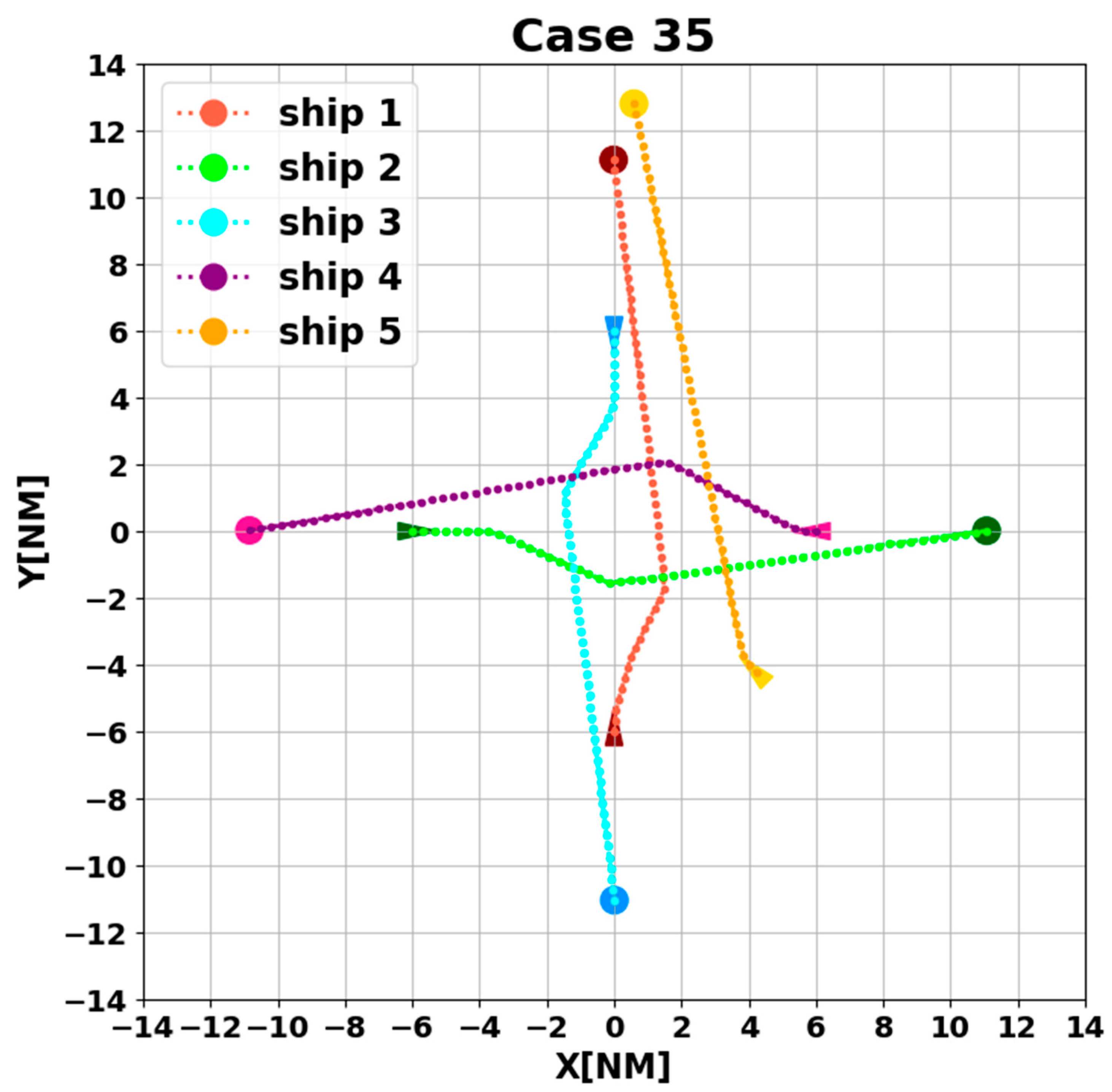
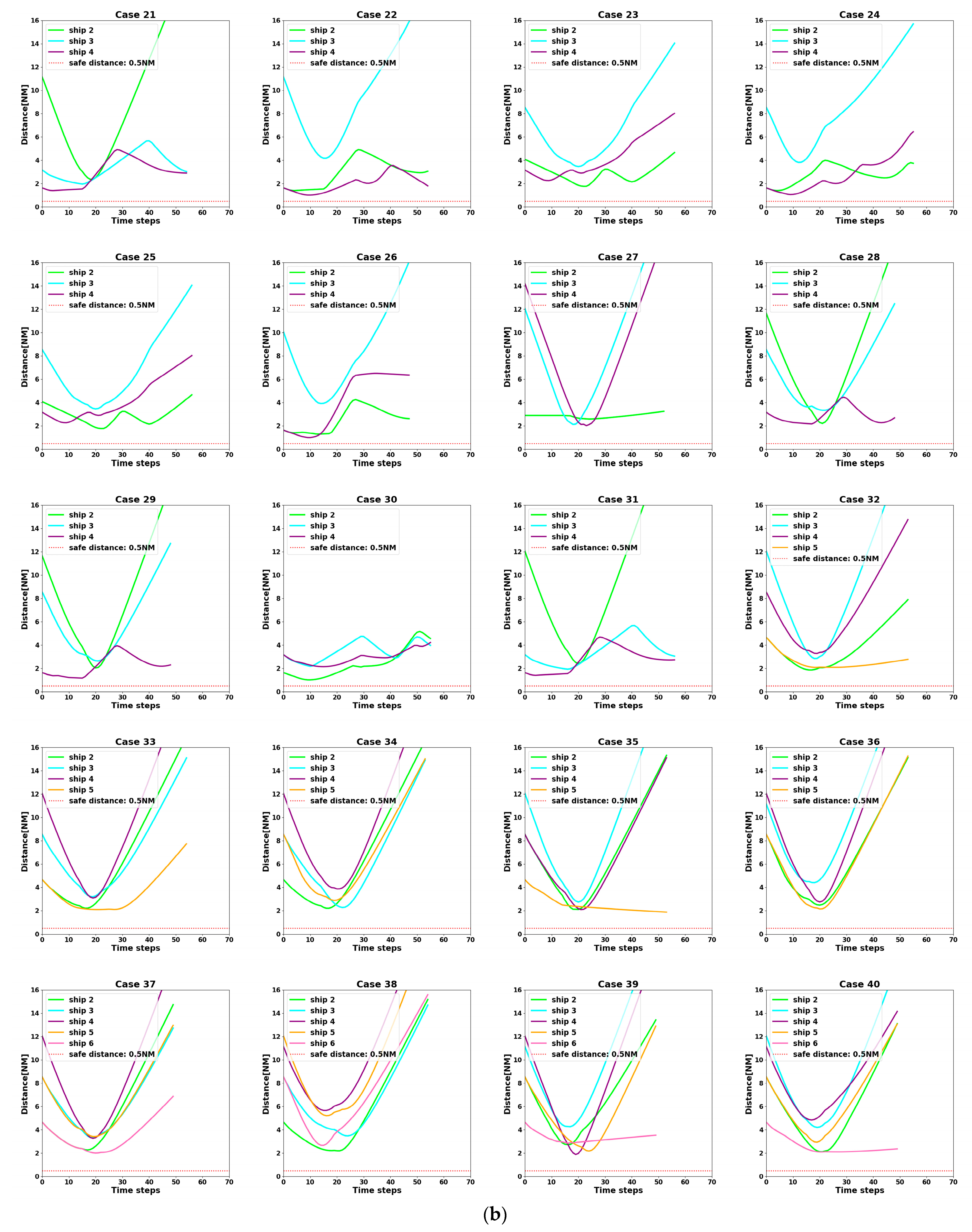
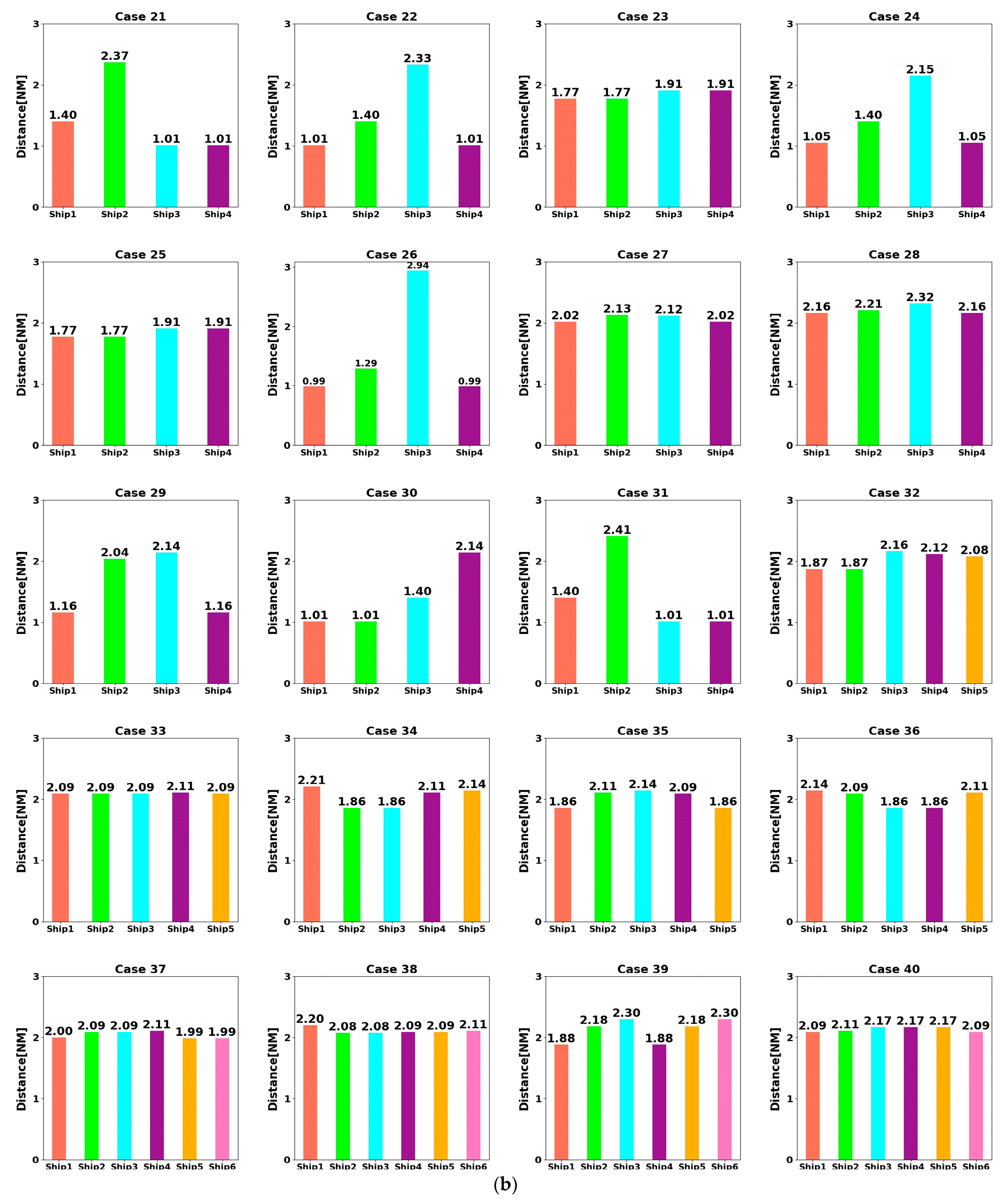
- At t = 5400 s, all ships arrive at their destinations, and the sailing missions are over. The minimum passing distances of each ship from other ships are respectively 1.86 NM, 2.11 NM, 2.14 NM, 2.09 NM, and 1.86 NM. All ships are guaranteed to complete the collision avoidance decision-making beyond the safe distance.
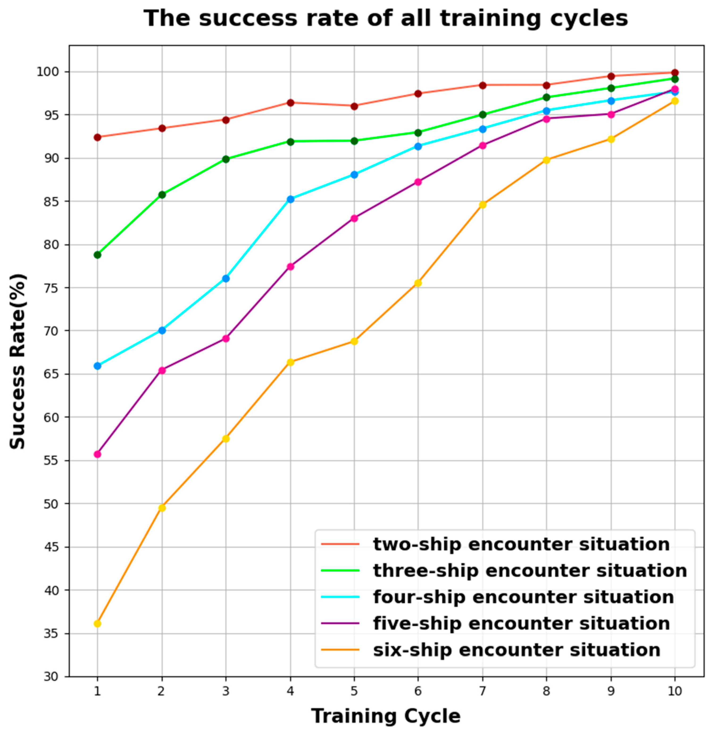
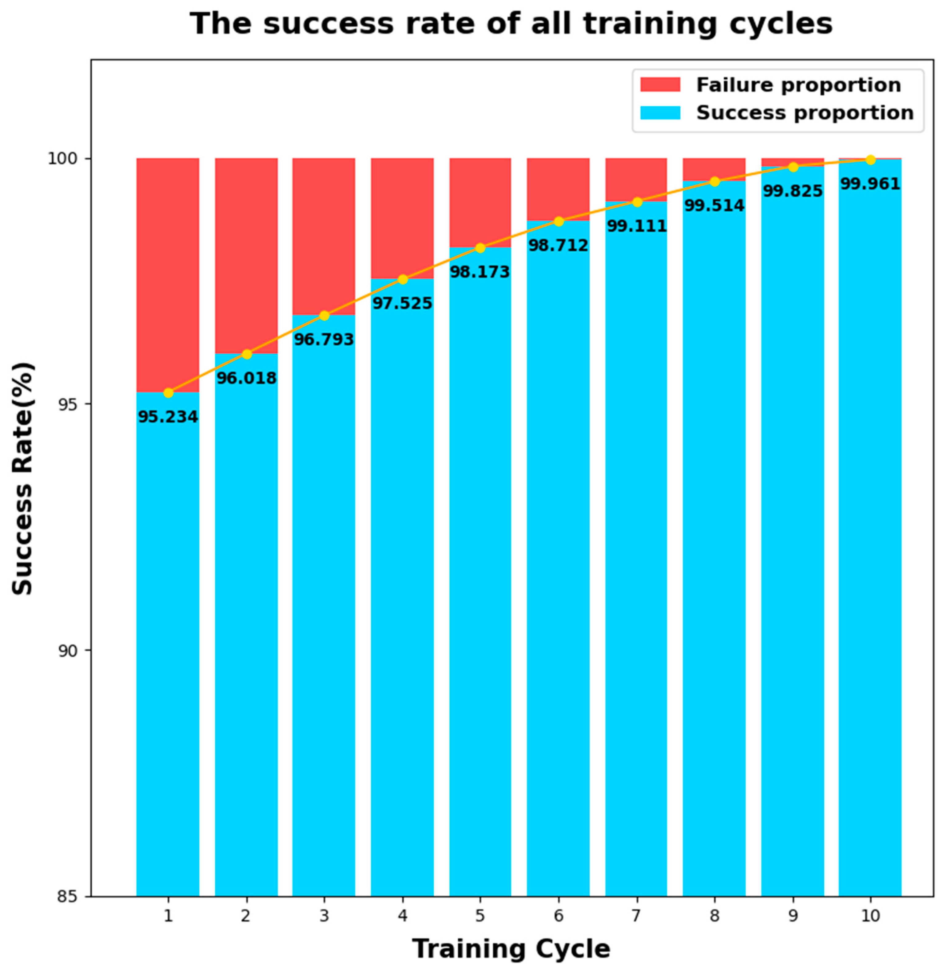
4.3. Analysis of Experimental Results
5. Conclusions
Author Contributions
Funding
Institutional Review Board Statement
Informed Consent Statement
Data Availability Statement
Conflicts of Interest
Appendix A


References
- European Maritime Safety Agency. Annual Overview of Marine Casualties and Incidents 2021; EMSA: Lisbon, Portugal, 2021; Available online: https://www.emsa.europa.eu/newsroom/latest-news/item/4266-annual-overview-of-marine-casualties-and-incidents-2020.html (accessed on 11 August 2023).
- Maritime Safety Committee. Report of the Maritime Safety Committee on Its Ninety-Ninth Session; IMO: London, UK, 2018; Available online: https://www.imo.org/en/MediaCentre/MeetingSummaries/Pages/MSC-99th-session.aspx (accessed on 16 August 2023).
- Wei, G.; Kuo, W. COLREGs-Compliant Multi-Ship Collision Avoidance Based on Multi-Agent Reinforcement Learning Technique. J. Mar. Sci. Eng. 2022, 10, 1431. [Google Scholar] [CrossRef]
- Zhang, Y.; Zhai, P. Research progress and trend of autonomous collision avoidance technology for marine ships. J. Dalian Marit. Univ. 2022, 48, 1–11. [Google Scholar]
- Papadimitrakis, M.; Stogiannos, M.; Sarimveis, H.; Alexandridis, A. Multi-Ship Control and Collision Avoidance Using MPC and RBF-Based Trajectory Predictions. Sensors 2021, 21, 6959. [Google Scholar] [CrossRef]
- Shaobo, W.; Yingjun, Z.; Lianbo, L. A collision avoidance decision-making system for autonomous ship based on modified velocity obstacle method. Ocean Eng. 2020, 215, 107910. [Google Scholar] [CrossRef]
- Huang, Y.; Chen, L.; van Gelder, P.H.A.J.M. Generalized velocity obstacle algorithm for preventing ship collisions at sea. Ocean Eng. 2019, 173, 142–156. [Google Scholar] [CrossRef]
- Ma, J.; Su, Y.; Xiong, Y.; Zhang, Y.; Yang, X. Decision-making method for collision avoidance of ships in confined waters based on velocity obstacle and artificial potential field. China Saf. Sci. J. 2020, 30, 60–66. [Google Scholar] [CrossRef]
- Singh, Y.; Sharma, S.; Sutton, R.; Hatton, D.; Khan, A. A Constrained A* Approach towards Optimal Path Planning for an Unmanned Surface Vehicle in a Maritime Environment Containing Dynamic Obstacles and Ocean Currents. Ocean Eng. 2018, 169, 187–201. [Google Scholar] [CrossRef]
- Ahn, J.-H.; Rhee, K.-P.; You, Y.-J. A study on the collision avoidance of a ship using neural networks and fuzzy logic. Appl. Ocean Res. 2012, 37, 162–173. [Google Scholar] [CrossRef]
- Szłapczyński, R.; Ghaemi, H. Framework of an evolutionary multi-objective optimisation method for planning a safe trajectory for a marine autonomous surface ship. Pol. Marit. Res. 2019, 26, 69–79. [Google Scholar] [CrossRef]
- Statheros, T.; Howells, G.; Maier, K.M.D. Autonomous ship collision avoidance navigation concepts, technologies and techniques. J. Navig. 2008, 61, 129–142. [Google Scholar] [CrossRef]
- Wang, C.; Zhang, X.; Cong, L.; Li, J.; Zhang, J. Research on Intelligent Collision Avoidance Decision-Making of Unmanned Ship in Unknown Environments. Evol. Syst. 2019, 10, 649–658. [Google Scholar] [CrossRef]
- Sun, Z.; Fan, Y.; Wang, G. An Intelligent Algorithm for USVs Collision Avoidance Based on Deep Reinforcement Learning Approach with Navigation Characteristics. J. Mar. Sci. Eng. 2023, 11, 812. [Google Scholar] [CrossRef]
- Shen, H.; Hashimoto, H.; Matsuda, A.; Taniguchi, Y.; Terada, D.; Guo, C. Automatic collision avoidance of multiple ships based on deep Q-learning. Appl. Ocean Res. 2019, 86, 268–288. [Google Scholar] [CrossRef]
- Sawada, R.; Sato, K.; Majima, T. Automatic Ship Collision Avoidance Using Deep Reinforcement Learning with LSTM in Continuous Action Spaces. J. Mar. Sci. Technol. 2021, 26, 509–524. [Google Scholar] [CrossRef]
- Zhao, L.; Roh, M.-I. COLREGs-compliant multiship collision avoidance based on deep reinforcement learning. Ocean Eng. 2019, 191, 106436. [Google Scholar] [CrossRef]
- Sutton, R.S.; McAllester, D.; Singh, S.; Mansour, Y. Policy gradient methods for reinforcement learning with function approximation. Adv. Neural Inf. Process. Syst. 1999, 12, 1057–1063. [Google Scholar]
- Luis, S.Y.; Reina, D.G.; Marin, S.L.T. A Multiagent Deep Reinforcement Learning Approach for Path Planning in Autonomous Surface Vehicles: The Ypacaraí Lake Patrolling Case. IEEE Access 2021, 9, 17084–17099. [Google Scholar] [CrossRef]
- Chen, C.; Ma, F.; Xu, X.; Chen, Y.; Wang, J. A Novel Ship Collision Avoidance Awareness Approach for Cooperating Ships Using Multi-Agent Deep Reinforcement Learning. J. Mar. Sci. Eng. 2021, 9, 1056. [Google Scholar] [CrossRef]
- Zhu, F.; Ma, Z. Ship trajectory online compression algorithm considering handling patterns. IEEE Access 2021, 9, 70182–70191. [Google Scholar] [CrossRef]
- The International Maritime Organization (IMO). Convention on the International Regulations for Preventing Collisions at Sea (COLREGs). 1972. Available online: https://www.imo.org/fr/about/Conventions/Pages/COLREG.aspx (accessed on 21 August 2023).
- Belcher, P. A sociological interpretation of the COLREGS. J. Navig. 2002, 55, 213–224. [Google Scholar] [CrossRef]
- Zhu, F.; Zhou, Z.; Lu, H. Randomly Testing an Autonomous Collision Avoidance System with Real-World Ship Encounter Scenario from AIS Data. J. Mar. Sci. Eng. 2022, 10, 1588. [Google Scholar] [CrossRef]
- Wang, X.; Zhang, Y.; Liu, Z.; Wang, S.; Zou, Y. Design of Multi-Modal Ship Mobile Ad Hoc Network under the Guidance of an Autonomous Ship. J. Mar. Sci. Eng. 2023, 11, 962. [Google Scholar] [CrossRef]
- Mnih, V.; Kavukcuoglu, K.; Silver, D.; Rusu, A.A.; Veness, J.; Bellemare, M.G.; Graves, A.; Riedmiller, M.; Fidjeland, A.K.; Ostrovski, G.; et al. Human-level control through deep reinforcement learning. Nature 2015, 518, 529–533. [Google Scholar] [CrossRef] [PubMed]
- Van Hasselt, H.; Guez, A.; Silver, D. Deep Reinforcement Learning with Double Q-Learning. In Proceedings of the 30th Association-for-the-Advancement-of-Artificial-Intelligence (AAAI) Conference on Artificial Intelligence, Phoenix, AZ, USA, 12–17 February 2016; pp. 2094–2100. [Google Scholar] [CrossRef]
- Schaul, T.; Quan, J.; Antonoglou, I.; Silver, D. Prioritized Experience Replay. In Proceedings of the 4th International Conference on Learning Representations, San Juan, PR, USA, 2–4 May 2016. [Google Scholar] [CrossRef]
- Fukuto, J.; Imazu, H. New Collision Alarm Algorithm Using Obstacle Zone by Target (OZT). IFAC Proc. Vol. 2013, 46, 91–96. [Google Scholar] [CrossRef]
- Zhang, W.; Feng, X.; Qi, Y.; Shu, F.; Zhang, Y.; Wang, Y. Towards a model of regional vessel near-miss collision risk assessment for open waters based on AIS data. J. Navig. 2019, 72, 1449–1468. [Google Scholar] [CrossRef]
- Yoo, Y.; Lee, J.-S. Evaluation of ship collision risk assessments using environmental stress and collision risk models. Ocean Eng. 2019, 191, 106527. [Google Scholar] [CrossRef]
- Zhai, P.; Zhang, Y.; Shaobo, W. Intelligent Ship Collision Avoidance Algorithm Based on DDQN with Prioritized Experience Replay under COLREGs. J. Mar. Sci. Eng. 2022, 10, 585. [Google Scholar] [CrossRef]
- Fossen, T.I. Guidance and Control of Ocean Vehicles; John Wiley & Sons Inc.: Hoboken, NJ, USA, 1994. [Google Scholar]
- Liu, J.; Zhao, B.; Li, L. Collision Avoidance for Underactuated Ocean-Going Vessels Considering COLREGs Constraints. IEEE Access 2021, 9, 145943–145954. [Google Scholar] [CrossRef]


| The Interval for Random Number Generation | Probability of Selecting the Interval |
|---|---|
| [0.0, 0.2] | 0.10 |
| [0.2, 0.4] | 0.20 |
| [0.4, 0.6] | 0.40 |
| [0.6, 0.8] | 0.20 |
| [0.8, 1.0] | 0.10 |
| Type | Action Selection | Value Evaluation |
|---|---|---|
| Nature-DQN | DQN: | Target Network: |
| Target Network | Target Network: | Target Network: |
| DDQN | DQN: | Target Network: |
| Number of Ships | Episodes | ||||
|---|---|---|---|---|---|
| Two | 67,849 | 118 | 575 | 400 | 1000 |
| Three | 17,940 | 65 | 276 | 200 | 500 |
| Four | 4316 | 26 | 166 | 100 | 200 |
| Five | 951 | 19 | 50 | 50 | 50 |
| Six | 248 | 31 | 8 | 8 | 25 |
| Integer Interval Indicating the Number of Ships | Probability of Each Element in the Interval Being Selected |
|---|---|
| [2, 3] | 0.05 |
| [4, 5, 6] | 0.15 |
| [7, 8, 9] | 0.10 |
| [10, 11, 12] | 0.05 |
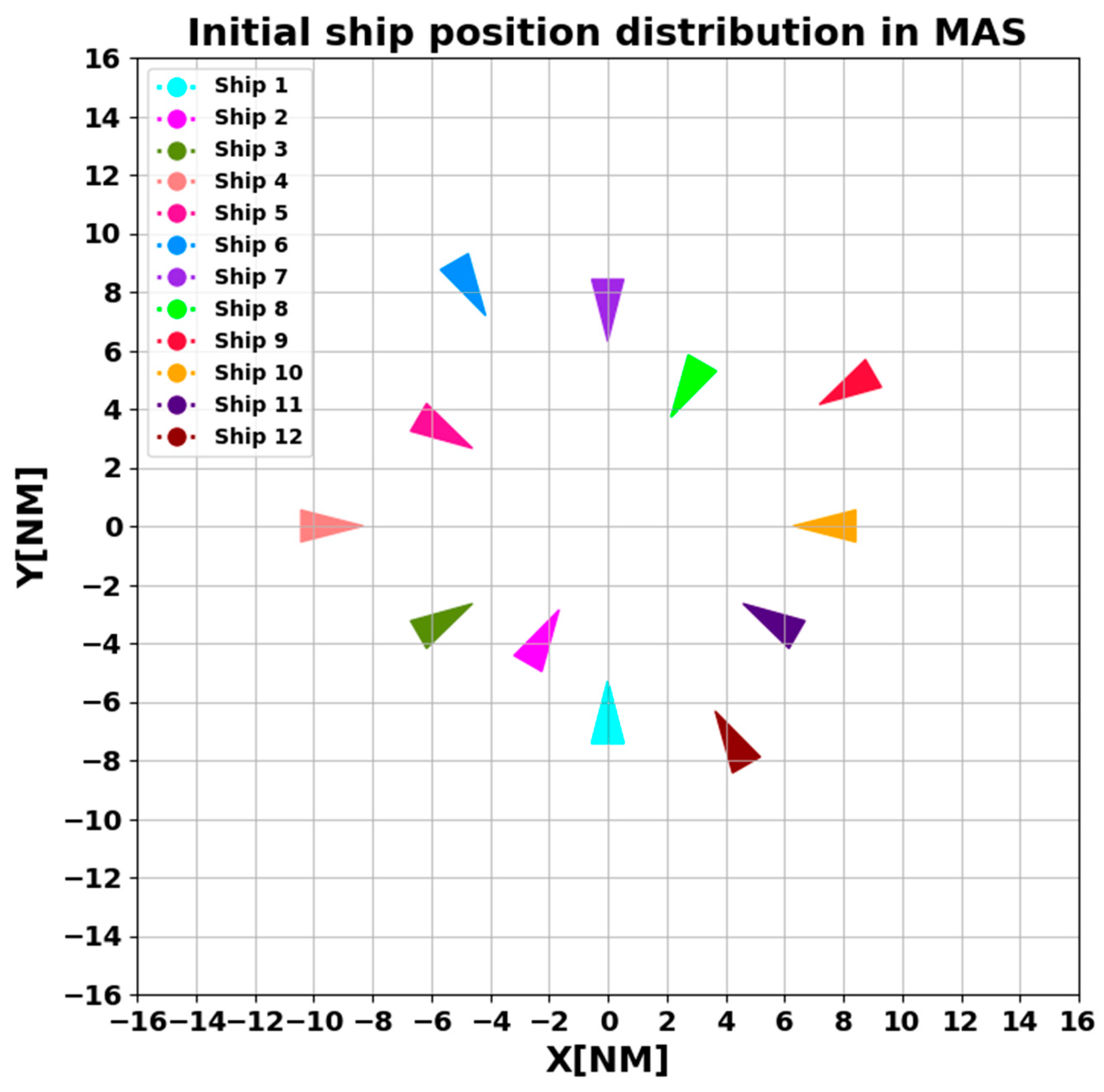
| Ship 1 | [355, 5] | 0.000 | 0.000 |
| Ship 2 | [25, 35] | −2.500 | −4.330 |
| Ship 3 | [55, 65] | −6.062 | −3.500 |
| Ship 4 | [85, 95] | −10.000 | 0.000 |
| Ship 5 | [115, 125] | −6.062 | 3.500 |
| Ship 6 | [145, 155] | −5.000 | 8.660 |
| Ship 7 | [175, 185] | 0.000 | 8.000 |
| Ship 8 | [205, 215] | 3.000 | 5.196 |
| Ship 9 | [235, 245] | 8.660 | 5.000 |
| Ship 10 | [265, 275] | 8.000 | 0.000 |
| Ship 11 | [295, 305] | 6.062 | −3.500 |
| Ship 12 | [325, 335] | 4.500 | −7.794 |
| Physical Quantity | Symbol | Numerical Value |
|---|---|---|
| Length between perpendiculars (m) | 105 | |
| Breadth (m) | 18 | |
| Speed (kn) | 12 | |
| Draft (m) | 5.4 | |
| Turning ability index (1/s) | −0.2257 | |
| Following index (s) | 86.8150 | |
| Controller gain coefficient (-) | 2.2434 | |
| Controller differential coefficient (-) | 35.9210 |
| Case No. | Ship 1 | Ship 2 | Ship 3 | Ship 4 | Ship 5 | Ship 6 | ||||||||||||
|---|---|---|---|---|---|---|---|---|---|---|---|---|---|---|---|---|---|---|
| X | Y | ψ (°) | X | Y | ψ (°) | X | Y | ψ (°) | X | Y | ψ (°) | X | Y | ψ (°) | X | Y | ψ (°) | |
| 1 | 0.000 | −6.000 | 000 | 0.000 | 6.000 | 180 | - | - | - | - | - | - | - | - | - | - | - | - |
| 2 | 0.000 | −6.000 | 000 | 6.000 | 0.000 | 270 | - | - | - | - | - | - | - | - | - | - | - | - |
| 3 | 0.000 | −6.000 | 000 | −6.000 | 0.000 | 090 | - | - | - | - | - | - | - | - | - | - | - | - |
| 4 | 0.000 | −6.000 | 000 | 0.000 | 10.000 | 000 | - | - | - | - | - | - | - | - | - | - | - | - |
| 5 | 0.000 | −6.000 | 000 | 0.000 | 6.000 | 180 | 6.000 | 0.000 | 270 | - | - | - | - | - | - | - | - | - |
| 6 | 0.000 | −6.000 | 000 | −6.000 | 0.000 | 090 | 0.000 | 6.000 | 180 | - | - | - | - | - | - | - | - | - |
| 7 | 0.000 | −6.000 | 000 | 0.000 | −10.000 | 000 | 5.657 | 5.657 | 315 | - | - | - | - | - | - | - | - | - |
| 8 | 0.000 | −6.000 | 000 | 6.000 | 0.000 | 270 | 3.000 | −5.196 | 330 | - | - | - | - | - | - | - | - | - |
| 9 | 0.000 | −6.000 | 000 | −1.553 | −5.796 | 015 | 6.000 | 0.000 | 270 | - | - | - | - | - | - | - | - | - |
| 10 | 0.000 | −6.000 | 000 | −5.000 | 0.000 | 090 | 3.000 | −5.196 | 330 | - | - | - | - | - | - | - | - | - |
| 11 | 0.000 | −6.000 | 000 | 0.000 | 7.000 | 180 | 1.553 | −5.796 | 345 | - | - | - | - | - | - | - | - | - |
| 12 | 0.000 | −6.000 | 000 | −6.000 | 0.000 | 090 | 6.000 | 0.000 | 270 | - | - | - | - | - | - | - | - | - |
| 13 | 0.000 | −6.000 | 000 | 4.243 | −4.243 | 315 | 1.553 | −5.796 | 345 | - | - | - | - | - | - | - | - | - |
| 14 | 0.000 | −6.000 | 000 | −1.553 | −5.796 | 015 | 3.000 | −5.196 | 330 | - | - | - | - | - | - | - | - | - |
| 15 | 0.000 | −6.000 | 000 | −1.553 | −5.796 | 015 | 0.000 | 6.000 | 180 | 4.243 | −4.243 | 315 | - | - | - | - | - | - |
| 16 | 0.000 | −6.000 | 000 | −1.553 | −5.796 | 015 | −4.243 | −4.243 | 045 | 0.000 | 6.000 | 180 | - | - | - | - | - | - |
| 17 | 0.000 | −6.000 | 000 | −1.553 | −5.796 | 015 | 6.000 | 0.000 | 270 | 4.243 | 4.243 | 315 | - | - | - | - | - | - |
| 18 | 0.000 | −6.000 | 000 | 0.000 | −10.000 | 000 | 6.000 | 0.000 | 270 | 4.243 | −4.243 | 315 | - | - | - | - | - | - |
| 19 | 0.000 | −6.000 | 000 | −4.243 | −4.243 | 045 | −6.000 | 0.000 | 090 | 6.000 | 0.000 | 270 | - | - | - | - | - | - |
| 20 | 0.000 | −6.000 | 000 | 0.000 | −10.000 | 000 | −1.553 | −5.796 | 015 | 4.243 | −4.243 | 315 | - | - | - | - | - | - |
| 21 | 0.000 | −6.000 | 000 | 4.243 | 4.243 | 225 | 3.000 | −5.196 | 330 | 1.553 | −5.796 | 345 | - | - | - | - | - | - |
| 22 | 0.000 | −6.000 | 000 | −1.553 | −5.796 | 015 | 4.243 | 4.243 | 225 | 1.553 | −5.796 | 345 | - | - | - | - | - | - |
| 23 | 0.000 | −6.000 | 000 | 0.000 | −10.000 | 000 | 6.000 | 0.000 | 270 | 3.000 | −5.196 | 345 | - | - | - | - | - | - |
| 24 | 0.000 | −6.000 | 000 | −1.553 | −5.796 | 015 | 6.000 | 0.000 | 270 | 1.553 | −5.796 | 345 | - | - | - | - | - | - |
| 25 | 0.000 | −6.000 | 000 | 0.000 | −10.000 | 000 | 6.000 | 0.000 | 270 | 3.000 | −5.196 | 330 | - | - | - | - | - | - |
| 26 | 0.000 | −6.000 | 000 | −1.553 | −5.796 | 015 | 0.000 | 4.000 | 180 | 1.553 | −5.796 | 345 | - | - | - | - | - | - |
| 27 | 0.000 | −6.000 | 000 | 2.000 | −4.000 | 000 | 0.000 | 6.000 | 180 | 2.000 | 8.000 | 180 | - | - | - | - | - | - |
| 28 | 0.000 | −6.000 | 000 | −3.000 | 5.196 | 150 | 6.000 | 0.000 | 270 | 3.000 | −5.196 | 330 | - | - | - | - | - | - |
| 29 | 0.000 | −6.000 | 000 | −3.000 | 5.196 | 150 | 6.000 | 0.000 | 270 | 1.553 | −5.796 | 345 | - | - | - | - | - | - |
| 30 | 0.000 | −6.000 | 000 | −1.553 | −5.796 | 015 | −3.000 | −5.196 | 030 | 3.000 | −5.196 | 330 | - | - | - | - | - | - |
| 31 | 0.000 | −6.000 | 000 | 0.000 | 6.000 | 180 | 3.000 | −5.196 | 330 | 1.553 | −5.796 | 345 | - | - | - | - | - | - |
| 32 | 0.000 | −6.000 | 000 | −4.243 | −4.243 | 045 | 0.000 | 6.000 | 180 | 6.000 | 0.000 | 270 | 4.243 | −4.243 | 315 | - | - | - |
| 33 | 0.000 | −6.000 | 000 | −4.243 | −4.243 | 045 | −6.000 | 0.000 | 090 | 0.000 | 6.000 | 180 | 4.243 | −4.243 | 315 | - | - | - |
| 34 | 0.000 | −6.000 | 000 | −4.243 | −4.243 | 045 | −6.000 | 0.000 | 090 | 0.000 | 6.000 | 180 | 6.000 | 0.000 | 270 | - | - | - |
| 35 | 0.000 | −6.000 | 000 | −6.000 | 0.000 | 090 | 0.000 | 6.000 | 180 | 6.000 | 0.000 | 270 | 4.243 | −4.243 | 315 | - | - | - |
| 36 | 0.000 | −6.000 | 000 | −6.000 | 0.000 | 090 | −4.243 | 4.243 | 135 | 0.000 | 6.000 | 180 | 6.000 | 0.000 | 270 | - | - | - |
| 37 | 0.000 | −6.000 | 000 | 4.243 | −4.243 | 045 | −6.000 | 0.000 | 090 | 0.000 | 6.000 | 180 | 6.000 | 0.000 | 270 | 4.243 | −4.243 | 315 |
| 38 | 0.000 | −6.000 | 000 | −4.243 | −4.243 | 045 | −6.000 | 0.000 | 090 | −4.243 | 4.243 | 135 | 0.000 | 6.000 | 180 | 6.000 | 0.000 | 270 |
| 39 | 0.000 | −6.000 | 000 | −6.000 | 0.000 | 090 | −4.243 | 4.243 | 135 | 0.000 | 6.000 | 180 | 6.000 | 0.000 | 270 | 4.243 | −4.243 | 315 |
| 40 | 0.000 | −6.000 | 000 | −6.000 | 0.000 | 090 | 0.000 | 6.000 | 180 | 4.243 | 4.243 | 225 | 6.000 | 0.000 | 270 | 4.243 | −4.243 | 315 |
Disclaimer/Publisher’s Note: The statements, opinions and data contained in all publications are solely those of the individual author(s) and contributor(s) and not of MDPI and/or the editor(s). MDPI and/or the editor(s) disclaim responsibility for any injury to people or property resulting from any ideas, methods, instructions or products referred to in the content. |
© 2023 by the authors. Licensee MDPI, Basel, Switzerland. This article is an open access article distributed under the terms and conditions of the Creative Commons Attribution (CC BY) license (https://creativecommons.org/licenses/by/4.0/).
Share and Cite
Niu, Y.; Zhu, F.; Wei, M.; Du, Y.; Zhai, P. A Multi-Ship Collision Avoidance Algorithm Using Data-Driven Multi-Agent Deep Reinforcement Learning. J. Mar. Sci. Eng. 2023, 11, 2101. https://doi.org/10.3390/jmse11112101
Niu Y, Zhu F, Wei M, Du Y, Zhai P. A Multi-Ship Collision Avoidance Algorithm Using Data-Driven Multi-Agent Deep Reinforcement Learning. Journal of Marine Science and Engineering. 2023; 11(11):2101. https://doi.org/10.3390/jmse11112101
Chicago/Turabian StyleNiu, Yihan, Feixiang Zhu, Moxuan Wei, Yifan Du, and Pengyu Zhai. 2023. "A Multi-Ship Collision Avoidance Algorithm Using Data-Driven Multi-Agent Deep Reinforcement Learning" Journal of Marine Science and Engineering 11, no. 11: 2101. https://doi.org/10.3390/jmse11112101