Development of a Graph-Based Collision Risk Situation Model for Validation of Autonomous Ships’ Collision Avoidance Systems

Abstract

In the maritime industry, the systematic validation of collision avoidance systems of autonomous ships is becoming an increasingly important issue with the development of autonomous ships. The development of collision avoidance systems for autonomous ships faces inherent risks of programming errors and has mostly been tested in limited scenarios. Despite efforts to verify these systems through scenario testing, these scenarios do not fully represent the complex nature of real-world navigation, limiting full system verification and reliability. Therefore, this study proposed a method for analyzing collision risk situations extracted from AIS data through graph-based modeling and establishing validation scenarios. This methodology categorizes collision risk scenarios according to their centrality and frequency and demonstrates how simple collision risk situations gradually evolve into harsh situations.

1. Introduction

Collision avoidance is of paramount importance in the development of autonomous ships given their significant impact on human safety, the environment, and the economy. Therefore, ensuring the reliability of their collision avoidance systems is critical [1].

Although various approaches, from kinematics to artificial intelligence, have been utilized in developing collision avoidance systems, their human design origin presents risks of programming errors due to factors such as inadequate training or program bugs. This underlines the necessity of rigorous system testing and validation [2,3,4,5,6,7,8,9,10,11,12,13,14,15,16,17,18].

The concerns and challenges in collision avoidance systems development are validated by incidents caused by system defects across various industrial domains. Issues arising from internal defects necessitate a systematic flaw elimination and thorough understanding of the collision avoidance algorithm’s critical system states to ensure safety, particularly in complex, unanticipated scenarios during operation [19,20].

The systematic development and testing of potential scenarios is inherently complex and multifaceted. Though research has identified methods for comprehensive scenario development for testing collision avoidance systems, their effectiveness in thoroughly understanding and replicating the multifaceted and varied collision risks in real navigation settings is limited, sometimes due to the increased number and complexity of the parameters involved [21,22,23,24,25,26,27,28,29,30,31,32].

Therefore, this study aims to develop a methodology for the systematic verification of autonomous ship collision avoidance systems by generating realistic collision risk situations. This methodology, while not primarily focused on the direct validation of autonomous ship collision avoidance systems, emphasizes the understanding and development of collision risk situation scenarios through the objective analysis of graph networks. It encompasses multiple collision risk situations that have occurred in the past, and thereby seeks to extract and systematize realistic scenarios of varying levels of complexity that can be useful in the evaluation of such systems in hindsight.

2. Methodology

In this section, we propose a data-driven approach to analyze ship collision risk situations (CRSs) using a graph-based model. First, CRSs satisfying certain conditions are extracted from the AIS data. Each situation is transformed into a categorical vector by a combination of “unit scenarios” that form the context of each ship. The similarity between these vectors is then translated into a matrix computed using a modified version of the Jaccard similarity. This similarity matrix is then visualized as a network graph. A detailed view of the whole process is shown in Figure 1. The ultimate goal of these steps is to gain a systematic understanding of CRSs, with more specific methods described in the following subsections.

2.1. Extraction of CRSs

This section describes the extraction of collision risk situations from AIS data in the Southern Sea of Korea from September to November 2019. The procedure commences with defining CRSs, followed by a thorough data pre-processing phase to cleanse and synchronize the AIS data, and then extracting CRSs based on specific CPA and TCPA criteria. The extracted collision risk situations are converted into a relative Cartesian coordinate system to facilitate precise comparative analysis and ensure consistency across various encounter scenarios.

2.1.1. Definition of CRSs

For this study, we define a “Collision Risk Situation” as a scenario in which one or more vessels are involved and at least one vessel meets the criteria of DCPA (distance to the closest point of approach) and TCPA (time to the closest point of approach). Although the criteria for evaluating the collision risk between vessels based on DCPA and TCPA are rather ambiguous and vary with the size of the traffic area and the ships themselves, the purpose of this study is to suggest a methodology. Therefore, we identified situations with a considerable risk of collision by using a DCPA of 0.1 nautical miles and a TCPA of 6 min. Specifically, if multiple vessels are involved and the $i$th vessel meets a condition where DCPA is 0.1 nautical miles or less and TCPA is 6 min or less, the given scenario involving that vessel and others is classified as a collision risk situation (according to Equation (1)):

$$\mathrm{CRS}=\left\{\mathrm{Exists}i\in \left(\mathrm{encountered}\mathrm{vessels}\right)\mathrm{such}\mathrm{that}\left(\mathrm{DCPA}\_i\le 0.1\right)\wedge \left(\mathrm{TCPA}\_i\le 6\right)\right\}$$

(1)

2.1.2. AIS Data

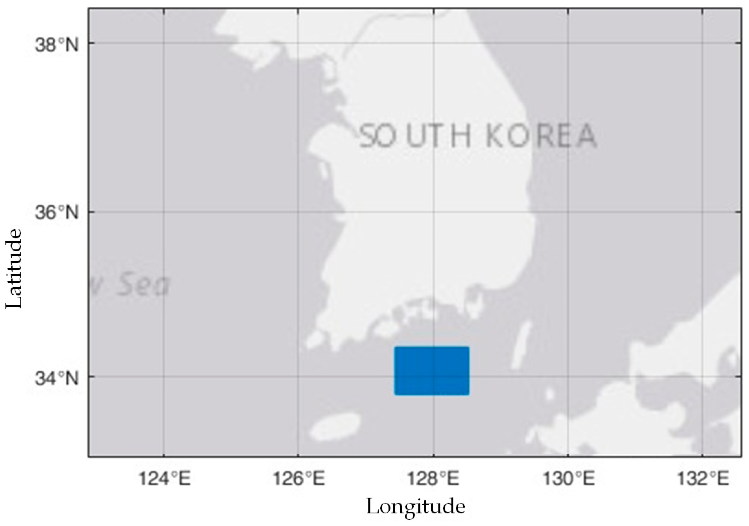
We have employed automatic identification system (AIS) data, which provides information on a vessel’s identity, location, course, and speed, and is commonly used to analyze maritime traffic. The spatial range of the data spans the Southern Sea of the Republic of Korea, a region chosen for its lack of terrestrial interference and ability to extract various vessel encounter scenarios as shown in Figure 2. The temporal range of the utilized data spans from 1 September 2019 to 30 November 2019, containing a total of 12,139,052 position data points, which were generated by 4216 vessels.

$$\begin{gathered} N33°{21}^{\prime }{00}^{″}<x_i<N34°{48}^{\prime }{00}^{″},i=1,2,\cdots ,n-1,n \\ E127°{27}^{\prime }{00}^{″}<y_i<E128°30\prime 00″ \end{gathered}$$

(2)

2.1.3. Trajectory Extraction and Data Cleaning (Pre-Processing)

AIS data, comprising navigational information collected from various vessels, form a time-series dataset. Its composition is interspersed over time and inherently contains certain inaccuracies. In this phase of the research, considering this complexity, our objective was to extract the trajectories of a specific target vessel and its surrounding vessels. To achieve this, we underwent a comprehensive data-cleaning process, which included error correction and synchronization of the time-series data.

The extraction of the subject ships and the encountering vessels was carried out via the following process. As the ongoing project supporting this study plans to develop vessels between 100 and 130 m in length, and the same length range was chosen for the subject vessels in the AIS data analysis. Subject ships were initially identified in the static data and subsequently extracted from the dynamic data. To focus on vessels actively navigating, only those with a speed exceeding 5 knots were selected. Encounter vessels were determined to be those located within 3 nautical miles of the subject ship’s trajectory during the same time frame.

The extracted ships have inconsistent time series frequencies. Due to this inconsistency, the time stamps of the own ship were regularized to one-minute intervals. For the time-varying values of position, course, speed, and heading, linear interpolation was applied during the time series data normalization process. The choice of linear interpolation was driven by a need to select an algorithm with low computational demands due to the handling of large-scale data. Additionally, excluding vessels with very high variations in speed and course—which are rare cases—linear interpolation did not exhibit notable disadvantages in results compared to other algorithms (such as spline, pchip, and makima), substantiating its application. In addition, the data of the relative ships were synchronized to match the timestamps of the subject ship, and interpolation was also applied to position, course, speed, and heading. Notably, although course and speed are key variables in discriminating the navigational relationship between the subject ship and the encountering ships, they were recalculated based on the interpolated positions due to discrepancies between them.

2.1.4. CRSs Extraction

The pre-processing performed up to this stage has synchronized the trajectory data for both the subject ship and the other ships on a minute-by-minute basis. These data serve as the basis for the extraction of CRSs, which are used to assess the risk of collision on a minute-by-minute basis. In this phase, the CPA and TCPA values were derived from each trajectory using the position, course, and speed information of the target vessel and the encountering vessel. Moments that met specific criteria for CPA and TCPA were identified, and the situation involving the encountering vessel and surrounding vessels at that time was defined and recorded as a CRS. This specific scenario was referred to in our research as a “moment situation”, which can be understood as a snapshot capturing navigational circumstances that meet certain collision risk criteria. Specifically, a “moment situation” is the specific moment satisfies the CPA and TCPA conditions between the subject and the encountering vessels, and is considered a CRS.

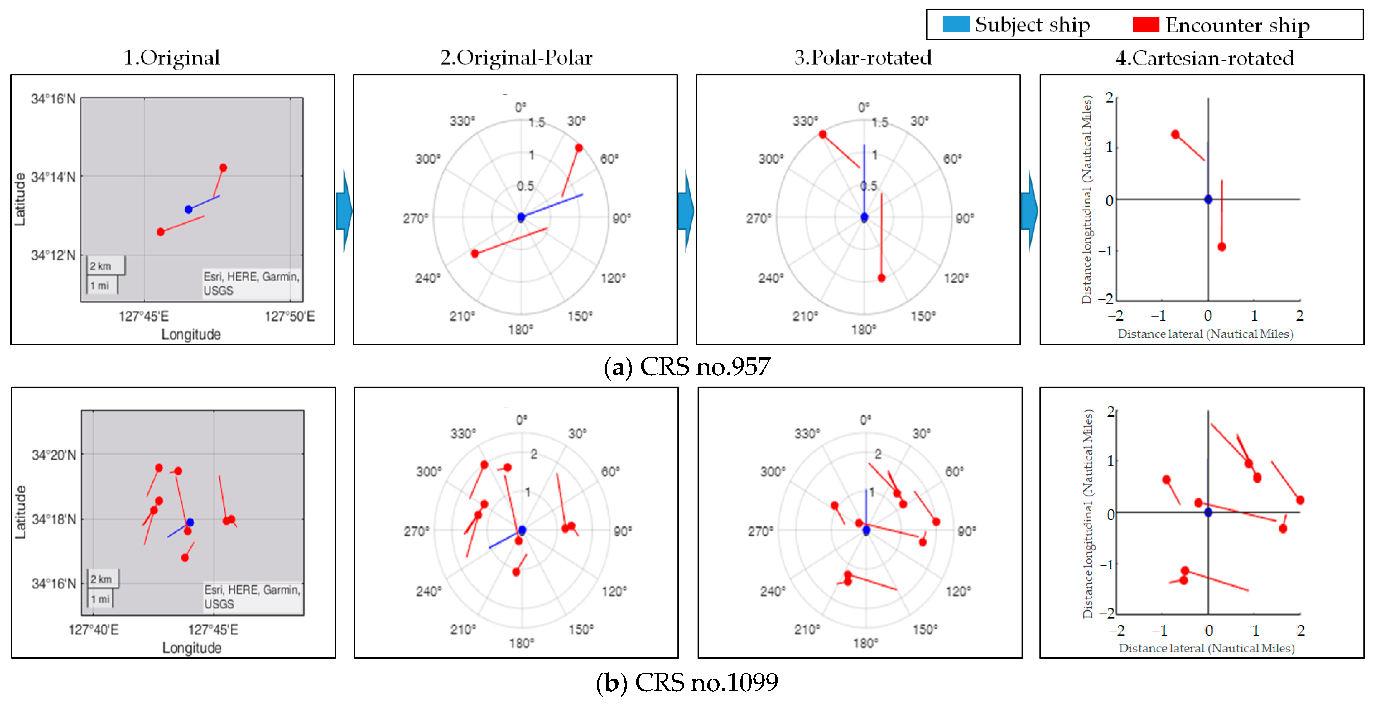
2.1.5. Converting CRSs to a Relative Cartesian Coordinate System

The extracted CRSs were detailed based on true north, describing both the ship’s trajectory and the encounter situations. To refine the comparison and analysis of these encounters, the CRSs were adjusted to a course-up orientation centered on the subject ship’s course. In addition, the subject ship was fixed at the origin (0,0) by a Cartesian coordinate system transformation, while the positions of the other ships were defined relative to it by x and y coordinates. The purpose of this transformation was not only to avoid clustering errors induced by the periodicity of the angles in the polar coordinate system and to consistently represent different collision risk situations (CRSs) under conditions relative to the subject ship; it was also to effectuate data reduction by expressing collision risk situations—previously articulated through the latitude, longitude, speed, course, and heading of the subject and encounter ships—succinctly in terms of their current and future positions.

2.2. Unit Scenario

This section introduces the concept of “unit scenarios” within CRSs, which allows for a systematic categorization of individual collision risk situations. This involves the extraction and normalization of relevant features, followed by k-means clustering to formulate distinct unit scenario groups. Finally, the CRSs are transformed into categorical vectors using unit scenario clusters to provide a compact and consistent representation that allows for detailed analysis and understanding of collision scenarios.

2.2.1. Concept of Unit Scenario

The extracted CRS not only reflects the collision risk relationship; it also comprehensively describes the maritime situation at a given time, including various parameters such as the distribution of nearby ships’ positions, draught, speed, and ship length. Taking this diversity into account, this study attempted to systematically categorize the encounter relationships of all vessels that comprise the CRS and endeavored to represent the CRS effectively by combining these interactions. To achieve this, individual encounters between ships were defined as “unit scenarios”. These scenarios were then clustered and labeled to provide a systematic categorization of encounter relationships within the CRS.

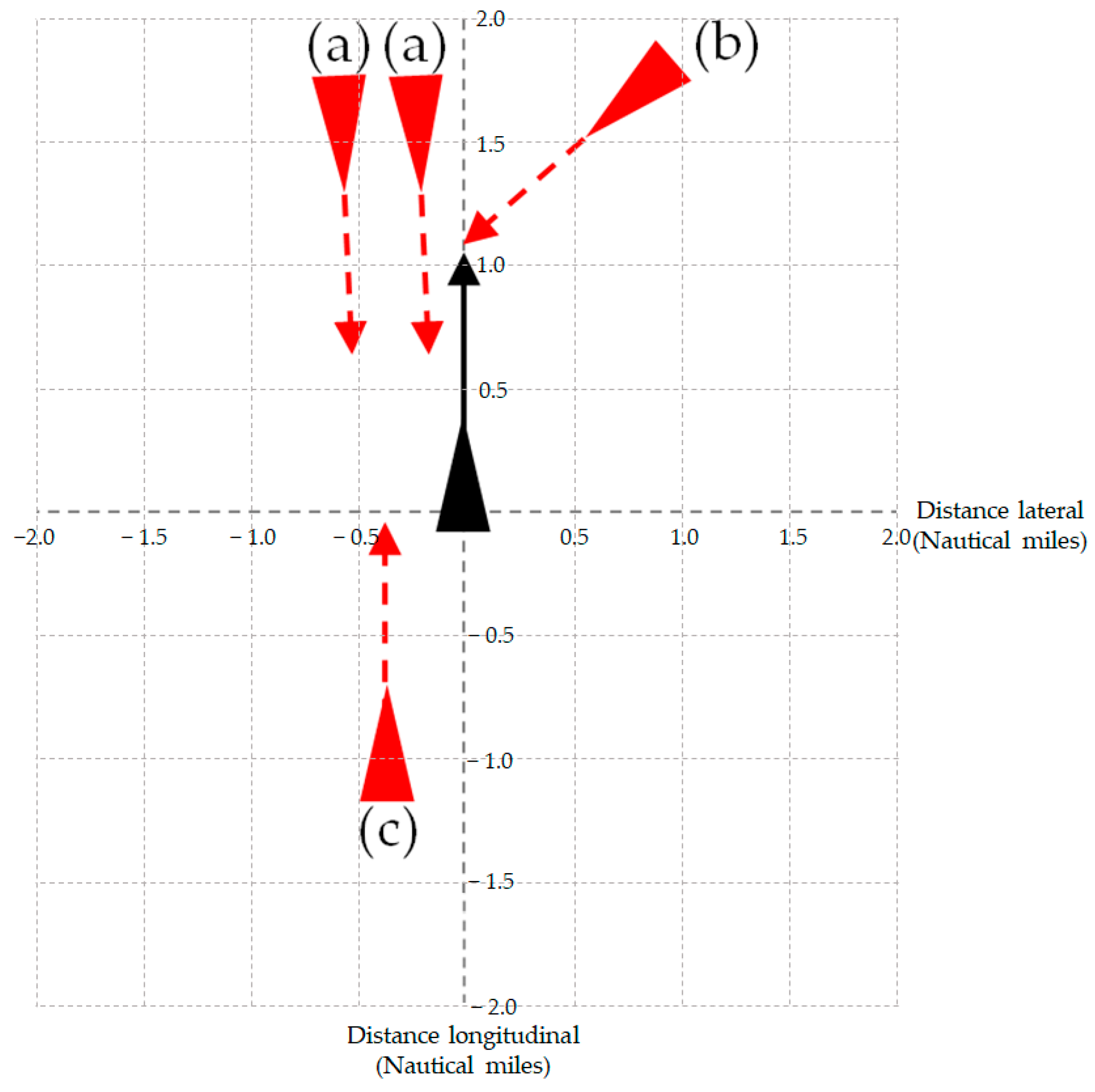
The definition of the unit scenario is as follows: it represents an individual ship’s encounter situation as separate components of the CRS. In Figure 3, the ship shown in black represents the subject ship, while the ships shown in red represent the opposing ships. The position indicated by the triangle represents the initial point that was captured as a CRS at the specified instance. In addition, the length and direction of the arrow indicate the speed and course of each ship, respectively. The endpoint of the arrow, referred to as the “terminal point,” illustrates the estimated position of the vessel after a given time interval by utilizing a vector composed of the course and speed from the AIS data of the vessel at the “initial point.” In this study, a six-minute period was used to calculate the ship’s terminal point. The CRS presented includes a total of four opposing vessels, including vessel (b), which poses a collision risk. Each of these vessels can be classified into individual unit scenarios, labeled (a), (b), and (c). According to this concept, the CRS is described as being composed of two ships corresponding to unit scenario (a), one ship to unit scenario (b), and one ship to unit scenario (c). This concept of unit scenario is utilized to describe the different types of ship encounters that compose the CRS as fine-grained categorical variables, which are finally applied as elements to vectorize the CRS.

2.2.2. Feature Engineering for Unit Scenario Clustering

For a systematic clustering of the unit scenario, it is imperative to extract and select features that effectively represent individual encounter situations. In this study, as shown in

Table 1. Extracted feature list for unit scenario clustering.

Number	Features	Description
F1	Distance (Initial)	Distance between subject ship and each encounter ship at initial point
F2	Distance (Change)	Difference between distance from terminal point and distance from initial point
F3	Relative position at initial point (Cartesian coordinate $\mathrm{x}$)	The Cartesian coordinate (x-axis) of the encounter ship at initial point: based on the subject ship as a reference, the port side is denoted by a negative value (−) and the starboard side by a positive value (+)
F4	Relative position at initial point (Cartesian coordinate $\mathrm{y}$)	The Cartesian coordinate (y-axis) of the encounter ship at the initial point: based on the subject ship as a reference, forward is denoted by a positive value (+) and aft by a negative value (−)
F5	Relative position at terminal point (Cartesian coordinate $\mathrm{x}$)	The Cartesian coordinate (x-axis) of the encounter ship at terminal point: based on the subject ship as a reference, the port side is denoted by a negative value (−) and the starboard side by a positive value (+)
F6	Relative position at terminal point (Cartesian coordinate $\mathrm{y}$)	The Cartesian coordinate (y-axis) of the encounter ship at the terminal point:bBased on the subject ship as a reference, forward is denoted by a positive value (+) and aft by a negative value (−)
F7	Encounter ship‘s course	Encounter ship‘s course at initial point
F8	Encounter ship‘s speed	Encounter ship‘s speed at initial point

, we extracted various features related to the relative position, course, distance, and speed of the encounter ship, such as the Cartesian coordinates at both the initial and terminal points based on the reference of the subject ship, the distance between the ships at the initial point, the change in distance from the initial to the terminal point, and the course direction of the encounter ship at both points. These features reflect the relative position and its changes based on the subject ship and serve as representative values for the encounter ship’s movement. After extracting these features, min–max normalization was applied to adjust for the importance bias caused by differences in the units of each feature.

The extracted and normalized features were applied to the Laplacian feature selection algorithm, and their importance was ranked based on their impact on clustering. While most features showed potential for clustering effectiveness with an importance score of 0.9 or higher, specific features were chosen to ensure computational efficiency and to facilitate intuitive interpretation of the clustering results. In particular, the features with the highest importance, F7 (initial course), F8 (initial speed), F3 (initial relative position—Cartesian coordinate x), and F4 (initial relative position—Cartesian coordinate y), were distinguished within two main domains: relative motion and position of the vessel. Due to their intuitive nature in interpreting the clustering results, these features were selected as the final features applied in clustering.

2.2.3. Unit Scenario Clustering

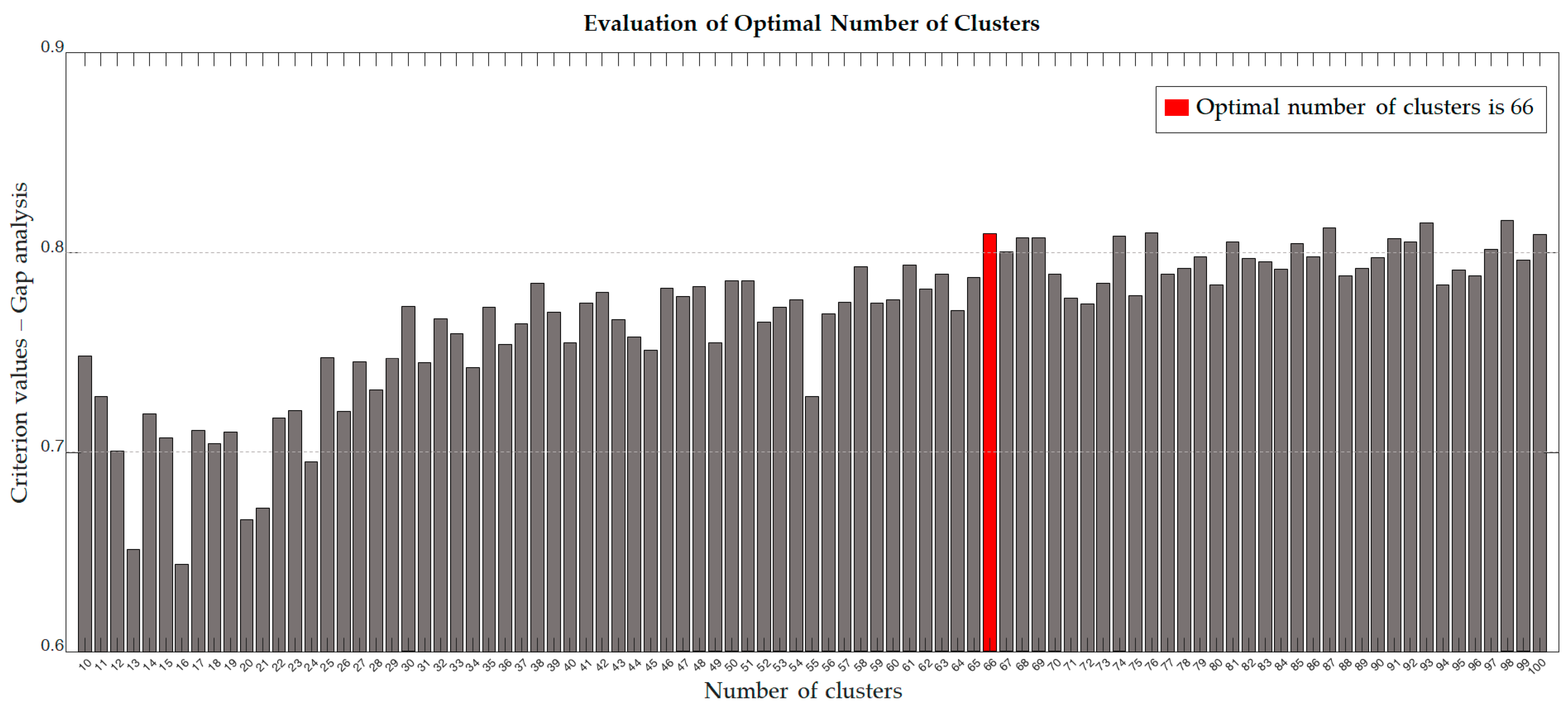
The feature matrix of the unit scenario was used in k-means clustering. To preserve the independent characteristics of each feature dimension while reducing the sensitivity to outliers, the city block distance was chosen as the distance measurement method [33]. In order to determine the optimal number of clusters, a gap analysis was conducted. Figure 4 shows a bar graph illustrating the results of this analysis. The x-axis represents the number of clusters, while the y-axis represents the gap analysis results for each cluster number. The height of the bar graph does not significantly increase beyond 66 clusters, indicating that 66 is the optimal number of clusters. Thus, the unit scenarios that make up the entire CRS were divided into 66 distinct clusters. These were then used as elements in vectors to describe each encounter situation in the next stage.

2.2.4. Vectorization of CRSs

The categorized unit scenarios are used as components of each CRS vector to effectively represent collision risk situations. This approach provides a significant advantage in minimizing information loss during the aggregation process, as it allows for the consistent representation of all encounter ships within a CRS, from single encounters to complex situations involving multiple ships, in a uniform categorical vector format. Each CRS is transformed into a categorical vector using the labels of the encounter ships that comprise it. To mitigate the loss of similarity between vectors with the same labels but in different sequences, the order of the vectors was reorganized in ascending order.

2.3. Graph-Based Modeling

In this section, a modified Jaccard similarity measure is utilized to create a similarity matrix between CRS vectors, which is then applied in graph-based modeling to visually represent the relation of CRSs. The layout and edge thickness within the graph are adjusted to intuitively convey the degree of similarity between nodes.

2.3.1. Similarity Matrix

Computing a similarity matrix between the generated vectors is an essential step for graph analysis. In this study, we used a modified Jaccard similarity measure, tailored for specific purposes, to assess the similarity between vectors. The Jaccard similarity index traditionally calculates the similarity between two vectors based on the ratio of their intersection to their union, as described by the following formula:

$$\mathrm{Jaccard}\mathrm{Similarity}\left(\mathrm{A},\mathrm{B}\right)=\frac{\left|A{{\displaystyle \cap }}^{}B\right|}{\left|A{{\displaystyle \cup }}^{}B\right|}.$$

(3)

However, this method is limited by its inadequate consideration of the total length of the arrays and their overlapping elements. To overcome these limitations, the modified Jaccard similarity was designed, which computes the similarity by dividing the number of identical elements, including duplicates, by the length of the longer of the two arrays. Thus, this modified method considers the duplicate elements that were previously ignored by the conventional Jaccard index, allowing for a more granular evaluation of similarity. The following formula represents the modified Jaccard similarity:

$$S=\frac{\min \left({{\displaystyle \sum }}_{k=1}^{\mid B\mid }{1}_{B_k\in A{{\displaystyle \cap }}^{}B},{{\displaystyle \sum }}_{k=1}^{\mid A\mid }{1}_{A_k\in A{{\displaystyle \cap }}^{}B}\right)}{\max \left(\mid A\mid ,\mid B\mid \right)},$$

(4)

where A and B are two vectors, S is the modified Jaccard similarity between them, and $1_{B_k\in A{{\displaystyle \cap }}^{}B}$ and $1_{A_k\in A{{\displaystyle \cap }}^{}B}$ are indicator functions that return 1 if $B_k$ and $A_k$ are in $A{{\displaystyle \cap }}^{}B$, respectively, and 0 otherwise. This formula calculates the modified Jaccard similarity by dividing the minimum number of elements in $A$ and $B$ that are also in their intersection by the maximum length of $A$ and $B$. This calculation allows us to measure the similarity between two vectors.

2.3.2. Parameter Setting for Graph-Based Modeling

The similarity matrix was used as an input variable for graph-based modeling, and the CRS was visualized as a graph-network. The layout of the nodes in the graph was configured by applying a force direction methodology to adjust the distance between nodes in an inverse proportion to their similarity. Based on these configurations, the length of the edges connecting the nodes was also set to be inversely proportional to the similarity between the nodes. Additionally, the thickness of the edges was set to be directly proportional to the similarity, so that the connections between nodes with high similarity were thicker. Centrality indices, utilized to portray the connectivity among nodes, encompass “Degree Centrality,” which indicates the number of direct connections a node maintains; ‘Closeness Centrality,” representing the average shortest path length across all nodes; and “Betweenness Centrality,” expressing the frequency at which a node appears on the shortest paths between every pair of nodes [34]. For this study, “Degree Centrality” was employed to determine the direct connections each CRS node has with other nodes.

3. Result

This section describes the results of the application of the methodology presented in this study. The results section consists of results and examples of extracted CRSs, results of vectorization of CRSs, and results of graph-based modeling.

3.1. Extracted CRSs

In this study, we analyzed ship traffic data collected over a three-month period and identified a total of 1205 collision risk situations (CRS). When the subject ship encountered various other ships during its sailing, if even one other ship met the conditions for a collision risk, the entire interaction involving the subject ship and its surrounding ships at that moment was extracted as a CRS. According to this methodology, each CRS necessarily incorporates at least one vessel with a collision risk. Figure 5 presents an analysis based on the number of vessels involved in the encounter, illustrating situations ranging from encounters with a relatively small number of other vessels to situations with multiple vessels, exemplified by cases such as CRS no.957 and no.1099. From the analysis, in each situation, at least one vessel posed a collision risk. These data were then processed and visualized centering on the subject ship using a course up display.

3.2. Vectorization of CRSs

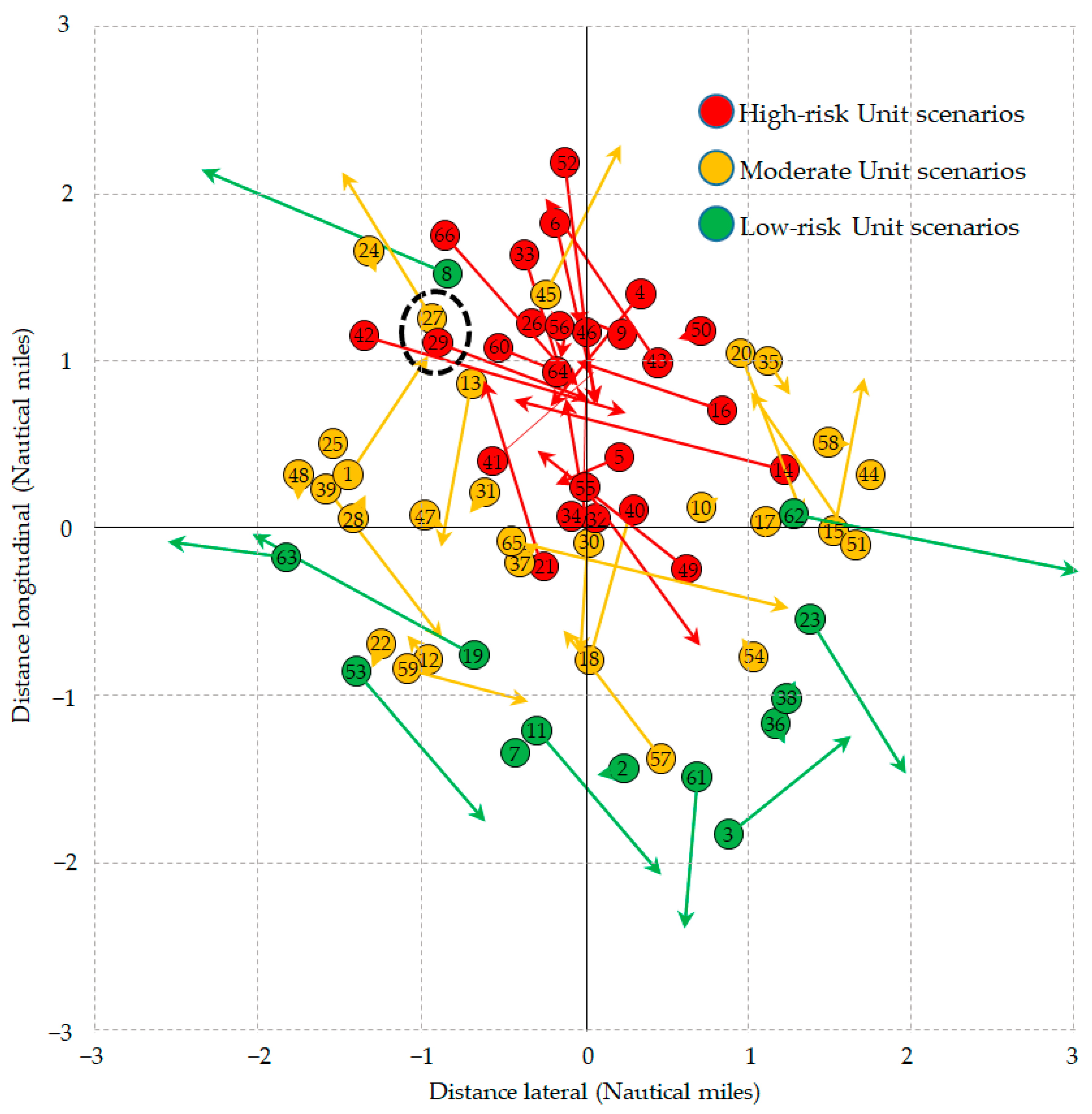
The extracted 1205 CRSs comprise a total of 5110 unit scenarios. Each scenario was clustered based on the relative position, speed, and course of the opposing vessels. The optimal number of clusters was determined to be 66 unit scenario clusters using gap analysis. The 66 distinct unit scenarios identified through this clustering process are depicted in Figure 6. To illustrate the representative characteristics of each cluster, the unit scenarios were visualized using the centroids of the initial and terminal point distributions. Unit scenarios systematically break down various ship encounter situations that are not explicitly defined in the COLREGs, including vessels that pose a collision threat, stationary vessels, and vessels that do not interfere with the navigation of the subject ship. As an example of a categorization, unit Scenarios “29” and “27,” highlighted by the broken line, clearly demonstrate the benefits of unit Scenarios. Both encounter ships in unit scenarios are similarly located about 40 degrees to the port side from the subject ship, but they were categorized differently due to their individual course and speed. To gain a comprehensive understanding of the unit scenarios, which are divided into 66 cluster groups, Figure 6 interprets them into three risk groups based on the distribution of DCPA (distance to closest point of approach). The first group is a high-risk group, which includes vessels approaching the subject ship’s path or so close (DCPA less than 0.5) that there is a high risk of collision. The second group is of moderate risk (DCPA between 0.5 and 2), affecting the decision-making process of the subject ship but not presenting an immediate collision hazard. The third group is a low-risk group (DCPA 2 or more), which includes situations without explicit collision risk where the other ship is either not on the subject ship’s course, stopped, or moving away. However, these groupings are only meant to facilitate a comprehensive understanding of the overall structure of the unit scenario clusters, and it is the cluster numbers, numerically illustrated in Figure 6, that are directly employed as categorical elements in the vectorization of the CRSs in Equation (3).

This equation represents a vector in which the trajectories in Figure 5 are transformed using the categorical labels of the unit scenarios. CRS no. 957 and CRS no. 1099 consist of two and eight encounter ships, respectively, and have been transformed into vectors with two and eight elements, depending on the number of encounters. Each element represents the categorical label of the unit scenario, which means that they have been transformed into an array of vectors containing the relative position, course, and speed of the encounter ships.

$$\begin{gathered} \left(\mathrm{a}\right)\mathrm{CRS}\mathrm{no}.957=\{“6”,“18”\text{}} \\ \left(\mathrm{b}\right)CRSno.1099=\{“7”,“11”,“13”,“15”,“16”,“43”,“51”,“65”\text{}} \end{gathered}$$

(5)

3.3. Graph-Based Model

The similarity between the vectorized CRSs was converted into a similarity matrix using a modified Jaccard similarity measurement. This similarity matrix was used as an input to the graph model, and the total of 1205 CRSs formed a graph network as shown in Figure 7. The dots in this graph represent CRS nodes, which are connected by edges to nodes with similarity to each other. The color of a node indicates its centrality, and it is categorized by increasing centrality, as shown in the color bar on the right. Centrality is an indicator of how many connections a node has to other nodes and is a key factor in assessing the complexity of a CRS node. The thickness of an edge is proportional to the similarity between nodes, with higher similarity represented by thicker edges. The layout of the graph adopts the force-direction method, which means that the higher the similarity between nodes, the more attractive they are, and the lower the similarity, the more repulsive they are. Therefore, the relative positions of nodes can be used to intuitively understand the similarity between them.

Within the graph, nodes can be divided into three main categories based on the centrality and structure of graph network. First, nodes that have relatively less centrality and are colored in the blue range form a peripheral region, called “peripheral nodes.” Second, nodes that are located in the central part of the graph, surrounded by “peripheral nodes,” and are colored from green to yellow are defined as “central nodes.” Finally, nodes with high centrality, which have a strong repulsion to other nodes in the graph and are located in the outer regions of the peripheral nodes, can be classified as “outlier nodes.” The scenarios corresponding to “peripheral nodes,” “central nodes,” and “outlier nodes” are exemplified in Appendix A, Appendix B and Appendix C, though they are not limited to these examples. These scenarios are classified according to the main category of the aforementioned nodes and are presented alongside the normalized centrality (refer to the color bar in Figure 7).

When analyzing this graph from the perspective of scenario development for autonomous ships’ collision avoidance algorithm and enhancing the understanding of CRS, it can be interpreted through three primary dimensions: centrality, frequency, and evolution.

3.3.1. Centrality and Frequency

Centrality is a metric that indicates the extent to which a specific node is connected to others. Therefore, a node’s centrality value indicates the complexity of the corresponding CRS node.

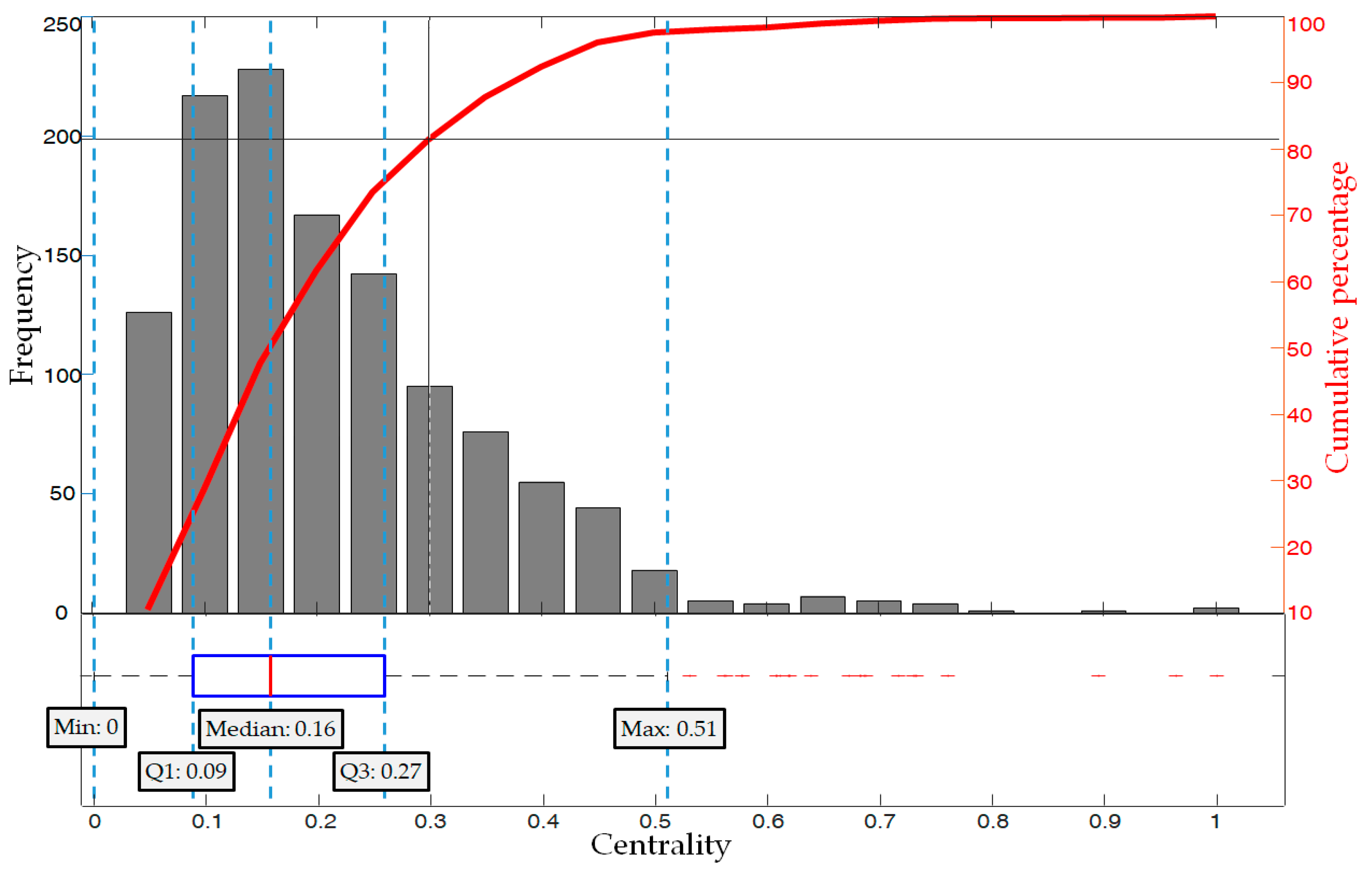
Figure 8 displays the distribution of centrality across nodes via a box plot and bar graph. The median centrality value is 0.16, with an inter-quartile range (IQR) of 0.09 to 0.27. Overall, the distribution demonstrates a bias towards the left side, leaning towards 0 when 0.5 is considered a reference point. Values that are above 1.25 times the IQR in the tail end of the distribution are classified as outliers.

The cumulative percentage also reveals that the majority of the distribution is concentrated in CRSs with low centrality. The left y-axis indicates the frequency of the bar chart, while the right y-axis shows the cumulative percentage of the bar charts. This visualization clarifies the application of the Pareto principle to CRS, which was not easily discernible from the centrality distribution alone. CRS nodes with a centrality value ranging from 0 to 0.3, comprising 30% of the total, occupy approximately 82% of all nodes, and are thus referred to as the “vital few CRSs”. In contrast, the other 70% of nodes with centrality values ranging from 0.3 to 1.0 make up only 18% of the total and are therefore the less-important “Trivial many CRSs”.

3.3.2. Centrality Ascending Evolution

The graph-based model in this research categorizes CRS nodes as peripheral, central, or outlier nodes. Previous analysis has shown that each node is linked to other nodes by edges with similarity values of at least 0, forming a network. Therefore, exploring nodes and edges in the direction of increasing centrality allows for understanding CRS evolution tendencies in actual operational environments. 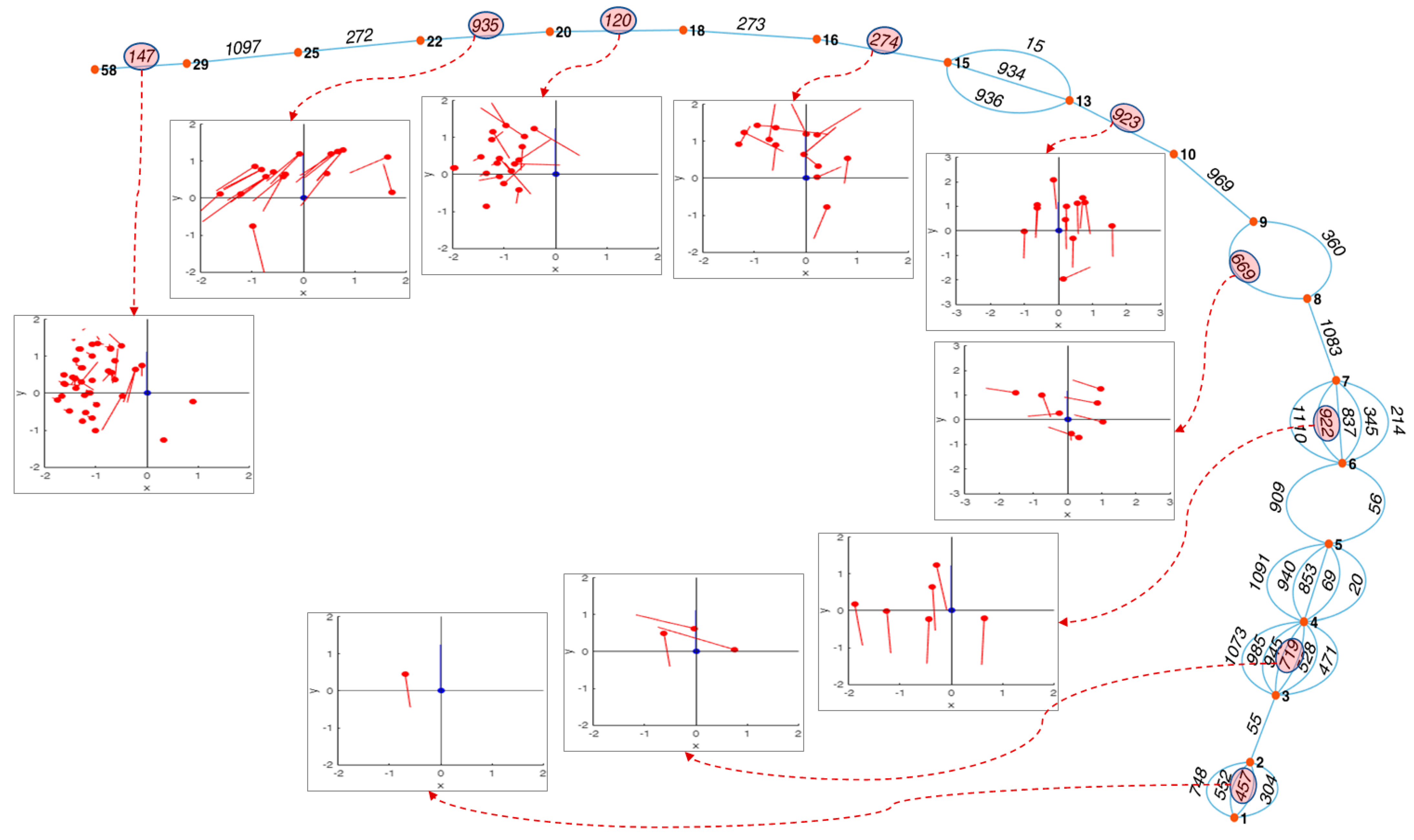Figure 9 illustrates the expansion of the graph in the direction of increasing centrality values, starting from nodes with low centrality values and gradually expanding to connected nodes with higher centrality values.

In Figure 9, the red dots represent the nodes of centrality. The bold text on each node indicates the number of unit scenarios that comprise that CRS, which is the non-normalized value of centrality. Nodes are linked by edges, and the text on these edges indicates the node number of that CRS. The count of edges branching from a centrality node thus represents the count of CRS nodes corresponding to that particular centrality. As shown in the graph, the edges extend from the bottom right to the top left, connecting sequentially from the simplest CRS node to the more complex CRS nodes.

Through the graph, we can clearly see the evolution process of the CRS nodes connected to centrality nodes from (1) to (58) using graph analysis. While each CRS in the sample evolution inherently includes the “port to port” situation, which is frequently encountered during ship navigation, CRS 457 in the lower right represents a one-to-one encounter that is considered relatively simple and ordinary. By examining the examples of ship trajectories presented for each level of centrality, a trend of increasing complexity in the CRS can be observed as centrality increases.

4. Discussion

Through a graph-based analysis, we discerned that CRSs can be categorized into peripheral nodes, central nodes, and outlier nodes, based on the similarity between centrality and CRSs as summarized in

Table 2. Summary of CRS categories based on centrality and graph structure.

CRS Category	Detailed Scenarios
Peripheral nodes	Refer to Appendix A
Central nodes	Refer to Appendix B
Outlier nodes	Refer to Appendix C

. Upon reviewing the scenarios presented in Appendix A, Appendix B and Appendix C, we observe that this graph-based approach enables us to classify and interpret CRSs in a specific manner.

“Peripheral nodes” are closely located, forming a distinct cluster. They form a circular structure, establishing an interconnected network with the nodes within the circular shape. When analyzing these nodes from both a CRS and centrality perspective, their connectivity with other nodes is comparatively lower, suggesting that they can be interpreted as simple and typical CRS scenarios. On the other hand, “central nodes” are nodes that, while being proximate to the peripheral nodes, maintain connections with them. They can be viewed as scenarios with higher complexity than peripheral nodes but can be interpreted as CRSs with routine complexity that are not significantly differentiated from other CRSs. These nodes not only connect with peripheral nodes but also have intrinsic interconnections with other central nodes, indicating a diverse combination of CRS scenarios within a certain similarity range. Meanwhile, the “outlier nodes” in the graph are CRS nodes situated significantly apart from other nodes. Their low similarity with other nodes positions them apart from other nodes. This high centrality indicates that they are unique CRSs with minimal resemblance to other CRSs.

The results of the frequency analysis based on centrality also provided meaningful interpretations. The centrality distribution of all CRS nodes was not distributed normally but skewed toward low centrality. This distribution pattern of centrality indicates that most CRSs represent relatively simple scenarios, while those with a centrality exceeding 0.5 typically embody situations that differ from the norm, indicating their unique nature. This distribution characteristic somewhat aligns with the “Vital few” and “Trivial many” concepts of the Pareto principle. Although it does not perfectly adhere to the 80–20 rule of the Pareto principle, it does confirm that approximately 30% of simple CRSs account for more than 80% of all CRSs, while the remaining 70% of complex and unique CRSs constitute about 20% of the total, showcasing that the concept can indeed be applied to CRSs.

One of the main findings of this study is that we proposed a methodology to systematically explore how simple CRSs evolve into complex CRSs by utilizing centrality ascending evolution. In this study, we sequentially analyzed the development process of CRS centrality, which eventually depicts intricate navigational situations. While the number of possible combinations as centrality increases is vast, the methodology proposed in this study provides a realistic representation of the stepwise evolution of a real-world CRS. This systematic analysis of the actual CRS evolution process is expected to provide a deeper understanding of the collision risk situations that autonomous ships may encounter, as well as an objective basis for the validation of collision avoidance algorithms for autonomous ships.

5. Conclusions

This study presented a scenario development approach for the systematic validation of the collision avoidance system of autonomous ships. The important point is that this approach aims to provide realistic and possible collision risk scenarios based on the understanding of actual collision risk situations. The data-driven approach using AIS data consisted of the preprocessing and extraction of collision risk situations, the vectorization of collision risk situations using unit scenarios, and graph-based modeling using similarity matrix between vectors.

In the graph modeling, we found that collision risk situations can be classified into “peripheral nodes”, “central nodes”, and “outlier nodes” based on the centrality characteristics of the nodes. The peripheral nodes represent simple and frequent collision risk situations, while the central nodes, although complex, represent collision risk situations that are relatively less frequent. In contrast, outlier nodes encapsulate very complex and unique collision risk situations. This centrality characterizes the distribution of collision risk situations according to the Pareto principle, i.e., “vital few” and “trivial many”. The “vital few” represent 30% of the simple collision risk situations, which account for 80% of the total CRSs, while the “trivial many” represent 70% of the complex and unique collision risk situations, which account for 20% of the total CRSs. These findings are expected to be used as a basis for determining the ratio of validation scenarios for autonomous ship collision avoidance systems. One of the key novelties of graph-based modeling of CRSs is the identification of the network structure among CRSs. Centrality ascending evolution was used to visually track how basic encounter situations evolve into complex collision risk situations through the graph network. This can be interpreted as providing the basis for an exhaustive testing of autonomous ships’ collision avoidance system.

The novelty of this research is highlighted by several key differences from previous studies. First, the combination of unit scenarios has been used to implement collision risk situation vectors in graphical form, which represents a unique approach. Second, nodes have been identified in two ways based on graph structure and centrality distribution, adding a unique layer to the investigation. Third, this study introduces a new methodology capable of tracking the evolution from simple collision risk situations to more complex situations, providing a significant value to the field. Finally, since the collision risk situations represented by the classified nodes are based on actual events, they are significant because they provide a new methodology that addresses the reality and scenario diversity issues that have not been addressed in previous collision risk scenario research.

Of course, limitations and future research directions should also be considered. Extending the AIS data collection period to several years is required in order to develop a broader range of possible CRS that autonomous ships may encounter. The application of unit scenarios tends to ignore detailed characteristics by categorizing individual encounters. Future work will focus on improving the granularity of the unit scenario. Furthermore, the feature engineering of unit scenarios demands a method that develops and selects features with more objective grounding. Although the similarity measure used in the vectorization process is well validated, since it is not a traditional method, further supporting research is required. Finally, graph-based modeling is expected to be useful for developing realistic scenarios because it is based on actual CRS. However, due to the open environment of the ocean and the diverse nature of ship traffic, CRS is not limited to historical data. There is always the possibility of new collision risk situations arising that have not been previously characterized. Therefore, the methodology of this study can provide a basic structure for the validation of the collision avoidance system of autonomous ships, but the detailed adjustment of the scenarios will be necessary depending on the purpose and requirements of the validation.

References

- Zhang, L.; Wang, H.; Meng, Q.; Xie, H. Ship accident consequences and contributing factors analyses using ship accident investigation reports. Proc. Inst. Mech. Eng. Part O J. Risk Reliab. 2019, 233, 35–47. [Google Scholar] [CrossRef]
- Bolbot, V.; Theotokatos, G.; Wennersberg, L.A.; Faivre, J.; Vassalos, D.; Boulougouris, E.; Jan Rødseth, Ø.; Andersen, P.; Pauwelyn, A.; Van Coillie, A. A novel risk assessment process: Application to an autonomous inland waterways ship. Proc. Inst. Mech. Eng. Part O J. Risk Reliab. 2023, 237, 436–458. [Google Scholar] [CrossRef]
- Vincent, T.L. Collision Avoidance at Sea, Differential Games and Applications: Proceedings of a Workshop Enschede 1977; Springer: Berlin/Heidelberg, Germany, 2005; pp. 205–221. [Google Scholar]
- Fossen, T.I. Marine Control Systems: Guidance, Navigation and Control of Ships, Rigs and Underwater Vehicles, 3rd ed.; Marine Cybernetics: Trondheim, Norway, 2002. [Google Scholar]
- Peel, D.; Good, N.M. A hidden Markov model approach for determining vessel activity from vessel monitoring system data. Can. J. Fish. Aquat. Sci. 2011, 68, 1252–1264. [Google Scholar] [CrossRef]
- Hu, Q.; Yang, C.; Cheng, H.; Xiao, B. Planned Route Based Negotiation for Collision Avoidance Between Vessels. TransNav Int. J. Mar. Navig. Saf. Sea Transp. 2008, 2, 363–368. [Google Scholar]
- Kearon, J. Computer Programs for Collision Avoidance and Traffic Keeping. In Conference on Mathematical Aspects on Marine Traffic; Academic Press: London, UK, 1977. [Google Scholar]
- Liu, Y.; Shi, C. A fuzzy-neural inference network for ship collision avoidance. In Proceedings of the 2005 International Conference on Machine Learning and Cybernetics, Guangzhou, China, 18–21 August 2005; pp. 4754–4759. [Google Scholar]
- Brcko, T.; Androjna, A.; Srše, J.; Boć, R. Vessel multi-parametric collision avoidance decision model: Fuzzy approach. J. Mar. Sci. Eng. 2021, 9, 49. [Google Scholar] [CrossRef]
- Huang, Y.; Van Gelder, P. Collision risk measure for triggering evasive actions of maritime autonomous surface ships. Saf. Sci. 2020, 127, 104708. [Google Scholar] [CrossRef]
- Mizythras, P.; Pollalis, C.; Boulougouris, E.; Theotokatos, G. A novel decision support methodology for oceangoing vessel collision avoidance. Ocean Eng. 2021, 230, 109004. [Google Scholar] [CrossRef]
- Namgung, H.; Kim, J. Collision risk inference system for maritime autonomous surface ships using COLREGs rules compliant collision avoidance. IEEE Access 2021, 9, 7823–7835. [Google Scholar] [CrossRef]
- Goerlandt, F.; Kujala, P. On the reliability and validity of ship–ship collision risk analysis in light of different perspectives on risk. Saf. Sci. 2014, 62, 348–365. [Google Scholar] [CrossRef]
- Liu, Z.; Wu, Z.; Zheng, Z. A cooperative game approach for assessing the collision risk in multi-vessel encountering. Ocean Eng. 2019, 187, 106175. [Google Scholar] [CrossRef]
- Silveira, P.; Teixeira, A.P.; Figueira, J.R.; Soares, C.G. A multicriteria outranking approach for ship collision risk assessment. Reliab. Eng. Syst. Saf. 2021, 214, 107789. [Google Scholar] [CrossRef]
- Tam, C.; Bucknall, R. Collision risk assessment for ships. J. Mar. Sci. Technol. 2010, 15, 257–270. [Google Scholar] [CrossRef]
- Zhang, W.; Kopca, C.; Tang, J.; Ma, D.; Wang, Y. A systematic approach for collision risk analysis based on AIS data. J. Navig. 2017, 70, 1117–1132. [Google Scholar] [CrossRef]
- Fan, C.; Montewka, J.; Zhang, D. A risk comparison framework for autonomous ships navigation. Reliab. Eng. Syst. Saf. 2022, 226, 108709. [Google Scholar] [CrossRef]
- Guiochet, J.; Machin, M.; Waeselynck, H. Safety-critical advanced robots: A survey. Robot. Auton. Syst. 2017, 94, 43–52. [Google Scholar] [CrossRef]
- Zaitseva, E.; Levashenko, V. Reliability analysis of multi-state system with application of multiple-valued logic. Int. J. Qual. Reliab. Manag. 2017, 34, 862–878. [Google Scholar] [CrossRef]
- Bolbot, V.; Gkerekos, C.; Theotokatos, G.; Boulougouris, E. Automatic traffic scenarios generation for autonomous ships collision avoidance system testing. Ocean Eng. 2022, 254, 111309. [Google Scholar] [CrossRef]
- Alexander, R.; Hawkins, H.R.; Rae, A.J. Situation Coverage—A Coverage Criterion for Testing Autonomous Robots; Technical Report; Department of Computer Science, University of York: Heslington, UK, 2015. [Google Scholar]
- Bolbot, V.; Theotokatos, G.; Bujorianu, L.M.; Boulougouris, E.; Vassalos, D. Vulnerabilities and safety assurance methods in Cyber-Physical Systems: A comprehensive review. Reliab. Eng. Syst. Saf. 2019, 182, 179–193. [Google Scholar] [CrossRef]
- Sørensen, A.J.; Ludvigsen, M. Underwater technology platforms. In Encyclopedia of Maritime and Offshore Engineering; Wiley: Hoboken, NJ, USA, 2017; pp. 1–11. [Google Scholar]
- Torben, T.R.; Glomsrud, J.A.; Pedersen, T.A.; Utne, I.B.; Sørensen, A.J. Automatic simulation-based testing of autonomous ships using Gaussian processes and temporal logic. Proc. Inst. Mech. Eng. Part O J. Risk Reliab. 2023, 237, 293–313. [Google Scholar] [CrossRef]
- Chun, D.; Roh, M.; Lee, H.; Ha, J.; Yu, D. Deep reinforcement learning-based collision avoidance for an autonomous ship. Ocean Eng. 2021, 234, 109216. [Google Scholar] [CrossRef]
- Lazarowska, A. Verification of a deterministic ship’s safe trajectory planning algorithm from different ships’ perspectives and with changing strategies of target ships. TransNav Int. J. Mar. Navig. Saf. Sea Transp. 2021, 15, 623–628. [Google Scholar] [CrossRef]
- Gil, M. A concept of critical safety area applicable for an obstacle-avoidance process for manned and autonomous ships. Reliab. Eng. Syst. Saf. 2021, 214, 107806. [Google Scholar] [CrossRef]
- Szlapczynski, R.; Szlapczynska, J. A ship domain-based model of collision risk for near-miss detection and Collision Alert Systems. Reliab. Eng. Syst. Saf. 2021, 214, 107766. [Google Scholar] [CrossRef]
- Pedersen, T.A.; Glomsrud, J.A.; Ruud, E.; Simonsen, A.; Sandrib, J.; Eriksen, B.H. Towards simulation-based verification of autonomous navigation systems. Saf. Sci. 2020, 129, 104799. [Google Scholar] [CrossRef]
- Porres, I.; Azimi, S.; Lilius, J. Scenario-based testing of a ship collision avoidance system. In Proceedings of the 2020 46th Euromicro Conference on Software Engineering and Advanced Applications (SEAA), Portoroz, Slovenia, 26–28 August 2020; pp. 545–552. [Google Scholar]
- Zhu, F.; Zhou, Z.; Lu, H. Randomly Testing an Autonomous Collision Avoidance System with Real-World Ship Encounter Scenario from AIS Data. J. Mar. Sci. Eng. 2022, 10, 1588. [Google Scholar] [CrossRef]
- Rodriguez, S.I.; de Carvalho, F.d.A. Fuzzy clustering algorithms with distance metric learning and entropy regularization. Appl. Soft Comput. 2021, 113, 107922. [Google Scholar] [CrossRef]
- Saxena, A.; Iyengar, S. Centrality measures in complex networks: A survey. arXiv 2020, arXiv:2011.07190 2020. [Google Scholar]