Optimization Method of Square Hole Measurement Based on Generalized Point Photogrammetry

Abstract

The theory of generalized point photogrammetry extends the traditional point-based photogrammetry to line-based photogrammetry, expanding the application scope of photogrammetry in engineering. In order to solve the problem of accurate positioning between the square rod and the square hole in the current project, the position of the square hole should be accurately measured first. For this purpose, an optimization method of square hole measurement based on generalized point photogrammetry is proposed. This method first uses the traditional photogrammetric method to calculate the initial coordinates of the four points of the square hole and extract the four line segments on the image. The error equation based on generalized photogrammetry is constructed by the constraint conditions between the four spatial points, and the iterative calculation is carried out until the error is less than the threshold or the iteration number is reached. The reliability of the method is verified by numerical simulation experiments and engineering experiments. The experimental results show that the method can effectively improve the measurement accuracy and can rapidly converge. The method has high engineering application value.

1. Introduction

In recent years, with the rapid development of artificial intelligence [1], machine learning [2], cloud computing [3] and other technical fields, photogrammetry has become more and more widely used in engineering [4]. Engineering problems are usually more complex than theoretical problems, and more factors are considered. The traditional point-based photogrammetric method is not enough to solve engineering problems; therefore, the generalized photogrammetric method based on line features is proposed [5]. Generalized photogrammetry originated in the 19th century. After decades of development in theoretical research, it has gradually developed from the classic point-based photogrammetry model to point-line hybrid photogrammetry and generalized point photogrammetry. With the development of big data and the arrival of intelligent photogrammetry, photogrammetry can use more homonymous features to complete the measurement calculation. Intelligent high-precision measurement is urgently needed in engineering. This measurement method not only improves the work efficiency and the safety of measurement, but also greatly reduces the measurement cost. With the performance improvement of computers, sensors, transmission equipment and other hardware [6], a large number of traditional measurement methods [7] will be replaced by intelligent high-precision photogrammetry. Intelligent photogrammetry has many applications in target recognition [8], monitoring [9], unmanned driving [10], three-dimensional modeling [11], precision measurement [12], emergency response [13] and other aspects.

Traditional photogrammetry involves only physical points, such as corners, intersections between lines, centers and so on. The calculation process of traditional photogrammetry is also based on the collinearity of points. However, in engineering, point features [14] are usually ideal features, and it is not easy to extract accurate coordinates of points. There are a lot of line features in engineering [15]. These features exist in the form of straight lines or curves, from which it is easy to extract accurate information. Especially when multiple images are used for calculation in engineering, it is better to use a large number of line features for adjustment. Line features can be divided into straight line features and curve features. There are many straight line features in urban planning and housing surveys [16]. There are many curve features in roads, mountains and rivers [17]. Mathematically, line features and point features can be considered as “points” in a broad sense. From the collinear equation in photogrammetry [4], the coordinates of space points can be regarded as the parameter equation of the line, so that the line features meet the collinear equation. Zheng Shunyi of Wuhan University completed automatic three-dimensional reconstruction of cylinders using the principle of generalized photogrammetry [18], Zhang Yongjun of Wuhan University completed three-dimensional reconstruction of circles and rounded rectangles using the principle of generalized photogrammetry [19], and Kongwei used the principle of generalized photogrammetry to study space intersection and resection [20]. In addition, Zhang Yongjun also proposed generalized photogrammetry based on multi-source remote sensing data of the sky and the ground [21]. The application of general photogrammetry will be more and more extensive.

In recent years, prefabricated bridges have been rapidly promoted in China [22]. At present, the construction site mainly relies on workers to use the total station to complete measurement in the whole process [23]. As a widely used optical instrument, the precision of the total station can meet the construction requirements, but its efficiency is too low. For the on-site construction environment, the field of vision of the total station is too small to measure the coordinates of the points directly. Laser Radar determines the spatial information of targets by receiving reflected signals, but its accuracy cannot meet engineering requirements [24,25,26,27]. Laser scanning has high stability and is suitable for extremely large objects. The generated large point clouds require complex post-processing to complete the extraction of key information. 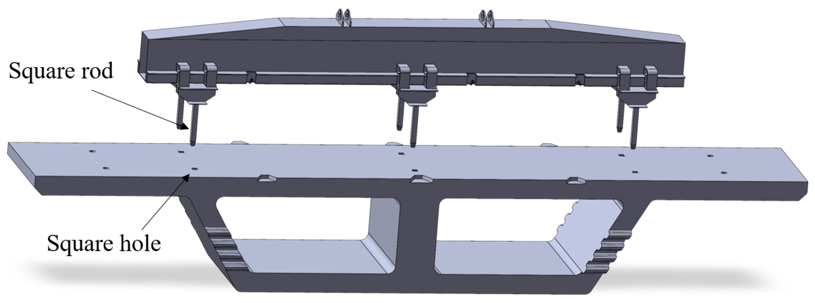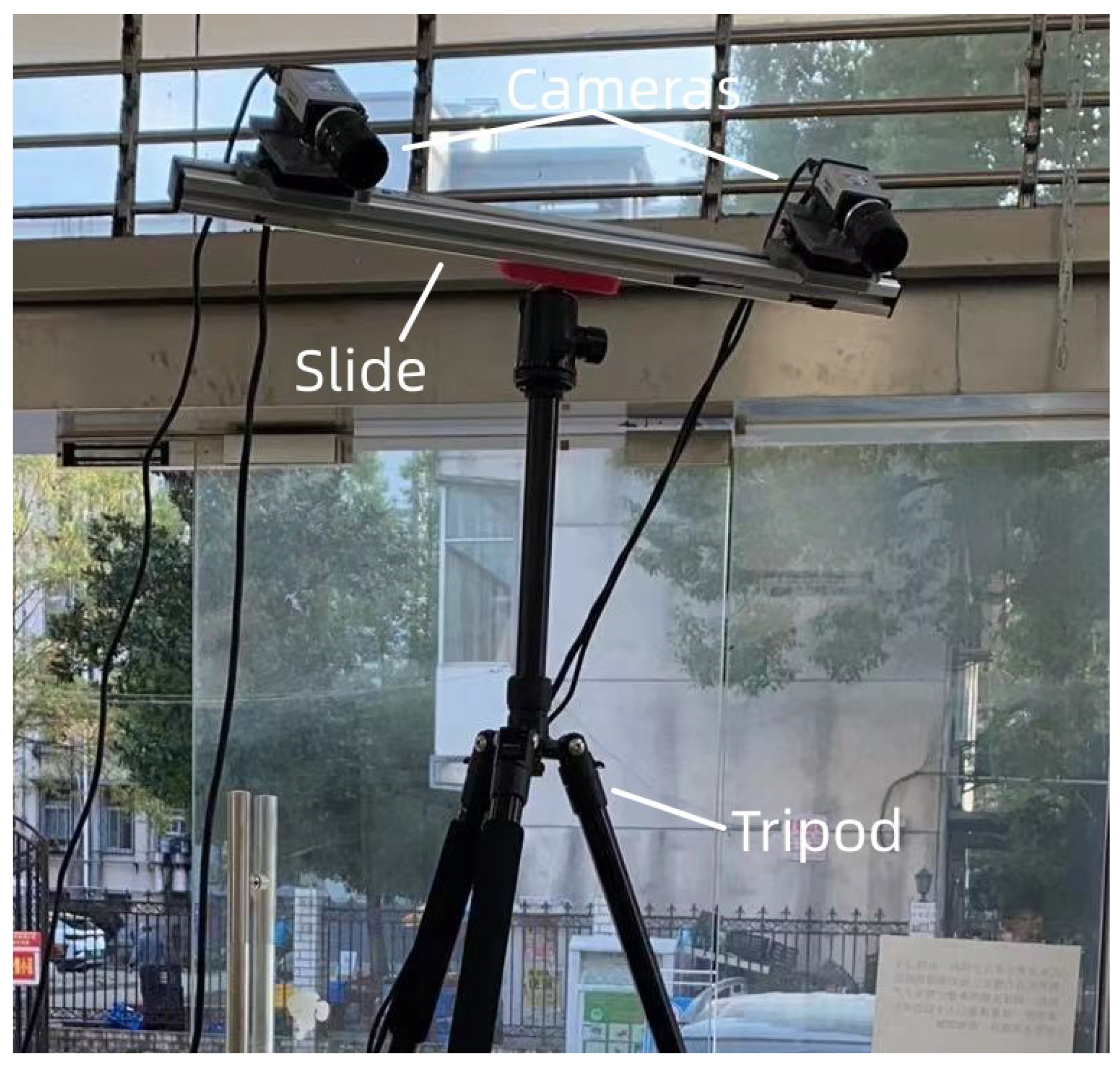Laser scanners are suitable for measuring static objects, but are not suitable for engineering projects that require real-time performance, as they have low efficiency and high cost [28,29]. Therefore, an efficient and fast measurement method is needed to complete the field measurement. In the process of completing the assembly of the segmental beam, it is necessary to lift the segmental beam with the square rod first. In this process, whether the square rod and the square hole can be accurately aligned is very important. As shown in Figure 1, there are six square rods on the lifting tool. After achieving precise alignment of the holes and rods, the control system will insert the six suspension rods into the square holes, and then the lifting tool can lift the beam. The cross sections of the rod and the hole are both square. In order to ensure that the square rod can be placed in the square hole, the side length of the square hole is usually 10 mm longer than the side length of the square rod.

Before aligning the square hole and the square rods, the accurate position of the square hole and the square rod should be calculated to ensure that six square rods are placed in the six square hole simultaneously and then lifted. The above process requires high accuracy. The traditional alignment method mainly relies on manual operation, and the operator needs to manually adjust the position of the square rod to ensure accurate alignment between the hole and the rod. This manual adjustment method has low efficiency and poor safety. Traditional photogrammetry can calculate the space coordinates of key points, but the premise is that the image plane coordinates of the point can be accurately extracted from the image. In engineering environments, the features of points are usually not obvious, and the error in extracting the image plane coordinates of points is usually large. Compared to point features [30,31,32], the extraction of line features [33,34,35,36] should be more stable. Therefore, this paper proposes an optimization method of square hole measurement based on generalized point photogrammetry.

The structure of this article is arranged as follows. Section 2 introduces the mathematical principles of generalized point photogrammetry. On the basis of Section 2, Section 3 introduces the Lagrange multiplier method into general photogrammetry and provides detailed mathematical derivation. On the basis of Section 3, Section 4 has added geometric constraints for square holes and derived optimization methods. On the theoretical basis of the previous chapters, experiments are conducted in Section 6. In order to better verify the robustness and engineering applicability of the algorithm, the experiments are divided into simulation experiments and engineering experiments. This article has the following innovative points. A generalized point photogrammetric mathematical model based on the Lagrange multiplier method is proposed. A square hole optimization method based on constraint conditions is proposed. This article combines image processing technology with photogrammetry technology and is used to solve practical engineering problems.

2. Mathematical Model of Generalized Point Photogrammetry

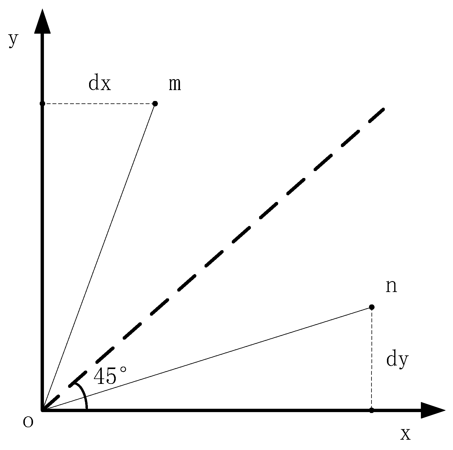
The collinearity equation is the core of photogrammetry, and the collinearity of points is the basis of photogrammetric solution. As shown in Figure 2, point m and point n represent the projection point of the space point on the image. The angle between the straight line segment where point m is located and the x-axis is greater than 45 degrees, and the angle between the straight line segment where point n is located and the x-axis is less than 45 degrees. Point m is closer to the y-axis, and point n is closer to the x-axis.

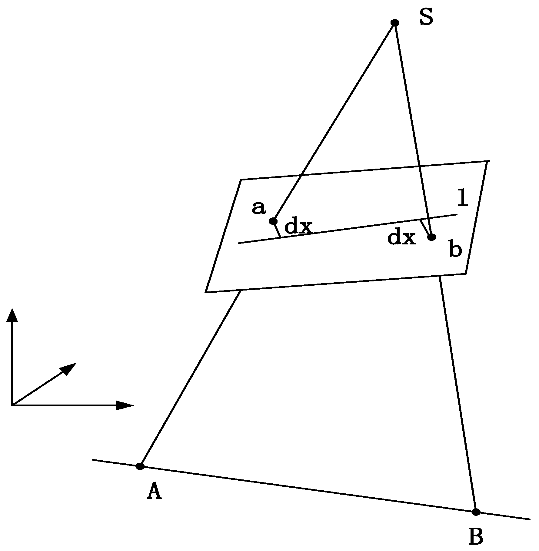
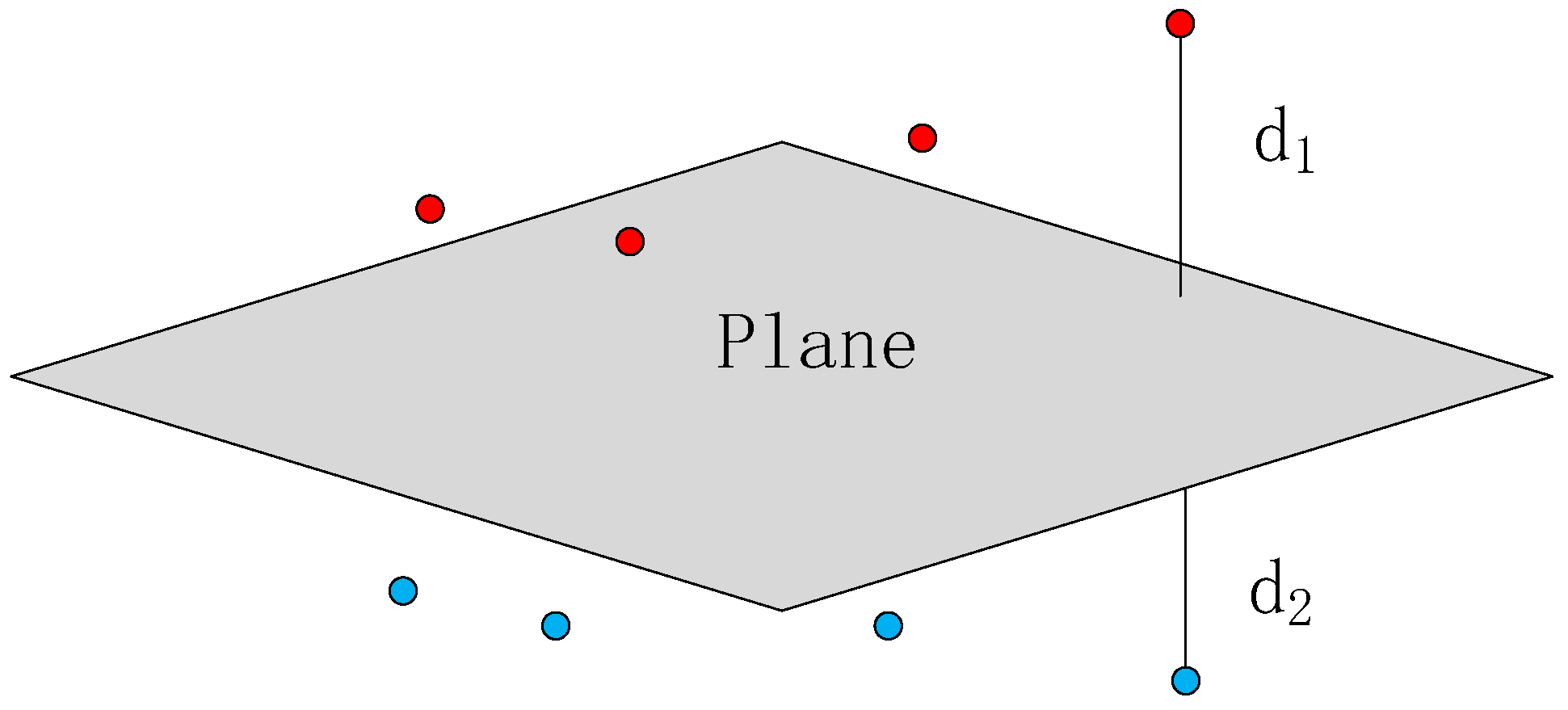
As shown in Figure 3, S is the projection center, and the projection of spatial points A and B on the image are a and b. The image coordinates of a and b are calculated through photogrammetry, and the line l is the projection of the line $AB$ on the image. Due to errors, a and b are usually not on the straight line l. The generalized point photogrammetric model based on straight lines only needs an error equation in one direction. The adjustment condition is that the distance dx (or dy) from the projection of the space point on the image to the ideal image point is the smallest.

When the angle between the direction of the straight line segment on the image and the x-axis is greater than 45 degrees, the observation equation in the x-direction is listed. When the angle between the direction of the straight line segment on the image and the y axis is less than 45 degrees, the observation equation in the y direction is listed. The mathematical expression of the observation equation is as follows.

$$x-x_0=-f\frac{a_1\left(X-X_s\right)+b_1\left(Y-Y_s\right)+c_1\left(Z-Z_s\right)}{a_3\left(X-X_s\right)+b_3\left(Y-Y_s\right)+c_3\left(Z-Z_s\right)},\left|\theta \right|\ge {45}^{°}$$

(1)

$$y-y_0=-f\frac{a_2\left(X-X_s\right)+b_2\left(Y-Y_s\right)+c_2\left(Z-Z_s\right)}{a_3\left(X-X_s\right)+b_3\left(Y-Y_s\right)+c_3\left(Z-Z_s\right)},\left|\theta \right|<{45}^{°}$$

(2)

where,

$$\begin{array}{c}{a}_1=cos\phi cos\kappa \hfill \\ a_2=-cos\phi sin\kappa \hfill \\ a_3=-sin\phi \hfill \\ b_1=cos\omega sin\kappa -sin\omega sin\phi cos\kappa \hfill \\ b_2=cos\omega cos\kappa +sin\omega sin\phi sin\kappa \hfill \\ b_3=-sin\omega cos\phi \hfill \\ c_1=sin\omega sin\kappa +cos\omega sin\phi cos\kappa \hfill \\ c_2=sin\omega cos\kappa -cos\omega sin\phi sin\kappa \hfill \\ c_3=cos\omega cos\phi \hfill \end{array}$$

(3)

where, x and y are the image plane coordinates of the image point; $x_0$, $y_0$ and f are elements of interior orientation; $X_S$, $Y_S$ and $Z_S$ are the elements of exterior orientation; X, Y and Z are the object space coordinates of the object point; $a_i$, $b_i$ and $c_i$ (i = 1, 2, 3) are the directional cosines of three angular elements.

For line features in space, when two points ($X_1$, $Y_1$, $Z_1$), ($X_2$, $Y_2$, $Z_2$) on the line are known, the equation expression is as follows.

$$\frac{X-X_1}{X_2-X_1}=\frac{Y-Y_1}{Y_2-Y_1}=\frac{Z-Z_1}{Z_2-Z_1}=t$$

(4)

Substitute the above linear equation into collinear equation.

$$x-x_0=-f\frac{\begin{array}{c}{a}_1\left((X_2-X_1)t+X_1-X_S\right)+b_1\left((Y_2-Y_1)t+Y_1-Y_S\right)\hfill \\ +c_1\left((Z_2-Z_1)t+Z_1-Z_S\right)\hfill \end{array}}{\begin{array}{c}{a}_3\left((X_2-X_1)t+X_1-X_S\right)+b_3\left((Y_2-Y_1)t+Y_1-Y_S\right)\hfill \\ +c_3\left((Z_2-Z_1)t+Z_1-Z_S\right)\hfill \end{array}},\left|\theta \right|\ge {45}^{°}$$

(5)

$$y-y_0=-f\frac{\begin{array}{c}{a}_2\left((X_2-X_1)t+X_1-X_S\right)+b_2\left((Y_2-Y_1)t+Y_1-Y_S\right)\hfill \\ +c_2\left((Z_2-Z_1)t+Z_1-Z_S\right)\hfill \end{array}}{\begin{array}{c}{a}_3\left((X_2-X_1)t+X_1-X_S\right)+b_3\left((Y_2-Y_1)t+Y_1-Y_S\right)\hfill \\ +c_3\left((Z_2-Z_1)t+Z_1-Z_S\right)\hfill \end{array}},\left|\theta \right|<{45}^{°}$$

(6)

To solve each parameter in the linear equation by using the generalized point photogrammetry principle, the initial value of two points on the spatial linear equation must be known first. Assuming the coordinates of the observation points are ($x_1$, $y_1$), when the angle between the straight line and the x-axis direction is greater than 45 degrees, the observation equation in the x-direction is established. The value of parameter t can be obtained from the collinear equation in the y direction, and the expression is as follows.

$$t=-\frac{\begin{array}{c}f(a_2(X_1-X_s)+b_2(Y_1-Y_s)+c_2(Z_1-Z_s))\hfill \\ +y_1(a_3(X_1-X_s)+b_3(Y_1-Y_s)+c_3(Z_1-Z_s))\hfill \end{array}}{\begin{array}{c}f(a_2(X_2-X_1)+b_2(Y_2-Y_1)+c_2(Z_2-Z_1))\hfill \\ +y_1(a_3(X_2-X_1)+b_3(Y_2-Y_1)+c_3(Z_2-Z_1))\hfill \end{array}}$$

(7)

On the premise of solving t, the error equation of x direction can be listed.

$$v_x=x_1-x_0+f\frac{\begin{array}{c}{a}_1\left((X_2-X_1)t+X_1-X_s\right)+b_1\left((Y_2-Y_1)t+Y_1-Y_s\right)\hfill \\ +c_1\left((Z_2-Z_1)t+Z_1-Z_s\right)\hfill \end{array}}{\begin{array}{c}{a}_3\left((X_2-X_1)t+X_1-X_s\right)+b_3\left((Y_2-Y_1)t+Y_1-Y_s\right)\hfill \\ +c_3\left((Z_2-Z_1)t+Z_1-Z_s\right)\hfill \end{array}}$$

(8)

If the error equation is linearized, the following formula is obtained.

$$x_1=\left(x_1\right)+\frac{\partial x_1}{\partial X_1}d{X}_1+\frac{\partial x_1}{\partial Y_1}d{Y}_1+\frac{\partial x_1}{\partial Z_1}d{Z}_1+\frac{\partial x_1}{\partial X_2}d{X}_2+\frac{\partial x_1}{\partial Y_2}d{Y}_2+\frac{\partial x_1}{\partial Z_2}d{Z}_2$$

(9)

where, ($x_1$) is the approximate value of the result of the previous iteration. The calculation formulas of each coefficient are as follows.

$$\begin{array}{c}\frac{\partial x_1}{\partial X_1}=-(1-t)a_{11},\frac{\partial x_1}{\partial Y_1}=-(1-t)a_{12},\frac{\partial x_1}{\partial Z_1}=-(1-t)a_{13}\\ \frac{\partial x_1}{\partial X_2}=-t{a}_{11},\frac{\partial x_1}{\partial Y_2}=-t{a}_{12},\frac{\partial x_1}{\partial Z_2}=-t{a}_{13}\end{array}$$

(10)

$$\begin{array}{c}{a}_{11}=\frac{1}{\overline{Z}}[a_{1}f+a_3(x-x_0)]\\ a_{12}=\frac{1}{\overline{Z}}[b_{1}f+b_3(x-x_0)]\\ a_{13}=\frac{1}{\overline{Z}}[c_{1}f+c_3(x-x_0)]\end{array}$$

(11)

where,

$$\overline{Z}=a_3(X-X_S)+b_3(Y-Y_S)+c_3(Z-Z_S)$$

(12)

When the angle between the straight line and the x-axis direction is less than 45 degrees, the observation equation in the y-direction is established. The value of parameter t can be obtained from the collinear equation in the x direction, and the expression is as follows.

$$t=-\frac{\begin{array}{c}f(a_1(X_1-X_s)+b_1(Y_1-Y_s)+c_1(Z_1-Z_s))\hfill \\ +x_1(a_3(X_1-X_s)+b_3(Y_1-Y_s)+c_3(Z_1-Z_s))\hfill \end{array}}{\begin{array}{c}f(a_1(X_2-X_1)+b_1(Y_2-Y_1)+c_1(Z_2-Z_1))\hfill \\ +x_1(a_3(X_2-X_1)+b_3(Y_2-Y_1)+c_3(Z_2-Z_1))\hfill \end{array}}$$

(13)

On the premise of finding t, the error equation of y direction can be listed.

$$v_y=y_1-y_0+f\frac{\begin{array}{c}{a}_2\left((X_2-X_1)t+X_1-X_s\right)+b_2\left((Y_2-Y_1)t+Y_1-Y_s\right)\hfill \\ +c_2\left((Z_2-Z_1)t+Z_1-Z_s\right)\hfill \end{array}}{\begin{array}{c}{a}_3\left((X_2-X_1)t+X_1-X_s\right)+b_3\left((Y_2-Y_1)t+Y_1-Y_s\right)\hfill \\ +c_3\left((Z_2-Z_1)t+Z_1-Z_s\right)\hfill \end{array}}$$

(14)

The following formula is used to linearize the error equation.

$$y_1=\left(y_1\right)+\frac{\partial y_1}{\partial X_1}d{X}_1+\frac{\partial y_1}{\partial Y_1}d{Y}_1+\frac{\partial y_1}{\partial Z_1}d{Z}_1+\frac{\partial y_1}{\partial X_2}d{X}_2+\frac{\partial y_1}{\partial Y_2}d{Y}_2+\frac{\partial y_1}{\partial Z_2}d{Z}_2$$

(15)

where, (y1) is the approximate value of the result of the previous iteration. The calculation formulas of each coefficient are as follows.

$$\begin{array}{c}\frac{\partial y_1}{\partial X_1}=-(1-t)a_{21},\frac{\partial y_1}{\partial Y_1}=-(1-t)a_{22},\frac{\partial y_1}{\partial Z_1}=-(1-t)a_{23}\\ \frac{\partial y_1}{\partial X_2}=-t{a}_{21},\frac{\partial y_1}{\partial Y_2}=-t{a}_{22},\frac{\partial y_1}{\partial Z_2}=-t{a}_{23}\end{array}$$

(16)

$$\begin{array}{c}{a}_{21}=\frac{1}{\overline{Z}}[a_{2}f+a_3(y-y_0)]\\ a_{22}=\frac{1}{\overline{Z}}[b_{2}f+b_3(y-y_0)]\\ a_{23}=\frac{1}{\overline{Z}}[c_{2}f+c_3(y-y_0)]\end{array}$$

(17)

The accurate values of the coordinates of two points ($X_1$, $Y_1$, $Z_1$), ($X_2$, $Y_2$, $Z_2$) on the straight line can be obtained by solving the error equation iteratively.

3. Generalized Point Photogrammetry Based on Lagrange Multiplier Method

When using the principle of photogrammetry to calculate the coordinates of space points, there are usually redundant observations. When using multiple observations for adjustment, it is necessary to build an adjustment equation group [37]. The error equation is shown below.

$$V=BX-l$$

(18)

where, V is the error, V is also an explicit function of X, B is the coefficient matrix, X is the correction of unknown number, and l is the difference between the measured value and the observed value. The constraint equation is as follows.

$$CX+W_X=0$$

(19)

where C is coefficient matrix, $W_x$ is a constant. From the above error Equation (18) and constraint Equation (19), the Lagrange multiplier method can be used to construct the following equation for solution.

$$F\left(X\right)=VPV+2\lambda (CX+W_X)$$

(20)

The above Formula (20) has the following formula for the derivative of X.

$$V^{T}PB+{\lambda }^{T}C=0$$

(21)

After transposing the above Formula (21), there is the following formula.

$$B^{T}PV+C^T\lambda =0$$

(22)

The following formula can be obtained by substituting Formula (18) into Formula (22).

$$B^{T}PBX+C^T\lambda -B^{T}Pl=0$$

(23)

The following formula can be obtained from the above formula.

$$N_{B}X+C^T\lambda -W=0$$

(24)

where, $N_B=B^{T}PB,W=B^{T}Pl$.

The following formula can be obtained by multiplying $C{N_B}^{-1}$ left by Formula (24). The following formula can be obtained by combining the above Formulas (19) and (24).

$$C{N_B}^{-1}{C}^T\lambda -C{N_B}^{-1}W+W_X=0$$

(25)

The following formula can be obtained from the above formula.

$$\lambda =C{N_B}^{-1}{C}^T(C{N_B}^{-1}W+W_X)$$

(26)

The following formula can be obtained by substituting the above formula into (24).

$$X=({N_B}^{-1}-{N_B}^{-1}{C}^T{N}_{C}C{N_B}^{-1})W-{N_B}^{-1}{C}^T{N_C}^{-1}{W}_X$$

(27)

where, $N_C=C{N_B}^{-1}{C}^T$.

4. Mathematical Model of Square Hole Measurement Based on Constraint Conditions

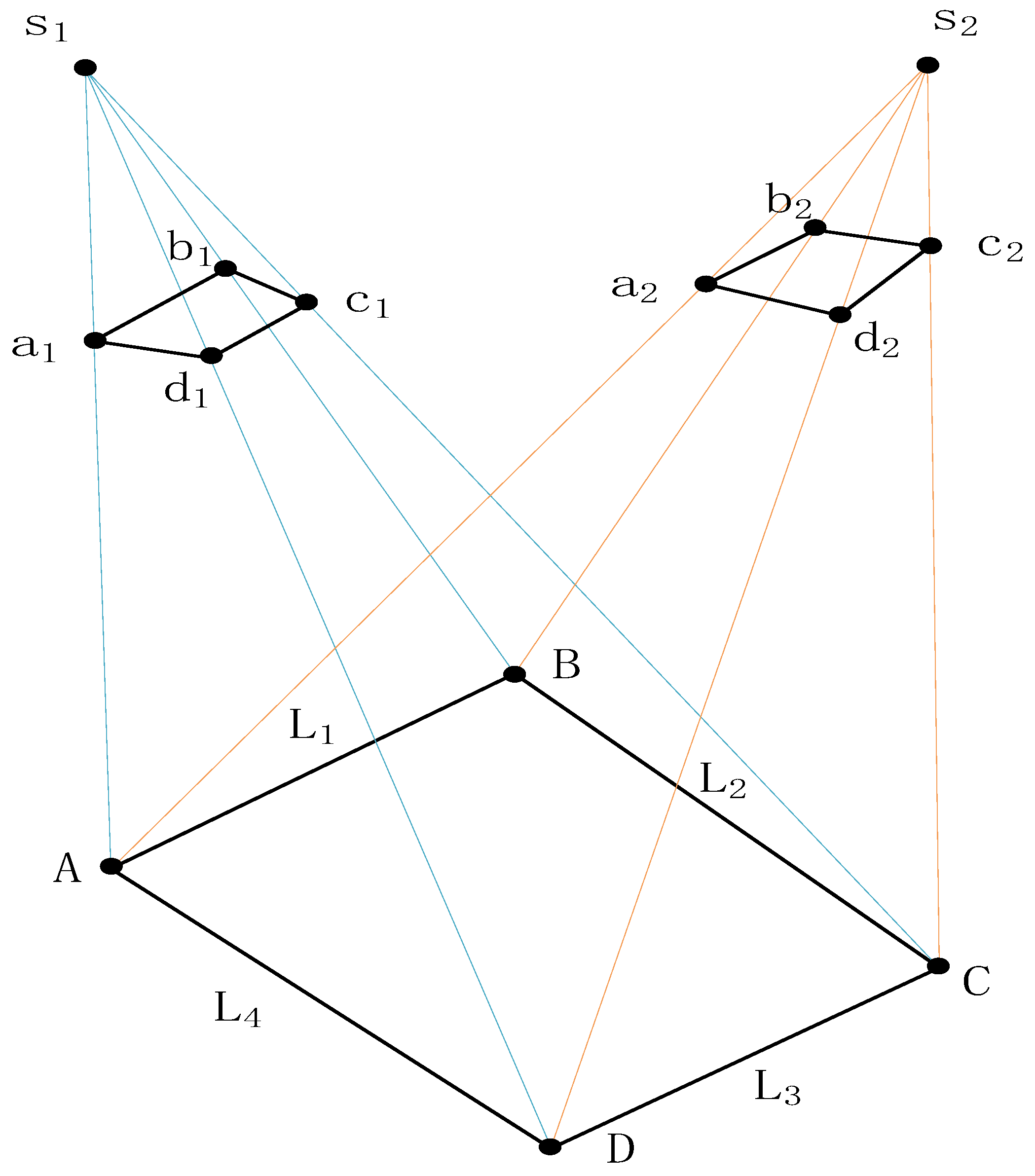
As shown in Figure 4, it is a schematic diagram of a space square hole. Under ideal conditions, the four points A, B, C and D are in the same plane and form a plane square. The spatial coordinates of the four points are $(X_1,Y_1,Z_1)$, $(X_2,Y_2,Z_2)$, $(X_3,Y_3,Z_3)$ and $(X_4,Y_4,Z_4)$. Line segment $L_1$ is determined by point A and B, line segment $L_2$ is determined by point B and C, line segment $L_3$ is determined by point C and D, and line segment $L_4$ is determined by point A and D. $S_1$ and $S_2$ are the projection centers of the two images. Points $a_1$, $b_1$, $c_1$ and $d_1$ are the projection of the spatial points A, B, C and D on the first image. Points $a_2$, $b_2$, $c_2$ and $d_2$ are the projection of the spatial points on the second image.

Since the four points form a plane square, the following constraints need to be set.

$$\begin{array}{c}\overrightarrow{L_1}\perp \overrightarrow{L_2}\hfill \\ \overrightarrow{L_1}\perp \overrightarrow{L_4}\hfill \\ \overrightarrow{L_2}\perp \overrightarrow{L_3}\hfill \\ \overrightarrow{L_3}\perp \overrightarrow{L_4}\hfill \\ \overrightarrow{|L_1}|\perp |\overrightarrow{L_2}|=m\hfill \end{array}$$

(28)

where, m is the square side length.

The following formula can be obtained from the constraint conditions.

$$\begin{array}{c}(X_2-X_1,Y_2-Y_1,Z_2-Z_1)(X_3-X_2,Y_3-Y_2,Z_3-Z_2)=0\hfill \\ (X_2-X_1,Y_2-Y_1,Z_2-Z_1)(X_4-X_1,Y_4-Y_1,Z_4-Z_1)=0\hfill \\ (X_3-X_4,Y_3-Y_4,Z_3-Z_4)(X_3-X_2,Y_3-Y_2,Z_3-Z_2)=0\hfill \\ (X_3-X_4,Y_3-Y_4,Z_3-Z_4)(X_4-X_1,Y_4-Y_1,Z_4-Z_1)=0\hfill \\ {(X_2-X_1)}^2+{(Y_2-Y_1)}^2+{(Z_2-Z_1)}^2-m^2=0\hfill \\ {(X_2-X_3)}^2+{(Y_2-Y_3)}^2+{(Z_2-Z_3)}^2-m^2=0\hfill \end{array}$$

(29)

For the first constraint, the following equation can be obtained after the formula is functioned.

$$\begin{array}{c}{F}_1^K=F_1^0+\frac{\partial F_1}{X_1}d{X}_1+\frac{\partial F_1}{X_2}d{X}_2+\frac{\partial F_1}{X_3}d{X}_3+\frac{\partial F_1}{X_4}d{X}_4\hfill \\ +\frac{\partial F_1}{Y_1}d{Y}_1+\frac{\partial F_1}{Y_2}d{Y}_2+\frac{\partial F_1}{Y_3}d{Y}_3+\frac{\partial F_1}{Y_4}d{Y}_4\hfill \\ +\frac{\partial F_1}{Z_1}d{Z}_1+\frac{\partial F_1}{Z_2}d{Z}_2+\frac{\partial F_1}{Z_3}d{Z}_3+\frac{\partial F_1}{Z_4}d{Z}_4\hfill \end{array}$$

(30)

where,

$$\begin{array}{c}\frac{\partial F_1}{\partial X_1}=X_2-X_3,\frac{\partial F_1}{\partial X_2}=-2X_2+X_3+X_1,\frac{\partial F_1}{\partial X_3}=X_2-X_1,\frac{\partial F_1}{\partial X_4}=0\\ \frac{\partial F_1}{\partial Y_1}=Y_2-Y_3,\frac{\partial F_1}{\partial Y_2}=-2Y_2+Y_3+Y_1,\frac{\partial F_1}{\partial Y_3}=Y_2-Y_1,\frac{\partial F_1}{\partial Y_4}=0\\ \frac{\partial F_1}{\partial Z_1}=Z_2-Z_3,\frac{\partial F_1}{\partial Z_2}=-2Z_2+Z_3+Z_1,\frac{\partial F_1}{\partial Z_3}=Z_2-Z_1,\frac{\partial F_1}{\partial Z_4}=0\end{array}$$

(31)

In the same way, linearization formulas for other constraints can be obtained. After the error equations of all observation points are established, iterative calculation can be carried out to obtain the precise spatial coordinates of the four points of the square hole.

5. Experiments

5.1. Simulation Experiment

In order to verify the reliability of the square hole measurement method based on constraint conditions, the simulation data are used for theoretical verification, and the external orientation elements are set, as seen in

Table 1. Camera extrinsic parameters.

Images	$\mathit{\phi }$	$\mathit{\omega }$	$\mathit{\kappa }$	${\mathit{X}}_{\mathit{S}}$	${\mathit{Y}}_{\mathit{S}}$	${\mathit{Z}}_{\mathit{S}}$
First image	0	0	1813	0	0	0.2
Second image	200	200	1818	0	0	0.1

. The simulation experiment completed several groups of experiments with Gaussian error, camera focal length and square hole side length as variables. The coordinates extracted by image processing are considered as the true values of coordinates, and the coordinates calculated by traditional photogrammetric methods are considered as the initial values of the coordinates. The schematic diagram is shown in Figure 4.

There are eight groups in the tests, and the parameters set are shown in

Table 2. Experimental parameters.

Test	Gaussian Error ($\mathit{\mu }$, $\mathit{\sigma }$)	Focal Lengths	Length of Square Hole
1	(0, 1)	(20, 20)	100
2	(0, 1)	(20, 20)	150
3	(0, 1)	(30, 30)	100
4	(0, 1)	(30, 30)	150
5	(2, 5)	(20, 20)	100
6	(2, 5)	(20, 20)	150
7	(2, 5)	(30, 30)	100
8	(2, 5)	(30, 30)	150

.

The true coordinates of the eight tests are shown in

Table 3. True spatial coordinates.

Test	(${\mathit{X}}_1,{\mathit{Y}}_1,{\mathit{Z}}_1$)	(${\mathit{X}}_2,{\mathit{Y}}_2,{\mathit{Z}}_2$)	(${\mathit{X}}_3,{\mathit{Y}}_3,{\mathit{Z}}_3$)	(${\mathit{X}}_4,{\mathit{Y}}_4,{\mathit{Z}}_4$)
1	(0, 100, 100)	(100, 100, 100)	(100, 0, 100)	(0, 0, 100)
2	(0, 150, 100)	(150, 150, 100)	(150, 0, 100)	(0, 0, 100)
3	(0, 100, 100)	(100, 100, 100)	(100, 0, 100)	(0, 0, 100)
4	(0, 150, 100)	(150, 150, 100)	(150, 0, 100)	(0, 0, 100)
5	(0, 100, 100)	(100, 100, 100)	(100, 0, 100)	(0, 0, 100)
6	(0, 150, 100)	(150, 150, 100)	(150, 0, 100)	(0, 0, 100)
7	(0, 100, 100)	(100, 100, 100)	(100, 0, 100)	(0, 0, 100)
8	(0, 150, 100)	(150, 150, 100)	(150, 0, 100)	(0, 0, 100)

.

Corresponding to the Gaussian error in the above table, the initial coordinates of spatial points of eight experiments are shown as

Table 4. Initial Spatial coordinates.

Test	(${\mathit{X}}_1,{\mathit{Y}}_1,{\mathit{Z}}_1$)	(${\mathit{X}}_2,{\mathit{Y}}_2,{\mathit{Z}}_2$)	(${\mathit{X}}_3,{\mathit{Y}}_3,{\mathit{Z}}_3$)	(${\mathit{X}}_4,{\mathit{Y}}_4,{\mathit{Z}}_4$)
1	(0.54, 100.32, 103.58)	(101.83, 98.69, 102.77)	(97.74, 0.43, 98.65)	(0.86, 0.34, 103.03)
2	(3.62, 151.72, 103.50)	(151.86, 155.33, 99.30)	(153.60, 5.15, 103.60)	(1.54, 5.17, 105.65)
3	(0.54, 100.32, 103.58)	(101.83, 98.69, 102.77)	(97.74, 0.43, 98.65)	(0.86, 0.34, 103.03)
4	(3.62, 151.72, 103.50)	(151.86, 155.33, 99.30)	(153.60, 5.15, 103.60)	(1.54, 5.17, 105.65)
5	(3.62, 101.72, 103.50)	(101.86, 105.33, 99.30)	(103.60, 5.15, 103.60)	(1.54, 5.17, 105.65)
6	(3.62, 151.72, 103.50)	(151.86, 155.33, 99.30)	(153.60, 5.15, 103.60)	(1.54, 5.17, 105.65)
7	(3.62, 101.72, 103.50)	(101.86, 105.33, 99.30)	(103.60, 5.15, 103.60)	(1.54, 5.17, 105.65)
8	(3.62, 151.72, 103.50)	(151.86, 155.33, 99.30)	(153.60, 5.15, 103.60)	(1.54, 5.17, 105.65)

.

The results of eight experiments are shown in

Table 5. Results of the experiments.

Test	Iterations	(${\mathit{X}}_1,{\mathit{Y}}_1,{\mathit{Z}}_1$)	(${\mathit{X}}_2,{\mathit{Y}}_2,{\mathit{Z}}_2$)	(${\mathit{X}}_3,{\mathit{Y}}_3,{\mathit{Z}}_3$)	(${\mathit{X}}_4,{\mathit{Y}}_4,{\mathit{Z}}_4$)
1	22	(0, 100, 100)	(100, 100, 100)	(100, 0, 100)	(0, 0, 100)
2	23	(0, 150, 100)	(150, 150, 100)	(150, 0, 100)	(0, 0, 100)
3	22	(0, 100, 100)	(100, 100, 100)	(100, 0, 100)	(0, 0, 100)
4	23	(0, 150, 100)	(150, 150, 100)	(150, 0, 100)	(0, 0, 100)
5	23	(0, 100, 100)	(100, 100, 100)	(100, 0, 100)	(0, 0, 100)
6	23	(0, 150, 100)	(150, 150, 100)	(150, 0, 100)	(0, 0, 100)
7	23	(0, 100, 100)	(100, 100, 100)	(100, 0, 100)	(0, 0, 100)
8	23	(0, 150, 100)	(150, 150, 100)	(150, 0, 100)	(0, 0, 100)

.

It can be seen from Table that when there are different degrees of errors between the initial value and the true value of coordinates, the eight groups of experiments can quickly converge to an accurate value with fewer iterative steps. Whether the focal length is changed or the side length of the square hole is changed, the convergence results are not affected.

5.2. Engineering Experiment

5.2.1. Engineering Experiment Process

As shown in Figure 5, iRAYPLE’s industrial camera is used to build a visual measurement model in the experiment. Both cameras can move on the slide or adjust the angle on the slide. The slide and tripod are connected by ball joints, and the angle can also be adjusted. The tripod can be adjusted in height by telescoping. The camera is connected to the computer through a control cable, and the camera is controlled to take photos through the computer.

As shown in Figure 6, in order to meet the needs of engineering experiments, a physical model of the hole and rod was constructed by simulating the alignment between the rod and the hole. The cross-section of the upper part of the rod is a square with a side length of 120 mm. Below the rod is a square hole with a side length of 130 mm.

The experimental process is shown in Figure 7. After completing camera calibration, traditional photogrammetric methods are used to calculate the initial coordinates of the four corner points of the hole, and then the initial coordinates are substituted into the generalized point iterative adjustment mathematical model to obtain the accurate coordinates of four corner points.

5.2.2. Results and Analysis of Engineering Experiments

The camera resolution is 4096 × 3000, with a pixel size of 3.45 μm. The camera’s intrinsic parameters are shown in

Table 6. Camera intrinsic parameters.

	f (mm)	$\mathbf{\Delta }\mathit{x}$ (mm)	$\mathbf{\Delta }\mathit{y}$ (mm)	${\mathit{k}}_1$	${\mathit{k}}_2$
Camera 1	34.58	−0.1833	0.0761	−0.0785	1.5814
Camera 2	34.45	−0.0187	−0.1622	−0.0058	0.2803

. f represents the focal length, $\Delta$x and $\Delta$y represent the offset of the image principal point, and $k_1$ and $k_2$ are the radial distortion parameters.

The extrinsic parameters of the cameras are shown in

Table 7. Exterior orientation elements of two images.

	$\mathit{\phi }$ (rad)	$\mathit{\omega }$ (rad)	$\mathit{\kappa }$ (rad)	${\mathit{X}}_{\mathit{S}}$ (mm)	${\mathit{Y}}_{\mathit{S}}$ (mm)	${\mathit{Z}}_{\mathit{S}}$ (mm)
First image	232.3033	−221.4771	105.0735	1.3910	2.6595	2.6192
Second image	−5.6175	−8.4404	109.0247	3.1404	0.0154	3.2693

.

The image plane coordinates of the four corner points of the square hole are shown in

Table 8. Image plane coordinates of the four corner points.

Points	First Image	Second Image
Corner 1	(−7.1382, 22.1317)	(−20.8293, 399.0914)
Corner 2	(−18.0413, 39.2535)	(−324.7541, 410.0443)
Corner 3	(−12.3197, 32.7147)	(−289.9472, 85.0483)
Corner 4	(−1.3404, 14.8592)	(−50.1016, 43.9029)

.

The initial spatial coordinates of the four corner points of the square hole calculated through traditional photogrammetry are shown in

Table 9. Initial spatial coordinates of the four corner points.

Points	X (mm)	Y (mm)	Z (mm)
Corner 1	1.5321	133.2612	105.0325
Corner 2	134.5622	135.6421	103.5761
Corner 3	132.5415	3.5725	102.0712
Corner 4	3.0754	−1.7523	102.1672

.

The results of straight line fitting at the edge of the square hole are shown in Figure 8.

The accurate spatial coordinates of the four corner points of the hole calculated through the generalized point adjustment mathematical model are shown in

Table 10. Accurate spatial coordinates of the four corner points.

Points	X (mm)	Y (mm)	Z (mm)
Corner 1	−0.1005	128.3468	100.4601
Corner 2	129.8687	130.9947	101.4496
Corner 3	132.5376	1.05278	98.6249
Corner 4	2.5683	−1.5951	97.6354

.

For engineering experiments, the experimental effect will be evaluated from three aspects: the distance between two points, the perpendicularity of the square hole edge, and the flatness of the fitting plane.

As shown in

Table 11. Length measurement results.

Results	${\mathit{L}}_1$	${\mathit{L}}_2$	${\mathit{L}}_3$	${\mathit{L}}_4$
TM	133.0594	132.0936	129.5756	135.0527
PM	130.0000	130.0000	130.0000	130.0000

, the measurement results of the side length of the square hole using the traditional method (TM) and the proposed method (PM) in this article are presented.

As shown in

Table 12. Comparison of perpendicularity.

Results	(${\mathit{L}}_1$, ${\mathit{L}}_2$)	(${\mathit{L}}_2$, ${\mathit{L}}_3$)	(${\mathit{L}}_3$, ${\mathit{L}}_4$)	(${\mathit{L}}_1$, ${\mathit{L}}_4$)
TM	3.0593	2.0936	−0.4244	5.0527
PM	0.0000	0.0000	0.0000	0.0000

, the measurement results of the perpendicularity between the adjacent sides of the square hole using the traditional method and the method proposed in this article are presented. The result is represented by vector cosine.

From Table 11, it can be seen that the maximum length error measured by traditional methods exceeds five millimeters. The length error measured by the proposed method for square holes is very small, and it is close to the true value of the hole after retaining four decimal places. From Table 12, it can be seen that the maximum cosine value of the angle between adjacent sides measured by traditional methods reaches 5.0527. The cosine error of the angle calculated by the measurement method proposed in this article is very small, approaching zero after retaining four decimal places.

Using square hole coordinates to fit a plane, the sum of the distances from the two points farthest from the plane on both sides to the plane is the flatness. As shown in Figure 9, it is a schematic diagram for calculating flatness. The gray area represents the fitted plane, the red points are located above the plane, and the blue points are located below the plane. The farthest distance from the point above the plane is $d_1$, and the farthest distance from the point below the plane is $d_2$. The flatness is the sum of $d_1$ and $d_2$.

The traditional method calculates the flatness as 0.6532, while the flatness calculated by the method proposed in this article is 0.0000 after retaining four decimal places. Therefore, the spatial points measured by the method proposed in this article are closer to the fitting plane.

From the above data, it can be seen that from the evaluation results of three aspects, the error of the proposed method in this article is significantly smaller than that of traditional methods.

6. Conclusions

In order to solve the problem of accurate alignment of square rods with square holes in engineering, a measurement optimization method for square holes based on the basic theory of generalized photogrammetry is proposed in this article. This method takes the spatial coordinates of points calculated by traditional photogrammetric methods as the initial value, and takes the straight line segment extracted from the image as the measurement standard of projection error. This method combines the Lagrange multiplier method to construct the parametric equation of the straight line segment, and brings the parametric equation of the straight line segment into the collinear equation. By using the constraints of the square hole, the precise calculation of the square hole coordinates is completed through repeated iterations. Many sets of simulation experiments can converge to the exact value. In order to further verify the stability and practicality of the method, this article conducted engineering experiments on the established experimental platform, and compared the two methods from three aspects. The proposed methods achieved better experimental results. Therefore, the proposed method has certain engineering application value.

The simulation experiment in this article only used two images to complete the experiment. In the subsequent experimental process, it can be considered to simulate the experimental results of more images. The method proposed in this article is not only applicable to the square holes of segmental beam assembly, but also to other square holes. It can even be further improved to expand the application scope to more types of square holes. In future research, we will further integrate generalized photogrammetry theory into high-precision engineering surveying to meet the needs of engineering.

References

1. Vinuesa, R.; Azizpour, H.; Leite, I.; Balaam, M.; Dignum, V.; Domisch, S.; Felländer, A.; Langhans, S.D.; Tegmark, M.; Fuso Nerini, F. The role of artificial intelligence in achieving the Sustainable Development Goals. Nat. Commun. 2020, 11, 233. [Google Scholar] [CrossRef] [PubMed]
2. Bengio, Y.; Courville, A.; Vincent, P. Representation learning: A review and new perspectives. IEEE Trans. Pattern Anal. Mach. Intell. 2013, 35, 1798–1828. [Google Scholar] [CrossRef] [PubMed]
3. Subashini, S.; Kavitha, V. A survey on security issues in service delivery models of cloud computing. J. Netw. Comput. Appl. 2011, 34, 1–11. [Google Scholar] [CrossRef]
4. Wang, Z. Principle of Photogrammetry; Surveying and Mapping Publishing House: Beijing, China, 1979; Volume 7. [Google Scholar]
5. Zuxun, Z.; Jianqing, Z. Generalized Point Photogrammetry and Its Application. Geomat. Inf. Sci. Wuhan Univ. 2005, 1, 1–5. [Google Scholar]
6. You, X.; Wang, C.X.; Huang, J.; Gao, X.; Zhang, Z.; Wang, M.; Huang, Y.; Zhang, C.; Jiang, Y.; Wang, J.; et al. Towards 6G wireless communication networks: Vision, enabling technologies, and new paradigm shifts. Sci. China Inf. Sci. 2021, 64, 1–74. [Google Scholar] [CrossRef]
7. Zhang, Z.; Zheng, S.; Wang, X. Development and application of industrial photogrammetry technology. Acta Geod. Cartogr. Sin. 2022, 51, 843. [Google Scholar]
8. Chen, J.; Dowman, I.; Li, S.; Li, Z.; Madden, M.; Mills, J.; Paparoditis, N.; Rottensteiner, F.; Sester, M.; Toth, C.; et al. Information from imagery: ISPRS scientific vision and research agenda. ISPRS J. Photogramm. Remote Sens. 2016, 115, 3–21. [Google Scholar] [CrossRef]
9. Peng, D.; Zhang, Y.; Guan, H. End-to-end change detection for high resolution satellite images using improved UNet++. Remote Sens. 2019, 11, 1382. [Google Scholar] [CrossRef]
10. Liu, D.; Zhao, J.; Xi, A.; Wang, C.; Huang, X.; Lai, K.; Liu, C. Data augmentation technology driven by image style transfer in self-driving car based on end-to-end learning. Comput. Model. Eng. Sci. 2020, 122, 593–617. [Google Scholar] [CrossRef]
11. Liu, X.; Zhang, Y.; Ling, X.; Wan, Y.; Liu, L.; Li, Q. TopoLAP: Topology recovery for building reconstruction by deducing the relationships between linear and planar primitives. Remote Sens. 2019, 11, 1372. [Google Scholar] [CrossRef]
12. He, Y.; Zheng, S.; Zhu, F.; Huang, X. Real-time 3D reconstruction of thin surface based on laser line scanner. Sensors 2020, 20, 534. [Google Scholar] [CrossRef] [PubMed]
13. Schumann, G.J.; Brakenridge, G.R.; Kettner, A.J.; Kashif, R.; Niebuhr, E. Assisting flood disaster response with earth observation data and products: A critical assessment. Remote Sens. 2018, 10, 1230. [Google Scholar] [CrossRef]
14. Schmid, C.; Mohr, R.; Bauckhage, C. Evaluation of interest point detectors. Int. J. Comput. Vis. 2000, 37, 151–172. [Google Scholar] [CrossRef]
15. Wen, C.; Yang, L.; Li, X.; Peng, L.; Chi, T. Directionally constrained fully convolutional neural network for airborne LiDAR point cloud classification. ISPRS J. Photogramm. Remote Sens. 2020, 162, 50–62. [Google Scholar] [CrossRef]
16. Chen, H.; Zhang, K.; Xiao, W.; Sheng, Y.; Cheng, L.; Zhou, W.; Wang, P.; Su, D.; Ye, L.; Zhang, S. Building change detection in very high-resolution remote sensing image based on pseudo-orthorectification. Int. J. Remote Sens. 2021, 42, 2686–2705. [Google Scholar] [CrossRef]
17. de Sanjosé Blasco, J.J.; Serrano-Cañadas, E.; Sánchez-Fernández, M.; Gómez-Lende, M.; Redweik, P. Application of multiple geomatic techniques for coastline retreat analysis: The case of Gerra Beach (Cantabrian Coast, Spain). Remote Sens. 2020, 12, 3669. [Google Scholar] [CrossRef]
18. Zheng, S.; Guo, B.; Li, C. 3D Reconstruction and Inspection of Cylinder based on Geometric Model and Generalized Point Photogrammetry. Acta Geod. Cartogr. Sin. 2011, 477–482. [Google Scholar]
19. Zhang, Y. Reconstruction of circles and rectangles by generalized point photogrammetry. J. Harbin Inst. Technol. 2008, 40, 136–141. [Google Scholar]
20. Kong, W.; Zhang, X.; He, J. Spatial resection and forward intersection with generalized point photogrammetry. Sci. Surv. Mapp. 2011, 36, 45–48. [Google Scholar]
21. Zhang, Y.; Zhang, Z.; Gong, J. Generalized photogrammetry of spaceborne, airborne and terrestrial multi-source remote sensing datasets. Acta Geod. Cartogr. Sin. 2021, 50, 1–11. [Google Scholar]
22. Koem, C.; Shim, C.S.; Park, S.J. Seismic performance of prefabricated bridge columns with combination of continuous mild reinforcements and partially unbonded tendons. Smart Struct. Syst. 2016, 17, 541–557. [Google Scholar] [CrossRef]
23. Petr, S.; Blin, J. The technical requirements for operation of the Leica TCR 2003A automated total station in working conditions of the Mostecka uhelna company; Technicke zabezpeceni provozu automaticke totalni stanice Leica TCR 2003A v provoznich podminkach spolecnosti Mostecka uhelna as. Acta Montan. Slovaca 2007, 12, 554–558. [Google Scholar]
24. Molebny, V.; McManamon, P.; Steinvall, O.; Kobayashi, T.; Chen, W. Laser radar: Historical prospective-from the East to the West. Opt. Eng. 2017, 56, 031220. [Google Scholar] [CrossRef]
25. Wang, J.; Yi, T.; Liang, X.; Ueda, T. Application of 3D Laser Scanning Technology Using Laser Radar System to Error Analysis in the Curtain Wall Construction. Remote Sens. 2023, 15, 64. [Google Scholar] [CrossRef]
26. Erdelyi, J.; Kopacik, A.; Kyrinovic, P. Spatial Data Analysis for Deformation Monitoring of Bridge Structures. Appl. Sci. 2020, 10, 8731. [Google Scholar] [CrossRef]
27. Zang, B.; Zhu, M.; Zhou, X.; Zhong, L.; Tian, Z. Application of S-Transform Random Consistency in Inverse Synthetic Aperture Imaging Laser Radar Imaging. Appl. Sci. 2019, 9, 2313. [Google Scholar] [CrossRef]
28. Herraez, J.; Carlos Martinez, J.; Coll, E.; Teresa Martin, M.; Rodriguez, J. 3D modeling by means of videogrammetry and laser scanners for reverse engineering. Measurement 2016, 87, 216–227. [Google Scholar] [CrossRef]
29. Kawazoe, K.; Kubota, T.; Deguchi, Y. Development of receiver optics for simplified 3D laser scanner composition. Measurement 2019, 133, 124–132. [Google Scholar] [CrossRef]
30. Bastanlar, Y.; Yardimci, Y. Corner validation based on extracted corner properties. Comput. Vis. Image Underst. 2008, 112, 243–261. [Google Scholar] [CrossRef]
31. Luo, T.; Shi, Z.; Wang, P. Robust and Efficient Corner Detector Using Non-Corners Exclusion. Appl. Sci. 2020, 10, 443. [Google Scholar] [CrossRef]
32. Bao, H.; Zhao, Z. An alternative scheme for the corner-corner contact in the two-dimensional Discontinuous Deformation Analysis. Adv. Eng. Softw. 2010, 41, 206–212. [Google Scholar] [CrossRef]
33. Zhao, K.; Han, Q.; Zhang, C.B.; Xu, J.; Cheng, M.M. Deep Hough Transform for Semantic Line Detection. IEEE Trans. Pattern Anal. Mach. Intell. 2022, 44, 4793–4806. [Google Scholar] [CrossRef] [PubMed]
34. Xue, N.; Bai, S.; Wang, F.D.; Xia, G.S.; Wu, T.; Zhang, L.; Torr, P.H.S. Learning Regional Attraction for Line Segment Detection. IEEE Trans. Pattern Anal. Mach. Intell. 2021, 43, 1998–2013. [Google Scholar] [CrossRef] [PubMed]
35. Li, H.; Yu, H.; Wang, J.; Yang, W.; Yu, L.; Scherer, S. ULSD: Unified line segment detection across pinhole, fisheye, and spherical cameras. ISPRS J. Photogramm. Remote Sens. 2021, 178, 187–202. [Google Scholar] [CrossRef]
36. Suarez, I.; Buenaposada, J.M.; Baumela, L. ELSED: Enhanced line SEgment drawing. Pattern Recognit. 2022, 127, 108619. [Google Scholar] [CrossRef]
37. Tao, B.; Qiu, W. Error Theory and Fundation of Surveying Adjustment; Wuhan University Press: Wuhan, China, 2009. [Google Scholar]
Figure 1. Segmental beam.
Applsci 13 06320 g001
Figure 2. Included angle of projection.
Applsci 13 06320 g002
Figure 3. Projection of straight lines.
Applsci 13 06320 g003
Figure 4. Projection of square holes.
Applsci 13 06320 g004
Figure 5. Photographic equipment.
Applsci 13 06320 g005
Figure 6. Images of the model.
Applsci 13 06320 g006
Figure 7. Experimental process.
Applsci 13 06320 g007
Figure 8. Line fitting.
Applsci 13 06320 g008
Figure 9. Flatness.
Applsci 13 06320 g009