Article

Investigating Vegetation Types Based on the Spatial Variation in Air Pollutant Concentrations Associated with Different Forms of Urban Forestry

by
Ashley N. J. Douglas
1,*,
Peter J. Irga
2 and
Fraser R. Torpy
1
1
School of Life Sciences, Faculty of Science, University of Technology Sydney, Sydney, NSW 2007, Australia
2
School of Civil and Environmental Engineering, Faculty of Engineering and Information Technology, University of Technology Sydney, Sydney, NSW 2007, Australia
*
Author to whom correspondence should be addressed.
Environments 2023, 10(2), 32; https://doi.org/10.3390/environments10020032
Submission received: 15 November 2022 / Revised: 7 February 2023 / Accepted: 11 February 2023 / Published: 16 February 2023
(This article belongs to the Special Issue Sustainable Urban Metabolism)

Abstract

:
Globally, rapid urbanisation is one of the major drivers for land-use changes, many of which have a marked impact on urban air quality. Urban forestry has been increasingly proposed as a means of reducing airborne pollutants; however, limited studies have comparatively assessed land-use types, including urban forestry, for their relationship with air pollution on a city scale. We, thus, investigated the spatial relationships between three air pollutant concentrations, NO2, SO2, and PM10, and different land uses and land covers across a major city, by constructing a yearly average model combining these variables. Additionally, relationships between different vegetation types and air pollutant concentrations were investigated to determine whether different types of vegetation are associated with different air pollutants. Parklands, water bodies, and more specifically, broadleaf evergreen forest and mangrove vegetation were associated with lower pollutant concentrations. These findings support urban forestry’s capabilities to mitigate air pollution across a city-wide scale.

1. Introduction

As global urban population growth increases, there is a concomitant need to quantify the impacts of urbanisation—with one of the most pressing issues being air pollution. Urban air pollution has a direct impact on human health [1]; outdoor air pollution is responsible for approximately 4.2 million premature deaths globally each year [2], and global welfare costs associated with premature deaths from outdoor air pollution have been estimated to be USD 3.5 trillion and rising [3]. Consequently, as evidence of the negative impacts of air pollution on human health and the global economy continues to increase, improving urban air quality has become one of the most pressing tasks facing today [4].
Although reducing air pollutant emissions at the source is the most effective way to improve air quality [5,6], urban forestry and other forms of urban greening have been proposed as a means to reduce atmospheric pollution levels [7,8]. The mechanisms associated with urban forestry-mediated air pollution reduction are well-documented at the individual tree level, with gaseous air pollutants such NO2 and SO2 absorbed through the stomata into the leaf interior [9,10,11] and particulate pollution captured and removed from the atmosphere by dry deposition on plant surfaces [12,13,14].
The potential for air pollution removal by vegetation notwithstanding, there are few studies that assess the associations between urban forestry and air pollution on a city scale, accounting for factors such as variations in the types of vegetation and existing urban green areas [15]. This gap in knowledge could be a consequence of the complexity of physiochemical vegetation–atmosphere interactions, which are particularly challenging within urban areas [16,17]. Geographical Information Systems (GIS) have significant potential for evaluating these relationships, with GIS increasingly employed to model and assess the extent and impact of air pollution in urban areas [8].
Addressing these knowledge gaps would support urban planners and green stakeholders by offering a greater understanding for more effective and adaptive nature-based solutions to space-constrained urban areas. It would also broaden their insight into the interacting impacts of anthropogenic sources and sinks, allowing for more informed infrastructure and planning decisions.
Here, we present the development of high-resolution city-scale exploratory models to analyse the spatial distribution of concentrations of NO2, SO2, and PM10 and compare spatially related parameters of potentially contributing sources and mitigating sinks. The objectives of this paper were to: (1) determine the spatio-periodicity for the urban air pollutant concentrations; (2) incorporate industrial and traffic emissions as contributing factors, and specify what accounts for both urban spatial effects and the simultaneous effects of these factors; (3) assess how these effects vary across the study area with respect to the prevailing land-use zoning and urban forestry types present; (4) investigate the land-use types and their associations with air pollution; and (5) investigate the urban forestry types with lower urban air pollutant concentrations.

2. Materials and Methods
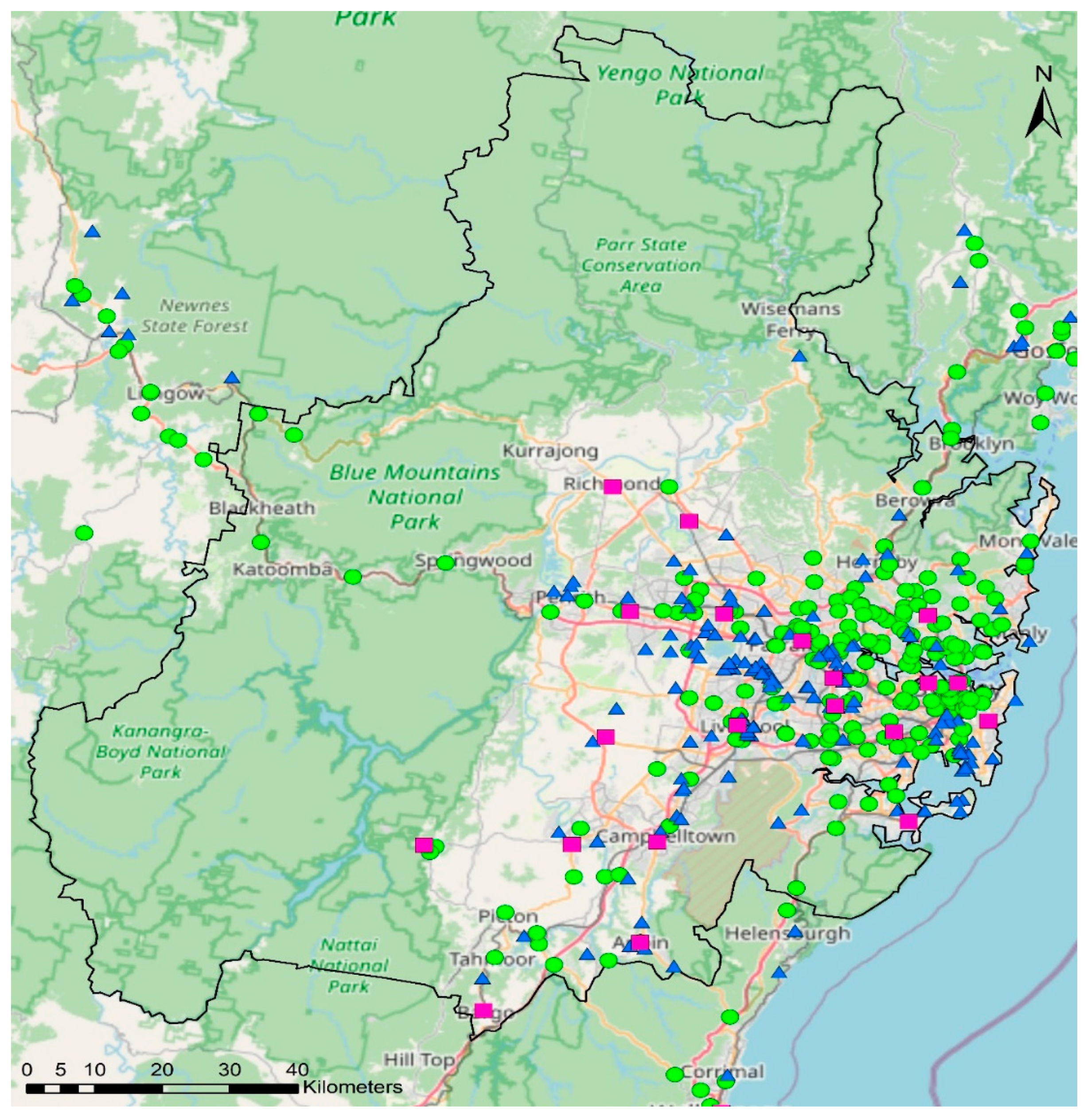
2.1. Study Area

This study focused on the Greater Sydney region as Sydney is the most populated city in Australia, with more than 5 M people [18]. Consequently, Sydney has a higher dwelling and population density, and a greater degree of urbanization compared to other Australian cities [19,20,21,22,23]. Sydney is situated along the mid-coast of New South Wales on a lowland plain between the Pacific Ocean to the east and elevated sandstone tablelands to the north, south, and west, creating the Sydney Basin [24]. Greater Sydney covers approximately 12,400 km2 and the profile of this basin has previously been associated with the transportation and accumulation of air pollutants produced within the area [25,26,27], thus making air quality a key concern for this international city. Additionally, Sydney is a complex mosaic of numerous anthropogenic activities, such as commercial, industrial, and agricultural, contributing to the accumulation of ambient air pollution, interspersed with natural areas, such as parklands and water bodies [22,23,28,29,30,31].

2.2. Data Preparation

2.2.1. Ambient Air Pollutant Concentrations

Ambient daily air pollutant concentrations for NO₂, SO₂, and PM₁₀ were incorporated in this study. The data was sourced from the NSW Government’s Department of Planning and Environment (DPE) monitoring network, which has air quality monitoring stations at 20 sites covering the entire Sydney basin region (Figure 1) [32,33,34]. Each monitoring station records air quality data hourly, in accordance with the National Environment and Protection Measures which is a national set of legally binding standards for air quality monitoring across Australia.

2.2.2. Industrial Pollutant Concentrations

Point source industrial pollutant concentrations for NO2, SO2, and PM10 were incorporated in this study. In Australia, there is a national scale database for reporting and monitoring industrial pollutant concentrations, named National Pollutant Inventory (NPI), which reports 93 substances [35]. It is managed by the Australian Government and monitors industrial facilities who have previously exceeded Australia’s legally binding air pollution thresholds [35]. Despite the wide range of NPI pollutant data and their public availability, the NPI data has been underutilised in research areas, particularly for analysing ambient air pollution. Thus, NPI pollutant data from 168 NPI monitored sites within and surrounding Sydney were used for each air pollutant and incorporated in this study (Figure 1). The NPI uses NOₓ as a surrogate for NO₂ emissions, as NOx is conventionally expressed as a NO₂ mass equivalent, and NO₂ is the most predominant form of atmospheric NOₓ [36].
Figure 1. The NSW DEP monitoring sites represented by pink squares [32,33,34]. The blue triangles represent the National Pollutant Inventory industrial locations [35]. The traffic data collection points are represented by the green circles [37].
Environments 10 00032 g001

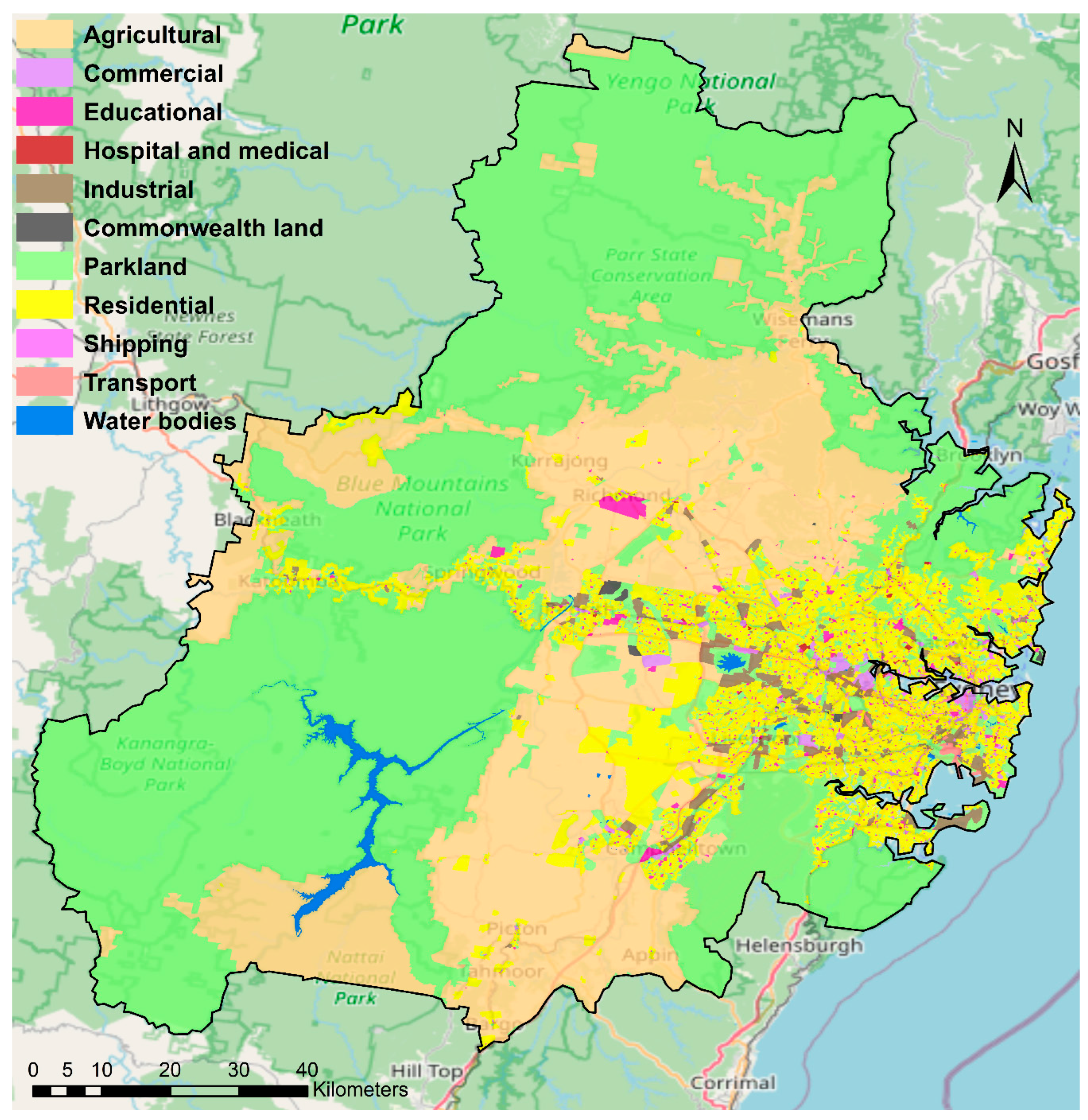
2.2.3. Land-Use Cover

Land use data consisted of planning and zoning data provided by the Australian Bureau of Statistics, which categorised land-use types into 11 different definitions during the 2006 Australian Census. Despite this data originating from the 2006 Australia Census, the data retained a high degree of accuracy and temporal relevance to the 2008 study period, as it was updated in August 2007 (Table 1, Figure 2) [38].

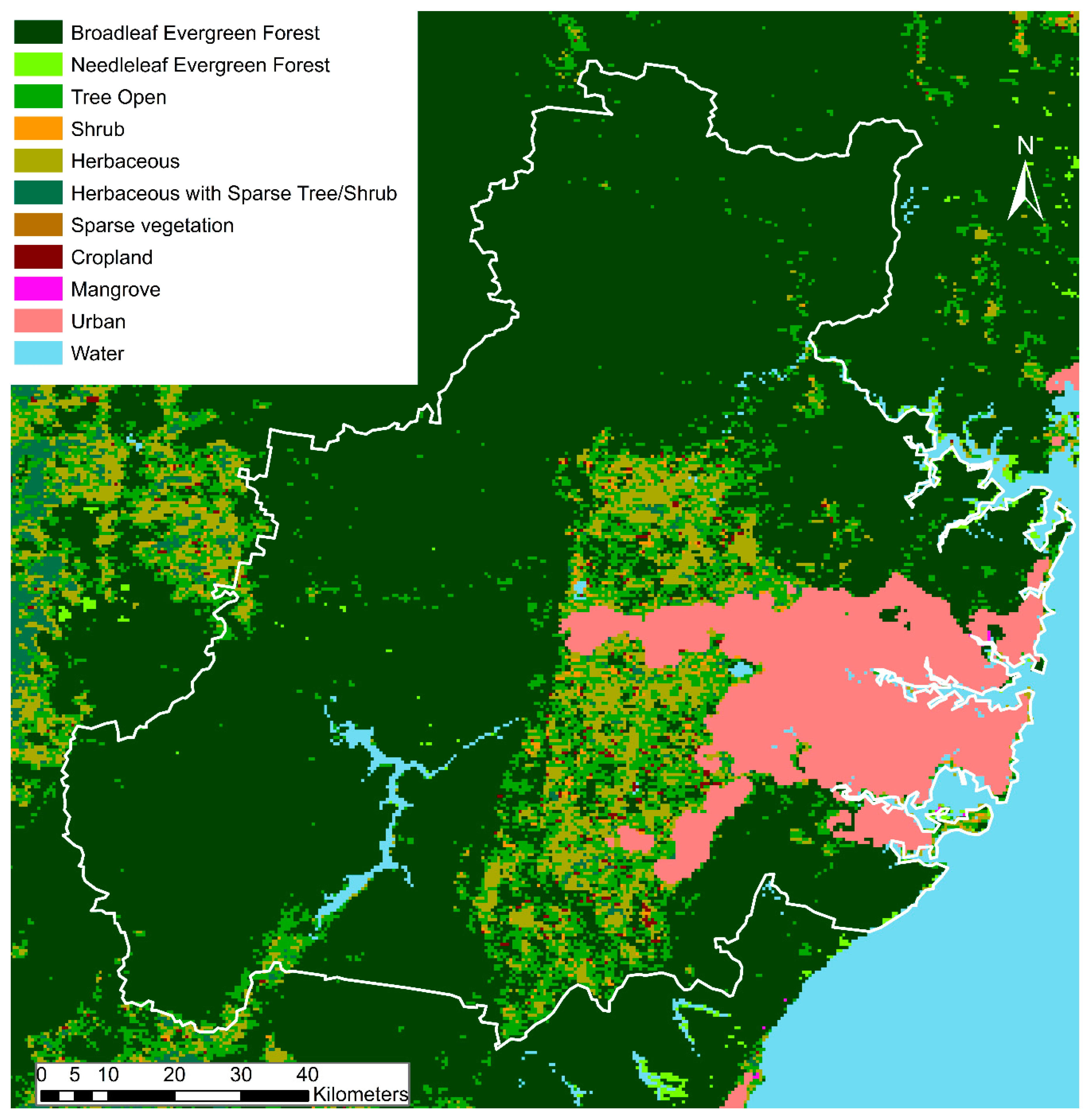
2.2.4. Urban Forestry Cover

Urban forestry cover data was obtained from the Global Mapping Project (GMP), which was developed through the incorporation of MODIS and Landsat data, Virtual Earth, existing regional and local maps, and existing land-cover products [39]. The spatially relevant data set included nine vegetation types and two urban land covers, water, and artificial surfaces (Figure 3, Table 2).

2.2.5. Daily Traffic Count

The daily traffic count data was used to correct for traffic density and subsequent traffic derived air pollution, with the data from 211 Roads and Maritime Services (RMS) traffic collection sites across Sydney annually averaged for daily traffic count and then spatially interpolated (Figure 1). The traffic data included count data for all vehicle types and directions of travel [37].

2.3. Overlay and Analysis

All data was transformed to the Geocentric Datum of Australia 1994 [40] and annually averaged within the same study period, 2008, thus randomising potentially confounding factors such as wildfires, hazard reduction burns, and seasonal and meteorological effects, such as wind, that have been identified in previously published air pollutant studies [8,25,41,42,43,44]. The sensitivity for this type of investigation is strongly dependent on the spatial resolution of the analyses in order to show clear spatial distributions and trends, identifying associations between air quality, vegetation, and other influential variables such as traffic, population density, or other anthropogenic activities [45,46,47]. Thus, a high pixel resolution of 30 m2 was used for this investigation.
The analytical method applied in this study was based on methods previously established by the European Study of Cohorts for Air Pollution Effects [42,43] with the incorporation of additional urban metrics and air pollutants. All data was transformed to the same spatial resolution and spatially joined. ArcGIS version 10.3.1 (ESRI Inc., Redlands, CA, USA) was used for all spatial processing, interpolation, transformations, joining, and map creation while statistical processing, analyses, and visualisations were performed in SPSS version 24 (Chicago, IBM SPSS, Inc., Chicago, IL, USA) and Microsoft Excel 2016 (Microsoft Corp., Redmond, WA, USA).
A general linear model and single factor analyses of covariance (ANCOVAs) were generated and compared for each of the three air pollutants amongst land-use and urban forestry types. NPI industrial concentrations and RMS traffic data were incorporated as covariables to correct for air pollutant source. Pairwise comparisons were made using Bonferroni’s post hoc tests [48] and estimated marginal means (EMMs) were derived from the ANCOVAs to control for the predicted high Type I error rate for the univariate statistical analyses [48,49,50]. Finally, all univariate contrasts were confirmed through the determination of whether the 95% confidence interval for an EMM overlapped with the EMM of another group.
The first exploratory model utilised the 11 different land-use types (Section 2.2.3) to identify spatial associations between land use and air pollutant concentrations. The second model utilised urban forestry data to identify associations between different vegetation types (Section 2.2.4) and air pollutant concentrations to facilitate a greater understanding about the potential for different vegetation types influencing pollutant concentrations.

3. Results

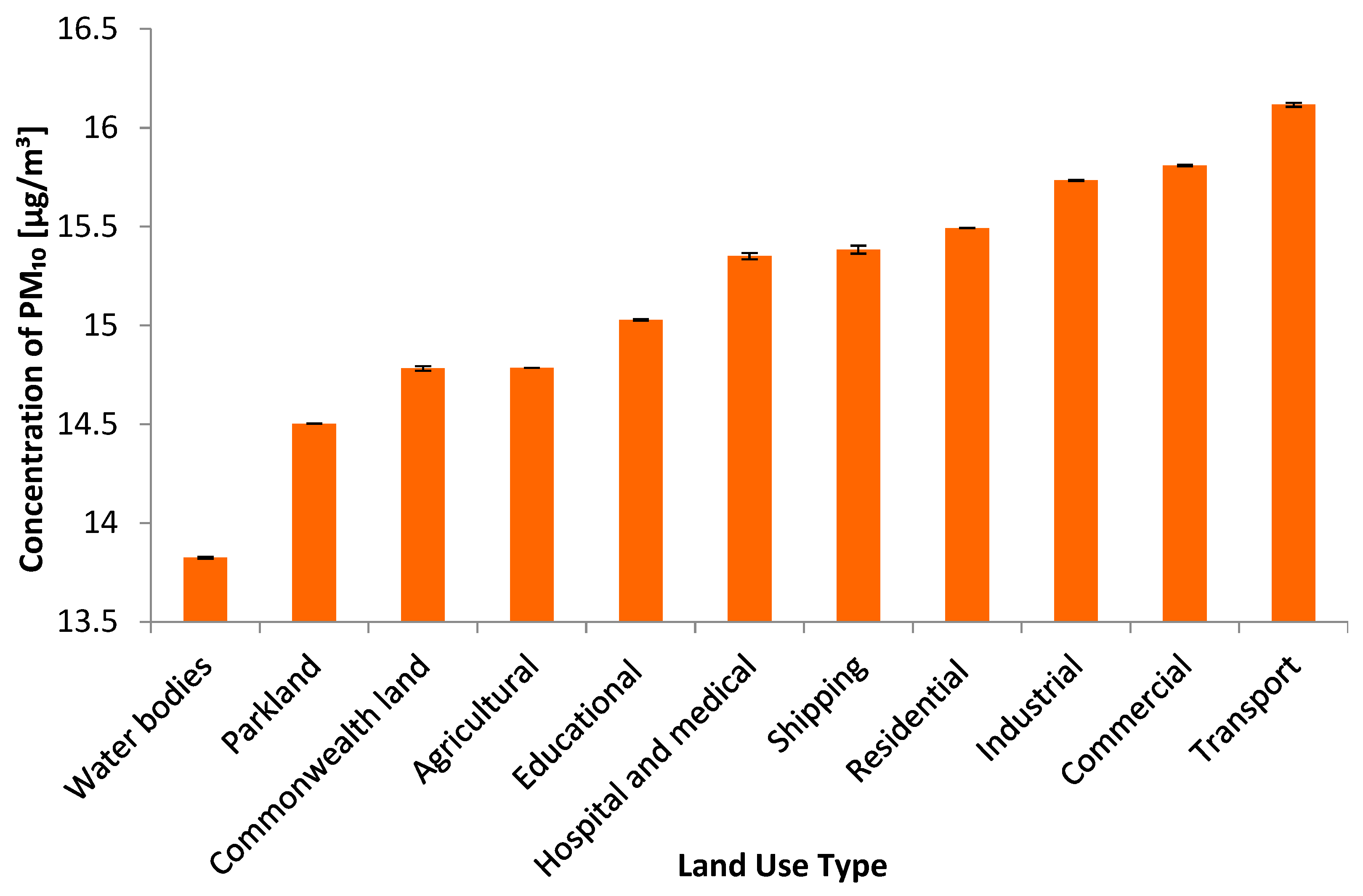
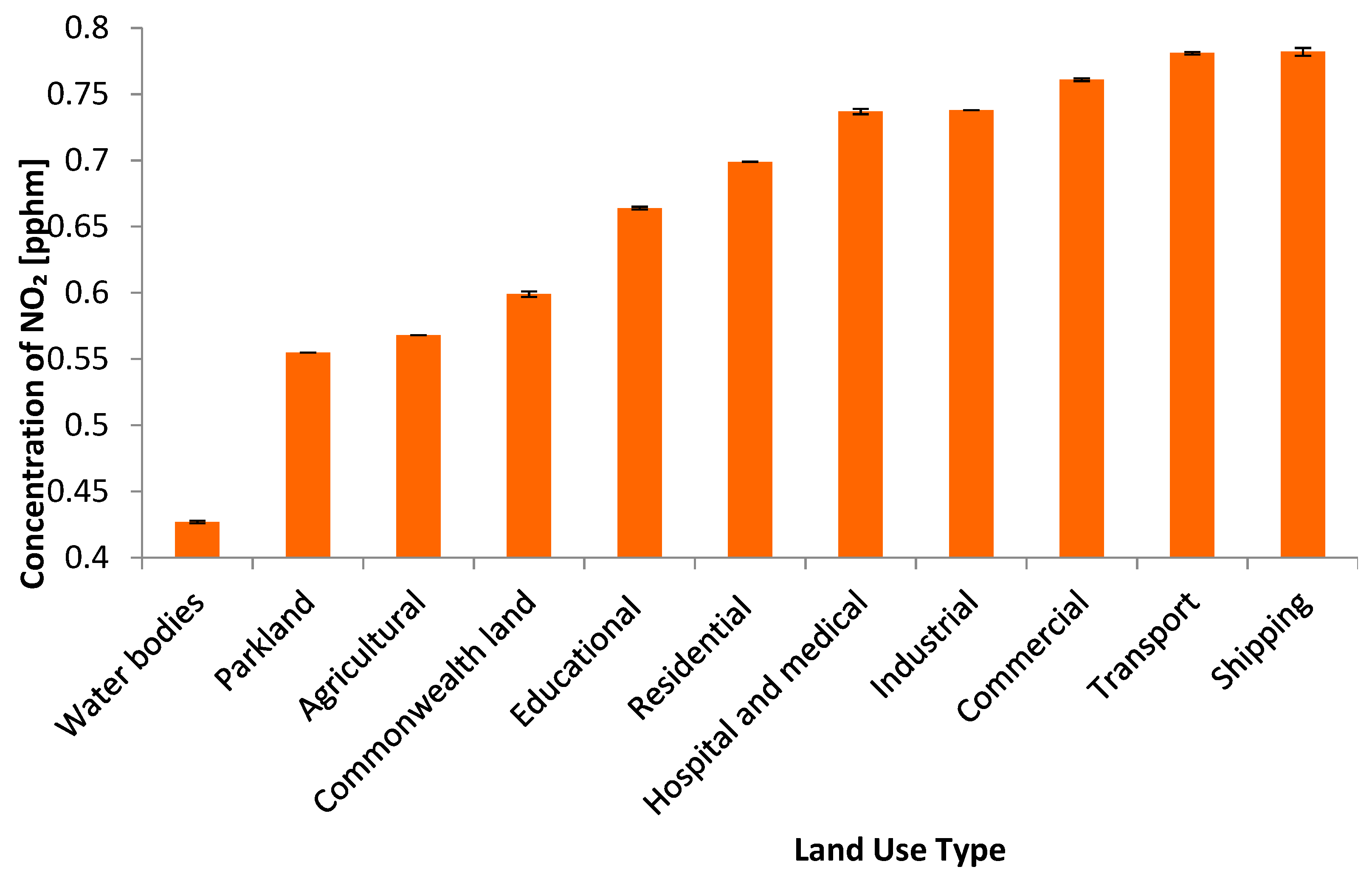
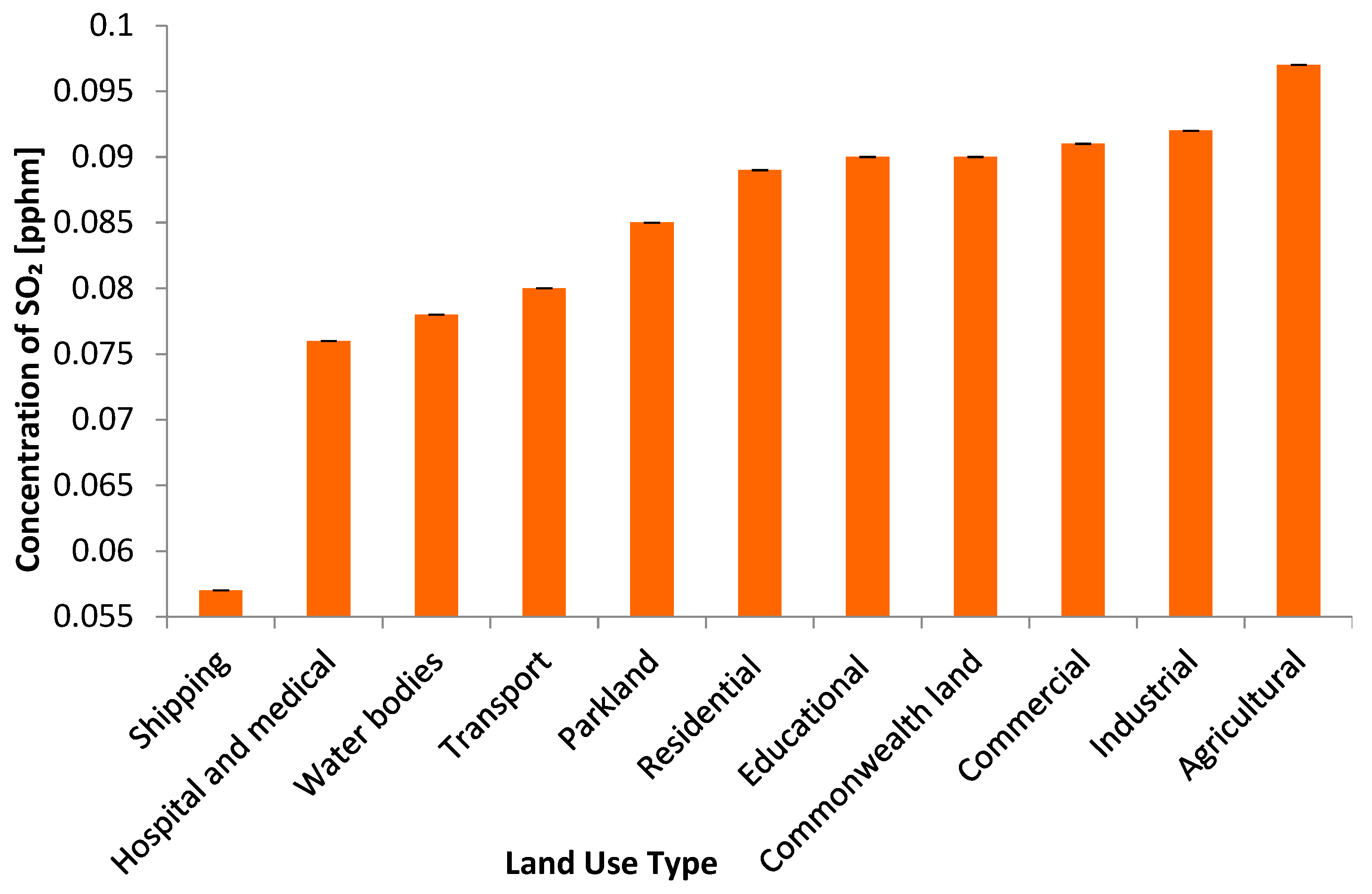
3.1. The Effects of Urban Land Use on Air Pollutant Concentrations

All three air pollutant concentrations were positively and significantly associated with the covariables, traffic density and NPI pollutants (Table 3; p < 0.05), with SO2 having the strongest association with the covariables, and PM₁₀ having the weakest linear spatial relationship with traffic, and NO2 weakly associated with the NPI industrial pollutants (Table 3).
ANCOVAs with Bonferroni’s post hoc tests were used to test for differences in air pollutant concentrations amongst the different land-use types (Figure 4, Figure 5 and Figure 6) after controlling for the effects of source, in the form of traffic and NPI industrial pollution. The residual variation in the data (estimated marginal means; EMMs) was used as a dependent data variable and analysed univariately to test the potential effect of land-cover type on ambient air pollutant concentrations (Figure 4, Figure 5 and Figure 6).
The general trend in the exploratory model indicated a significant association between vegetation and lower air pollutant concentrations, with parklands being associated with lower concentrations for all air pollutants except SO2 (Figure 4 and Figure 5). PM10 and NO2 shared similar concentration patterns, as their lowest concentrations occurred in areas categorised as water bodies and parklands (Figure 4 and Figure 5), while shipping land use was associated with the lowest SO2 levels (Figure 6).
Areas categorised as commercial, transport, and industrial land use demonstrated high concentrations for all pollutants. PM₁₀ had the highest concentrations in transport-related areas and NO₂ in shipping-related areas (Figure 4 and Figure 5). SO2 displayed a different pattern, with the highest concentrations being associated with agricultural land (Figure 6).

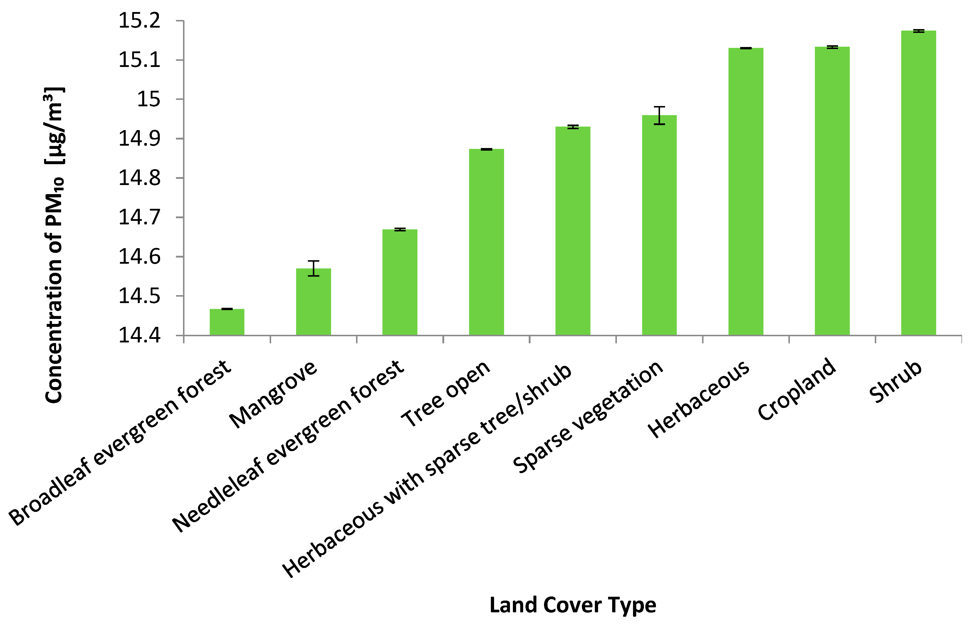
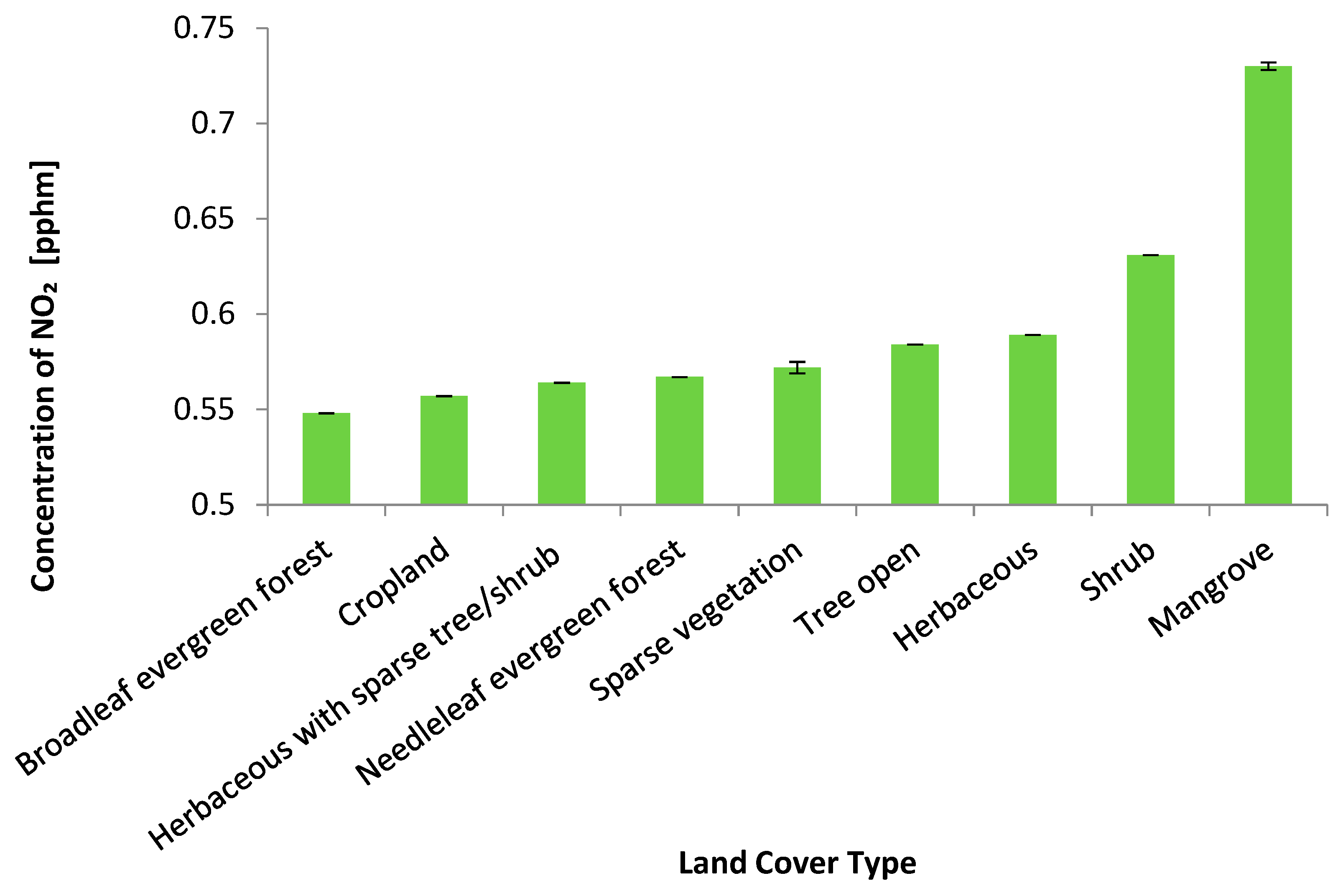
3.2. The Effects of Different Urban Forestry Types on Air Pollutant Concentrations

The associations between the air pollutants and covariables, traffic density and NPI pollutants, are shown in Table 4. All associations were statistically significant (p < 0.05), with each air pollutant following a similar trend to the previous exploratory model. Associations between air pollutant concentrations and proximity to source were indicated by the partial eta-squared values, with SO2 having the strongest association with both covariables and PM10 having the weakest linear spatial relationship with traffic, and NO2 weakly associated with the NPI industrial pollutants (Table 4).
ANCOVAs with Bonferroni’s post hoc tests were used to test for differences in air pollutant concentrations amongst areas with different vegetation types, and the subsequent EMMs were analysed univariately to test the potential associations between vegetation type on ambient air pollutant concentrations (Figure 7, Figure 8 and Figure 9).
SO2 and PM10 air pollutants demonstrated lower concentration EMMs for areas covered by broadleaf evergreen forest and mangroves, except for NO2 which only demonstrated low concentrations for broadleaf evergreen forests (Figure 7, Figure 8 and Figure 9). The higher concentrations for SO2 and PM10 were found in either shrubland or croplands, except for NO2 which exhibited its highest concentrations in mangrove areas (Figure 8) and SO2 with areas with sparse vegetation (Figure 9).

4. Discussion

4.1. General Overview

The current research has investigated the relationship between source-corrected air pollutant concentrations and urban areas, with particularly high levels detected in areas with anthropocentric-based land uses coupled with a lack of vegetation. The correction for anthropogenic sources ensured the spatial relationships between land-use or vegetation type and air pollutants were explicitly tested. Consequently, the associations between land uses such as transport, commercial, and industrial-related activities, and high level of ambient air pollution were confirmed. Contrastingly, the significant association detected between parklands and low pollutant concentration demonstrated the impact of vegetation and its ability to influence air pollutant concentrations in an urban environment.
Although urban forestry has generally been associated with improved air quality [8,51,52,53], few studies have investigated the potential of different vegetation types on an entire city scale with air pollution mitigation. The current research found different types of vegetation influenced air pollutants differently with broadleaf evergreen forests generally tending to be associated with lower air pollutant concentrations. While this study did not manipulatively appraise the causality of the relationship between urban forestry and air pollution, the associated findings align with existing findings, providing further support that such a causal pattern may exist.

4.2. The Inclusion of NPI Industrial Concentrations and Traffic Data

Traffic density and industrial pollution were added as covariables to correct for pollutant source and ensure the main effects of land-use and vegetation type were investigated in this study. The influence of these were elucidated as all pollutants were positively and significantly associated with the covariables across both exploratory models, with SO2 having the strongest association with both and PM10 having the weakest with traffic and NO2 with the NPI industrial pollutants. Interestingly, the weak association between PM and traffic density was in contrast to the other published literature as increased incomplete combustion tends to occur in traffic dense areas or during periods of heavy traffic congestion [54,55,56]. This difference in findings may be driven by traffic conditions being strongly related to the diurnal peak hour patterns, in which case the use of annual averages in these exploratory models may have had insufficient temporal resolution to detect these associations [57,58].
The significant pollutant associations with the NPI industrial concentrations were novel in their own right, as NPI industrial data had not been frequently incorporated into exploratory models such as those presented here, and they confirmed the impact of industrial pollution point sources on ambient air quality. The significantly strong association with SO2 is possibly driven by the types of industries represented in this dataset, which includes a wide range of industrial processing and manufacturing facilities [35]. Consequently, these findings also highlighted the potential for incorporation of these kind of datasets into future research.

4.3. The Associations between Different Urban Land Uses and Air Pollutant Concentrations

Areas categorised as commercial, transport, and industrial land use demonstrated high concentrations for all pollutants, while parklands were associated with lower concentrations of PM10 and NO2 and shipping was associated with the lowest SO2 concentrations. Parklands were associated with lower PM10 concentrations in the current study, an effect that has previously been observed in other air pollution models, with urban forestry negatively contributing to PM in models from Finland, Denmark, United Kingdom, Germany, Austria, Hungary, Switzerland, Italy, and Spain [59]. Ambient PM can be deposited on plants, this occurs when suspended particulate matter is deposited onto the surface of a plant through impaction, interception, settling, or diffusion [60]. A plant’s morphological characteristics could increase its particulate capture, with hairy or rough bark or leaves, complex structures, larger surface areas, and waxy epicuticular layers associated with increased PM deposition [61,62]. Similarly, the low NO2 concentrations across parklands was also due to the mitigating effects of vegetation. A previous study from Sydney found that air pollution was negatively correlated with tree canopy cover and found a statistically significant spatial relationship between urban forestry and air pollution [8]. Jayasooriya et al. [63] modelled air pollution removal through urban forestry in an industrial precinct in Victoria, Australia, and found that urban forestry had the potential to remove NO2, SO2, and PM10. The value of urban forestry in Sydney was also outlined by Lin et al. [22], who found it had the potential to provide a wide range of ecosystem benefits, including air pollutant removal. Brack [64] assessed the ecosystem services of trees in Canberra, Australia, and found that the contribution of urban trees to the reduction of energy consumption, amelioration of air pollution, and the improvement to local hydrology had an estimated annual value of USD 20–67 million [64].
These trends are not exclusive to Australia, with cities globally experiencing similar outcomes when urban forestry is increased, despite the differences in climate, location, and anthropogenic influences [21,51,62,65]. A study from Taipei, Taiwan, found that both natural and seminatural urban green spaces had negative relationships with NOₓ and NO2 [66]. This relationship was confirmed by Klingberg et al. [52], who found vegetated sites across Gothenburg, Sweden, had lower NO2 concentrations than nonvegetated sites, while Cohen et al. [67] found urban parks across Israel were associated with lower concentrations of NOₓ and PM10 when compared with urban street canyons.
A spatially dependent mechanism for lower NO2 concentrations due to dilution effects from the presence of parklands and urban forests is possible [44,51,52,68]. Dilution occurs through an increase in the distance between the source of pollution and the point of sampling. Urban parklands and forestry are beneficial for anthropogenic pollutant dilution as they increase the distance from pollutant source without increasing anthropogenic pollutant concentrations [44,51,52]. Vegetated areas also provide a cleaner air source during photosynthetically active periods due to oxygen emission, thus further reducing the concentration of pollutants through atmospheric mixing [51,52].
The association between water bodies and lower PM10 may have been due to multiple factors. The majority of the water bodies are proximal to parklands (Figure 2), which may have led to a spatial confound in the detected pattern. Additionally, simulations of cities with no urban water bodies have demonstrated increased wind speeds, which could allow particulate matter to remain suspended in the air column [69], while urban areas with natural or artificial water bodies may experience decreased wind speeds [69], facilitating particle deposition [51,70,71].
Anthropogenic SO2 emissions are largely related to the combustion of sulphur-rich coal and other fossil fuels, which are used in a wide range of sectors, including residential heating and cooking, industrial processing and manufacturing, electricity generation, and shipping [41,72,73,74]. However, in the current study, the highest SO2 concentrations were associated with agriculture, followed by industrial and commercial land uses. The association between low SO2 concentrations and shipping, seen in this current study, could have been driven by the growing use of low-emission fuels necessitated by global demand for the reduction in shipping-related pollutants [75,76,77]. Furthermore, efficient dispersion of SO2 along Sydney’s coast, where the majority of shipping facilities are located, would have also influenced its concentration [78,79,80]. Additionally, shipping facilities are not a main source of pollution, but the vessels themselves [75,79]. The relatively low output of shipping exhaust and the effect of the proximal water bodies and wind effects are likely reasons for the observed low pollutant levels in these areas.
High NO2 concentrations in the current model were associated with transportation, commercial, and shipping land uses. This relationship is driven by petrol and diesel engines, which account for over 80% of NOx emissions, with NO2 being the most prevalent form of atmospheric NOₓ [36,81]. Additionally, the combustion of fossil fuels and industrial processes associated with diverse commercial activities and production are strongly correlated with NO2 [21,52,82]. The current findings support previous studies conducted across Australia [19,21,29,31,83], Western Turkey [84], Thailand [85], and Canada [86].
The high concentrations of SO2 in agricultural areas was unexpected, although the current observations align with an emerging understanding of the relationship between SO2 and agricultural activities [87,88,89,90]. SO2 can have impacts on human and animal health along with the surrounding environment [88,89,90]. Human and animal health impacts are especially prevalent in livestock houses that collect animal waste in manure pits underneath slatted floors above which the animals reside [88]. While the exact mechanisms and behaviour of this relationship requires further research, SO2 is believed to be released from primarily organic wastes, animal manure, wastewater, and the disruption of acid sulphate soils during agricultural activities [87,88,89,90]. Additionally, the release of SO2 is the main precursor to acid rain which can contribute to the acidification of soils, lakes, and streams [88,89,90].

4.4. The Association between Different Urban Forestry Types and Air Pollutant Concentrations

Air pollutants SO2 and PM10 demonstrated lower concentrations in areas covered by broadleaf evergreen forest and mangroves while NO2 only demonstrated low concentrations for broadleaf evergreen forests. The higher concentrations for SO2 and PM10 were found in croplands while NO2 exhibited high concentrations in mangrove areas. In the current study, PM10 concentrations were high in areas of shrub and croplands. These vegetation types were clustered at the western side of the study area, which is considered semiarid and drought-prone, which may have driven this association [91]. Sydney experienced a prolonged and widespread drought from 2000 to 2009 [27,91], which would have contributed to increased levels of atmospheric PM₁₀ from wind-blown dust [27].
Broadleaf evergreen forests and needleleaf evergreen forests were associated with lower ambient PM10 concentrations, which aligns with the findings from previous research [14,60,68,92,93,94]. The leaf and plant characteristics present across both broadleaf and needleleaf evergreen species such as hairy plant surfaces, waxy epicuticular layers, complex plant structures, larger surfaces areas, and increased and prolonged vegetation/canopy density throughout the year are all known to enhance PM accumulation [14,53,60,68,93,95].
Mangroves also had a noticeable association with low air pollutant concentrations for PM10 in the current study. Such effects have not been detected previously. Mangroves are coastal forests found in sheltered estuaries and along river banks and lagoons [96,97]. There are several potential explanations for the observed air pollution remediation effect. Similar to the broadleaf and needleleaf evergreen forests, mangrove canopy cover is usually dense, with more than 70% cover, the leaves are waxy, and the plants possess complex and woody structures, thus potentially assisting with deposition of particulates [53,82,93,94,96,97]. Additionally, the majority of Sydney’s mangroves are surrounded by broadleaf evergreen forests (Figure 3). These proximal vegetation types may have led to general area effects where air pollutants were removed by a range of independent mechanisms.
The association between low concentrations of NO2 and broadleaf evergreen forests in this study supports the findings of Leung et al. [53] and Currie and Bass [98], who found that leaf longevity and continuous photosynthetic performance throughout the seasons enables greater gaseous pollutant sequestration in this vegetation type. Gaseous pollutant uptake is dependent on stomatal conductance and photosynthetic capacity. Stomatal conductance is in turn dependent on leaf properties such as leaf area and orientation, while photosynthetic capacity is dependent on the leaf type and formation [99,100]. Both of these favourable traits are prevalent in broadleaf evergreen forests [99,100,101].
The association between croplands and high SO2 concentrations aligned with the previously discussed association between SO2 and agriculture and with previous research [87,88,89,90,102], while lower SO2 concentrations were detected in areas with mangroves and broadleaf evergreen forests. The mechanisms behind these effects are likely similar to those proposed for NO2 previously. Interestingly, the favourable traits for gaseous pollutant mitigation in broadleaf evergreen forests are also present in mangroves, which could explain the association with low SO2 concentrations in the current study. Most mangrove trees are evergreen with sclerophyllous leaves that have an average leaf life span of 16 months, similar to other terrestrial evergreen species [103,104]. Additionally, the proximity to broadleaf evergreen forest may have combined to lead to general area effects.
Conversely, mangroves had a noticeable association with high concentrations of NO2 in the current study. Mangroves in their natural state act as a sink for nitrogen [105,106]. However, modification of their biochemical processes due to anthropogenic nutrification and denitrification, along with increased nitrogen loading, may alter these processes resulting in mangroves acting as sources of atmospheric nitrogen [105,106,107]. Furthermore, all of the mangrove sites within the current study could have been influenced by anthropogenic effects due to proximity to urban areas, potentially influencing the detected association with NO2.

5. Conclusions

The present research provides an insight into the associations between vegetation and air pollution in order to quantify and evaluate the spatial variation of air pollutant concentrations associated with different forms of urban forestry. The incorporation of anthropogenic pollutant sources ensured that the hypothesis that urban forestry was associated with air pollution removal was explicitly tested. Associations between different vegetation types and air pollutant concentrations were established, with broadleaf evergreen forests consistently associated with lower pollutant concentrations. Areas classified as parklands and water bodies displayed consistently lower air pollution concentrations, confirming the negative association between urban forestry and ambient air pollution concentrations on a city-wide scale. The statistically significant association between urban forestry and low air pollutant concentrations promotes the value of urban forestry, while the vegetation insights may provide a foundation for future research into targeted vegetation applications to provide the greatest air quality benefits.

Author Contributions

Conceptualization, A.N.J.D., P.J.I. and F.R.T.; methodology, A.N.J.D., P.J.I. and F.R.T.; software, A.N.J.D.; validation, P.J.I. and F.R.T.; formal analysis, A.N.J.D.; investigation, A.N.J.D.; writing—original draft preparation, A.N.J.D.; writing—review and editing, P.J.I. and F.R.T.; supervision, P.J.I. and F.R.T.; project administration, A.N.J.D. All authors have read and agreed to the published version of the manuscript.

Funding

This research was funded by an Australian Government Research Training Program Scholarship for A.N.J.D.

Data Availability Statement

The data used for this study is held by the authors. Please contact the corresponding author for details.

Acknowledgments

The authors would like to thank Malcolm Frederick Douglas and Gail Annette Douglas.

Conflicts of Interest

The authors declare no conflict of interest.

References

  1. McDonnell, M.J.; MacGregor-Fors, I. The ecological future of cities. Science 2016, 352, 936–938. [Google Scholar] [CrossRef]
  2. World Health Organisation. Ambient (Outdoor) Air Pollution: World Health Organisation. 2021. Available online: https://www.who.int/news-room/fact-sheets/detail/ambient-(outdoor)-air-quality-and-health (accessed on 16 December 2022).
  3. WHO Regional Office for Europe; OECD. Economic Cost of the Health Impact of Air Pollution in Europe: Clean Air, Health and Wealth; World Health Organization: Geneva, Switzerland, 2015; p. 62. [Google Scholar]
  4. Hewitt, C.N.; Ashworth, K.; MacKenzie, A.R. Using green infrastructure to improve urban air quality (GI4AQ). Ambio 2020, 49, 62–73. [Google Scholar] [CrossRef] [Green Version]
  5. Isaifan, R. The dramatic impact of Coronavirus outbreak on air quality: Has it saved as much as it has killed so far? Global J. Environ. Sci. Manag. 2020, 6, 275–288. [Google Scholar]
  6. Zeng, Y.; Cao, Y.; Qiao, X.; Seyler, B.C.; Tang, Y. Air pollution reduction in China: Recent success but great challenge for the future. Sci. Total Environ. 2019, 663, 329–337. [Google Scholar] [CrossRef] [PubMed]
  7. Kumar, P.; Druckman, A.; Gallagher, J.; Gatersleben, B.; Allison, S.; Eisenman, T.S.; Hoang, U.; Hama, S.; Tiwari, A.; Sharma, A.; et al. The nexus between air pollution, green infrastructure and human health. Environ. Int. 2019, 133, 105181. [Google Scholar] [CrossRef]
  8. Douglas, A.N.J.; Irga, P.J.; Torpy, F.R. Determining broad scale associations between air pollutants and urban forestry: A novel multifaceted methodological approach. Environ. Pollut. 2019, 247, 474–481. [Google Scholar] [CrossRef]
  9. Hu, Y.; Zhao, P.; Niu, J.; Sun, Z.; Zhu, L.; Ni, G. Canopy stomatal uptake of NOX, SO2 and O3 by mature urban plantations based on sap flow measurement. Atmos. Environ. 2016, 125, 165–177. [Google Scholar] [CrossRef]
  10. Chaparro-Suarez, I.G.; Meixner, F.X.; Kesselmeier, J. Nitrogen dioxide (NO2) uptake by vegetation controlled by atmospheric concentrations and plant stomatal aperture. Atmos. Environ. 2011, 45, 5742–5750. [Google Scholar] [CrossRef]
  11. Gong, C.; Xian, C.; Su, Y.; Ouyang, Z. Estimating the nitrogen source apportionment of Sophora japonica in roadside green spaces using stable isotope. Sci. Total Environ. 2019, 689, 1348–1357. [Google Scholar] [CrossRef]
  12. Liang, D.; Ma, C.; Wang, Y.-Q.; Wang, Y.-J.; Zhao, C.-X. Quantifying PM 2.5 capture capability of greening trees based on leaf factors analyzing. Environ. Sci. Pollut. Res. 2016, 23, 21176–21186. [Google Scholar] [CrossRef] [Green Version]
  13. Nguyen, T.; Yu, X.; Zhang, Z.; Liu, M.; Liu, X. Relationship between types of urban forest and PM2.5 capture at three growth stages of leaves. J. Environ. Sci. 2015, 27, 33–41. [Google Scholar] [CrossRef] [PubMed]
  14. Leonard, R.J.; McArthur, C.; Hochuli, D.F. Particulate matter deposition on roadside plants and the importance of leaf trait combinations. Urban For. Urban Green. 2016, 20, 249–253. [Google Scholar] [CrossRef]
  15. King, K.L.; Johnson, S.; Kheirbek, I.; Lu, J.W.T.; Matte, T. Differences in magnitude and spatial distribution of urban forest pollution deposition rates, air pollution emissions, and ambient neighborhood air quality in New York City. Landsc. Urban Plan. 2014, 128, 14–22. [Google Scholar] [CrossRef]
  16. Eisenman, T.S.; Churkina, G.; Jariwala, S.P.; Kumar, P.; Lovasi, G.S.; Pataki, D.E. Urban trees, air quality, and asthma: An interdisciplinary review. Landsc. Urban Plan. 2019, 187, 47–59. [Google Scholar] [CrossRef]
  17. Rao, M.; George, L.A.; Rosenstiel, T.N.; Shandas, V.; Dinno, A. Assessing the relationship among urban trees, nitrogen dioxide, and respiratory health. Environ. Pollut. 2014, 194, 96–104. [Google Scholar] [CrossRef]
  18. Australian Bureau of Statistics. 3218.0–Regional Population Growth, Australia, 2016–2017 Australia: Commonwealth of Australia. 2018. Available online: http://www.abs.gov.au/ausstats/abs@.nsf/Latestproducts/3218.0Main%20Features12016-17?opendocument&tabname=Summary&prodno=3218.0&issue=2016-17&num=&view= (accessed on 10 April 2018).
  19. Dirgawati, M.; Barnes, R.; Wheeler, A.J.; Arnold, A.-L.; McCaul, K.A.; Stuart, A.L.; Blake, D.; Hinwood, A.; Yeap, B.B.; Heyworth, J.S. Development of Land Use Regression models for predicting exposure to NO2 and NOx in Metropolitan Perth, Western Australia. Environ. Model. Softw. 2015, 74, 258–267. [Google Scholar] [CrossRef]
  20. Knibbs, L.D.; Barnett, A.G. Assessing environmental inequalities in ambient air pollution across urban Australia. Spat. Spatio-Temporal Epidemiol. 2015, 13, 1–6. [Google Scholar] [CrossRef]
  21. Knibbs, L.D.; Hewson, M.G.; Bechle, M.J.; Marshall, J.D.; Barnett, A.G. A national satellite-based land-use regression model for air pollution exposure assessment in Australia. Environ. Res. 2014, 135, 204–211. [Google Scholar] [CrossRef] [Green Version]
  22. Lin, B.; Meyers, J.; Barnett, G. Understanding the potential loss and inequities of green space distribution with urban densification. Urban For. Urban Green. 2015, 14, 952–958. [Google Scholar] [CrossRef]
  23. Rose, N.; Cowie, C.; Gillett, R.; Marks, G.B. Validation of a Spatiotemporal Land Use Regression Model Incorporating Fixed Site Monitors. Environ. Sci. Technol. 2011, 45, 294–299. [Google Scholar] [CrossRef]
  24. Gero, A.F.; Pitman, A.J.; Narisma, G.T.; Jacobson, C.; Pielke, R.A. The impact of land cover change on storms in the Sydney Basin, Australia. Glob. Planet. Chang. 2006, 54, 57–78. [Google Scholar] [CrossRef]
  25. Legislative Council. Health Impacts of Air Pollution in the Sydney Basin; New South Wales Parliament: Sydney, Australia, 2006. [Google Scholar]
  26. Duc, H.; Azzi, M.; Wahid, H.; Ha, Q.P. Background ozone level in the Sydney basin: Assessment and trend analysis. Int. J. Climatol. 2013, 33, 2298–2308. [Google Scholar] [CrossRef]
  27. Cohen, D.D.; Stelcer, E.; Garton, D.; Crawford, J. Fine particle characterisation, source apportionment and long-range dust transport into the Sydney Basin: A long term study between 1998 and 2009. Atmos. Pollut. Res. 2011, 2, 182–189. [Google Scholar] [CrossRef] [Green Version]
  28. Cowie, C.T.; Ding, D.; Rolfe, M.I.; Mayne, D.J.; Jalaludin, B.; Bauman, A. Neighbourhood walkability, road density and socio-economic status in Sydney, Australia. Environ. Health 2016, 15, 58. [Google Scholar] [CrossRef] [Green Version]
  29. Knibbs, L.D.; Coorey, C.P.; Bechle, M.J.; Cowie, C.T.; Dirgawati, M.; Heyworth, J.S. Independent Validation of National Satellite-Based Land-Use Regression Models for Nitrogen Dioxide Using Passive Samplers. Environ. Sci. Technol. 2016, 50, 12331–12338. [Google Scholar] [CrossRef] [Green Version]
  30. Marquez, L.; Salim, V. Assessing impacts of urban freight measures on air toxic emissions in Inner Sydney. Environ. Model. Softw. 2007, 22, 515–525. [Google Scholar] [CrossRef]
  31. Rahman, M.M.; Yeganeh, B.; Clifford, S.; Knibbs, L.D.; Morawska, L. Development of a land use regression model for daily NO2 and NOx concentrations in the Brisbane metropolitan area, Australia. Environ. Model. Softw. 2017, 95, 168–179. [Google Scholar] [CrossRef] [Green Version]
  32. Department of Planning, Industry and Environment. Air Quality Data Services New South Wales: New South Wales Government. 2022. Available online: http://www.environment.nsw.gov.au/AQMS/search.htm (accessed on 15 July 2022).
  33. Department of Planning, Industry and Environment. Air Quality Monitoring Network New South Wales: New South Wales Government. 2022. Available online: https://www.environment.nsw.gov.au/topics/air/monitoring-air-quality (accessed on 15 July 2022).
  34. Department of Planning, Industry and Environment. Air New South Wales: New South Wales Government. 2022. Available online: http://www.environment.nsw.gov.au/topics/air (accessed on 15 July 2022).
  35. Department of the Environment. National Pollutant Inventory Guide Canberra: Commonwealth of Australia. 2015. Available online: http://www.npi.gov.au/resource/national-pollutant-inventory-guide (accessed on 17 April 2017).
  36. Boulter, P.G.; Borken-Kleefeld, J.; Ntziachristos, L. The Evolution and Control of NOx Emissions from Road Transport in Europe. In Urban Air Quality in Europe; Viana, M., Ed.; Springer: Berlin/Heidelberg, Germany, 2013; pp. 31–53. [Google Scholar]
  37. Roads and Maritime Services. Traffic Volume Viewer New South Wales: Roads and Maritime Services. 2008. Available online: http://www.rms.nsw.gov.au/about/corporate-publications/statistics/traffic-volumes/aadt-map/index.html#/?z=6 (accessed on 20 February 2017).
  38. Australian Bureau of Statistics. 1209.0.55.002–Mesh Blocks Digital Boundaries, Australia, 2006 Australia: Commonwealth of Australia. 2009. Available online: http://www.abs.gov.au/AUSSTATS/abs@.nsf/Lookup/1209.0.55.002Main+Features12006?OpenDocument (accessed on 17 April 2017).
  39. Tateishi, R.; Hoan, N.T.; Kobayashi, T.; Alsaaideh, B.; Tana, G.; Phong, D.X. Production of Global Land Cover Data–GLCNMO2008. J. Geogr. Geol. 2014, 6, 99. [Google Scholar] [CrossRef] [Green Version]
  40. Geoscience Australia. Geocentric Datum of Australia (GDA) Canberra: Commonwealth of Australia. 2017. Available online: http://www.ga.gov.au/scientific-topics/positioning-navigation/geodesy/geodetic-datums/gda (accessed on 16 February 2017).
  41. Broome, R.A.; Fann, N.; Cristina, T.J.N.; Fulcher, C.; Duc, H.; Morgan, G.G. The health benefits of reducing air pollution in Sydney, Australia. Environ. Res. 2015, 143, 19–25. [Google Scholar] [CrossRef]
  42. European Study of Cohorts for Air Pollution Effects. Study Manual; Institute for Risk Assessment Sciences; Utrecht University: Utrecht, The Netherlands, 2008. [Google Scholar]
  43. European Study of Cohorts for Air Pollution Effects. Exposure Assessment Manual; Institute for Risk Assessment Sciences; Utrecht University: Utrecht, The Netherlands, 2010. [Google Scholar]
  44. Tiwari, A.; Kumar, P. Integrated dispersion-deposition modelling for air pollutant reduction via green infrastructure at an urban scale. Sci. Total Environ. 2020, 723, 138078. [Google Scholar] [CrossRef]
  45. Al Koas, K.A.A.A. GIS-Based Mapping and Statistical Analysis of Air Pollution and Mortality in Brisbane; Queensland University of Technology: Brisbane, Australia, 2010. [Google Scholar]
  46. Narashid, R.H.; Mohd, W.M.N.W. (Eds.) Air Quality Monitoring Using Remote Sensing and GIS Technologies. In Proceedings of the 2010 International Conference on Science and Social Research (CSSR 2010), Kuala Lumpur, Malaysia, 5–7 December 2010. [Google Scholar]
  47. Liu, T.; Yang, X. Monitoring land changes in an urban area using satellite imagery, GIS and landscape metrics. Appl. Geogr. 2015, 56, 42–54. [Google Scholar] [CrossRef]
  48. Field, A. Discovering Statistics Using SPSS; Sage Publications: New York, NY, USA, 2009. [Google Scholar]
  49. Becker, L.A. General Linear Model (GLM): 2-Way, Between-Subjects Designs Colorado: University of Colorado Colorado Springs. 1999. Available online: https://www.uccs.edu/lbecker/glm_2way.html (accessed on 27 July 2022).
  50. Garbin, C. 2xk 2-Factor Between Groups ANOVA with EMMEANS Follow-ups Lincoln, Nebraska: Univerisyt of Nebraska-Lincoln. 2015. Available online: http://psych.unl.edu/psycrs/942/q2/2xk_factorial_142.pdf (accessed on 30 July 2022).
  51. Janhäll, S. Review on urban vegetation and particle air pollution–Deposition and dispersion. Atmos. Environ. 2015, 105, 130–137. [Google Scholar] [CrossRef]
  52. Klingberg, J.; Broberg, M.; Strandberg, B.; Thorsson, P.; Pleijel, H. Influence of urban vegetation on air pollution and noise exposure–A case study in Gothenburg, Sweden. Sci. Total Environ. 2017, 599–600, 1728–1739. [Google Scholar] [CrossRef]
  53. Leung, D.Y.C.; Tsui, J.K.Y.; Chen, F.; Yip, W.-K.; Vrijmoed, L.L.P.; Liu, C.-H. Effects of Urban Vegetation on Urban Air Quality. Landsc. Res. 2011, 36, 173–188. [Google Scholar] [CrossRef]
  54. Chan, L.Y.; Lau, W.L.; Lee, S.C.; Chan, C.Y. Commuter exposure to particulate matter in public transportation modes in Hong Kong. Atmos. Environ. 2002, 36, 3363–3373. [Google Scholar] [CrossRef]
  55. Kim, K.-H.; Sul, K.-H.; Szulejko, J.E.; Chambers, S.D.; Feng, X.; Lee, M.-H. Progress in the reduction of carbon monoxide levels in major urban areas in Korea. Environ. Pollut. 2015, 207, 420–428. [Google Scholar] [CrossRef]
  56. Ward, H.; Kotthaus, S.; Grimmond, C.; Bjorkegren, A.; Wilkinson, M.; Morrison, W.; Evans, J.; Morison, J.; Iamarino, M. Effects of urban density on carbon dioxide exchanges: Observations of dense urban, suburban and woodland areas of southern England. Environ. Pollut. 2015, 198, 186–200. [Google Scholar] [CrossRef] [Green Version]
  57. Mazaheri, M.; Reche, C.; Rivas, I.; Crilley, L.R.; Álvarez-Pedrerol, M.; Viana, M.; Tobias, A.; Alastuey, A.; Sunyer, J.; Querol, X.; et al. Variability in exposure to ambient ultrafine particles in urban schools: Comparative assessment between Australia and Spain. Environ. Int. 2016, 88, 142–149. [Google Scholar] [CrossRef] [Green Version]
  58. Morawska, L.; Jayaratne, E.R.; Mengersen, K.; Jamriska, M.; Thomas, S. Differences in airborne particle and gaseous concentrations in urban air between weekdays and weekends. Atmos. Environ. 2002, 36, 4375–4383. [Google Scholar] [CrossRef] [Green Version]
  59. Eeftens, M.; Beelen, R.; de Hoogh, K.; Bellander, T.; Cesaroni, G.; Cirach, M. Development of Land Use Regression Models for PM2.5, PM2.5 Absorbance, PM10 and PMcoarse in 20 European Study Areas; Results of the ESCAPE Project. Environ. Sci. Technol. 2012, 46, 11195–11205. [Google Scholar] [CrossRef]
  60. Cai, M.; Xin, Z.; Yu, X. Spatio-temporal variations in PM leaf deposition: A meta-analysis. Environ. Pollut. 2017, 231 Pt 1, 207–218. [Google Scholar] [CrossRef] [PubMed]
  61. Weyens, N.; Thijs, S.; Popek, R.; Witters, N.; Przybysz, A.; Espenshade, J.; Gawrońska, H.; Vangronsveld, J.; Gawronski, S.W. The Role of Plant-Microbe Interactions and Their Exploitation for Phytoremediation of Air Pollutants. Int. J. Mol. Sci. 2015, 16, 25576–25604. [Google Scholar] [CrossRef] [PubMed] [Green Version]
  62. Nowak, D.J.; Crane, D.E.; Stevens, J.C. Air pollution removal by urban trees and shrubs in the United States. Urban For. Urban Green. 2006, 4, 115–123. [Google Scholar] [CrossRef]
  63. Jayasooriya, V.M.; Ng, A.W.M.; Muthukumaran, S.; Perera, B.J.C. Green infrastructure practices for improvement of urban air quality. Urban For. Urban Green. 2017, 21, 34–47. [Google Scholar] [CrossRef]
  64. Brack, C.L. Pollution mitigation and carbon sequestration by an urban forest. Environ. Pollut. 2002, 116, S195–S200. [Google Scholar] [CrossRef]
  65. Roy, S.; Byrne, J.; Pickering, C. A systematic quantitative review of urban tree benefits, costs, and assessment methods across cities in different climatic zones. Urban For. Urban Green. 2012, 11, 351–363. [Google Scholar] [CrossRef] [Green Version]
  66. Lee, J.-H.; Wu, C.-F.; Hoek, G.; de Hoogh, K.; Beelen, R.; Brunekreef, B.; Chan, C.-C. Land use regression models for estimating individual NOx and NO2 exposures in a metropolis with a high density of traffic roads and population. Sci. Total Environ. 2014, 472, 1163–1171. [Google Scholar] [CrossRef]
  67. Cohen, P.; Potchter, O.; Schnell, I. The impact of an urban park on air pollution and noise levels in the Mediterranean city of Tel-Aviv, Israel. Environ. Pollut. 2014, 195, 73–83. [Google Scholar] [CrossRef]
  68. Beckett, K.P.; Freer-Smith, P.H.; Taylor, G. Particulate pollution capture by urban trees: Effect of species and windspeed. Glob. Change Biol. 2000, 6, 995–1003. [Google Scholar] [CrossRef]
  69. Zhou, X.; Ooka, R.; Chen, H.; Kawamoto, Y.; Kikumoto, H. Impacts of inland water area changes on the local climate of Wuhan, China. Indoor Built Environ. 2014, 25, 296–313. [Google Scholar] [CrossRef]
  70. Vos, P.E.; Maiheu, B.; Vankerkom, J.; Janssen, S. Improving local air quality in cities: To tree or not to tree? Environ. Pollut. 2013, 183, 113–122. [Google Scholar] [CrossRef]
  71. Xie, C.; Kan, L.; Guo, J.; Jin, S.; Li, Z.; Chen, D.; Li, X.; Che, S. A dynamic processes study of PM retention by trees under different wind conditions. Environ. Pollut. 2018, 233, 315–322. [Google Scholar] [CrossRef] [PubMed]
  72. Smith, S.J.; van Aardenne, J.; Klimont, Z.; Andres, R.J.; Volke, A.; Arias, S.D. Delgado. Anthropogenic sulfur dioxide emissions: 1850-2005. Atmos. Chem. Phys. 2011, 11, 1101–1116. [Google Scholar] [CrossRef] [Green Version]
  73. Weng, Q.; Yang, S. Urban Air Pollution Patterns, Land Use, and Thermal Landscape: An Examination of the Linkage Using GIS. Environ. Monit. Assess. 2006, 117, 463–489. [Google Scholar] [CrossRef]
  74. New South Wales Government. Clean Air for NSW; New South Wales Government: Trundle, Australia, 2016. [Google Scholar]
  75. Broome, R.A.; Cope, M.E.; Goldsworthy, B.; Goldsworthy, L.; Emmerson, K.; Jegasothy, E.; Morgan, G.G. The mortality effect of ship-related fine particulate matter in the Sydney greater metropolitan region of NSW, Australia. Environ. Int. 2016, 87 (Suppl. C), 85–93. [Google Scholar] [CrossRef]
  76. International Maritime Organization. IMO Sets 2020 Date for Ships to Comply with Low Sulphur Fuel Oil Requirement. 2016. Available online: http://www.imo.org/en/MediaCentre/PressBriefings/Pages/MEPC-70-2020sulphur.aspx (accessed on 10 October 2017).
  77. International Maritime Organization. Frequently Asked Questions: The 2020 Global Sulphur Limit. 2017. Available online: http://www.imo.org/en/MediaCentre/HotTopics/GHG/Documents/FAQ_2020_English.pdf (accessed on 10 October 2017).
  78. Jiang, N.; Scorgie, Y.; Hart, M.; Riley, M.L.; Crawford, J.; Beggs, P.J.; Edwards, G.C.; Chang, L.; Salter, D.; Di Virgilio, G. Visualising the relationships between synoptic circulation type and air quality in Sydney, a subtropical coastal-basin environment. Int. J. Climatol. 2017, 37, 1211–1228. [Google Scholar] [CrossRef]
  79. Cohen, D.; Atanacio, A.; Stelcer, E.; Garton, D. PM2.5 Source Apportionment in the Sydney Region between 2000 and 2014; Australian Nuclear Science and Technology Organisation: Lucas Heights, Australia, 2016. [Google Scholar]
  80. Crawford, J.; Griffiths, A.; Cohen, D.D.; Jiang, N.; Stelcer, E. Particulate Pollution in the Sydney Region: Source Diagnostics and Synoptic Controls. Aerosol Air Qual. Res. 2016, 16, 1055–1066. [Google Scholar] [CrossRef] [Green Version]
  81. New South Wales Environment Protection Authority. Tracking Sources of air Pollution in NSW Communities; New South Wales Government: Sydney, Australia, 2012. [Google Scholar]
  82. Zupancic, T.; Westmacott, C.; Bulthuis, M.B. The Impact of Green Space on Heat and Air Pollution in Urban Communities: A Meta-narrative Systematic Review; David Suzuki Foundation: Vancouver, BC, Canada, 2015. [Google Scholar]
  83. Rose, N.; Cowie, C.; Gillett, R.; Marks, G.B. Weighted road density: A simple way of assigning traffic-related air pollution exposure. Atmos Environ. 2009, 43, 5009–5014. [Google Scholar] [CrossRef]
  84. Civan, M.Y.; Elbir, T.; Seyfioglu, R.; Kuntasal, Ö.O.; Bayram, A.; Doğan, G. Spatial and temporal variations in atmospheric VOCs, NO2, SO2, and O3 concentrations at a heavily industrialized region in Western Turkey, and assessment of the carcinogenic risk levels of benzene. Atmos. Environ. 2015, 103, 102–113. [Google Scholar] [CrossRef] [Green Version]
  85. Khamyingkert, L.; Thepanondh, S. Analysis of Industrial Source Contribution to Ambient Air Concentration Using AERMOD Dispersion Model. Environ. Asia 2016, 9, 28–36. [Google Scholar]
  86. Islam, S.M.N.; Jackson, P.L.; Aherne, J. Ambient nitrogen dioxide and sulfur dioxide concentrations over a region of natural gas production, Northeastern British Columbia, Canada. Atmos. Environ. 2016, 143, 139–151. [Google Scholar] [CrossRef]
  87. Kinsela, A.S.; Denmead, O.T.; Macdonald, B.C.T.; Melville, M.D.; Reynolds, J.K.; White, I. Field-based measurements of sulfur gas emissions from an agricultural coastal acid sulfate soil, eastern Australia. Soil Res. 2011, 49, 471–480. [Google Scholar] [CrossRef]
  88. Feilberg, A.; Hansen, M.J.; Liu, D.; Nyord, T. Contribution of livestock H2S to total sulfur emissions in a region with intensive animal production. Nat. Commun. 2017, 8, 1069. [Google Scholar] [CrossRef] [PubMed] [Green Version]
  89. Dai, X.-R.; Saha, C.K.; Ni, J.-Q.; Heber, A.J.; Blanes-Vidal, V.; Dunn, J.L. Characteristics of pollutant gas releases from swine, dairy, beef, and layer manure, and municipal wastewater. Water Res. 2015, 76 (Suppl. C), 110–119. [Google Scholar] [CrossRef] [PubMed]
  90. Ni, J.-Q.; Heber, A.J.; Sutton, A.L.; Kelly, D.T.; Patterson, J.A.; Kim, S.-T. Effect of swine manure dilution on ammonia, hydrogen sulfide, carbon dioxide, and sulfur dioxide releases. Sci. Total Environ. 2010, 408, 5917–5923. [Google Scholar] [CrossRef] [PubMed]
  91. Bi, H.; Parekh, J.; Li, Y.; Murphy, S.; Lei, Y. Adverse influences of drought and temperature extremes on survival of potential tree species for commercial environmental forestry in the dryland areas on the western slopes of New South Wales, Australia. Agric. For. Meteorol. 2014, 197, 188–205. [Google Scholar] [CrossRef]
  92. Hwang, H.-J.; Yook, S.-J.; Ahn, K.-H. Experimental investigation of submicron and ultrafine soot particle removal by tree leaves. Atmos. Environ. 2011, 45, 6987–6994. [Google Scholar] [CrossRef]
  93. Dzierżanowski, K.; Popek, R.; Gawrońska, H.; Sæbø, A.; Gawroński, S.W. Deposition of Particulate Matter of Different Size Fractions on Leaf Surfaces and in Waxes of Urban Forest Species. Int. J. Phytoremediat. 2011, 13, 1037–1046. [Google Scholar] [CrossRef]
  94. Przybysz, A.; Sæbø, A.; Hanslin, H.M.; Gawroński, S.W. Accumulation of particulate matter and trace elements on vegetation as affected by pollution level, rainfall and the passage of time. Sci. Total Environ. 2014, 481, 360–369. [Google Scholar] [CrossRef]
  95. Sæbø, A.; Popek, R.; Nawrot, B.; Hanslin, H.M.; Gawronska, H.; Gawronski, S.W. Plant species differences in particulate matter accumulation on leaf surfaces. Sci. Total Environ. 2012, 427, 347–354. [Google Scholar] [CrossRef]
  96. Attiwill, P.M.; Wilson, B. Ecology: An Australian Perspective; Attiwill, P.M., Wilson, B., Eds.; Oxford University Press: South Melbourne, Australia, 2006. [Google Scholar]
  97. Maiti, S.K.; Chowdhury, A. Effects of Anthropogenic Pollution on Mangrove Biodiversity: A Review. J. Environ. Prot. 2013, 4, 7. [Google Scholar] [CrossRef] [Green Version]
  98. Currie, B.A.; Bass, B. Estimates of air pollution mitigation with green plants and green roofs using the UFORE model. Urban Ecosyst. 2008, 11, 409–422. [Google Scholar] [CrossRef]
  99. Pallardy, S.G. Physiology of Woody Plants; Elsevier Science: Burlington, ON, Canada, 2007. [Google Scholar]
  100. Lange, O.L.; Nobel, P.S.; Osmond, C.B.; Ziegler, H. Physiological Plant Ecology II: Water Relations and Carbon Assimilation; Springer: Berlin/Heidelberg, Germany, 1982. [Google Scholar]
  101. Wang, R.; Yu, G.; He, N.; Wang, Q.; Xia, F.; Zhao, N.; Xu, Z.; Ge, J. Elevation-Related Variation in Leaf Stomatal Traits as a Function of Plant Functional Type: Evidence from Changbai Mountain, China. PLoS ONE 2014, 9, e115395. [Google Scholar] [CrossRef]
  102. Australian Certified Organic. Australian Certified Organic Standard–2016; Australian Organic Ltd.: Nundah, Australia, 2017. [Google Scholar]
  103. Reef, R.; Feller, I.C.; Lovelock, C.E. Nutrition of mangroves. Tree Physiol. 2010, 30, 1148–1160. [Google Scholar] [CrossRef] [Green Version]
  104. Lymburner, L.; Bunting, P.; Lucas, R.; Scarth, P.; Alam, I.; Phillips, C.; Ticehurst, C.; Held, A. Mapping the multi-decadal mangrove dynamics of the Australian coastline. Remote Sens. Environ. 2020, 238, 111185. [Google Scholar] [CrossRef]
  105. Chauhan, R.; Ramanathan, A.L.; Adhya, T.K. Assessment of methane and nitrous oxide flux from mangroves along Eastern coast of India. Geofluids 2008, 8, 321–332. [Google Scholar] [CrossRef]
  106. Maher, D.T.; Sippo, J.Z.; Tait, D.R.; Holloway, C.; Santos, I.R. Pristine mangrove creek waters are a sink of nitrous oxide. Sci. Rep. 2016, 6, 25701. [Google Scholar] [CrossRef] [Green Version]
  107. Jalota, S.K.; Vashisht, B.B.; Sharma, S.; Kaur, S. Chapter 1–Emission of Greenhouse Gases and Their Warming Effect. In Understanding Climate Change Impacts on Crop Productivity and Water Balance; Jalota, S.K., Vashisht, B.B., Sharma, S., Kaur, S., Eds.; Academic Press: Cambridge, MA, USA, 2018; pp. 1–53. [Google Scholar]
Figure 2. Land-use data types provided by the Australian Bureau of Statistics during the Australian Census [38].
Environments 10 00032 g002
Figure 3. The spatially relevant data set included nine vegetation types and two urban land covers, water, and artificial surfaces present in Sydney.
Environments 10 00032 g003
Figure 4. PM10 concentrations for areas with a land-use type designation. Data are displayed as estimated marginal means (±SEM).
Environments 10 00032 g004
Figure 5. Ambient NO2 concentrations for areas with a land-use type designation. Data are displayed as estimated marginal means (±SEM).
Environments 10 00032 g005
Figure 6. Ambient SO2 concentrations for areas with a land-use type designation. Data are displayed as estimated marginal means (±SEM).
Environments 10 00032 g006
Figure 7. Ambient PM10 concentrations for areas with vegetation type designation. Data are displayed as estimated marginal means (±SEM).
Environments 10 00032 g007
Figure 8. Ambient NO2 concentrations for areas with vegetation type designation. Data are displayed as estimated marginal means (±SEM).
Environments 10 00032 g008
Figure 9. Ambient SO2 concentrations for areas with vegetation type designation. Data are displayed as estimated marginal means (±SEM).
Environments 10 00032 g009
Table 1. Land-use data types provided by the Australian Bureau of Statistics during the Australian Census [38].
Land UseParameters for Land Cover
AgriculturalAgricultural activities, e.g., farming.
CommercialAreas of business, no usual residences or dwellings, e.g., shopping malls.
Educational Institutions, e.g., schools or universities, that may contain a residential population in nonprivate dwellings such as student accommodation.
Hospital and medicalFacilities such as hospitals and medical centres.
IndustrialAreas of industry, no usual residences or dwellings, e.g., factories.
Commonwealth land Land that did not fit into other categories such as Defence sites and Commonwealth owned and operated lands.
ParklandAny public space, sporting arena, or outdoor facility, e.g., racecourses, golf courses, stadia, nature reserves, and other protected or conservation areas.
Residential Residential development.
ShippingRelated to shipping activities, e.g., ports.
TransportRoad, rail, and air transportation infrastructure.
Water bodiesArtificial and natural water bodies that were not entirely enclosed by another land use, for example, a water body inside a university was not included in this count.
Table 2. Vegetation types identified in Greater Sydney by the GMP—Forestry Cover data set for 2008 [39].
Land Cover Parameters for Land Cover
Broadleaf evergreen forestOpen to closed, 40–100% cover
Needleleaf evergreen forestOpen to closed, 40–100% cover
Tree open Open woodland, 10–40% cover
Shrub Open to closed shrubland and thickets, 40–100% cover
HerbaceousOpen to closed herbaceous vegetation as a single layer of vegetation, 40–100% cover
Herbaceous with sparse tree/shrubland Open to closed herbaceous vegetation with trees and shrubs, 40–100% cover
Sparse vegetationSparse (<40% cover) herbaceous or woody vegetation
MangroveOpen to closed woody vegetation in a saline water environment, 40–100% cover
Cropland Cultivated areas of herbaceous crops
Table 3. Statistical associations between traffic density, NPI industrial pollutants, and air pollutants, with the partial eta-squared value (ηp2) indicating the proportion of the total spatial variation in the concentrations of the pollutants explained by each covariable.
Air PollutantPartial Eta Square (ηp2)p Value
Traffic DensityNPI PollutantsTraffic DensityNPI Pollutants
PM₁₀0.3740.1230.0000.000
NO₂0.3750.0570.0000.000
SO₂0.5290.1820.0000.000
Table 4. The covariables of traffic density and NPI industrial pollutants, their p values, and their partial eta-squared (ηp2) associations with each air pollutant for the vegetation model with the ηp2 indicating the proportion of the total variation attributed to each covariable for each pollutant.
Air PollutantPartial Eta Square (ηp2)p-Value
Traffic DensityNPI PollutantsTraffic DensityNPI Pollutants
PM₁₀0.3410.1030.0000.000
NO₂0.3600.0450.0000.000
SO₂0.5210.1690.0000.000
Disclaimer/Publisher’s Note: The statements, opinions and data contained in all publications are solely those of the individual author(s) and contributor(s) and not of MDPI and/or the editor(s). MDPI and/or the editor(s) disclaim responsibility for any injury to people or property resulting from any ideas, methods, instructions or products referred to in the content.

