Article

The Influence of Plant Type, Substrate and Irrigation Regime on Living Wall Performance in a Semi-Arid Climate

1
UNIMAS Water Centre (UWC), Faculty of Engineering, Universiti Malaysia Sarawak, Kota Samarahan 94300, Malaysia
2
Sustainable Infrastructure and Resource Management, University of South Australia, UniSA STEM, Mawson Lakes, SA 5095, Australia
*
Author to whom correspondence should be addressed.
Environments 2023, 10(2), 26; https://doi.org/10.3390/environments10020026
Submission received: 14 November 2022 / Revised: 29 January 2023 / Accepted: 30 January 2023 / Published: 1 February 2023
(This article belongs to the Special Issue Sustainable Urban Metabolism)

Abstract

:
Living walls are fast becoming a ubiquitous feature of modern living and are widely implemented in commercial buildings in both internal and external environments. However, there are several challenges associated with maintaining healthy plant growth on these water sensitive urban design systems. This experimental study of an instrumented prototype-scale living wall has found that there is a close relationship between the plants, substrates and adopted irrigation regimes. In this study, plant selection was found to be more critical than either substrate or irrigation regime selection. This research also found that both the location of the plants on the wall and irrigation volume significantly affected the plants’ ultimate total dry weight. In particular, plants were found to grow taller on the upper section of the living wall compared to the middle and lower sections. It is recommended that particular attention should be given to plant location and the amount of irrigation water supplied at different positions on the living wall.

1. Introduction

Plants grown on vertical landscaping can be termed vertical greenery, vertical gardens, green vertical systems, green walls, vertical greens, bio-shaders and vertical landscaping. It is commonly agreed that these can be divided into two major groups, namely green façades (GFs) and living walls (LWs) [1]. In GFs, the plants are rooted at ground level and only the foliage extends upwards onto a vertical surface, which is usually a wall. LWs on the other hand are rooted in containers placed in a vertical arrangement on a wall. In terms of plant selection, façades often use a smaller number of climbers (see Figure 1), while LWs employ potting mechanisms that enable the use of a larger number of individual, typically non-climbing plants (see Figure 2). This study focuses on exterior LWs, although indoor living walls are also common. LWs were selected because more variables can be explored compared to GFs [2].
The GF is a centuries-old technology [3] and has been adopted as a template for more modern LW systems. While LWs offer flexibility with attractive designs, they are generally more complicated and costly in terms of both set-up and maintenance. They are still an expanding and evolving area of study and are therefore probably yet to be optimised to their full potential [4].
Living wall studies have examined both experimental and simulated models to evaluate their thermal performances, including energy and energy-saving potential [5,6,7], and to determine their thermal potential [8,9,10]. More recent research has investigated other benefits of these systems, including optimisation of various LW design and operational factors [11], as well as the role of lightweight substrates [12] and plants [13] in treating greywater (relatively clean wastewater from baths, showers, sinks, washing machines, and other kitchen appliances). Furthermore, LWs have also been studied to treat blackwater (wastewater and sewage from toilets) and have been shown to lower ammonium nitrogen levels by 94% [14]. Predictably, the potential of LWs to absorb sound has been found to increase with more plant coverage on the wall [15].
Practical issues associated with LWs are mostly related to high establishment and maintenance costs and low return-on-investment, with minimal energy payback [4,16,17,18]. Other challenges include plant and substrate selection [19] and support from municipalities in the form of financial incentives and subsidies [16].
In terms of planting, it is important to select a suitable plant species that can maximise the capacity and performance of the living wall. Plant selection may involve consideration of foliage, colour, texture, leaf shape, plant size, vigour and growth habit [20,21]. Previous research on LWs have utilised perennial [22,23,24], drought-tolerant succulent [25], salt-tolerant [26] and native plants [8,27]. One previous study recommended evergreen shrubs to be planted on living walls, while evergreen climbing species were preferred for green façades [28]. Other studies have formulated a series of questions to assist in plant selection for Australian exterior LWs [21].
A further study recommended new owners to consider the most suitable type of LW that addresses issues such as positive impacts on the environment as well as durability and costs associated with their establishment and maintenance [29]. The study presented in this paper differs from previous studies in that it has experimentally quantified the performance of various plants and substrates of a prototype-scale experimental LW installed in a semi-arid climate.

2. Materials and Methods

The design and location of a LW from [27] was replicated and adapted in this study. The LW comprised 144 Elmich Versiwall modular LW pots. There were 36 unique combinations of irrigation-substrate-plant, and each was replicated four times in the LW following the statistical design, including carry-over effects from [27].

2.1. Irrigation and Substrate Selection

Each LW pot was filled with 1.5 L of substrate and two irrigation volumes were employed and the pots were irrigated once daily. The irrigation treatments were I1, 133 mL/day (2 min @ 4 L/hour application rate), and I2, 100 mL/day (3 min @ 2 L/hour). The two irrigation treatments selected were of similar total weekly volumes However, in summer (January and February), the irrigation was provided twice a day at the same rate, while the standard application was halved to once every two days in winter (July and August).
The importance of substrate selection has been highlighted in previous LW studies [30]. In the current study, three substrates were selected: (i) an organic sandy loam (L) sourced from a local supplier to represent a readily available and relatively low-cost substrate; (ii) a native soil (NS) obtained from a location close to the experimental setup to represent a medium to which native plants of South Australia would be accustomed; and (iii) a potting mix (PM) to represent a premium potting medium formulated for use with native plants that LW designers may choose over a basic loam (Scotts Osmocote® Professional Native Potting and Planting Mix was used in this study).
Each LW pot had a small outlet at the bottom of the pot for drainage outflow. In this experiment, polyethylene tubing of 7 mm was attached to the outlet and ran across the back of the LW and to the floor. Each outlet was labelled. The outlet was attached to plastic bottles during measurement of water drainage. Individual bottles were labelled and their weight was taken. The weight of outlet water captured was taken as drainage outlet volume (D) in millilitres.

2.2. Plant Selection and Experimental Setup

Native Australian plants were selected as these were expected to be climate-appropriate and resilient in terms of withstanding the hot and dry weather conditions experienced in Adelaide. Among other criteria, the plants chosen had to be: (i) shallow-rooted in order to grow in a small container pot, (ii) perennial, and (iii) not identified as a weed in Australia.
Six plants were chosen including Einadia nutans (EN) and Goodenia varia (GV) due to their success in a previous study [27], while this new study exposed the plants to different substrates and irrigation volumes. The other four plants were Dianella revoluta (DR) Myoporum parvifolium (MP), Dichondra repens (DR) and Westringia fruticosa (WF)
The full experimental design of the LW’s plant-substrate-irrigation system is shown in Table 1.

2.3. Plant Measurements

Plants in this study were sourced from local nurseries. Thirty-six tube stocks were obtained for each species. The plants were rooted on the LW for about 18 months (six seasons including two summers). The plants were periodically monitored for their growth and performance. Before planting into individually labelled LW pots, plants in tube stocks were first visually assessed for plant health, then sorted according to their size. Plants that were visually unhealthy were removed. Next, the remaining tube stocks were sorted according to height or length, with 27 medium-ranged plants selected for the LW experiment, while the tallest and shortest plants were again removed (Figure 3). From the selected tube stocks, three were processed to obtain their initial size and biomass and the remaining 24 were planted into the LW.
During the experimental period, measurements and observations on the plants were made according to the characteristics listed in Table 2. Visual assessment of plant survival and health was conducted on all plants [31]. At harvest, the plants assessed as being moderately healthy, healthy and very healthy were considered for further analysis based on the percentage of visible plant foliage that appeared to be verdant and healthy (Table 3).
Plant height or length, depending on the spread of the plants, taken throughout the experiment, including the initial tube stocks, were recorded according to the procedures in [27]. Similarly, biomass was recorded both initially and at the time of harvest. The initial biomass was taken from three representative plants deemed to be approximately of equal size to the other 24 plants that were grown in the LW. For biomass, plants were separated into the shoot and root sections, oven-dried separately at 70 °C for at least 48 h, or until the mass had stabilised [32,33] and then weighed.
The shoot growth weight from this procedure was used to calculate the relative growth rate (RGR) of plants in different treatments. RGR was calculated using Equation (1) [33].
R G R = ( ln W 2 ln W 1 ) t 2 t 1
where W2: final biomass (g), W1: initial biomass (in g), and t2t1: time interval (in days).

2.4. Statistical Data Analysis

A statistical mixed-model analysis of each plant, substrate and irrigation response was performed using the ASReml-R [34] and asremlPlus [35] packages for the R statistical computing environment [36]. The Statistical Package for the Social Sciences (SPSS) software version 26 was utilised to perform the statistical analysis. Data analysis included descriptive data and association analysis. A significance level at 0.05 (5%) was used for all statistical tests.

2.4.1. Descriptive Data

Descriptive data were presented as a range of values with means and standard deviations (SDs) or median and interquartile ranges for continuous variables. Data for categorical variables were presented as frequencies and percentages (%).

2.4.2. Normality of Data

Data distributions, whether normally distributed or not normally distributed, for continuous variables was carried out to determine the appropriateness of parametric or non-parametric statistical tests [37]. The Shapiro–Wilk test, Kolmogorov–Smirnov test, skewness and kurtosis were used to evaluate data normality [37,38].

2.4.3. Statistical Association

The Chi-square test and Fisher’s Exact test were used to test the association between two categorical variables, while the Independent t-test or Mann–Whitney U test were used to test the association between two continuous variables [37,38,39,40]. Fisher’s Exact test was used when the sample size was small and the expected cell count in the Chi-square test was less than five [40,41]. Anova and Kruskal–Wallis tests were used to test the mean difference in more than two groups. The Mann–Whitney U test and Kruskal–Wallis test were used for data which were not normally distributed or when data showed unequal variance in the Independent t-test and Anova test, respectively [39]. Associations were determined for survival rate, Hmax, health percentage, RGR and total dry weight.

3. Results

3.1. Substrate-Irrigation Interactions

Analysis of the outlet water volume was conducted to understand the substrate and irrigation interactions (see Table 4). More drainage was collected from the bottom-row pots than the top and middle-row pots. Between 2.2 and 3.6 times more water was collected from the bottom rows compared to the top rows.
It was observed that on average, LW pots in PM and L were more free-draining, while NS held more water in its pots. NS was also heavy when saturated, which is also not ideal for the LW structure.
The analysis indicates that the irrigation demand varied for pots of different substrates and their locations on the LW.

3.2. Plant Selection and Performance

3.2.1. Plant Survival

From the 144 plants that were originally established on the LW, 102 (70.8%) survived the entire 18-month experiment. These 102 plants were used for the survival and growth rate analyses (Table 5).
GV remained among the best performing species, with 92% (22 out of 24) surviving the entire 18-month experimental period, while in terms of poor performance only 58.3% (14) of DR, which is a grass-leafed plant, survived the entire experiment. Grass-leafed plants were also the worst performing plant type in a previous study [27].
NS was the worst-performing substrate, with only 64.6% (31) of initially planted specimens surviving the entire experiment. In L and PM, 75% (36) and 72.9% (35) of the original plants survived.
A statistical relationship between and within plants, substrates and irrigation was developed (Table 6, with significant p-values shown in bold). The results show that the six plant species were significantly different in survival rate throughout the experiment (p < 0.05). Similarly, within each substrate significant differences were observed between the six plant species (p < 0.05). Likewise, within each irrigation regime, significant differences were observed between the plant species (p < 0.05). However, there were no significant differences observed in survival rate between the three different substrates (p > 0.05). In addition, within each species, there were no significant differences between the three substrate types (p > 0.05), nor within each irrigation regime between the substrate types (p > 0.05).
The two irrigation regimes were not significantly different in survival rate throughout the experiment (p > 0.05). Similarly, within each species, no significant differences were observed between the two irrigation regimes (p > 0.05), except for TT (p < 0.05). Meanwhile, within each substrate type, no significant differences were observed between the irrigation regimes (p > 0.05).

3.2.2. Plant Health

Table 7 presents the analysis of the 102 plant growths based on their average health percentage. The healthiest plant was WF (98.8 ± 3.8 %), while the least healthy was DR (76.4 ± 15.4 %).
The six plant species were significantly different in average plant health throughout the experiment (p < 0.05). Similarly, within each substrate, significant differences were observed between the six plant species (p < 0.05). For plants in L and PM, the healthiest and least healthy plants were WF and DR, respectively. For plants in NS, the healthiest and least healthy plants were WF (97.9 ± 5.7 %) and MP (73.6 ± 14.1 %), respectively. Likewise, within each irrigation regime significant differences were observed between the plant species (p < 0.05).

3.2.3. Relative Growth Rate (RGR)

Table 8 presents the analysis of means for the RGR of the 102 LW plants. The negative RGR for DR showed decay in the plant (0.0005 ± 0.0025). Exposure of EN to severe whitefly infestation affected its average height, mass and RGR and it showed slower growth rates compared to other plants. DR and EN appeared to be an inferior choice for the LW in this experiment.
The six plant species were significantly different in RGR throughout the experiment (p < 0.05). The fastest growing plant was GV (0.0041 ± 0.0018 g/day), while the slowest was EN (0.0005 ± 0.0004 g/day). Similarly, within each substrate, significant differences were observed between the six plant species (p < 0.05). For plants in L, the fastest and slowest growing plants were GV (0.0041 ± 0.0018 g/day) and EN (0.0005 ± 0.0004 g/day), respectively. For plants in NS and PM, the fastest and slowest growing plants were GV and DR, respectively. Likewise, within each irrigation regime, significant differences were observed between the plant species (p < 0.05), with WF and GV being the fastest growing plants for I1 and I2, respectively.

3.2.4. Average Maximum Height and Dry Weight

GV had the longest stem/foliage of the six plant species studied (see Figure 4), with an average Hmax value of 210 cm, substantially longer than the average of 83 cm recorded in [27].
TT was the smallest plant based on average height, and one of the lightest at it was neither woody nor hard-stemmed. Notwithstanding its small size, TT grew well in all substrates. WF was the healthiest plant, and its length across all substrates was consistent.
A statistical analysis conducted on Hmax revealed that there was a significant difference in means between all plant species (p < 0.05) (Figure 4a). The highest mean was observed in GV (203.9 ± 58.1 cm), while the lowest mean was recorded in DR (44.3 ± 8.0 cm). Similarly, within each substrate, significant differences were observed between the six plant species (p < 0.05). Likewise, within each irrigation regime, significant differences were observed between the plant species (p < 0.05) and GV and DR were the tallest and shortest plants in both I1 and I2.
A statistical analysis conducted on total dry weight revealed that there was a significant difference in means between all plant species (p < 0.05) (Figure 4b). The highest mean was observed in GV (70.3 ± 118.9 g), while the lowest mean was recorded in EN (8.4 ± 1.6 g). Similarly, within each substrate, significant differences were observed between the six plant species (p < 0.05). Likewise, within each irrigation regime, significant differences were observed between the plant species (p < 0.05).

3.2.5. Location on the LW

When rows are grouped into height sections, with rows 1 to 4 as the bottom section, rows 5 to 8 as the middle section and rows 9 to 12 as the top section, the difference in dry weight between plants of the same species was more prevalent (see Figure 5). For the different substrates, the average total weight was highest in the top section compared to the middle and bottom section (Figure 5a). Similarly, analysis of the irrigation volumes showed that the average total weight for the top section was more than for the other two sections. Additionally, plants were heavier in I1 than in I2 (Figure 5b). For all species, the average dry weight of plants in the bottom section was the smallest (except for TT, which had its smallest dry weight in the middle row), and plants in the top section showed the heaviest dry weights (Figure 5c).
There were significant differences in the means of the total dry weight according to plant location on the LW for DR, TT and WF (p < 0.05), while no significant differences were observed in EN, GV and MP. In terms of substrate type, there were significant differences in the means of the total dry weights according to the plant location on the LW for NS (p < 0.05), while no significant differences were seen in L and PM. For NS, the highest and lowest means were located at the top (53.0 ± 34.5 g) and bottom (20.3 ± 19.4 g) locations on the LW, respectively. The two irrigation regimes were significantly different in terms of the means of total dry weight according to plant location on the LW (p < 0.05). For I1, the highest and lowest means were located at the top (85.9 ± 136.1 g) and bottom (21.9 ± 17.8 g) locations on the LW, respectively. Similarly, for I2, the highest and lowest means were located at the top (42.4 ± 25.5 g) and bottom (20.1 ± 19.9 g) locations on the LW, respectively.
The analysis of RGR was conducted based on dry weight and presented according to the LW height categories with respect to the plant species, substrate type and irrigation volume (see Figure 6). In general, the analysis confirmed that plants at the top of the LW grew the fastest during the experimental period.
The RGR analysis indicates that the plants grew the fastest in L on the top section. Plants across all substrates also had the highest average RGR when they were placed at the top of the LW (Figure 6a). The LW plants also responded better to the irrigation regime with the higher volume (I1) if they were in the middle and top sections (Figure 6b). However, plants at the bottom of the LW grew faster in the lower irrigation regime (I2). This indicates that the bottom plants in I1 were given too much irrigation relative to their growth.
There were no significant differences in the means of RGR between their locations on the LW (p > 0.05) across the plant species, substrates and irrigation.
A statistical analysis for plant growth, including prediction for maximum height, total dry weight and RGR, was conducted for this experiment. The heat maps of the p -values are shown in Figure 7, each cell of which indicates whether there was a significant difference between two predictions, one for the row label and the other for the column label. The asterisks indicate the levels of significance: (i) * for p < 0.05, (ii) ** for p < 0.01, and (iii) *** for p < 0.001; in addition, “.” indicates that the p -value is between 0.05 and 0.10. For maximum height, the only differences were between plant species, while for total dry weight, differences were significant between plant species but not significant between substrates within the same plant species. Similarly, for RGR, the only significant differences were between plant species.

4. Discussion

4.1. Substrate-Irrigation Interactions

From Table 4, it can be seen that top row plants and substrates used more water than the lower and middle row pots, probably due to higher evapotranspiration rates. The fact that LW pots in PM and L were more free-draining while NS held more water in its pots was expected, given that the clay-like properties of NS suggest it may hold more moisture, although this may not translate into more plant-available-water. Because it is also heavier when saturated, NS is not recommended for use in LW applications.
From the results of irrigation demand for individual pots, there is clearly a need to investigate the amount of irrigation required for substrates to provide sufficient moisture for plant growth and to avoid over- or under-watering. On the one hand, over-watering could lead to additional costs. On the other hand, under-watering could limit the evapotranspiration capability of the LW plants and, in severe cases, it could affect the health of the plants. Hence, there is a trade-off in terms of optimising the microclimate cooling potential of the LW. An extension to this research would be to consider other soil media. For example, recent studies have also considered recycled and lightweight substrate materials [42,43,44].

4.2. Plant Selection and Performance

Throughout the experiment, plants on the LW were exposed to harsh weather conditions, as well as pest and maintenance issues. For example, the monitoring period included several heatwaves in January 2018 [45], less than average rainfall [46], and caterpillar and whitefly infestations. These conditions may have exposed the plants to stress. Some plants survived throughout the duration; others had to be removed and replanted.

4.2.1. Plant Survival

The poor performance of NS could be due to its compact nature when watered. Additionally, being clay-like, the plant-available-water is likely to be less than for the other two substrates.

4.2.2. Average Maximum Height and Dry Weight

G. varia, having the longest stem/foliage of the six plant species studied, was attributed to the longer experimental period of 18 months (compared to only nine months in [27]), as well as the two applications of fertiliser that may have enhanced growth.
Overall, the analyses presented show that in terms of maintaining a healthy and functional LW, plant selection was more critical than either substrate or irrigation selection. This finding is also supported by previous studies [1].

5. Conclusions

This study has analysed plant growth in an experimental living wall in the hot and dry climate of Adelaide, South Australia (Köppen climate classification Csa). In the context of designing a living wall, it was considered important to look at the impact of the plant species, substrate type and irrigation regime. Analysis of the outlet water volume found that between 2.2 and 3.6 times more water was collected from the bottom rows compared to the top rows. It was found that native soil was less free-draining than either potting mix or loam. Subsequently, the native soil held more water in its pots and was also heavy when saturated, which is also not ideal for the living wall structure. While the enhanced water retention property of the native soil was expected, this may not translate into more plant-available-water. Overall, native soil is not recommended for use in LW applications.
Of the six plant species used in this study, the fastest growing plant was G. varia (0.0041 g/day), while the slowest was E. nutans (0.0005 g/day). Similarly, within each substrate, significant differences were observed between the six plant species. For plants in loam, the fastest and slowest growing plants were G. varia (0.0041 g/day) and E. Nutans (0.0005 g/day), respectively. For plants in native soil and potting mix, the fastest and slowest growing plants were G. varia and D. revoluta, respectively.
The study also found that the interactions between plants, substrates and irrigation are important. In particular, the plant selection was found to be more important than either substrate or irrigation selection. The study also found that both the position of the plants on the wall and irrigation volume significantly affected the plants’ total dry weight. Plants were found to grow taller on the top section compared to the middle and bottom sections. Therefore, particular attention should be given to the selection of plant location and the amount of irrigation water to be applied to the different row heights of the living wall.

Author Contributions

Conceptualization, J.H. and S.B.; methodology, J.H. and S.B.; validation, R.A.B., S.B. and J.H.; formal analysis, R.A.B.; investigation, R.A.B.; resources, S.B. and J.H.; data curation, R.A.B.; writing—original draft preparation, R.A.B.; writing—review and editing, S.B. and J.H.; visualization, S.B. and R.A.B.; supervision, J.H. and S.B.; project administration, J.H. All authors have read and agreed to the published version of the manuscript.
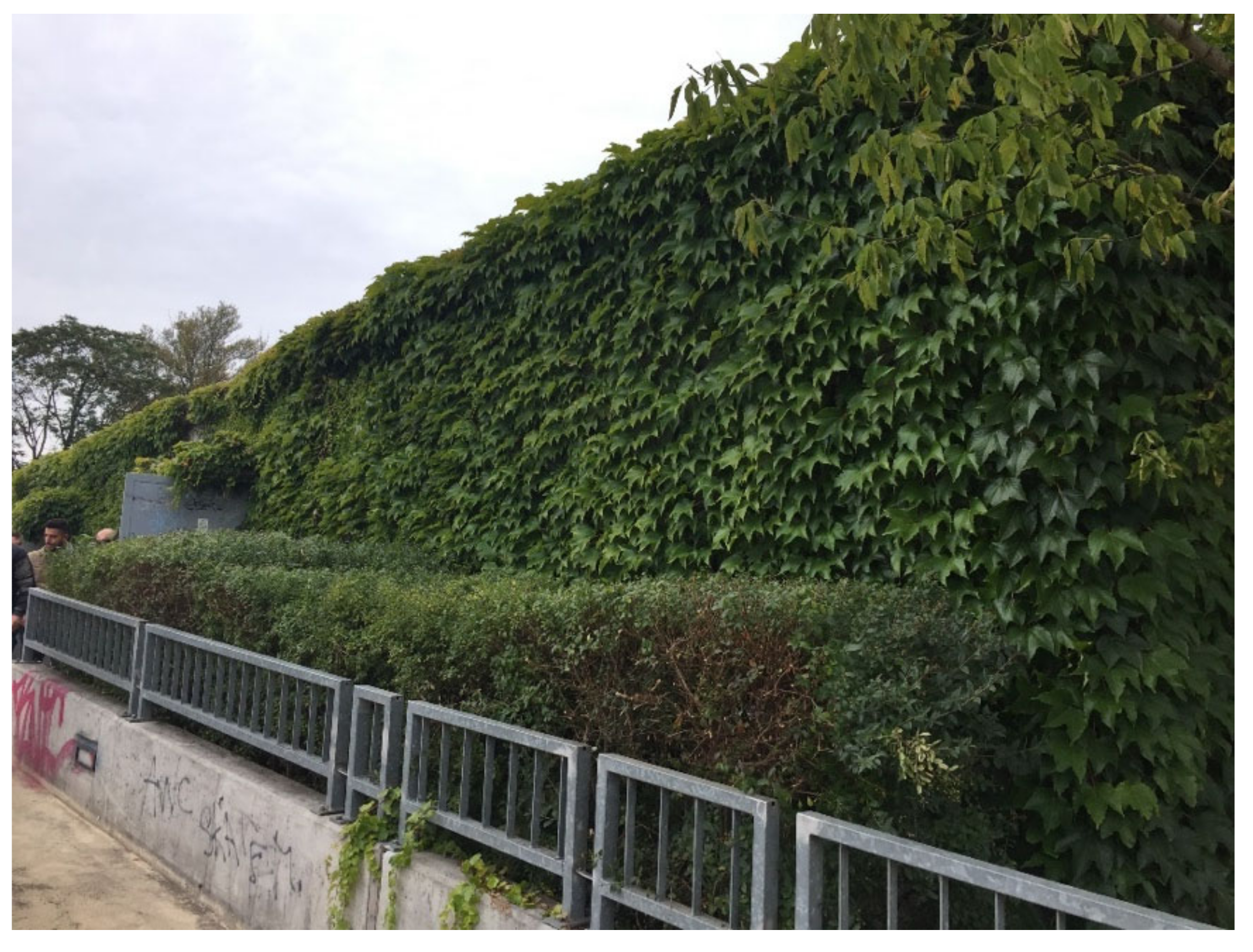
Funding

This research received no external funding.

Conflicts of Interest

The authors declare no conflict of interest.

References

  1. Safikhani, T.; Abdullah, A.M.; Ossen, D.R.; Baharvand, M. A Review of Energy Characteristic of Vertical Greenery Systems. Renew. Sustain. Energy Rev. 2014, 40, 450–462. [Google Scholar] [CrossRef]
  2. Loh, S. Living Walls—A Way to Green the Built Environment; Environment Design Guide: Canberra, Australia, 2008; pp. 1–7. Available online: https://www.jstor.org/stable/26149051 (accessed on 13 November 2022).
  3. Köhler, M. Green Façades—A View Back and Some Visions. Urban Ecosyst. 2008, 11, 423–436. [Google Scholar] [CrossRef]
  4. Riley, B. The State of the Art of Living Walls: Lessons Learned. Build. Environ. 2017, 114, 219–232. [Google Scholar] [CrossRef]
  5. Malys, L.; Musy, M.; Inard, C. A Hydrothermal Model to Assess the Impact of Green Walls on Urban Microclimate and Building Energy Consumption. Build. Environ. 2014, 73, 187–197. [Google Scholar] [CrossRef]
  6. Scarpa, M.; Mazzali, U.; Peron, F. Modeling the Energy Performance of Living Walls: Validation against Field Measurements in Temperate Climate. Energy Build. 2014, 79, 155–163. [Google Scholar] [CrossRef]
  7. He, Y.; Yu, H.; Ozaki, A.; Dong, N.; Zheng, S. An Investigation on the Thermal and Energy Performance of Living Wall System in Shanghai Area. Energy Build. 2017, 140, 324–335. [Google Scholar] [CrossRef]
  8. Razzaghmanesh, M.; Razzaghmanesh, M. Thermal Performance Investigation of a Living Wall in a Dry Climate of Australia. Build. Environ. 2017, 112, 45–62. [Google Scholar] [CrossRef]
  9. Sunakorn, P.; Yimprayoon, C. Thermal Performance of Biofaçade with Natural Ventilation in the Tropical Climate. Procedia Eng. 2011, 21, 34–41. [Google Scholar] [CrossRef]
  10. Charoenkit, S.; Yiemwattana, S. Role of Specific Plant Characteristics on Thermal and Carbon Sequestration Properties of Living Walls in Tropical Climate. Build. Environ. 2017, 115, 67–79. [Google Scholar] [CrossRef]
  11. Fowdar, H.S.; Hatt, B.E.; Breen, P.; Cook, P.L.M.; Deletic, A. Designing Living Walls for Greywater Treatment. Water Res. 2017, 110, 218–232. [Google Scholar] [CrossRef]
  12. Prodanovic, V.; Zhang, K.; Hatt, B.; McCarthy, D.; Deletic, A. Optimisation of Lightweight Green Wall Media for Greywater Treatment and Reuse. Build. Environ. 2018, 131, 99–107. [Google Scholar] [CrossRef]
  13. Prodanovic, V.; McCarthy, D.; Hatt, B.; Deletic, A. Designing Green Walls for Greywater Treatment: The Role of Plants and Operational Factors on Nutrient Removal. Ecol. Eng. 2019, 130, 184–195. [Google Scholar] [CrossRef]
  14. Jin, Z.; Xie, X.; Zhou, J.; Bei, K.; Zhang, Y.; Huang, X.; Zhao, M.; Kong, H.; Zheng, X. Blackwater Treatment Using Vertical Greening: Efficiency and Microbial Community Structure. Bioresour. Technol. 2018, 249, 175–181. [Google Scholar] [CrossRef] [PubMed]
  15. Wong, N.H.; Kwang Tan, A.Y.; Tan, P.Y.; Chiang, K.; Wong, N.C. Acoustics Evaluation of Vertical Greenery Systems for Building Walls. Build. Environ. 2010, 45, 411–420. [Google Scholar] [CrossRef]
  16. Irga, P.J.; Braun, J.T.; Douglas, A.N.J.; Pettit, T.; Fujiwara, S.; Burchett, M.D.; Torpy, F.R. The Distribution of Green Walls and Green Roofs throughout Australia: Do Policy Instruments Influence the Frequency of Projects? Urban For. Urban Green 2017, 24, 164–174. [Google Scholar] [CrossRef]
  17. Ottelé, M.; Perini, K.; Fraaij, A.L.A.; Haas, E.M.; Raiteri, R. Comparative Life Cycle Analysis for Green Façades and Living Wall Systems. Energy Build. 2011, 43, 3419–3429. [Google Scholar] [CrossRef]
  18. Chew, M.Y.L.; Conejos, S. Developing a Green Maintainability Framework for Green Walls in Singapore. Struct. Surv. 2016, 34, 379–406. [Google Scholar] [CrossRef]
  19. Ascione, F. Energy Conservation and Renewable Technologies for Buildings to Face the Impact of the Climate Change and Minimize the Use of Cooling. Sol. Energy 2017, 154, 34–100. [Google Scholar] [CrossRef]
  20. Dunnett, N.; Kingsbury, N. Planting Green Roofs and Living Walls, 2nd ed.; Timber Press Inc: Portland, OR, USA, 2008; ISBN 978-0-88192-911-9. [Google Scholar]
  21. Perkins, M.; Joyce, D. Living Wall and Green Roof Plants for Australia; Rural Industries Research and Development Corporation: Canberra, Australia, 2012. [Google Scholar]
  22. Cameron, R.W.; Taylor, J.E.; Emmett, M.R. What’s ‘Cool’ in the World of Green Façades? How Plant Choice Influences the Cooling Properties of Green Walls. Build. Environ. 2014, 73, 198–207. [Google Scholar] [CrossRef]
  23. Mårtensson, L.-M.; Fransson, A.-M.; Emilsson, T. Exploring the Use of Edible and Evergreen Perennials in Living Wall Systems in the Scandinavian Climate. Urban For. Urban Green. 2016, 15, 84–88. [Google Scholar] [CrossRef]
  24. Jørgensen, L.; Dresbøll, D.B.; Thorup-Kristensen, K. Root Growth of Perennials in Vertical Growing Media for Use in Green Walls. Sci. Hortic. 2014, 166, 31–41. [Google Scholar] [CrossRef]
  25. Manso, M.; Castro-Gomes, J. Green Wall Systems: A Review of Their Characteristics. Renew. Sustain. Energy Rev. 2015, 41, 863–871. [Google Scholar] [CrossRef]
  26. Whittinghill, L.J.; Rowe, D.B. Salt Tolerance of Common Green Roof and Green Wall Plants. Urban Ecosyst. 2011, 14, 783–794. [Google Scholar] [CrossRef]
  27. Bustami, R.; Brien, C.; Ward, J.; Beecham, S.; Rawlings, R. A Statistically Rigorous Approach to Experimental Design of Vertical Living Walls for Green Buildings. Urban Sci. 2019, 3, 71. [Google Scholar] [CrossRef]
  28. Perini, K.; Ottelé, M.; Haas, E.M.; Raiteri, R. Vertical Greening Systems, a Process Tree for Green Façades and Living Walls. Urban Ecosyst. 2013, 16, 265–277. [Google Scholar] [CrossRef]
  29. Bustami, R.A.; Belusko, M.; Ward, J.; Beecham, S. Vertical Greenery Systems: A Systematic Review of Research Trends. Build. Environ. 2018, 146, 226–237. [Google Scholar] [CrossRef]
  30. Bustami, R.A.; Beecham, S.; Hopeward, J. Evaporative Cooling Effect of Water Sensitive Urban Design: Comparing a Living Wall with a Porous Concrete Pavement System. Water 2022, 14, 3759. [Google Scholar] [CrossRef]
  31. Farrell, C.; Mitchell, R.E.; Szota, C.; Rayner, J.P.; Williams, N.S.G. Green Roofs for Hot and Dry Climates: Interacting Effects of Plant Water Use, Succulence and Substrate. Ecol. Eng. 2012, 49, 270–276. [Google Scholar] [CrossRef]
  32. Pérez-Harguindeguy, N.; Díaz, S.; Lavorel, S.; Poorter, H.; Jaureguiberry, P.; Bret-Harte, M.S.S.; Cornwell, W.K.K.; Craine, J.M.M.; Gurvich, D.E.E.; Urcelay, C.; et al. New Handbook for Standardized Measurment of Plant Functional Traits Worldwide. Aust. J. Bot. 2013, 61, 167–234. [Google Scholar] [CrossRef]
  33. Liu, C.; Wang, Y.; Pan, K.; Jin, Y.; Li, W.; Zhang, L. Effects of Phosphorus Application on Photosynthetic Carbon and Nitrogen Metabolism, Water Use Efficiency and Growth of Dwarf Bamboo (Fargesia Rufa) Subjected to Water Deficit. Plant Physiol. Biochem. 2015, 96, 20–28. [Google Scholar] [CrossRef]
  34. Butler, D.G.; Cullis, B.R.; Gilmour, A.R.; Gogel, B.J. Analysis of Mixed Models for S Language Environments: ASReml-R Reference Manual; DPI Publications: Brisbane, QL, Australia, 2009. [Google Scholar]
  35. Brien, C.J. asremlplus: Augments the use of ASReml-R in Fitting Mixed Models, 4.0-9. 2017. Available online: https://cran.at.r-project.org/package=asremlPlus (accessed on 10 April 2018).
  36. R Development Core Team. R: A Language and Environment for Statistical Computing; R Foundation for Statistical Computing: Vienna, Austria, 2019; Available online: https://www.r-project.org (accessed on 9 March 2019).
  37. Bachok, N. Univariable Analyses, 1st ed.; Pustaka Aman Press Sdn Bhd: Kota Bharu, Malaysia, 2013; p. 114. ISBN 978-967-10386-3-5. [Google Scholar]
  38. George, D.; Mallery, M. SPSS for Windows Step by Step: A Simple Guide and Reference, 10th ed.; Pearson: Boston, MA, USA, 2010; p. 63. ISBN 978-020-57556-1-5. [Google Scholar]
  39. Karuthan, C.; Choo, W.Y. Statistical Analysis Using SPSS, 3rd ed.; Pearson: Kuala Lumpur, Malaysia, 2016. [Google Scholar]
  40. Kim, H.Y. Statistical notes for clinical researchers: Chi-squared test and Fisher’s exact test. Restor. Dent. Endod. 2017, 42, 152–155. [Google Scholar] [CrossRef] [PubMed]
  41. Kroonenberg, P.M.; Verbeek, A. The Tale of Cochran’s Rule: My Contingency Table has so Many Expected Values Smaller than 5, What Am I to Do? Am. Stat. 2018, 72, 175–183. [Google Scholar] [CrossRef]
  42. Serra, V.; Bianco, L.; Candelari, E.; Giordano, R.; Montacchini, E.; Tedesco, S.; Larcher, F.; Schiavi, A. A Novel Vertical Greenery Module System for Building Envelopes: The Results and Outcomes of a Multidisciplinary Research Project. Energy Build. 2017, 146, 333–352. [Google Scholar] [CrossRef]
  43. Mårtensson, L.-M.; Wuolo, A.; Fransson, A.-M.; Emilsson, T. Plant Performance in Living Wall Systems in the Scandinavian Climate. Ecol. Eng. 2014, 71, 610–614. [Google Scholar] [CrossRef]
  44. Jørgensen, L.; Dresbøll, D.B.; Thorup-Kristensen, K. Spatial Root Distribution of Plants Growing in Vertical Media for Use in Living Walls. Plant Soil 2014, 380, 231–248. [Google Scholar] [CrossRef]
  45. Bureau of Meteorology. Adelaide in Summer 2018. Available online: http://www.bom.gov.au/climate/current/season/sa/archive/201802.adelaide.shtml (accessed on 5 July 2019).
  46. Bureau of Meteorology. Adelaide in 2018 . Available online: http://www.bom.gov.au/climate/current/annual/sa/archive/2018.adelaide.shtml (accessed on 5 July 2019).
Figure 1. An example of a green façade.
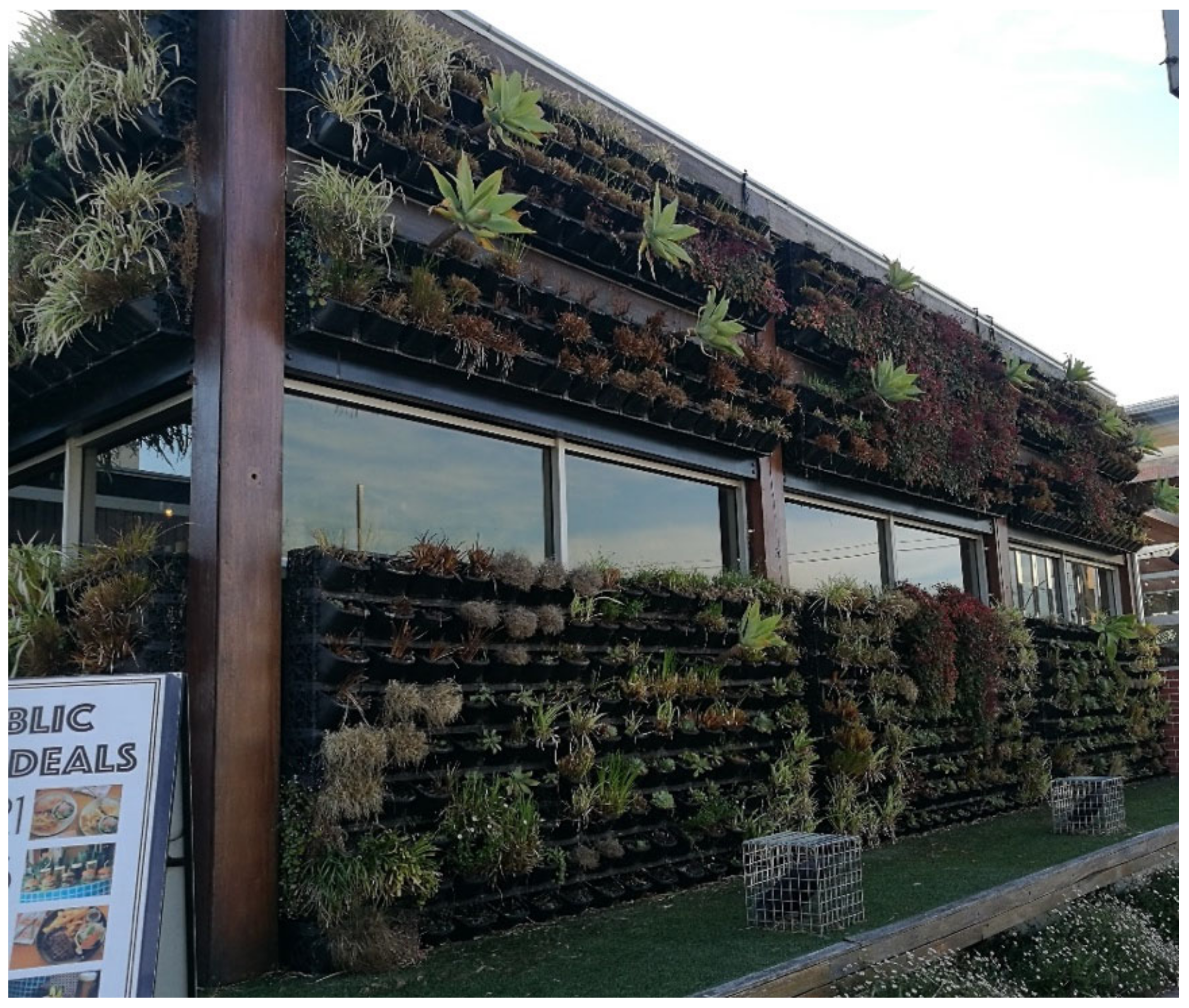
Environments 10 00026 g001
Figure 2. A living wall in Adelaide, South Australia.
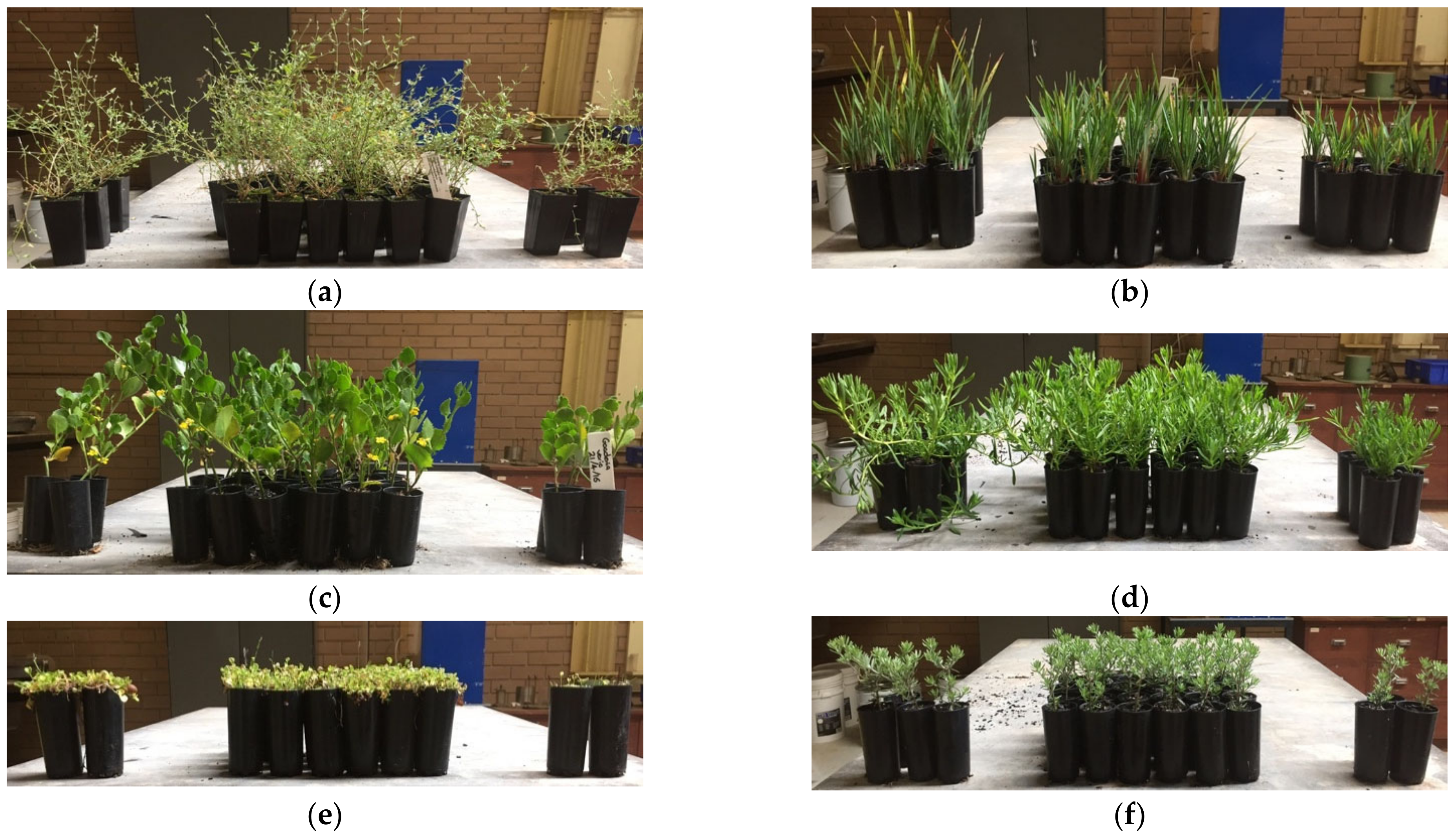
Environments 10 00026 g002
Figure 3. Plants in tube stocks sorted according to height before being planted into living wall pots. The species were: (a) EN: E. nutans; (b) DR: D. revoluta; (c) GV: G. varia; (d) MP: M. parvifolium; (e) TT: D. repens; and (f) WF: W. fruticosa.
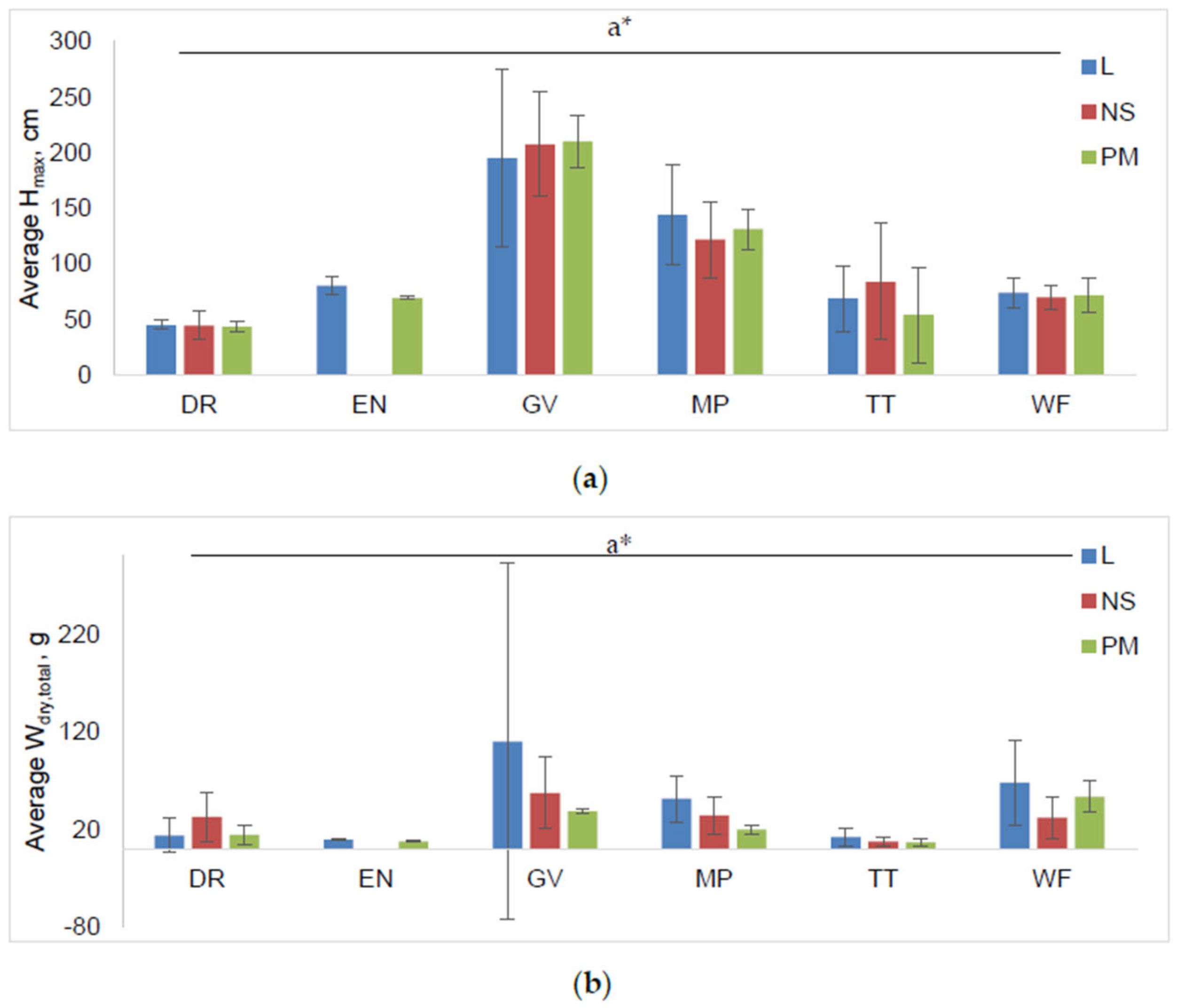
Environments 10 00026 g003
Figure 4. (a) Average maximum height (in cm) and (b) average total dry weight (in g), for plants that survived the entire experiment, according to their substrate types. The error bars denote the standard deviation. L: Loam, NS: Native soil, PM: Potting mix, DR: D. revoluta, EN: E. nutans, GV: G. varia, MP: M. parvifolium, TT: D. repens, WF: W. fruticosa, Avg: Average, Hmax: maximum height, Wdry, total: Total dry weight, a: Kruskal–Wallis test, *: p < 0.05.
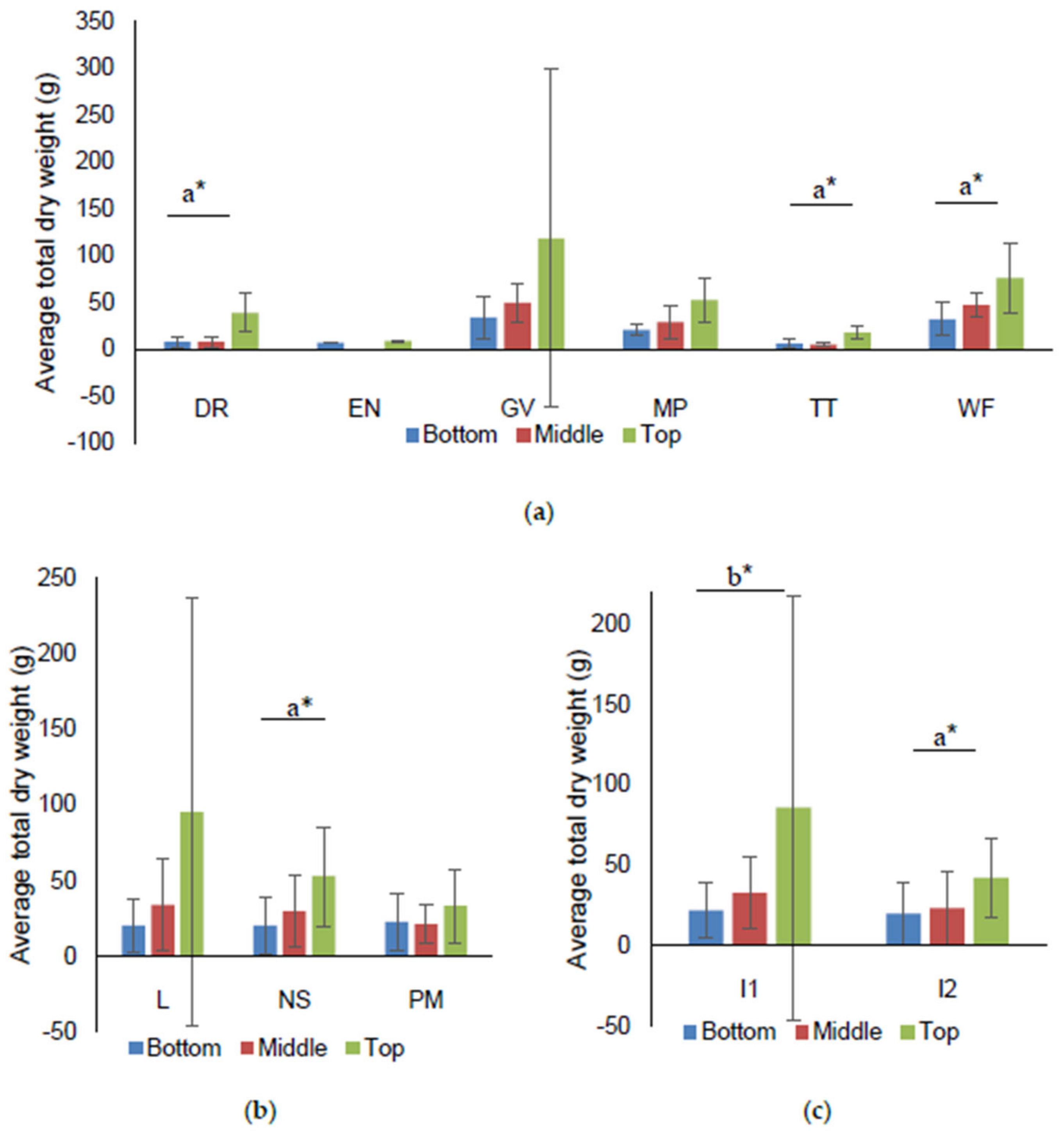
Environments 10 00026 g004
Figure 5. Average total dry weight of 102 plants at harvest (in g), according to their row locations with standard deviations shown in error bars, for all (a) plant species, (b) substrates, and (c) irrigation. DR: D. revoluta, EN: E. nutans, GV: G. varia, MP: M. parvifolium, TT: D. repens, WF: W. fruticose, L: loam, NS: native soil, PM: potting mix, I1: irrigation 1, I2: irrigation 2, a: ANOVA, b: Kruskal–Wallis, *: p < 0.05.
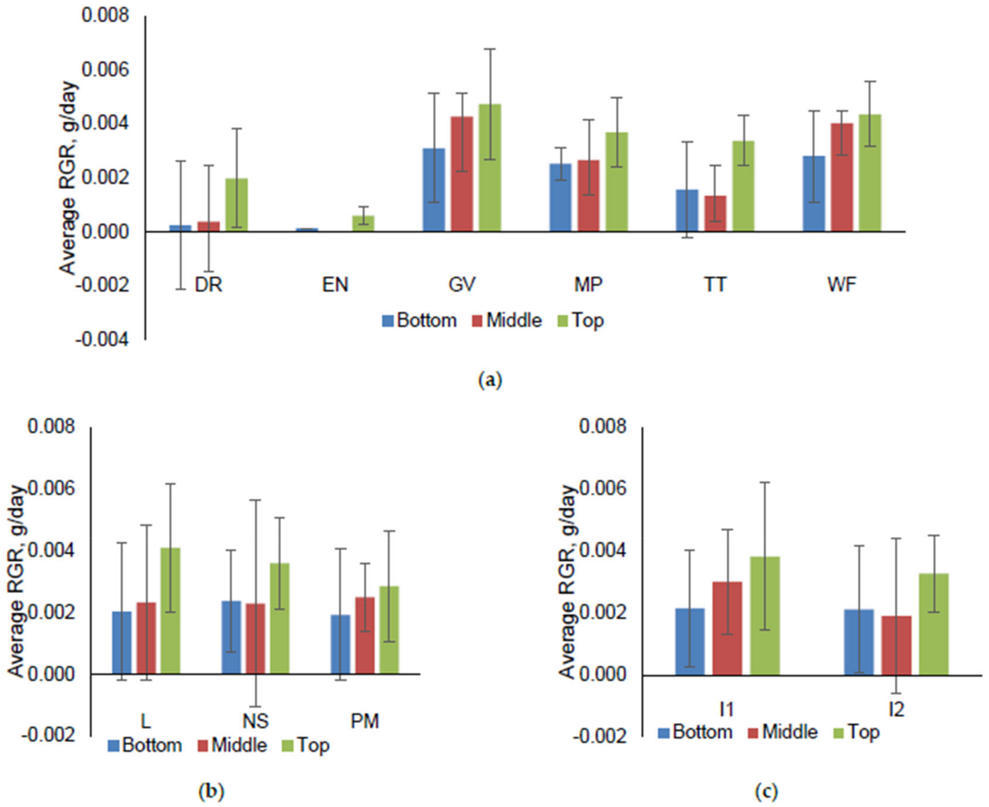
Environments 10 00026 g005
Figure 6. Average Relative growth rate (RGR) in g/day with standard deviations shown in error bars for all (a) plants, (b) substrates and (c) irrigation according to height sections on the living wall. L: loam, NS: native soil, PM: potting mix, I1: irrigation 1, I2: irrigation 2, DR: D. revoluta, EN: E. nutans, GV: G. varia, MP: M. parvifolium, TT: D. repens, WF: W. fruticosa.
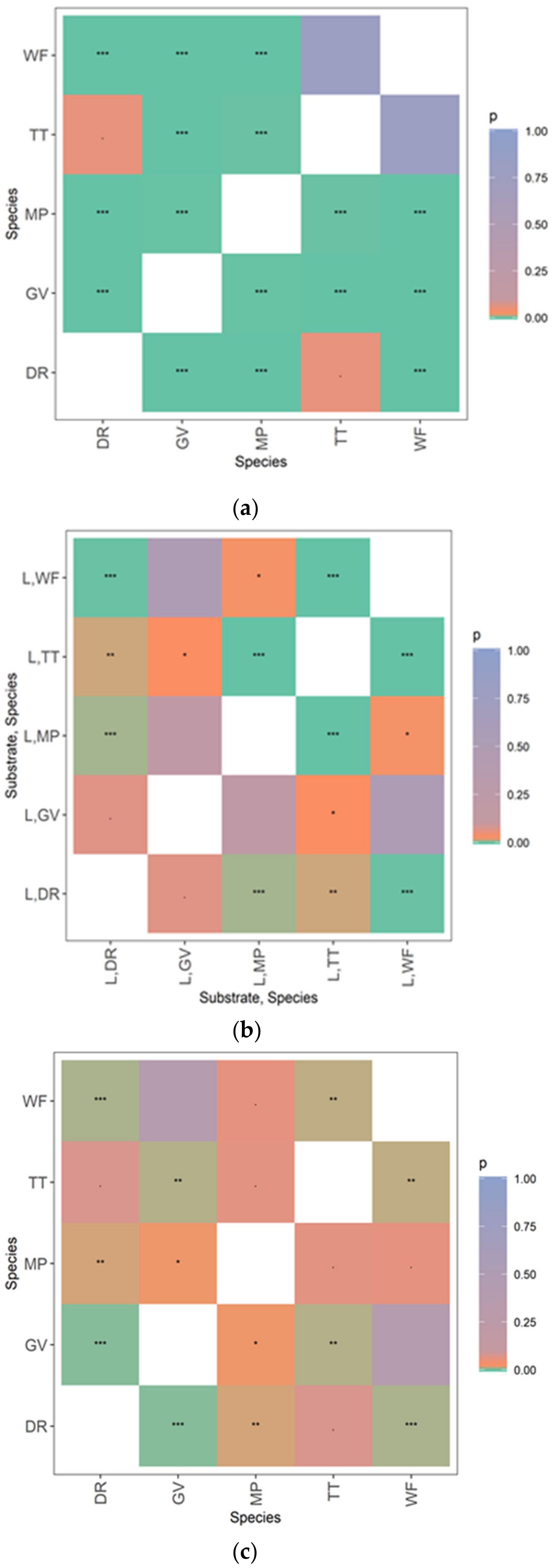
Environments 10 00026 g006
Figure 7. Heat maps of the p-value for predictions on (a) maximum height between species, (b) total dry weight between species and substrates and (c) relative growth rate (RGR) between species.
Environments 10 00026 g007
Table 1. Plant-substrate-irrigation arrangement on the living wall.
Column1 2 3 4 5 6 7 8 9 10 11 12
Row
12EN-PM-I1 TT-PM-I1 WF-PM-I2 EN-L-I1 MP-NS-I2 DR-NS-I1 WF-L-I1 MP-L-I2 DR-L-I2 EN-L-I2 GV-PM-I1 DR-NS-I2
11 GV-NS-I2 GV-NS-I1 WF-NS-I2 MP-L-I1 WF-L-I2 WF-PM-I2 TT-L-I1 EN-NS-I1 DR-PM-I2 DR-L-I2 WF-PM-I1 DR-NS-I1
10 TT-PM-I2 GV-PM-I2 EN-PM-I2 DR-PM-I1 EN-L-I1 MP-L-I1 MP-NS-I1 WF-NS-I2 TT-L-I2 GV-L-I1 DR-NS-I2 GV-NS-I1
9 MP-NS-I2 EN-PM-I1 TT-L-I1 WF-L-I2 TT-NS-I1 GV-L-I2 MP-PM-I1 WF-L-I1 GV-PM-I2 EN-NS-I1 EN-L-I2 MP-L-I1
8 DR-NS-I1 WF-NS-I2 DR-L-I1 MP-NS-I1 GV-L-I2 EN-PM-I1 EN-NS-I2 DR-PM-I2 GV-L-I1 TT-PM-I2 GV-NS-I2 TT-PM-I1
7 MP-L-I2 EN-L-I1 GV-PM-I1 TT-NS-I2 EN-NS-I2 TT-PM-I1 WF-NS-I2 TT-PM-I2 MP-PM-I1 DR-PM-I2 DR-L-I1 EN-L-I2
6 MP-L-I1 DR-NS-I1 TT-NS-I2 GV-NS-I1 MP-PM-I1 DR-PM-I2 GV-NS-I2 GV-L-I2 MP-PM-I2 EN-L-I1 TT-L-I2 WF-PM-I1
5 EN-NS-I1 DR-L-I1 MP-PM-I2 DR-NS-I2 WF-PM-I1 DR-L-I2 GV-PM-I1 TT-NS-I1 EN-NS-I2 GV-PM-I2 MP-PM-I1 MP-L-I2
4 WF-NS-I1 TT-NS-I2 WF-L-I1 WF-PM-I1 DR-PM-I1 WF-L-I2 GV-L-I1 EN-PM-I2 EN-PM-I1 MP-NS-I2 TT-L-I1 GV-NS-I2
3 WF-PM-I2 TT-L-I2 EN-NS-I1 TT-L-I1 MP-NS-I1 TT-PM-I2 MP-L-I2 WF-NS-I1 DR-L-I1 DR-PM-I1 MP-NS-I2 EN-NS-I2
2 DR-PM-I1 WF-L-I2 GV-L-I1 EN-PM-I2 MP-PM-I2 WF-NS-I1 WF-PM-I2 DR-L-I2 MP-NS-I1 TT-NS-I1 TT-NS-I2 GV-L-I2
1 EN-L-I2 DR-NS-I2 TT-L-I2 GV-PM-I2 GV-PM-I1 TT-NS-I1 EN-PM-I2 GV-NS-I1 WF-L-I1 WF-NS-I1 TT-PM-I1 MP-PM-I2
Plant species (4 replicates): DR: D. revoluta, EN: E. nutans, GV: G. varia, MP: M. parvifolium, TT: D. repens, WF: W. fruticosa; Soil substrate (4 replicates): L: organic sandy loam; NS: native soil; PM: potting mix; Irrigation (4 replicates): I1: Irrigation 1 (2 min @ 4 L/h); I2: Irrigation 2 (3 min @ 2 L/h).
Table 2. Measurements and observations of the living wall plants with apparatus used for each procedure.
Measurements and ObservationsApparatus
At the start of the experiment
1.Sample plant total length (mm)Measuring tape
2.Sample plant biomass (g)Oven and weighing scale
During the experiment
1.Above ground height or length (mm)Measuring tape
2.Above ground width (mm)Measuring tape
3. Flower countVisual
4.Shaded, crowded or tangledVisual
5.Plant survival and healthVisual
7.Pests or other faunaVisual
At harvest
1.Root and shoot height or length (mm)Measuring tape
2.Root and shoot biomass (g)Oven and weighing scale
3.Flower countVisual
4.Plant survival and healthVisual
5.Pests or other faunaVisual
Table 3. Plant health classification and percentage range, visually assessed during the experiment and at harvest.
Plant Health ClassificationPercentage of Green and Healthy Plant Foliage
Unhealthy0 to 30%
Moderately healthy31 to 60%
Healthy61 to 90%
Very healthy91 to 100%
Table 4. Average outlet water volume (in mL) collected per irrigation session for the bottom, middle and top living wall pot rows, according to their substrate types.
L (mL)NS (mL)PM (mL)
Bottom rows (Rows 1 to 4)66.246.467.9
Middle rows (Rows 5 to 8)38.939.138.3
Top rows (Rows 9 to 12)18.617.330.7
Living wall average41.438.250.6
L: loam, N: native soil, PM: potting mix.
Table 5. Number of surviving specimens according to plant species, substrates and irrigation regimes.
Pl.LSubtotalNSSubtotalPMSubtotalTotal
I1I2I1I2I1I2
DR23513423514
EN1120001124
GV44834743722
MP44843743722
TT24624634719
WF34743743721
162036141731181735102
Pl.: Plant species, L: Loam, NS: Native soil, PM: Potting mix, DR: D. revoluta, EN: E. nutans, GV: G. varia, MP: M. parvifolium, TT: D. repens, WF: W. fruticosa, I1: Irrigation 1, I2: Irrigation 2.
Table 6. Statistical analysis of survival rate.
A) Between species, including analysis within substrate types and within irrigation regimes
ParametersNumber of Plants in
DRENGVMPTTWFp
YNYNYNYNYNYN
Between species14104202222221952130.000 a*
Within substrates between speciesL5326808062710.004 a*
NS4408717162710.000 a*
PM5326717171710.022 a*
Within irrigation between speciesI157210111120751110.000 a*
I2932101111021201020.000 a*
B) Between substrates, including analysis within plant species and within irrigation regimes
ParametersNumber of Plants in
LNSPMp
YNYNYN
Between substrates3612311725130.494 a
Within species between substratesDR5344531.000 a
EN2608260.494 a
GV8071711.000 a
MP8071711.000 a
TT6262711.000 a
WF7171711.000 a
Within irrigation between substratesI116814101860.472 a
I22041771770.513 a
C) Between irrigation regimes, including analysis within plant species and within substrate types
ParametersNumber of Plants in I1Number of Plants in I2p
YNYN
Between irrigations482454180.271 a
Within species between irrigationsDR57930.098 a
EN2102101.000 b
GV1111111.000 b
MP1201020.478 b
TT751200.037 b*
WF1111021.000 b
Within substrate between irrigationsL1682040.318 b
NS14101770.547 b
PM1861771.000 b
L: Loam, NS: Native soil, PM: Potting mix, DR: D. revoluta, EN: E. nutans, GV: G. varia, MP: M. parvifolium, TT: D. repens, WF: W. fruticosa, I1: Irrigation 1, I2: Irrigation 2, Y: Plants survived; N: Plants did not survive; a Chi-square; b Fisher’s Exact test; * p < 0.05.
Table 7. Analysis of means for average plant health (in %) for plant species, including analysis within substrate types and within irrigation regimes.
ParametersAverage Plant Health and SD in (%)p
DRENGVMPTTWF
Species76.4 ± 15.482.5 ± 17.193.9 ± 8.474.8 ± 11.889.7 ± 7.098.8 ± 3.80.000 a*
Within substrates between speciesL77.0 ± 13.080.0 ± 28.396.9 ± 3.778.1 ± 10.087.5 ± 5.298.6 ± 3.80.001 b*
NS83.8 ± 16.0n/a90.7 ± 14.073.6 ± 14.189.2 ± 9.297.9 ± 5.70.013 a*
PM70.0 ± 17.385.0 ± 7.193.6 ± 3.872.1 ± 12.292.1 ± 6.4100.0 ± 0.00.001 b*
Within irrigation between speciesI179.0 ± 16.075.0 ± 21.294.5 ± 4.270.4 ± 9.291.4 ± 8.098.6 ± 4.50.000 a*
I275.0 ± 15.890.0 ± 14.193.2 ± 11.580.0 ± 12.988.8 ± 6.499.0 ± 3.20.000 a*
L: Loam, NS: Native soil, PM: Potting mix, DR: D. revoluta, EN: E. nutans, GV: G. varia, MP: M. parvifolium, TT: D. repens, WF: W. fruticosa, I1: Irrigation 1, I2: Irrigation 2, n/a: not available, a Kruskal–Wallis, b Anova, * p < 0.05.
Table 8. Analysis of means for RGR for plant species, including analysis within substrate types and within irrigation regimes.
ParametersAverage RGR and SD (in g/day)p
DRENGVMPTTWF
Between species0.0005 ± 0.00250.0005 ± 0.00040.0041 ± 0.00180.0030 ± 0.00130.0019 ± 0.00160.0036 ± 0.00150.000 a*
Within substrates L0.0005 ± 0.00250.0005 ± 0.00040.0041 ± 0.00180.0030 ± 0.00130.0019 ± 0.00160.0036 ± 0.00150.000 a*
NS−0.0001 ± 0.00220.0008 ± 0.00030.0041 ± 0.00280.0036 ± 0.00170.0025 ± 0.00140.0040 ± 0.00170.008 a*
PM0.0006 ± 0.0041n/a0.0044 ± 0.00120.0030 ± 0.00130.0020 ± 0.00160.0026 ± 0.00180.080 b
Within irrigations I10.0010 ± 0.00150.0002 ± 0.00010.0039 ± 0.00020.0023 ± 0.00040.0012 ± 0.00170.0041 ± 0.00040.000 b*
I20.0005 ± 0.00170.0006 ± 0.00050.0044 ± 0.00230.0034 ± 0.00120.0019 ± 0.00200.0034 ± 0.00170.001 a*
L: Loam, NS: Native soil, PM: Potting mix, DR: D. revoluta, EN: E. nutans, GV: G. varia, MP: M. parvifolium, TT: D. repens, WF: W. fruticosa, I1: Irrigation 1, I2: Irrigation 2, n/a: not available, a Anova, b Kruskal–Wallis, * p < 0.05.
Disclaimer/Publisher’s Note: The statements, opinions and data contained in all publications are solely those of the individual author(s) and contributor(s) and not of MDPI and/or the editor(s). MDPI and/or the editor(s) disclaim responsibility for any injury to people or property resulting from any ideas, methods, instructions or products referred to in the content.

