Article

Intelligent Fault Prognosis Method Based on Stacked Autoencoder and Continuous Deep Belief Network

1
Department of Integrated Technology and Control Engineering, School of Aeronautics, Northwestern Polytechnical University, Xi’an 710072, China
2
Aeronautical Radio Electronics Research Institute, Shanghai 200233, China
*
Author to whom correspondence should be addressed.
These authors contributed equally to this work.
Actuators 2023, 12(3), 117; https://doi.org/10.3390/act12030117
Submission received: 1 February 2023 / Revised: 27 February 2023 / Accepted: 2 March 2023 / Published: 9 March 2023

Abstract

:
Mechanical fault prediction is one of the main problems in condition-based maintenance, and its purpose is to predict the future working status of the machine based on the collected status information of the machine. However, on one hand, the model health indices based on the information collected by the sensors will directly affect the evaluation results of the system. On the other hand, because the model health index is a continuous time series, the effect of feature learning on continuous data also affects the results of fault prognosis. This paper makes full use of the autonomous information fusion capability of the stacked autoencoder and the strong feature learning capability of continuous deep belief networks for continuous data, and proposes a novel fault prognosis method. Firstly, a stacked autoencoder is used to construct the model health index through the feature learning and information fusion of the vibration signals collected by the sensors. To solve the local fluctuations in the health indices, the exponentially weighted moving average method is used to smooth the index data to reduce the impact of noise. Then, a continuous deep belief network is used to perform feature learning on the constructed health index to predict future performance changes in the model. Finally, a fault prognosis experiment based on bearing data was performed. The experimental results show that the method combines the advantages of stacked autoencoders and continuous deep belief networks, and has a lower prediction error than traditional intelligent fault prognosis methods.

1. Introduction

When machinery is rotated to achieve motion conversion, the bearing is the most critical component, and the most prone to fault, in the entire transmission system. According to statistics, 30% of machinery faults are caused by bearings [1]. Fault prognosis is gaining traction because of the potential value in reducing loss to property by predicting the future performance of components.
At present, fault prognosis methods are mainly divided into two major directions: model-based fault prognosis and data-driven fault prognosis [2]. The model-based fault prognosis method assumes that an accurate mathematical model of the object system can be constructed [3]. The performance of the part is evaluated by calculation of functional damage, and the remaining life of the part is evaluated by building physical and simulation models [4]. Janjarasjitt et al. constructed a mathematical model that characterizes the operating state of a bearing by using partially correlated integrals [5]. Lei et al. used algebraic equations to construct a planetary gearbox vibration signal model for gearbox failure prediction [6]. Huang et al. extracted fault feature information from the system’s operating state and built a fault state model using the Kalman rate and an expert system for fault prognosis [7]. Du et al. combined the advantages of strong tracking square root Kalman filters and autoregressive models to build a future measurement state prediction model [8]. Lin et al. combined the concept of fuzzy posted progress in fuzzy mathematics with particle filtering to realize the fault prognosis of a three-tank water tank system and a planetary gear system [9]. Although the model-based method can achieve fault prognosis, it has two disadvantages that cannot be ignored: (1) There is a strong dependence on the model. The model built will directly affect the effect of fault prognosis, and it is often difficult to build accurate mathematical models for complex dynamic systems. (2) The model generalization is poor. The built model needs to consider various working conditions and operating states of the predicted object. The generality of the physical model is usually poor, causing unnecessary waste of human and financial resources.
The data-driven fault prognosis method is based on historical data and uses data mining to find the performance change characteristics of the model to achieve fault prognosis [10]. Marco et al. extensively reviewed the latest developments in non-destructive techniques [11]. Zhang et al. established a chaotic time series of oil chromatography data by introducing chaos theory, and used the Lyapunov exponent method to predict the gas volume trend in oil [12]. Peng et al. used the moving average model to predict the dissolved gas content in transformer oil [13]. Yan et al. established a system performance degradation model and used the auto-regression and moving average model to predict the remaining useful life of the system [14]. Rigamonti et al. used an integrated echo state network for fault prognosis of industrial components [15]. Xu et al. used a long short-term memory model and principal component analysis to realize shield fault prognosis [16]. Li et al. used kernel principal component analysis and the hierarchically gated recursive unit network to predict the health status of bearings [17]. Cecilia Surace et al. proposed an instantaneous spectral entropy and continuous wavelet transform for anomaly detection and fault diagnosis using gearbox vibration time histories [18]. Zhou et al. combined the advantages of principal component analysis and automatic encoders to successfully implement early monitoring and prognosis of slowly varying fault signals [19].
Although the data-driven fault prognosis method removes the dependence on models, there are still three shortcomings: (1) The health index that characterizes the changes in model performance directly affects the effectiveness of fault prediction. Machine learning methods such as principal component analysis (PCA) and locally linear embedding (LLE) have limited feature learning capabilities and cannot fully learn model performance change information. (2) The disturbance of the vibration signal noise collected by the sensor will cause random disturbances in the constructed health index, which will affect the fault prognosis effect. (3) The constructed health index is a continuous time series. Traditional intelligent prediction methods have limited ability to learn continuous data features.
In order to solve the above problems, this paper proposes an intelligent fault prognosis method based on stacked autoencoders and continuous deep belief networks. Our work is summarized as follows:
(1)
In order to construct a health index that can accurately represent the change in model performance, this paper makes full use of the powerful feature learning capabilities and information fusion capabilities of stacked autoencoders.
(2)
In order to solve the problem of local random interference in the health index, this paper uses the exponential weighted moving average method to smooth the health index. It can integrate historical information with current information to reduce the impact of noise.
(3)
In order to capture the feature information of the continuous time series, this paper makes full use of the continuous deep belief network’s powerful feature learning ability and fault prognosis ability for continuous data.
(4)
In order to verify the prediction effect of the fault prognosis method in this paper, a comparative experiment on fault prognosis is carried out using intelligent maintenance systems (IMS) bearing data as an example.
The rest of the paper is arranged as follows: in Section 2, we briefly introduce the stacked autoencoder and deep belief network; in Section 3, we introduce the proposed fault prognosis method in detail; in Section 4, we conduct experiments to verify the effectiveness of the proposed method; and Section 5 is the conclusion.

2. Basic Theories of Stacked Autoencoder and Deep Belief Network

2.1. Stacked Autoencoder

Autoencoders are the basic unit of a stacked autoencoder’s composition and function. As shown in Figure 1, the autoencoder is a three-layer neural network consisting of a visible layer, a hidden layer, and an output layer. In essence, an autoencoder can be divided into two parts, namely an encoder and a decoder. A stacked autoencoder, as shown in Figure 2, is a deep learning model composed of multiple autoencoders, where the output of each hidden layer is connected to the input of the successive hidden layer. After all the hidden layers are trained, a backpropagation algorithm (BP) is used to minimize the cost and update the weights with a labeled training set to achieve fine-tuning.
First of all, we will describe the encoding part. The mapping of high-dimensional data from the input layer to the hidden layer is the feature learning and information fusion of the model.
y = sigmoid W x + b
where W represents the weight matrix of the encoding part, b represents the offset vector of the encoding part, and x represents the input data.
In the decoding, the mapping from the hidden layer to the output layer is regarded as restoring the learned deep feature information to the original state.
y = sigmoid W h + b
where W represents the weight matrix of the decoding part, b represents the offset vector of the decoding part, and h represents the learned deep feature information.
Since the structure of the input and output is the same, the training process of the autoencoder is a self-supervised learning process. By continuously reducing the error between the input data and the output data, the training of the autoencoder is realized. This article uses the mean square error cost function as a measure of model training. The mean square error cost function is defined as follows:
E = 1 S j = 1 S 1 2 i = 1 n x i j y i j 2

2.2. Deep Belief Network

A deep belief network (DBN) is a deep learning model based on data probability distribution proposed by Hinton in 2006 [20]. Deep belief network consists of multiple restricted Boltzmann machines (RBMs) and a BP neural network. RBMs are the basic unit of DBNs that implement feature extraction and data mining.
As shown in Figure 3, an RBM is a two-layer neural network that includes a visible layer and a hidden layer. There is no connection between RBM units in the same layer, and no data or information interactions are performed. The layers are connected to each other by weights. The visible layer is used to input data, and all nodes in the hidden layer take random values of 0 or 1.
There is no connection relationship in the RBM layer; thus, the states of the units in the layer are independent of each other and updated in parallel. Therefore, it is very easy to obtain the conditional probability distribution of the hidden layer and the visible layer. When the input signal is determined, the probability of the hidden layer unit being activated is shown in Equation (4):
P ( h = 1 v , θ ) = j = 0 m 1 1 + exp W j T v b j
When the hidden layer node is determined, the probability of the visible layer reconstruction unit being activated is shown in Equation (5):
P ( v = 1 h , θ ) = i = 0 m 1 1 + exp W i T h a i
RBM uses the method of minimizing contrastive divergence (MCD) for its own model training to achieve the purpose of minimizing the error between the reconstructed signal of the visible layer and the original signal. Therefore, under the RBM adjustment of the learning rate, η , and momentum, m, the model parameter update rule is shown in Equation (6):
W n + 1 m n W + η v i h j data v i h j model a n + 1 m n a + η v i data v i model b n + 1 m n b + η h i data h i model
where η represents the learning rate, m represents momentum, · d a t a represents P ( h v , θ ) , and · m o d e l represents P ( v h , θ ) . DBN model training involves two processes: unsupervised learning and supervised learning. In the unsupervised learning phase, the DBN relies on RBMs to use greedy algorithms to perform feature learning and deep mining of input information. In the supervised learning phase, the DBN as a whole is regarded as a BP neural network that has been initialized with parameters. According to the error between the model learning result and the actual result, the parameters of the model are further fine-tuned to complete the training of the model. The unsupervised learning of DBNs overcomes the sensitivity of traditional BP neural networks to initial parameters and improves the efficiency of learning and convergence in the supervised training phase.

3. Proposed Method

Constructing health indices that characterize model performance changes based on information collected by sensors. And predicting future model performance through feature learning and information mining of health indices are two of the most popular problems in the field of fault prognosis. This paper makes full use of the automatic information fusion capability of the stacked autoencoder and the continuous deep belief network’s excellent feature learning ability for continuous data. Taking bearing data as an example, an intelligent fault prognosis method based on stacked autoencoders and continuous deep belief networks is proposed to solve this problem. This method mainly includes two parts: The first part constructs health indices that accurately represent the change in model performance. A stacked autoencoder is used to perform feature learning and information fusion on bearing lifecycle vibration data to construct health indices that characterize the changes in bearing performance. Aiming at the local disturbance in health indices, the exponential weighted moving average method is used to smooth the data to reduce the impact of noise. The second part is the continuous deep belief network feature learning and information mining of health indices. Firstly, a continuous deep belief network suitable for processing continuous data is constructed on the basis of a standard deep belief network. Then, the continuous deep belief network is used to predict the future health status of the bearing by capturing the non-linear feature information of the health indices.

3.1. Construction of Health Index

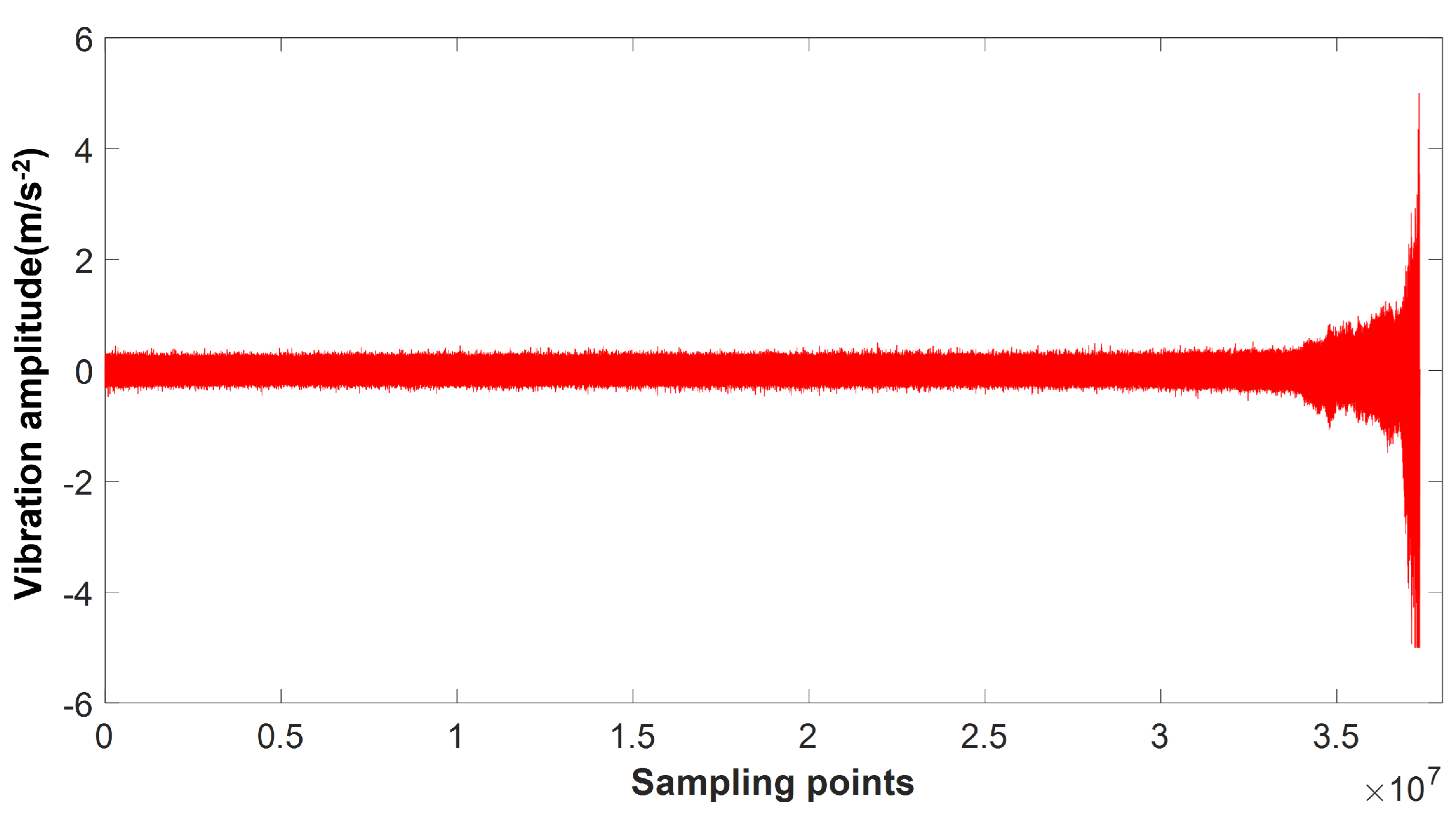
The premise of fault prognosis is to construct health indices that characterize the performance changes in the model based on the data collected by the sensors. Since the characteristic parameters of the vibration signal contain the significant information on model performance changes, in order to construct suitable health indices, it is necessary to extract the characteristic parameters of the model from the original bearing vibration signal. As shown in Table 1, this paper extracts time domain parameters such as the average, variance, root mean square, peak-to-peak value, and kurtosis from time domain signals, and frequency domain parameters such as averages, variances, and root mean squares from frequency domain signals. This paper selects the feature data commonly used in signal processing, but proves that compared with single feature information, the feature information obtained after feature learning of multiple feature information by SAE and EWMA can better reflect the change in bearing health status with time.
The characteristic parameters are the external information of the vibration signal, and different characteristic values reflect the internal information of different aspects of the signal [21]. In order to better construct the model’s health indices, it is necessary to perform feature learning and information fusion on information of all aspects of the vibration signal. Traditional methods for constructing health indices often use machine learning methods such as PCA and LLE to perform component analysis and data dimensionality reduction on feature parameters. In this paper, stacked autoencoders are used to perform feature learning and information mining on model feature parameters. By capturing the inherent information hidden in the feature parameters, the health indices that can characterize the performance changes in the model are constructed. Compared with the traditional health index construction method, the stacked autoencoder has three obvious advantages: (1) The stacked autoencoder is a deep learning model composed of multiple autoencoders. It can rely on the deep structure of the model to autonomously mine information about the model’s characteristic parameters and obtain information about the performance changes in the model hidden under the characteristic parameters. (2) The traditional health index construction method is a machine learning method. Compared with the stacked autoencoder, the feature learning ability and nonlinear data fitting ability are very limited. The stacked autoencoder can perform feature learning and information fusion on feature parameters more comprehensively and accurately, and the constructed health indices can more accurately track the performance changes in the model. (3) The stacked autoencoder model uses self-supervised training, which is very suitable for the construction of model health indices.
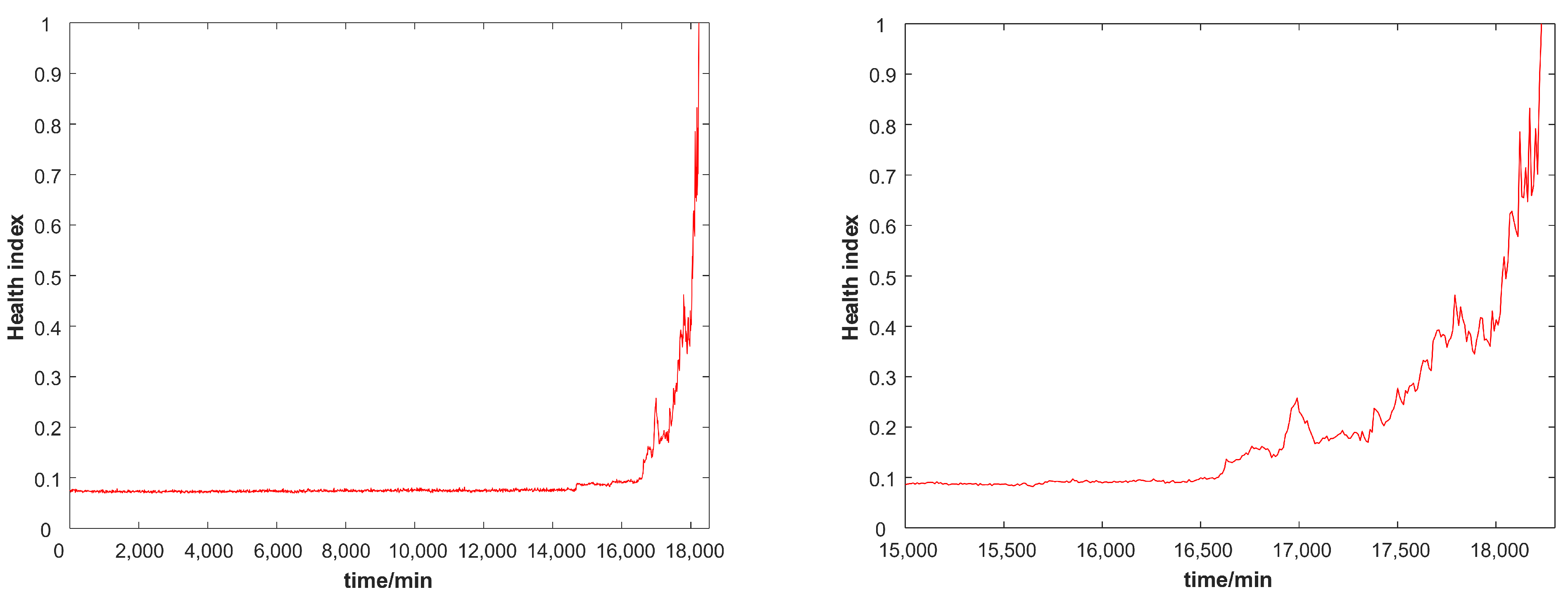
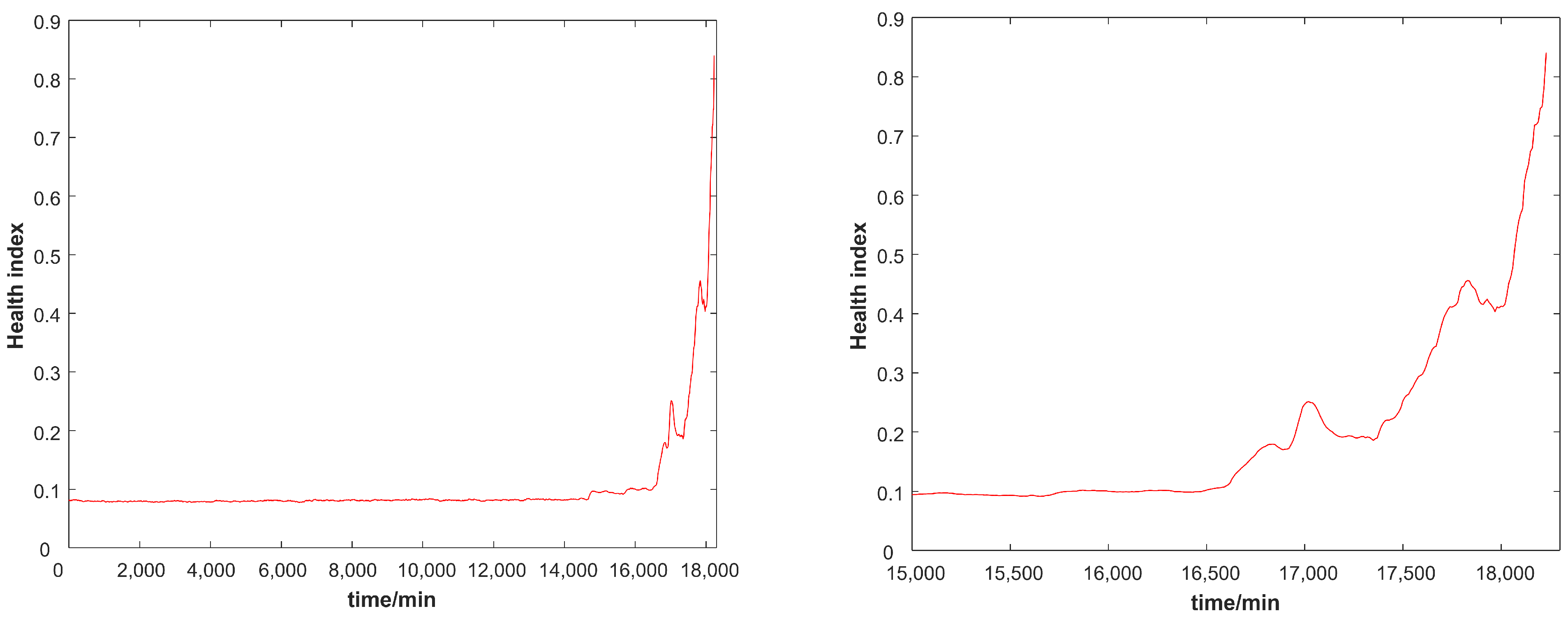
Due to the influence of noise in the vibration signal collected by the sensor, although the constructed health indices can reflect the performance change in the model as a whole, random disturbances appear locally. This not only cannot accurately represent the actual changes in the model, but also directly affects the result of fault prognosis. Therefore, in order to reduce the influence of noise, this paper uses the exponential weighted moving average method to perform further data smoothing of health indices. The exponentially weighted moving average method is a method to determine the estimated value by referring to the current data and historical data simultaneously. The mechanism of the exponential moving average algorithm is described as follows:
f t = α p t + ( 1 α ) f t 1
where f t represents the estimated value; α is a parameter to control the data smoothing effect; p t is the current data; and f t 1 represents the historical data. Equation (7) is a recursive formula. If it is expanded, the mechanism can be described as:
f t = a p t + β p t 1 + β 2 p t 2 + + β t 1 p 1 β = 1 α
The change in configuration should be a continuous change. The exponential weighted moving average method refers to both current data and historical information to evaluate the actual value of the health indices. It can greatly reduce the impact of noise interference and capture mutation information while accurately maintaining the changes in health indices, which is very suitable for the construction of model health indices.

3.2. The Continuous Deep Belief Network

The feature learning effect of health indices directly determines the failure prognosis result. Deep belief networks can quickly and efficiently perform feature learning of health indices by simulating the deep structure of the human brain. Deep belief networks perform feature learning through data discretization, improving the efficiency of feature learning based on sacrificing data continuity. However, the model’s health index is a continuous time series. It is difficult for a standard deep belief network to obtain high-precision fault prognosis results [22]. Through in-depth research on RBMs, Chen et al. proved that RBMs theoretically have the ability to process continuity data, and designed a continuity restricted Boltzmann machine (CRBM) [23]. Based on the research into CRBMs, this paper designs a continuous deep belief network (CDBN) for fault prognosis of health indices.
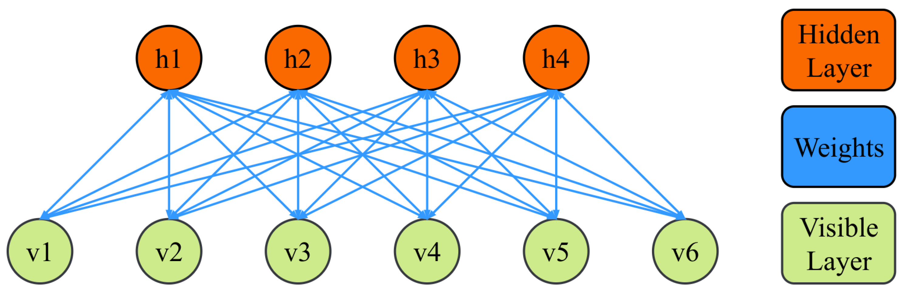
CRBMs are the most basic component and function realization unit of CDBNs, so the CRBM was constructed first. The CRBM is a variant of a standard RBM, created in order to better handle continuous data, so a CRBM model was built on the basis of RBMs. (1) Gaussian noise was added with an average of 0 and a variance of 1 to each unit of the visible layer and the hidden layer to build a continuous random unit. (2) Continuous activation was used to activate the state of each neuron while retaining the sigmoid transfer function, and upper and lower asymptotes were added along with parameters that control the slope of the activation function. (3) The probability discrete binary process was cancelled in a standard RBM. The status of each unit in the CRBM model is as follows:
h j = φ W i j v i + λ N j ( 0 , 1 ) v i = φ W j i h j + λ N i ( 0 , 1 ) φ ( x ) = ϕ L + ϕ H ϕ L × 1 1 + exp ( a x )
where W represents the weight between the visible layer and the hidden layer in the CRBM model; ϕ ( x ) is the activation function of the CRBM; N ( 0 , 1 ) is Gaussian noise with an average of 0 and a variance of 1; λ is a constant; ϕ L and ϕ H are the lower and upper asymptotes, respectively; and α is used to control the slope of the continuity activation function.
The CDBN is a deep learning model made up of multiple CRBMs through the greedy algorithm. The training method of the CDBN is almost the same as the standard DBN, and it also includes two parts: supervised learning and unsupervised learning. The unsupervised learning part is mainly used by each CRBM to train its own model using the MCD algorithm. The greedy algorithm, that is, the hidden layer of the first CRBM, is used as the visible layer of the second CRBM to realize feature learning and information fusion of the input information.
W n + 1 = m W n + η w ( v h v ˜ h ˜ ) a n + 1 = m a n + η a h 2 h ˜ 2 / a n 2
where m is momentum; η is the learning rate; and v ˜ and h ˜ represent the state of the neuron after a Gibbs sample.
The CDBN trains the parameters in the model to a more suitable range through unsupervised learning. During the supervised phase, the CDBN is regarded as an initialized BP neural network as a whole, and the gradient descent method is used for further fine-tuning based on the error of the prediction information and the actual information:
Δ W i j l = η w δ i l s l 1 Δ a i l = η a δ i l z i l / a i l 2
where η is the learning rate; δ i l is the residual of the i-th unit of the model; and z l is the input value of the unit of each layer without passing through the activation function.
The above gradient is the gradient update method for a single sample in the dataset. When the entire dataset is trained, the individual gradients are usually added to obtain the average gradient. After obtaining the gradient value of each parameter, the gradient descent method is used to fine-tune the parameters of the model in the CDBN until the supervised learning is complete.

3.3. The Fault Prognosis Steps Based on the Proposed Method
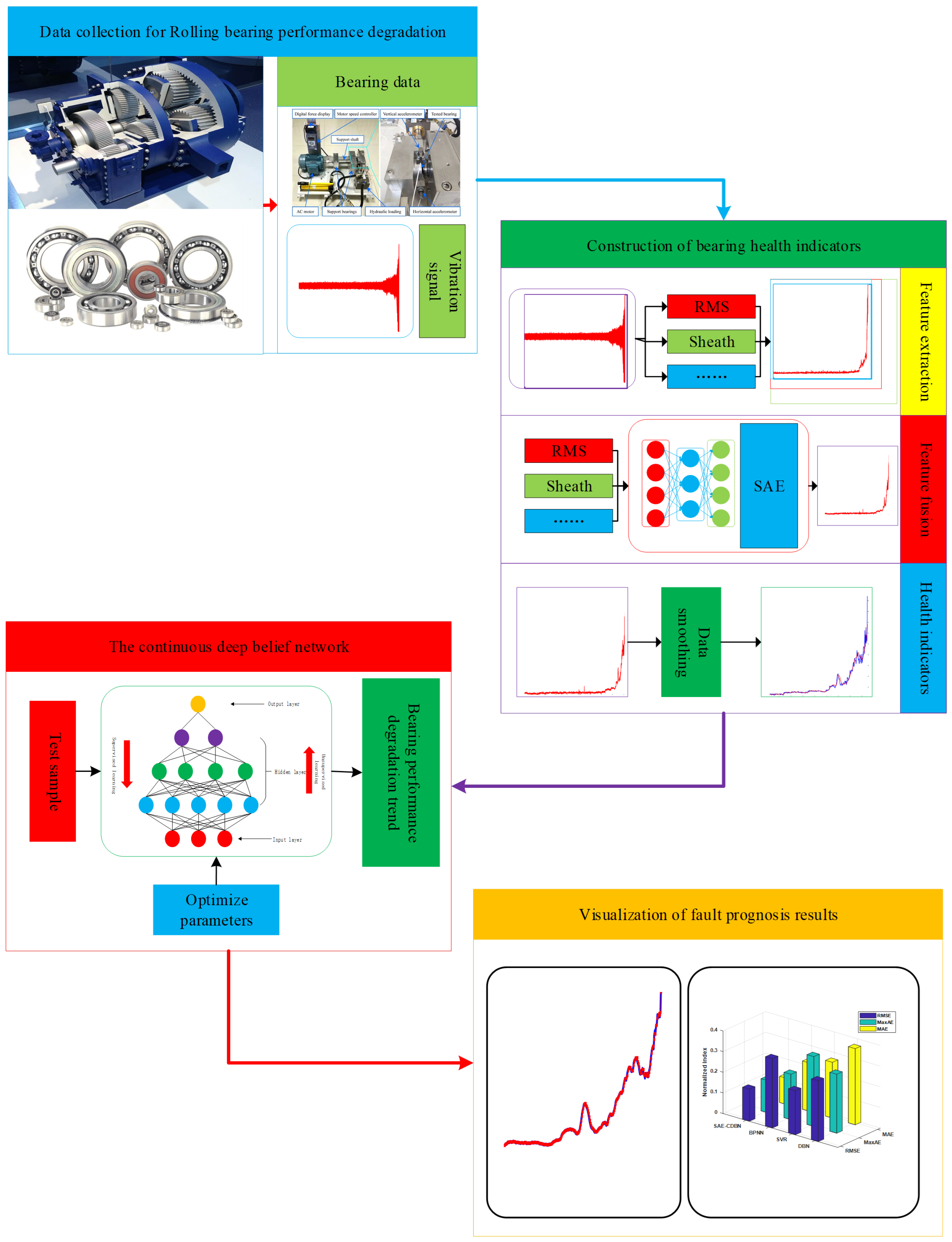
As shown in Figure 4, the intelligent fault prognosis method based on a stacked autoencoder and a continuous deep belief network mainly includes four aspects: data collection, construction of health indices, feature learning of continuous deep belief network, and visualization of fault prediction results.
(1)
Data collection. A bearing performance test experiment is designed and sensors are used to collect bearing lifecycle vibration information.
(2)
Establish health indices. Firstly, feature parameters containing information on bearing performance changes are extracted from the vibration signals collected by the sensors. Then, the stacked autoencoder is used to perform feature learning and information fusion on the extracted feature parameters to construct the health indices that characterize the performance change in the model. Aiming at the local fluctuations in health indices caused by noise, the data are smoothed using the exponentially weighted moving average method to reduce the impact of noise.
(3)
Feature learning for continuous deep belief networks. The model performance change index is a continuous time series. Firstly, a CDBN model suitable for processing continuous data is constructed. Then, its own powerful feature learning ability and information mining ability is used to capture the performance change trends hidden in health indices, and model fault prognosis is performed.
(4)
Visualization of failure results. The fault prognosis results are visualized.

4. Data Processing and Experiment

4.1. The Bearing Data Introduction

In order to verify the effectiveness of the fault prognosis method in this paper, the bearing life cycle data from the University of Cincinnati Intelligent Maintenance System Center are taken as an example to carry out a fault prognosis comparative experiment.
As shown in Figure 5, the bearing accelerated life test bench simulates actual bearing operation: Firstly, an alternating current (AC) motor is used to maintain four Rexnord ZA-2115 double-row bearings mounted on the same connecting rod shaft at a speed of 2000 rpm. A spring mechanism is then used to apply a radial load of 6000 pounds to the bearing. Through two PCB353B33 high-sensitivity quartz integrated circuit piezoelectric (ICP) acceleration sensors mounted on the bearing box, the bearing vibration signal is collected every 10 min at a sampling rate of 20 kHz for one second. During the experiment, an oil circulation system is used to lubricate the bearings and an electromagnetic plug is installed in the oil return pipe to collect debris. When the accumulated debris exceeds a certain level, the test is automatically stopped by an electrical switch. A total of 6324 bearing vibration samples were collected throughout the experiment, and each sample contains 20,480 data points. When the experiment was stopped automatically, the outer ring of bearing No. 3 was checked for faults.
Figure 6 is the full life vibration signal diagram of bearing No. 3 collected by the sensor. When the bearing is in a normal state, the amplitude of the vibration signal is small and the waveform is relatively stable. As the working time increases, the performance of the bearing gradually decreases, and the vibration amplitude gradually increases until it eventually fails completely. Considering that the bearing is in a normal working state for a long time and the performance prediction requirements before model failure in the project, 1824 sets of bearing samples with the model close to fault were selected for the performance evaluation of the method proposed in this paper.

4.2. The Health Indices Construction

The characteristic parameters of the vibration signal means that the information given by model performance changes is explicit. Firstly, the characteristic parameters shown in Table 1 were extracted from the vibration signals collected by the sensors. In this paper, five characteristic parameters, i.e., the average, variance, root mean square, peak-to-peak value, and kurtosis degree, were extracted from the time-domain signal. Three characteristic parameters, i.e., the average, variance, and root mean square, were extracted from the frequency-domain signal. A total of eight feature parameters were extracted from the group samples. As a deep learning network, an autoencoder is used for feature learning and has a self-supervised learning process. By reducing the error without disconnecting between input data and output data, the training of autoencoders is realized. In this paper, eight feature signals extracted from experimental data were put into the autoencoder for feature extraction, and the output results are the results of feature extraction of eight sets of feature data. Different feature parameters contain different model performance information; therefore, in order to comprehensively and accurately learn the performance information hidden in the bearing vibration signal, a stacked autoencoder was used to perform feature learning and information fusion on the extracted feature parameters. Table 2 shows the experimental parameters extracted by the stacked autoencoder used in this paper. The network structure of the stacked autoencoder was 8-15-6-2-1, the activation function was the sigmoid function, the number of iterations was 30, and the noise constant was 0.1. The parameters of the network structure are the results of the experiment, and the parameter information of the autoencoder was determined by continuously adjusting the parameters in Table 2 and comparing the Spilman coefficient of the results.
Figure 7 shows the health indices constructed by the stacked autoencoder by performing feature learning and information fusion on the extracted feature parameters. The abscissa represents the working time of the bearing and the ordinate represents the health index corresponding to the bearing. When the bearing is in a normal healthy state, the health index fluctuates up and down within the range of 0∼0.025. As the working time increases, the performance of the bearing changes gradually, and the health index also changes accordingly. The bearing health index as a whole shows a “rise-down-rise” trend, which is caused by the self-repairing ability of the bearing. As the bearing is in a high-intensity working state for a long time, the performance of the bearing gradually decreases, the bearing fails slightly, and the health index starts to rise. However, continuous work will aggravate the faults in the bearing through wear. The bearing performance improves and the health index reduces. It is worth noting that the self-repairing ability of the bearing is limited, and the performance of the bearing will still decrease with the increase in working time. The process was repeated until the bearing performance completely failed.
Due to the influence of noise on the vibration signal collected by the sensor, as shown in Figure 7, although the health indices constructed by the stacked autoencoder maintain the overall monotonicity, random fluctuations will occur. This will affect the outcome of subsequent fault prognosis. Therefore, this paper uses the exponentially weighted moving average method to further improve the health index. According to experimental experience, the smoothing parameter was set to 1/10, as shown in Figure 8. The noise in our data, which comes from experiments, not only does not accurately represent the change in the actual model, but also directly affects the results of failure prediction. Figure 7 and Figure 8 illustrate the effect of the EWMA. The EWMA refers to both the historical data and the current data, greatly reducing the impact of noise interference and capturing mutation information while accurately maintaining health index trends, which is very suitable for the construction of model health indexes. After the health indices were smoothed by the data, the local disturbance phenomenon was improved, and the influence of noise on the fault prediction was reduced. To more clearly show the details of the health indices construction, the subfigures on the right of Figure 7 and Figure 8 are an expansion of the left subfigures in the range of 15,000∼18,000 min.
The health indices of the model directly affect the results of the subsequent fault prognosis. According to the principle trend in the health indices, as the working time increases, the internal components of the model gradually wear out. In order to verify the effectiveness of the constructed health indices, the health indices that characterize the changes in bearing performance should be related to working hours. There is a non-linear relationship between the health indices and working time. The Spearman coefficient can transform the non-linear relationship between the health indices and working hours into a linear relationship. This paper calculates the Spearman coefficients for different health indicators and times. The calculation of the Spearman coefficient is as follows:
T r e ( X ˜ , T ˜ ) = K k 1 K X ˜ k T ˜ k k 1 K X ˜ k k 1 K T ˜ k K k 1 K X ˜ k 2 k 1 K X ˜ k 2 K k 1 K T ˜ k 2 k 1 K T ˜ k 2
where T ˜ k represents the rank sequence of the k-th time value and X ˜ k represents the rank sequence of the k-th time value corresponding to the health indices.
Table 3 summarizes the Spearman coefficients for the different types of health indices and working hours. By comparing the correlation coefficients of different health indices, the following conclusions can be obtained:
(1)
Compared with a single characteristic parameter model to characterize the performance of the model, the health indices constructed by information fusion of multiple characteristic parameters can more accurately reflect the performance changes of the model.
(2)
Compared with machine learning methods such as PCA and kernel principal component analysis (KPCA), stacked autoencoders as deep learning models can better perform feature learning and information fusion on the extracted feature parameters, and the health indices constructed are more accurate.
(3)
The exponentially weighted moving average can reduce the impact of noise on health indices, and can capture mutation information while maintaining the overall trend of the model. The health indices constructed by combining the advantages of the SAE and the EWMA can better characterize the performance changes in the model and the tendency of the bearing performance to degrade compared to a single characteristic value.

4.3. The Health Indices Fault Prognosis

4.3.1. Data Processing

In order to verify the effectiveness of the proposed fault prognosis method, direct prediction technology was used to process the health indices of the constructed model to characterize the performance changes. According to Taken’s embedding theory, when there is a certain functional relationship between a future value and the first m consecutive value in a single variable time series, the current and historical information can be used to predict the performance change of the future model [24]. This is also true for the real-life engineering problem of predicting the future health indices of bearings. The constructed health indices contain a total of 1825 data points. Based on experimental experience, the regression lag order was set to four, which means that the previous four health indices are used to predict the next moment’s health index. Therefore, 1821 samples were used in the experiment.
Considering that in normal engineering, only the vibration data of the normal working phase of the bearing can be obtained and the complex performance changes at the end of the bearing life, this paper uses the health indices of normal working of the bearing to train the continue deep belief network model, and uses the health indices of the influencing phase to test the model. The envelope spectrum analysis method can demodulate the frequency components in the vibration signal and extract the low frequency fault signal from the high frequency information. Therefore, the envelope spectrum analysis method is used to divide the model’s health indices.
Figure 9 shows the envelope spectrum of the vibration signal collected by the sensor in different periods. When the bearing runs for 14,690 min, although the characteristic information of the bearing outer ring fault is found in the envelope spectrum of the bearing, the amplitude is very small. We believe that the early fault of the bearing has begun, but the impact on the system is small and can be ignored. When the bearing runs for 15,710 min, the amplitude of the fault information is slowly increasing but the increase is still small, so the impact of bearing faults on the system can still be ignored. When the bearing runs for 15,720 min, the amplitude of the fault information in the envelope spectrum of the bearing increases rapidly. Therefore, the impact of the bearing fault on the system cannot be ignored, and the fault is further deepened. When the bearing runs for 18,200 min, the amplitude of the fault information is very large and the bearing outer ring fault is very serious. As shown in Table 4, according to the degree of impact of bearing faults on the system, the bearing health indices are divided into two stages. The first is 0∼15,710 min, where the impact of the bearing fault on the system can be ignored. This stage involves the normal operation of the bearing and the initial state of the fault. In the second stage, from 15,720∼18,250 min, the impact of the bearing failure on the system cannot be ignored. This stage involves accelerated degradation and complete failure of the bearing. The values in Table 4 are derived from Figure 8. When the bearing runs for 15,710 min, the amplitude of the fault message increases slowly, but it is still small, so the impact of bearing failure on the system can still be ignored. When the bearing runs for 15,720 min, the amplitude of the fault message in the bearing envelope spectrum increases rapidly. Therefore, it is believed that the impact of bearing failure on the system cannot be ignored, and the failure is further deepened. Therefore, the data after 15,720 min are selected as the training set and the test set for deep learning. If the data before 15,720 min are used, the learning effect is not obvious due to the small amplitude of the fault characteristics. If the data are used, it means that the corresponding training data are less, which will also affect the results of failure prediction.

4.3.2. The CDBN Parameter Determination Experiment

The CDBN relies on its own deep structure to perform independent feature learning on the bearing’s health indices to achieve fault prognosis of the future bearing’s health indices. The network structure of the CDBN model will directly affect the results of fault prognosis, so on the one hand, too many hidden layers and hidden units will make the model too complex, which causes overfitting and increases the calculation time. On the other hand, too few hidden layers and hidden units can degrade the model performance and affect the fault prognosis results. However, until now, there has been no well-established theory to directly determine the network structure of the model. Therefore, our experimental method was used to determine the suitable network structure of the model by comparing the fault prognosis results of the different CDBN models.
This paper introduces the root mean square error (RMSE), the maximum absolute value error (MaxAE), and the mean absolute value error (MAE) to evaluate the model’s fault prognosis performance. According to the principle of decreasing the number of hidden layer units and repeating experiments to reduce the contingency, a total of 10 fault prognosis experiments with different CBDN structures were performed in this paper. Each group of experiments was repeated five times. The average value of the experimental results was used as the final result.
RMSE = 1 T i = 1 T y i y ˜ i 2
MaxAE = max y i y ˜ i
MAE = 1 T i = 1 T y i y ˜ i
Table 5 summarizes the fault prognosis results of the CDBN models with different network structures. The first three sets of models are the CRBM, the middle four sets of models are the CDBN with two hidden layers, and the last three sets are the CDBN with three hidden layers. Firstly, the training samples in the normal stage were input into each model for autonomous feature learning and information fusion. Then, test samples in the influential stages qwew used for fault prognosis through the trained model. Finally, the appropriate network structure of the CDBN was determined by calculating the RMSE, MaxAE, and MAE of the each model’s fault prognosis results.
The magnitudes of the different evaluation standards were quite different; thus, each index was normalized. Figure 10 shows the fault prognosis results and its trends of CDBN models with different network structures. We can clearly see that under various standards, the CDBN model with the network structure of 4-12-8-1 has the smallest error between the prognosis results and the actual values. The prognosis results of this model are the closest to the future health indices. By comparing the fault prognosis results of the CDBN models with different network structures, the following conclusions can be drawn:
(1)
The feature learning ability and information fusion ability of a single CRBM model are limited. The CDBN model uses the greedy algorithm to combine multiple CRBM models. The feature learning ability and non-linear approximation ability are stronger and the method is more suitable for dealing with complex non-linear prediction problems.
(2)
A model with a more complicated network structure will not have a stronger failure prediction ability. This is because the more complex the network structure, the stronger the ability to learn the features of the model, which may lead to over-learning of the training samples. At the same time as learning the performance of the model, some interference information may be learned, which affects the results of fault prediction.

4.3.3. Fault Prognosis Comparative Experiments

In order to verify the results of the fault prognosis method proposed in the paper, a comparative experiment of this method with traditional fault prognosis methods was carried out using IMS bearing data as an example. The experimental parameters of the CDBN model are shown in Table 6. The structure of the CDBN model was 4-12-8-1. In other words, the input layer of the CDBN model contains 4 units, the first hidden layer contains 12 units, the second hidden layer contains 8 units, and 1 unit in the output layer is used to output the fault prognosis result. The learning rate of the inter-layer weights and the control continuity activation function slope parameter was 0.11, and the noise constant was 0.0001. The upper and lower asymptotes of the continuous activation function were 1 and −1, respectively, and the model was trained 100 times. The experimental parameters of the other traditional intelligent fault prognosis methods are as follows:
(1)
BPNN: The network structure was 4-24-1. The learning rate, momentum, and iteration time were 0.01, 0.9, and 500, respectively.
(2)
SVR: The lag order was four and the penalty parameter and kernel radius were 30 and 0.01, respectively, chosen by 5-fold cross validation. The Gaussian kernel was used.
(3)
DBN: The network structure was 4-12-8-1. The learning rate, momentum, and iteration time were 0.11, 0.9, and 200, respectively.
(4)
LSTM: The network structure was 4-12-8-1. The learning rate, momentum, and iteration time were 0.01, 0.9, and 500, respectively. The network was constructed with a logistic regression layer.
(5)
RNN: The network structure was 4-12-8-1. The learning rate, momentum, and iteration time were 0.37, 0.9, and 700, respectively.
The network was constructed with a sigmoid regression layer.
Figure 11 shows the results of different fault prognosis methods. The ordinate represents the health indices and the abscissa represents the running time of the bearing. The blue line represents the actual health indices of the bearing, while the red line is the future health indices predicted by the model through feature learning of current and historical health indices. Through analysis of the results, it can be found that although the traditional intelligent fault prognosis methods can roughly predict the change in model performance, as the performance change suddenly increases at the end of the model’s life, these methods cannot accurately predict the model’s health indices. However, the fault prognosis method proposed in this paper relies on the strong information fusion ability and continuous data learning ability of the continuous deep belief network, and can still make an accurate fault prognosis at the end of the model’s life.
In order to better evaluate the fault prognosis results of the proposed method, the performance of the fault prognosis method was evaluated from different perspectives using three standards: the RMSE, the MaxAE, and the MAE. The RMSE is mainly used to evaluate the error dispersion of the fault prognosis method, the MaxAE is mainly used to evaluate the individual prognosis ability of the fault prognosis method, and the MAE is mainly used to evaluate the overall prognosis ability of the fault prognosis method. Following the principle of repeating experiments to increase the reliability of experiments, each fault prognosis method was repeated 10 times. The results of the three standards for each method were recorded, and the average and variance were used as the final results. Table 7 shows the results of the fault prognosis method. By comparing the prognosis results of different fault prognosis methods, it can be clearly found that: (1) In the same test sample, the RMSE of the proposed fault prognosis method is the smallest, which means that the dispersion of the prognosis error of this method is the smallest. The model has the best reliability. (2) The proposed fault prognosis method has the smallest MaxAE, which means that the maximum prognosis error of this method is also the smallest among the various methods and the model has the best fault prognosis capability. (3) The MAE of the proposed fault prognosis method is the smallest, which means that the average prognosis error of the method is the smallest and the model’s overall fault prognosis ability is the best. In summary, compared with the traditional intelligent prognosis methods, the fault prognosis method proposed in this paper gives the most accurate prognosis and the highest reliability, regardless of whether it is single or overall.
Figure 12 shows the prognosis results of the fault prognosis methods. The magnitudes of the different standards are quite different; thus, the three indicators were standardized. The X-axis represents the standard for evaluating the fault prognosis method, the Y-axis represents the intelligent fault prognosis method, and the Z-axis represents the standardized evaluation value. It can be clearly seen that the three indicators indicate the fault prognosis method based on the stacked autoencoder and the continuous deep belief network from three perspectives. By learning the current and historical information of the model, the prognosis result is more accurate and close to the actual model value. The proposed fault prognosis method can better predict the performance change in the model. Through comparative experiments, the following conclusions can be drawn:
(1) Compared with shallow learning models such as the BPNN and SVR, the CDBN as a deep learning model can more effectively capture the model’s performance trends with time, and its feature learning ability is stronger and more applicable to information mining and fault prognosis for complex nonlinear data. (2) Compared with the standard DBN model, the CDBN has improved feature learning and information mining abilities on continuous time series through the improvement of the model, and solves the problem of the standard DBN model not having a high accuracy for continuous data fault prognosis. (3) Compared with RNN and LSTM models, the CDBN has an improved feature learning ability and gives more reliable fault prognoses.

5. Conclusions

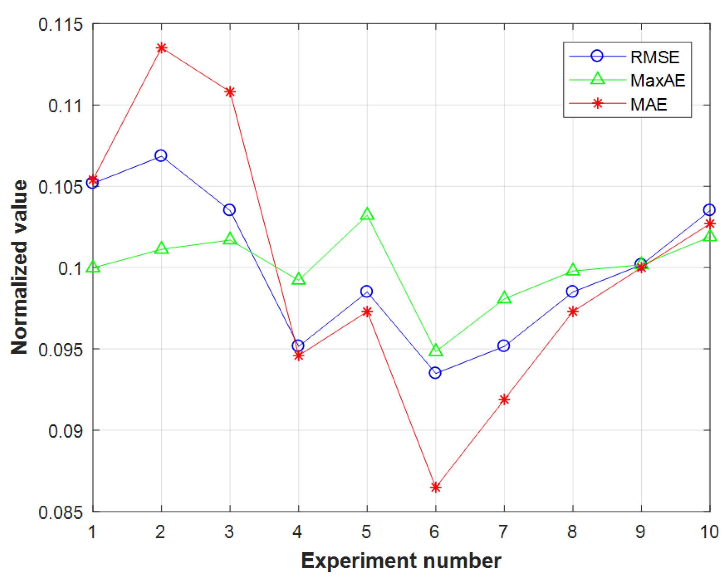
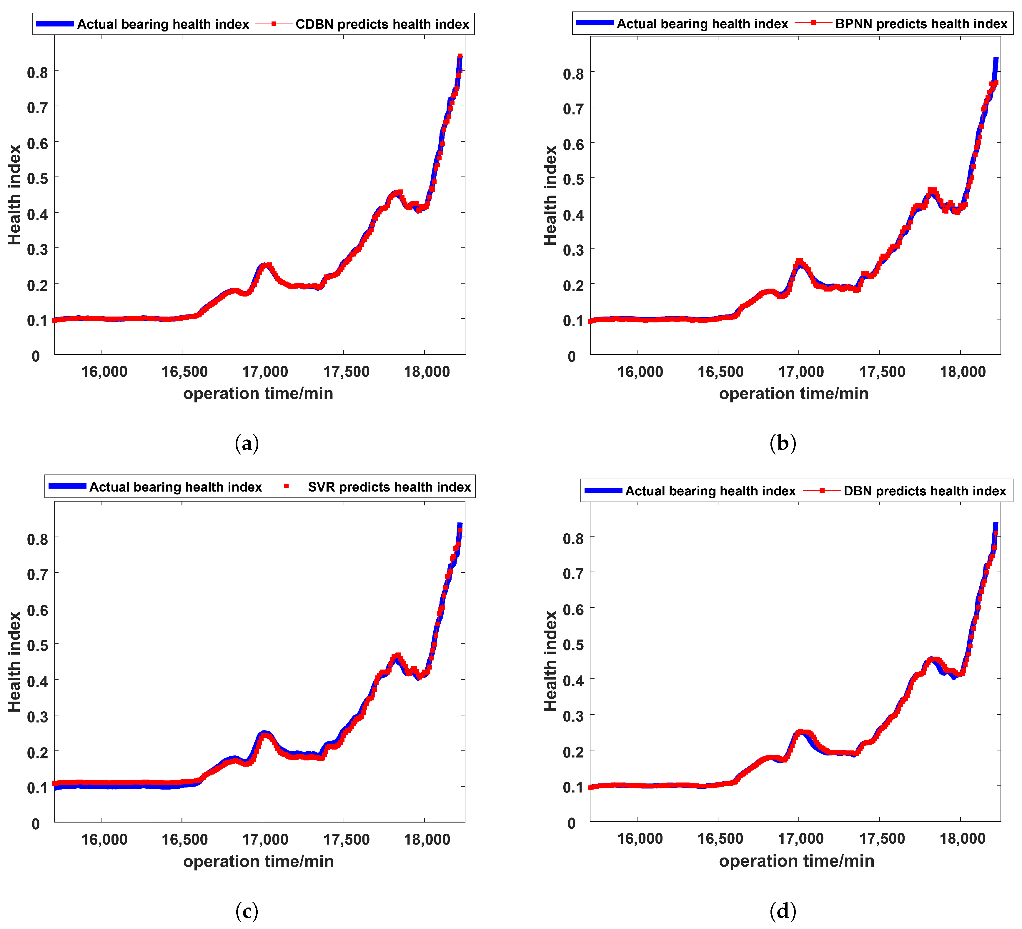
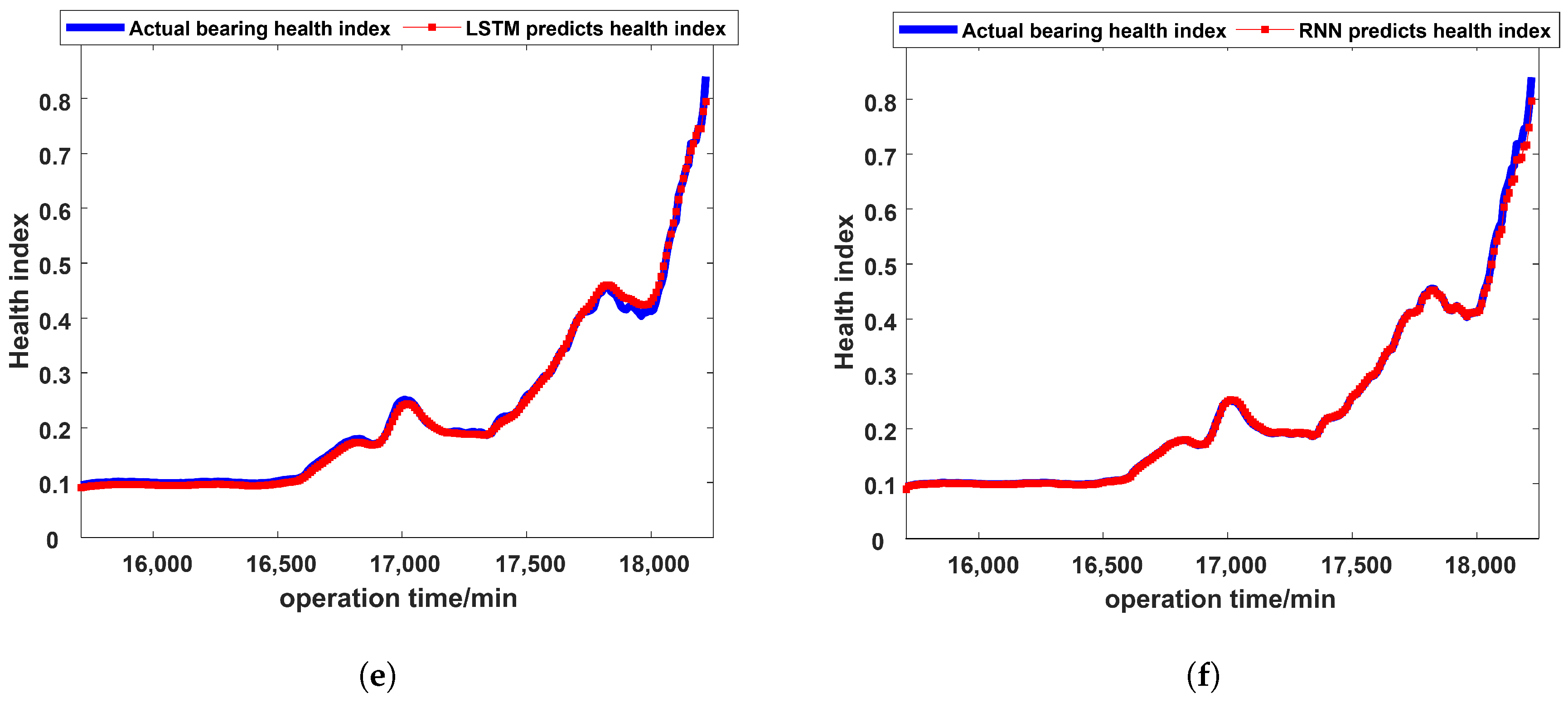
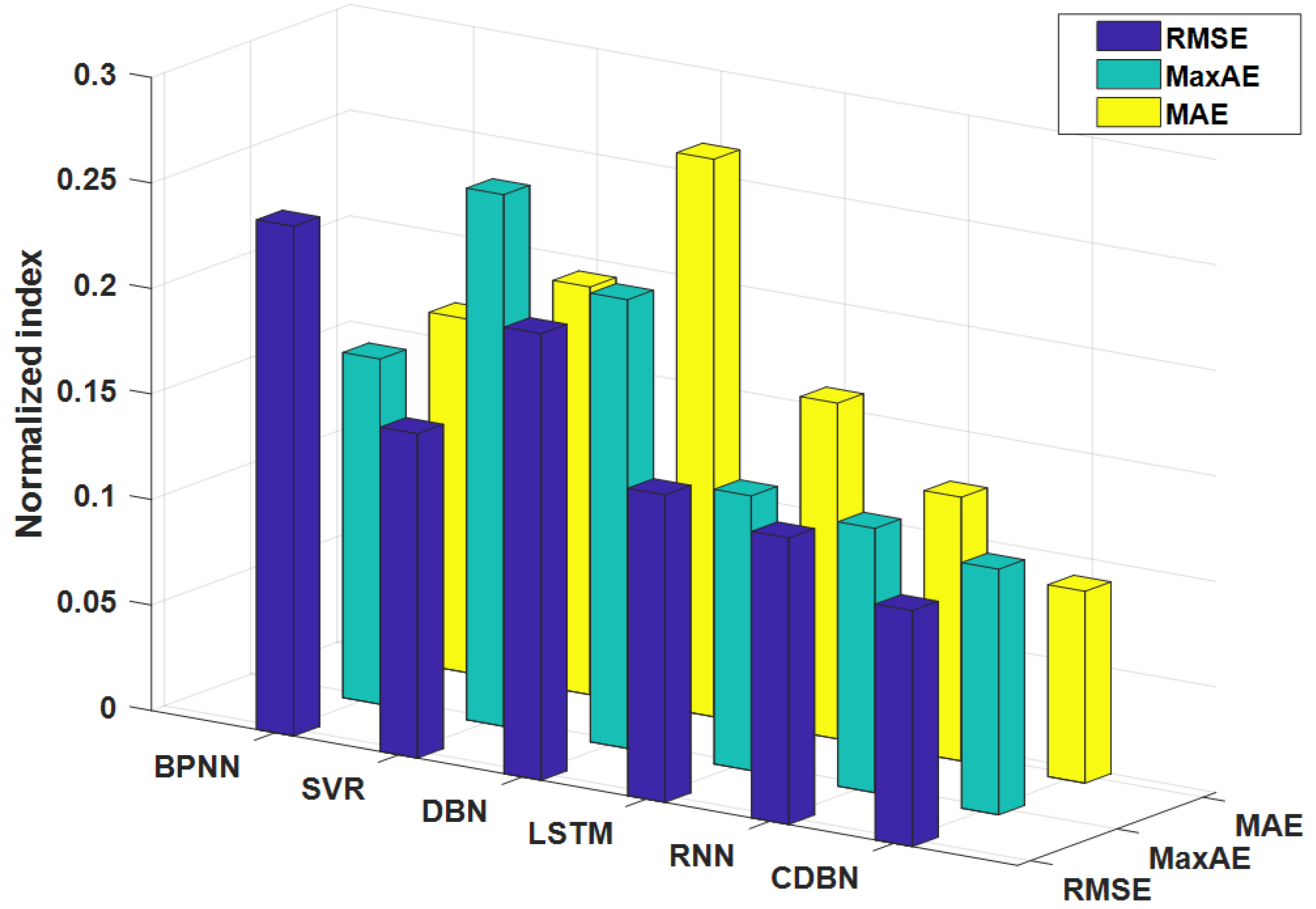
This paper is based on two aspects: the construction of health indices that characterize model performance changes and the fault prognosis of health indices. Combining the strong feature learning capabilities of stacked autoencoders and the continuous information fusion capabilities of continuous deep belief networks, a novel intelligent fault prognosis method based on a stacked autoencoder and a continuous deep belief network is proposed. This method consists of two parts: (1) The stacked autoencoder is used to perform feature learning and information fusion on the extracted feature parameters to build the health indices that characterize the performance change in the model. To solve the problem of local random fluctuations in health indices caused by noise, the exponential weighted moving average method is used to smooth the data, which greatly reduces the impact of noise on health indices. By comparing the performance of different health indices with the performance of actual models, it is proven that the proposed method can more accurately represent the changes in model performance. (2) Continuous deep belief networks are used to perform feature learning and fault prognosis on health indices. In order to verify the fault prognosis ability of the CDBN, a comparative experiment of intelligent prognosis methods was performed. The method in this paper evaluates the performance of the BPNN, SVR, DBN, LSTM, RNN, and the proposed method, CDBN. Furthermore, the normalized RMSE, MaxAE, and MAE indices are as low as 5.6 × 10 3 , 4.98 × 10 2 , and 3.2 × 10 3 , respectively. The experimental results prove that compared with traditional intelligent prognosis methods, the CDBN model used in this paper has stronger feature learning capabilities, can determine the regularity of model performance changes in health indices, and can accurately predict changes in bearing performance.

Author Contributions

Conceptualization, Y.Z. (Yibin Zhang); methodology, Y.Z. (Yibin Zhang); software, Y.Z. (Yibin Zhang); validation, Y.Z. (Yibin Zhang); formal analysis, C.Z. (Chao Zhang) and Y.Z. (Yong Zhou); investigation, Q.H.; data curation, Y.Z. (Yibin Zhang); writing—-original draft preparation, Y.Z. (Yibin Zhang); writing—-review and editing, Q.H.; visualization, Y.Z. (Yibin Zhang); supervision, C.Z. (Chao Zhang) and Y.Z. (Yong Zhou); project administration, C.Z. (Chao Zhang); funding acquisition, C.Z. (Chao Zhang). All authors have read and agreed to the published version of the manuscript.

Funding

This research was funded by the the National Research Projects of China (JCKY2021608B018, JSZL202160113001, and JSZL2022607B002-081).

Data Availability Statement

Conflicts of Interest

The authors declare no conflict of interest.

Abbreviations

The following abbreviations are used in this manuscript:
SAEStacked autoencoder
EWMAExponentially weighted moving average
PCAPrincipal component analysis
LLELocally linear embedding
IMSIntelligent maintenance systems
DBNDeep belief network
RBMRestricted Boltzmann machine
BPBack propagation
DBNDeep belief network
MCDMinimizing contrastive divergence
CRBMContinuity restricted Boltzmann machine
CDBNContinuous deep belief network
KPCAKernel principal component analysis
RMSERoot mean square error
MaxAEMaximum absolute value error
MAEMean absolute value error
SVRSupport vector regression
LSTMLong short-term memory
RNNRecurrent neural network

References

  1. Tian, F.; Luo, R.; Jia, L. Non-Stationary Feature Extraction Method for Mechanical Faults and Its Application; National Defense Industry Press: Beijing, China, 2014. [Google Scholar]
  2. Peng, Y.; Dong, M. A prognosis method using age-dependent hidden semi-Markov model for equipment health prediction. Mech. Syst. Signal Process. 2011, 25, 237–252. [Google Scholar] [CrossRef]
  3. Yu, M.; Xiao, C.; Wang, H.; Jiang, W.; Zhu, R. Adaptive Cuckoo Search-Extreme Learning Machine Based Prognosis for Electric Scooter System under Intermittent Fault. Actuators 2021, 10, 283. [Google Scholar] [CrossRef]
  4. Yu, M.; Lu, H.; Wang, H.; Xiao, C.; Lan, D.; Chen, J. Computational intelligence-based prognosis for hybrid mechatronic system using improved wiener process. Actuators 2021, 10, 213. [Google Scholar] [CrossRef]
  5. Janjarasjitt, S.; Ocak, H.; Loparo, K. Bearing condition diagnosis and prognosis using applied nonlinear dynamical analysis of machine vibration signal. J. Sound Vib. 2008, 317, 112–126. [Google Scholar] [CrossRef]
  6. Lei, Y.; Liu, Z.; Lin, J.; Lu, F. Phenomenological models of vibration signals for condition monitoring and fault diagnosis of epicyclic gearboxes. J. Sound Vib. 2016, 369, 266–281. [Google Scholar] [CrossRef]
  7. Huang, D.; Huang, X.; Fan, M.; Xiong, Z. Mixed fault prediction based on Kalman filtering and expert system. Comput. Simul. 2005, 22, 150–152. [Google Scholar]
  8. Du, Z.; Li, X.; Zheng, Z.; Mao, Q. Fault prediction with combination of strong tracking square-root cubature Kalman filter and autoregressive model. Control Theory Appl. 2014, 31, 1047–1052. [Google Scholar]
  9. Lin, P.; Wang, K. Particle Filter Fault Prediction Based on Fuzzy Closeness Degree. Appl. Comput. Syst. 2017, 26, 134–138. [Google Scholar]
  10. Baptista, M.; de Medeiros, I.P.; Malere, J.P.; Nascimento, C.; Prendinger, H.; Henriques, E.M. Comparative case study of life usage and data-driven prognostics techniques using aircraft fault messages. Comput. Ind. 2017, 86, 1–14. [Google Scholar] [CrossRef]
  11. Civera, M.; Surace, C. Non-destructive techniques for the condition and structural health monitoring of wind turbines: A literature review of the last 20 years. Sensors 2022, 22, 1627. [Google Scholar] [CrossRef]
  12. Zhang, P.; Zhou, L.; Zhang, Z.; Li, J. Analysis and Prediction of Transformer Overheating Fault Based on Chaotic Characteristics of Oil Chromatogram. High Volt. Appar. 2019, 55, 237–243. [Google Scholar]
  13. Peng, G.; Zhou, Z.; Tang, S.; Wu, T.; Wu, X. Transformer Fault Prediction Based on Timing Analysis and Variable Correction. Electron. Meas. Technol. 2018, 41, 96–99. [Google Scholar]
  14. Yan, J.; Koç, M.; Lee, J. A prognostic algorithm for machine performance assessment and its application. Prod. Plan. Control 2004, 15, 796–801. [Google Scholar] [CrossRef]
  15. Rigamonti, M.G.; Baraldi, P.; Zio, E.; Roychoudhury, I.; Goebel, K.; Poll, S. Ensemble of optimized echo state networks for remaining useful life prediction. Neurocomputing 2017, 281, 121–138. [Google Scholar] [CrossRef] [Green Version]
  16. Xu, J.; Liu, L.; Zhang, L.; Duan, W.; Liu, S. Research on multi-label prediction model of shield fault based on PCA-LSTM. J. Shandong Agric. Univ. (Nat. Sci. Ed.) 2019, 50, 1005–1009. [Google Scholar]
  17. Li, X.; Jiang, H.; Xiong, X.; Shao, H. Rolling bearing health prognosis using a modified health index based hierarchical gated recurrent unit network. Mech. Mach. Theory 2019, 133, 229–249. [Google Scholar] [CrossRef]
  18. Civera, M.; Surace, C. An application of instantaneous spectral entropy for the condition monitoring of wind turbines. Appl. Sci. 2022, 12, 1059. [Google Scholar] [CrossRef]
  19. Zhou, F.; Gao, Y.; Wang, J.; Wen, C. Early diagnosis and life prognosis for slowly varying fault based on deep learning. J. Shandong Univ. (Eng. Sci. Ed.) 2017, 47, 30–37. [Google Scholar]
  20. Hinton, G.E.; Osindero, S.; Teh, Y.W. A Fast Learning Algorithm for Deep Belief Nets. Neural Comput. 2006, 18, 1527–1554. [Google Scholar] [CrossRef]
  21. Schmidhuber, J. Deep learning in neural networks: An overview. Neural Netw. 2015, 61, 85–117. [Google Scholar] [CrossRef] [Green Version]
  22. Guo, L.; Li, N.; Jia, F.; Lei, Y.; Lin, J. A recurrent neural network based health indicator for remaining useful life prediction of bearings. Neurocomputing 2017, 240, 98–109. [Google Scholar] [CrossRef]
  23. Chen, H.; Murray, A.F. Continuous restricted Boltzmann machine with an implementable training algorithm. IEE Proc.-Vis. Image Signal Process. 2003, 150, 153–158. [Google Scholar] [CrossRef] [Green Version]
  24. Takens, F. Detecting Strange Attractors in Turbulence. In Dynamical Systems and Turbulence, Warwick 1980; Springer: Berlin/Heidelberg, Germany, 1981. [Google Scholar]
Figure 1. The structure of an autoencoder.
Actuators 12 00117 g001
Figure 2. The structure of a stacked autoencoder.
Actuators 12 00117 g002
Figure 3. The structure of the restricted Boltzmann machine.
Actuators 12 00117 g003
Figure 4. Bearing fault prognosis steps based on the proposed method.
Actuators 12 00117 g004
Figure 5. The bearing accelerated life test bench.
Actuators 12 00117 g005
Figure 6. Variation in vibration signal over the full life of a rolling bearing.
Actuators 12 00117 g006
Figure 7. The health indices constructed by the SAE, where the right subgraph is a zoomed graph of the left subfigure in the range of 15,000∼18,000 min.
Actuators 12 00117 g007
Figure 8. The health indices constructed by the EWMA and the SAE, where the right subgraph is a zoomed graph of the left subfigure in the range of 15,000∼18,000 min.
Actuators 12 00117 g008
Figure 9. The envelope spectrum of the vibration signal collected by the sensor during different periods. (a) Envelope spectrum for a bearing running at 14,690 min. (b) Envelope spectrum for a bearing running at 15,710 min. (c) Envelope spectrum for a bearing running at 15,720 min. (d) Envelope spectrum for a bearing running at 18,200 min.
Actuators 12 00117 g009
Figure 10. The fault prognosis results of CDBN models with different network structures.
Actuators 12 00117 g010
Figure 11. The results of different fault prognosis methods. (a) The fault prognosis results of the CDBN. (b) The fault prognosis results of the BPNN. (c) The fault prognosis results of the SVR. (d) The fault prognosis results of the DBN. (e) The fault prognosis results of the LSTM. (f) The fault prognosis results of the RNN.
Actuators 12 00117 g011aActuators 12 00117 g011b
Figure 12. Performance evaluation chart of different fault prognosis methods.
Actuators 12 00117 g012
Table 1. Signal characteristic value formula.
Signal CharacteristicCalculation Formula
Root mean square X ms = 1 N i = 1 N X i 2
Average value X ms = 1 N i = 1 N X i
Variance X var = 1 N i = 1 N X i X mean 2
Kurtosis K = 1 N i = 1 N X i μ σ 4
Peak-to-peak value X p p = X m a x X m i n
Table 2. Experimental parameters of the stacked autoencoder.
Parameters
Network structure8-15-6-2-1
Activation functionSigmoid function
The number of iterations30
The noise constant0.1
Table 3. Correlation between characteristic indicators and time.
Vibration SignalEigenvaluesSpearman Coefficient
Health indexSAE+EWMA0.8738
SAE0.7527
PCA0.7404
KPCA0.7402
Time domainAveragee0.7101
Variance0.7259
RMS0.7246
Peak-to-peak0.5911
Kurtosis0.6381
Frequency domainAverage0.7042
Variance0.5784
RMS0.7238
Table 4. The division of health indices.
Operating HoursHealth Indices Stage
0∼15,710 minThe bearing fault has a negligible effect on the system
15,720∼18,250 minThe bearing fault has a considerable effect on the system
Table 5. Influence of different CDBN network structures on bearing fault prognosis.
NumberCDBN Network StructureRMSE ( 10 3 )MaxAE ( 10 2 )MAE ( 10 3 )
14-8-16.3 ± 0.345.25 ± 0.1423.9 ± 0.23
24-12-16.4 ± 0.425.31 ± 0.1364.2 ± 0.26
34-16-16.2 ± 0.255.34 ± 0.1534.1 ± 0.24
44-16-12-15.7 ± 0.435.21 ± 0.1233.5 ± 0.31
54-16-8-15.9 ± 0.325.42 ± 0.1423.6 ± 0.24
64-12-8-15.6 ± 0.414.98 ± 0.1353.2 ± 0.19
74-12-4-15.7 ± 0.525.15 ± 0.1383.4 ± 0.32
84-12-8-4-15.9 ± 0.515.24 ± 0.1413.6 ± 0.36
94-16-8-4-16.0 ± 0.325.26 ± 0.1563.7 ± 0.25
104-16-12-4-16.2 ± 0.435.35 ± 0.1483.8 ± 0.43
Table 6. Experimental parameters of the continuous deep belief network.
Parameters
Network structure4-12-8-1
Learning rate0.11
Iteration times100
Noise constant0.0001
Lower and upper asymptotes−1, 1
Table 7. Performance evaluation under four methods.
NetworkRMSE ( 10 3 )MaxAE ( 10 2 )MAE ( 10 3 )
CDBN5.6 ± 0.414.98 ± 0.143.2 ± 0.19
BPNN12.1 ± 0.157 ± 0.525.9 ± 0.55
SVR7.710.786.8
DBN10.6 ± 0.729.1 ± 0.749.3 ± 0.5
LSTM7.3 ± 0.315.57 ± 0.255.6 ± 0.35
RNN6.8 ± 0.425.36 ± 0.224.4 ± 0.34
Disclaimer/Publisher’s Note: The statements, opinions and data contained in all publications are solely those of the individual author(s) and contributor(s) and not of MDPI and/or the editor(s). MDPI and/or the editor(s) disclaim responsibility for any injury to people or property resulting from any ideas, methods, instructions or products referred to in the content.

