Robust Liquid Level Control of Quadruple Tank System: A Nonlinear Model-Free Approach

Abstract

In this paper, two new versions of modified active disturbance rejection control (MADRC) are proposed to stabilize a nonlinear quadruple tank system and control the water levels of the lower two tanks in the presence of exogenous disturbances, parameter uncertainties, and parallel varying input set-points. The first proposed scheme is configured from the combination of a modified tracking differentiator (TD), modified super twisting sliding mode (STC-SM), and modified nonlinear extended state observer (NLESO), while the second proposed scheme is obtained by aggregating another modified TD, a modified nonlinear state error feedback (MNLSEF), and a fal-function-based ESO. The MADRC schemes with a nonlinear quadruple tank system are investigated by running simulations in the MATLAB/SIMULINK environment and several comparison experiments are conducted to validate the effectiveness of the proposed control schemes. Furthermore, the genetic algorithm (GA) is used as a tuning algorithm to parametrize the proposed MADRC schemes with the integral time absolute error (ITAE), integral square of the control signal (ISU), and integral absolute of the control signal (IAU) as an output performance index (OPI). Finally, the simulation results show the robustness of the proposed schemes with a noticeable reduction in the OPI.

1. Introduction

Industrial processes are physical systems that comprise a group of operations to complete a specific requirement. Interaction during the industrial process is essential to most industrial processes; this interaction may cause multiple variables which increase the complexity of nonlinear systems. 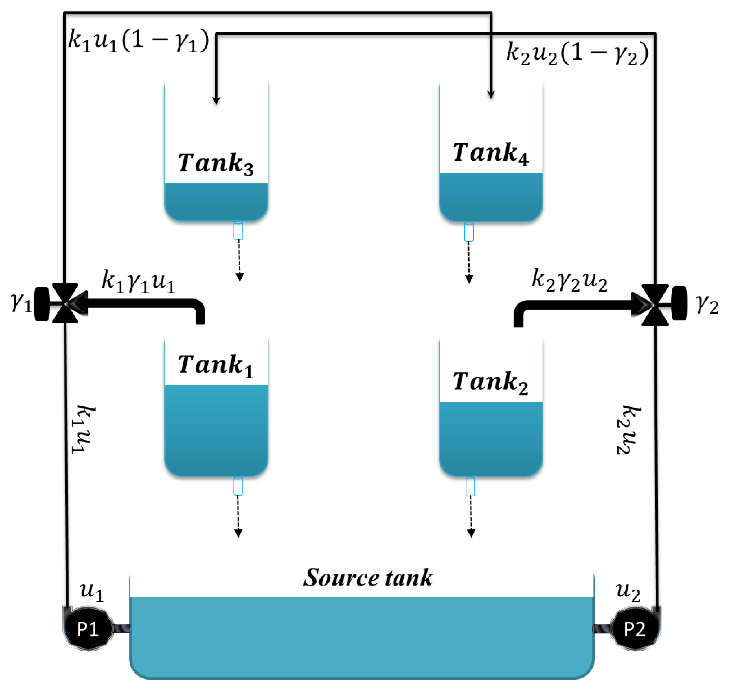One of these industrial processes is the chemical industry, which has become significant to other industries in the last century such as the transport and pharmaceutical industries, in turn contributing to the development of the economy [1]. The four-tank system is an example of the industrial chemical process proposed by [1] at the end of 1995. It is considered one of the multivariable systems with strong nonlinearity and is used as a laboratory process for understanding the control concept for the multivariable control system [1,2].

At present, several control strategies have been proposed to study and control the performance of the four-tank system, from conventional simple methods to more accurate and complex methods. The author of [3] presented four controllers: the linear quadratic regulator (LQR), linear quadratic Gaussian regulator (LQGR), $H_2$ controller, and $H_{\infty }$ controller. Simulation results showed the effectiveness of the LQR in providing a good percentage with regard to settling time. However, it showed a noticeable overshoot in the output response. Recently, some researchers considered the problem of disturbance and delay in the four-tank system and studied the performance of the system under these conditions. Authors in [4] developed a decentralized nonlinear robust model predictive control (MPC). A comparison between the decentralized MPC, a centralized MPC, and a cascaded PI controller was conducted. Moreover, the author of [5] proposed a second-order sliding mode controller, which is a twisting algorithm (TA) based controller. A comparison between the TA and a conventional sliding mode controller (SMC) was undertaken, and the simulation results showed that the TA performed better than the SMC in chattering reduction and disturbance rejection. In addition, the author of [6] designed and implemented two controllers: the adaptive pole placement controller (APPC) and robust adaptive sliding mode controller (ASMC). A comparison between the APPC, ASMC, and the conventional PID was conducted under different conditions such as with reference tracking, exogenous disturbance applied to the four-tank system, and parameter uncertainties. The results showed that the ASMC has better transient and disturbance attenuation and a faster response than both APPC and PID. Furthermore, the author of [7] presented a developed version of the four-tank system with SMC-based feedback linearization to stabilize the system within a specific range. The time-delayed four-tank system has been controlled using various techniques, such as SMC, $H_{\infty }$ observer-based robust control, fuzzy control, and neural control [8,9,10,11,12], while some authors have used the disturbance rejection technique as in [13], wherein the author presented the design of a nonlinear disturbance observer-based port-controlled Hamiltonian (PCH) with a basic feedback controller. Simulation results showed that the proposed method had a better response and was more robust to the disturbance than the terminal sliding mode control. A nonlinear disturbance observer has been introduced to estimate disturbance along with a novel input/output feedback linearization controller. In [14], a comparison between this proposed method, PID, and a disturbance observer-based sliding mode controller (DOBSMC) was conducted and showed that the proposed method improves the robustness of the system against disturbance and has superior performance compared with both PID and DOBSMC. The authors in [15] studied a sliding mode observer (SMO) to estimate the valve ratios and higher-order sliding mode controller (HOSM) to ensure accurate performance and to attenuate chattering. The simulation results of the sliding mode observer based on the higher-order sliding mode controller showed that the proposed method was stable and accurately estimated the unknown parameter. Moreover, a comparison between the super twisting controller (STA) and the conventional sliding mode controller has been conducted and showed the robustness and the smoothing feature of the STA. In addition, the authors in [16] proposed a new linear active disturbance rejection control (LADRC) with a nonlinear function. A comparison between the PID, LADRC, and ADRC was conducted. The simulation results showed that the proposed LADRC provides good steady-state performance, fast-tracking, and eliminates disturbance more accurately than PID and conventional LADRC. Finally, in [17], the authors proposed two disturbance rejection control laws which were designed and tuned using Embedded Model Control to solve two problems, the first being the regulation of the water levels of the lower tanks, and the second being the regulation of the water levels of the four tanks. Although all the above studies proposed excellent and accurate controllers for the four-tank system, there are still some drawbacks in their work. Some of the above studies used a linearized model of the four-tank system [1,2]. As a result, these controllers were incapable of following the nonlinear dynamics of the system, especially in practical implementation. Moreover, the controllers could not handle the nonlinearity or cancel the effect of the applied disturbance in a sufficient way. Thus, the main goal of this research is to design robust control laws with the nonlinear four-tank system and in consideration of the problems of disturbance, uncertainty, and reference tracking.

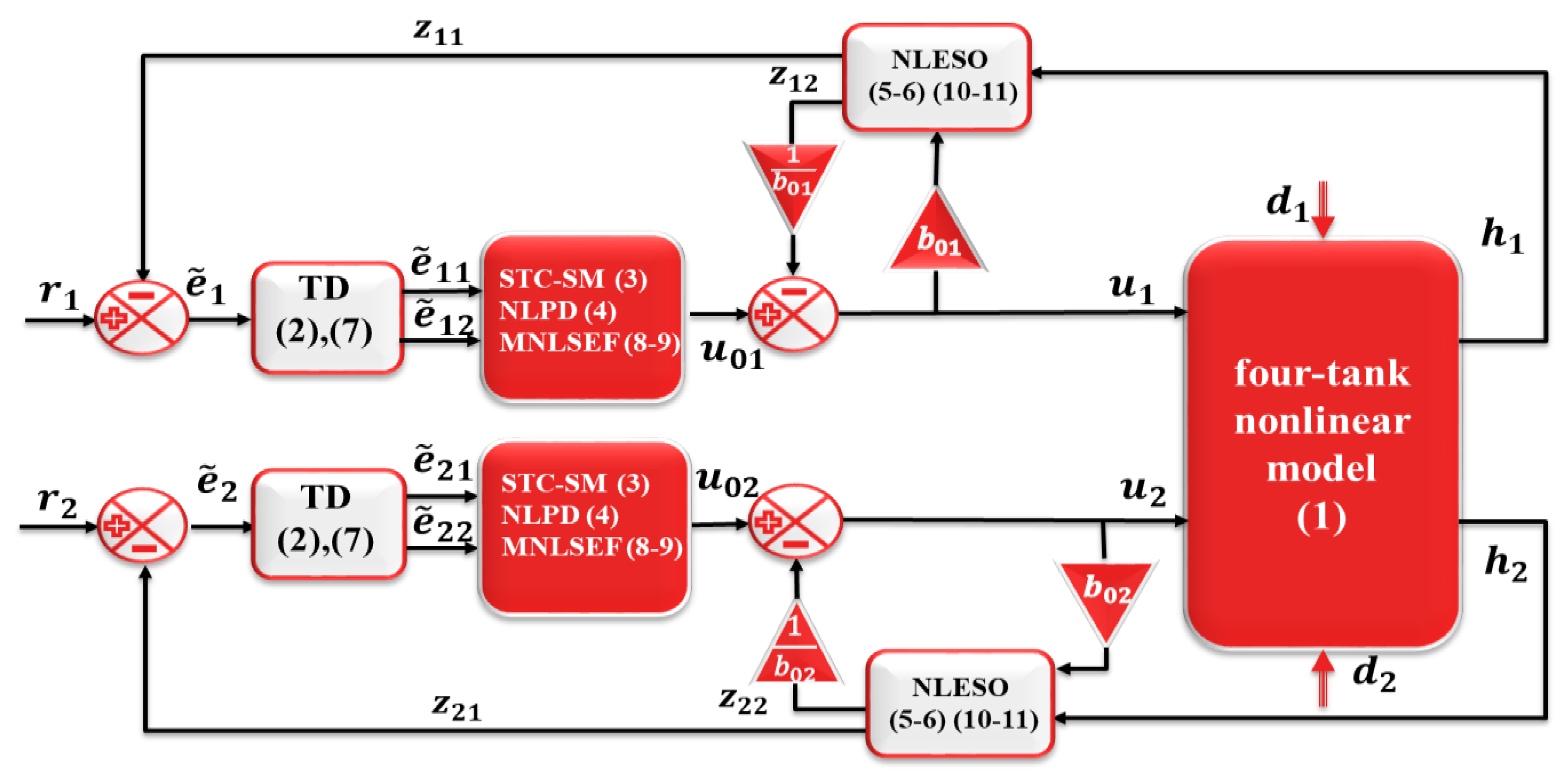
Motivated by the aforementioned studies, two schemes of modified active disturbance rejection control (MADRC) are proposed with the nonlinear model of the four-tank system. The modification part of the MADRC is presented as follows:

i.

The proposed tracking differentiator is used in the control unit to provide the error signal and its derivative.

ii.

The proposed super twisting sliding mode controller (STC-SM), nonlinear proportional derivative (NLPD), and modified nonlinear state error feedback (MNLSEF) are used as nonlinear state error feedback (NLSEF) instead of the conventional NLSEF proposed by [18].

iii.

The modified nonlinear extended state observer (MNLESO) and fal function ESO are used instead of the linear extended state observer (LESO) [19].

The advantages of our proposal are that it may overcome problems presented previously such as nonlinearity, strong interacting, disturbance, uncertainty of the parameters and that it is able to track any applied reference.

To the best of our knowledge, a super twisting controller with improved active disturbance rejection control has not yet been proposed in the literature. This model solves the problem of the four-tank system in a significant and accurate way, which is our incentive for continuing this research endeavor.

The rest of this paper is organized as follows: Section 2 presents the problem statement. The modeling of the four-tank system is presented in Section 3, and the design of the modified ADRC is introduced in Section 4. The convergence of the proposed control schemes is then demonstrated in Section 5. Section 6 demonstrates the simulation results and provides a discussion. Finally, the conclusions of this paper are given in Section 7.

2. Problem Statement

Suppose the nonlinear model of the four-tank system under the presence of the disturbance can be written as

$$\left\{\begin{array}{l}\dot{x}=𝒻\left(x_1,\cdots ,x_4\right)+g\left(x\right)u+d\left(t\right)\\ y=x\end{array}\right.$$

(1)

where $\stackrel{\rightharpoonup }{x}\in {ℝ}^4,$ $\stackrel{\rightharpoonup }{x}=\left[\begin{array}{c}{x}_1\\ x_2\\ x_3\\ x_4\end{array}\right], \stackrel{\rightharpoonup }{x}={\left[x_1 x_2 x_3 x_4\right]}^T$ is the water level in the first, second, third, and fourth tank, respectively, $\stackrel{\rightharpoonup }{y}\in {ℝ}^2,y=\left[x_1,x_2\right]$ are the measured output, and $\stackrel{\rightharpoonup }{u}\in {ℝ}^2,\stackrel{\rightharpoonup }{u}=\left[u_1,u_2\right]$ are the control input required to be designed to stabilize and track the desired setpoint value of the water level of the two lower tanks and to eliminate the effect of the unknown exogenous disturbance $d\left(t\right)$ and system parameter uncertainty applied to the four-tank system.

3. Mathematical Modeling of Nonlinear Four-Tank System

As can be seen from Figure 1, the four-tank system consists of two water pumps, two two-way valves, a source tank, and four tanks. The water pump₁ (M₁) draws water from the source tank and distributes it to tank₁ and tank₄ via valve₁. Similarly, the water pump₂ (M₂) draws water from the source tank and distributes it to tank₂ and tank₃ via valve₂. It is important to note the amount of water delivered to the tanks depends on the valve constant (i.e., ${\gamma }_1$ and ${\gamma }_{2 }$). The nonlinear mathematical model of the four-tank system is given in [1]:

$$\left\{\begin{array}{l}{\dot{h}}_1= - \frac{{\mathrm{a}}_1}{A_1}\sqrt{2g{h}_1}+\frac{{\mathrm{a}}_3}{A_1}\sqrt{2g{h}_3}+\frac{{\gamma }_{1 }{k}_{F{T}_1}}{A_1} \left(u_1+d_1\right)\\ {\dot{h}}_2= - \frac{{\mathrm{a}}_2}{A_2}\sqrt{2g{h}_2}+\frac{{\mathrm{a}}_4}{A_2}\sqrt{2g{h}_4}+\frac{{\gamma }_{2 }{k}_{F{T}_2}}{A_2} \left(u_2+d_2\right)\\ {\dot{h}}_3= - \frac{{\mathrm{a}}_3}{A_3}\sqrt{2g{h}_3}+\frac{\left(1 - {\gamma }_2 \right)k_{F{T}_2}}{A_3} u_2\\ {\dot{h}}_4= - \frac{{\mathrm{a}}_4}{A_4}\sqrt{2g{h}_4}+\frac{\left(1 - {\gamma }_1 \right)k_{F{T}_1}}{A_4} u_1\\ y_1=k_c{h}_1\\ y_2=k_c{h}_2\end{array}\right.$$

(2)

where $A_i$ is the cross-sectional area of ${\mathrm{tank}}_i$; ${\mathrm{a}}_i$ is the cross-sectional area of the outlet hole; $h_i$ is the water level in ${\mathrm{tank}}_i; i=\left\{1,\cdots ,4\right\};$ $u_1 and u_2$ are the voltages applied to M₁ and M_2, respectively;$g$ is the acceleration of gravity; $K_c$ is the calibrated constant;$k_{F{T}_1}$ and $k_{F{T}_2}$ are pump proportionality constants; and $d_1$ and $d_2$ are the causes of the exogenous disturbances by the flow rate.

4. The proposed Modified Active Disturbance Rejection Control (MADRC)

In general, active disturbance rejection control (ADRC) is considered a disturbance elimination technique and one of the most reliable, robust, and accurate techniques in the field of disturbance/uncertainty attenuation [20,21]. At present, the ADRC that was first proposed by [18] has been widely utilized in different fields, with many researchers improving the conventional ADRC and using it in various applications [22,23]. The design of an ADRC depends on its relative degree. In this section, the design of the proposed ADRC, which consists of two options, a nonlinear controller and a tracking differentiator; and the proposed nonlinear ESO, is introduced and examined. The two schemes of the modified ADRC are introduced as follows:

4.1. The First MADRC Scheme

The first scheme of the modified active disturbance rejection control (MADRC) consists of the proposed super twisting sliding mode controller (STC-SM) and a nonlinear proportional derivative controller (NLPD) as a nonlinear state error feedback (NLSEF); a tracking differentiator; and a modified nonlinear extended state observer (MNLESO). The three main parts of the first MADRC scheme can be expressed in sequence as follows:

(a)

The proposed tracking differentiator (TD)

The tracking differentiator is the part of the ADRC used to generate the reference signal and the reference signal derivative, which must offer a tuned and efficient response. The proposed TD is used to provide the smooth error signal and its derivative. The proposed TD for relative degree one $\left(\rho =1,\rho \le n\right)$ can be expressed as follows:

$$\left\{\begin{array}{cc}\{\begin{array}{l}{\dot{\tilde{e}}}_{i1} \left(t\right)={\tilde{e}}_{i2} \left(t\right)\\ {\dot{\tilde{e}}}_{i2} \left(t\right)=- a_1{R}^2\left(\frac{{\tilde{e}}_{i1}\left(t\right) - {\tilde{e}}_i\left(t\right)}{1+\left|{\tilde{e}}_{i1}\left(t\right) - {\tilde{e}}_i\left(t\right)\right|}\right)-a_{2}R{\tilde{e}}_{i2} \left(t\right)\end{array}\hfill & \hfill \left(a\right)\\ \{\begin{array}{l}{\dot{\tilde{e}}}_{i1} \left(t\right)={\tilde{e}}_{i2} \left(t\right)\\ {\dot{\tilde{e}}}_{i2} \left(t\right)=- a_1{R}^2\left(\frac{2}{1+e^{ - \left({\tilde{e}}_{i1}\left(t\right) - {\tilde{e}}_i\left(t\right)\right)}} - 1\right)-a_{2}R{\tilde{e}}_{i2} \left(t\right)\end{array}\hfill & \hfill \left(b\right)\end{array}\right.$$

(3)

where $\rho$ and $n$ are the relative degree of the system and the system order, respectively. ${\tilde{e}}_{i1}$ is the tracking error, ${\tilde{e}}_{i2}$ is its derivative, and ${\tilde{e}}_i$ is the input to the tracking differentiator. $R$, $a_1$ and $a_2^{ }$ are tuning parameters. It is important to note that in the proposed TD, the nonlinear function presented in [24] is utilized instead of the $sign$ function that is used in the classical model [18].

(b)

The proposed nonlinear controllers

Two different nonlinear controllers are proposed instead of the conventional nonlinear state error feedback (NLSEF) whose mathematical expressions are illustrated in Table 1.

Table 1. Proposed nonlinear controller mathematical expressions.

Nonlinear Controller	Mathematical Expression
STC-SM	$\left\{\begin{array}{c}{\varsigma }_i=\kappa {\tilde{e}}_{i1}+{\dot{\tilde{e}}}_{i1} \\ u_{0i_{STC-SM}}={\kappa }_i{\left|{\varsigma }_i\right|}^{{𝓅}_i}sign\left({\varsigma }_i\right)+{\xi }_i\mathrm{tank}\left(\frac{{\varsigma }_i}{\delta }\right)\end{array}\right.$	(4)
NLPD	$\left\{\begin{array}{c}{u}_{0i_{NLPD}}=u_{i1}+u_{i2} \\ u_{i1}=\frac{k_{i1}}{1+\exp \left({\tilde{e}}_{i1}{}^2\right)} {\left|{\tilde{e}}_{i1}\right|}^{{\mathsf{\alpha }}_{i1}}sign\left({\tilde{e}}_{i1}\right) \\ u_{i2}=\frac{k_{i2}}{1+\exp \left({\dot{\tilde{e}}}_{i1}{}^2\right)} {\left|{\dot{\tilde{e}}}_{i1}\right|}^{{\mathsf{\alpha }}_{i2}}sign\left({\dot{\tilde{e}}}_{i1}\right) \end{array}\right.$	(5)

where $i$ $\in \left\{1,2\right\}$ is the number of subsystems of the four-tank system, ${\varsigma }_i$ is the sliding surface, $\left({\kappa }_i,{𝓅}_i,{\xi }_i,\delta \right)$ are the proposed super twisting sliding mode controller (STC-SM) tuning parameters, ${\tilde{e}}_{i1} \mathrm{and} {\dot{\tilde{e}}}_{i1}$ are the tracking error and its derivative, and $\left(k_{i1},k_{i2},{\mathsf{\alpha }}_{i1},{\mathsf{\alpha }}_{i2}\right)$ are the proposed NLPD parameters.

Table 1. Proposed nonlinear controller mathematical expressions.

Nonlinear Controller	Mathematical Expression
STC-SM	$\left\{\begin{array}{c}{\varsigma }_i=\kappa {\tilde{e}}_{i1}+{\dot{\tilde{e}}}_{i1} \\ u_{0i_{STC-SM}}={\kappa }_i{\left|{\varsigma }_i\right|}^{{𝓅}_i}sign\left({\varsigma }_i\right)+{\xi }_i\mathrm{tank}\left(\frac{{\varsigma }_i}{\delta }\right)\end{array}\right.$	(4)
NLPD	$\left\{\begin{array}{c}{u}_{0i_{NLPD}}=u_{i1}+u_{i2} \\ u_{i1}=\frac{k_{i1}}{1+\exp \left({\tilde{e}}_{i1}{}^2\right)} {\left|{\tilde{e}}_{i1}\right|}^{{\mathsf{\alpha }}_{i1}}sign\left({\tilde{e}}_{i1}\right) \\ u_{i2}=\frac{k_{i2}}{1+\exp \left({\dot{\tilde{e}}}_{i1}{}^2\right)} {\left|{\dot{\tilde{e}}}_{i1}\right|}^{{\mathsf{\alpha }}_{i2}}sign\left({\dot{\tilde{e}}}_{i1}\right) \end{array}\right.$	(5)

where $i$ $\in \left\{1,2\right\}$ is the number of subsystems of the four-tank system, ${\varsigma }_i$ is the sliding surface, $\left({\kappa }_i,{𝓅}_i,{\xi }_i,\delta \right)$ are the proposed super twisting sliding mode controller (STC-SM) tuning parameters, ${\tilde{e}}_{i1} \mathrm{and} {\dot{\tilde{e}}}_{i1}$ are the tracking error and its derivative, and $\left(k_{i1},k_{i2},{\mathsf{\alpha }}_{i1},{\mathsf{\alpha }}_{i2}\right)$ are the proposed NLPD parameters.

(c)

The proposed Modified Nonlinear Extended State Observer (MNLESO)

The MNLESO is an improved version of the NLESO proposed by [25]. Two MNLESO schemes are proposed in this paper and can be expressed as presented in Table 2.

Table 2. MNLESO mathematical expressions.

MNLESO Schemes	Mathematical Expression
$1\mathrm{st}$ scheme	$\left\{\begin{array}{c}\left\{\begin{array}{c}{\dot{z}}_{i1}\left(t\right)=z_{i2}\left(t\right)+{\beta }_{i1}{\widehat{e}}_{i1}\left(t\right)\\ {\dot{z}}_{i2}\left(t\right)={\beta }_{i2}{\widehat{e}}_{i2} \left(t\right) \end{array}\right. \\ \left\{\begin{array}{c}{\widehat{e}}_{i1}\left(t\right)=sign\left(e_i\right){\left|e_i\right|}^{{𝒶}_i}+e_i \\ {\widehat{e}}_{i2}\left(t\right)=sign\left(e_i\right){\left|e_i\right|}^{2{𝒶}_i-1}+e_{i }\end{array}\right.\end{array}\right.$	(6)
$2\mathrm{nd}$ scheme	$\left\{\begin{array}{c}\left\{\begin{array}{c}{\dot{z}}_{i1}\left(t\right)=z_{i2}\left(t\right)+{\beta }_{i1}{\widehat{e}}_{i1}\left(t\right)\\ {\dot{z}}_{i2}\left(t\right)={\beta }_{i2}{\widehat{e}}_{i2} \left(t\right) \end{array}\right. \\ \left\{\begin{array}{c}{\widehat{e}}_{i1}\left(t\right)=sign\left(e_i\right){\left|e_i\right|}^{{𝒶}_i}+{\mathcal{A}}_i{e}_i \\ {\widehat{e}}_{i2}\left(t\right)=sign\left(e_i\right){\left|e_i\right|}^{\raisebox{1ex}{${𝒶}_i$}\!\left/ \!\raisebox{-1ex}{$2$}\right.}+{\mathcal{A}}_i{e}_i\end{array}\right.\end{array}\right.$	(7)

where $z_{i1}\left(t\right)$ is the estimated state; $z_{i2}\left(t\right)$ is the estimated total disturbance; ${\beta }_{i1},{\beta }_{i2}$ are the observer gain selected such that the characteristic polynomial $s^2+{\beta }_{i1}s+{\beta }_{i2}$ is Hurwitz [21]; $e_i=h_i-z_{i1}$ is the estimated error; $h_i$ is the output water level; and ${𝒶}_i$ and ${\mathcal{A}}_i$ are tuning parameters.

Table 2. MNLESO mathematical expressions.

MNLESO Schemes	Mathematical Expression
$1\mathrm{st}$ scheme	$\left\{\begin{array}{c}\left\{\begin{array}{c}{\dot{z}}_{i1}\left(t\right)=z_{i2}\left(t\right)+{\beta }_{i1}{\widehat{e}}_{i1}\left(t\right)\\ {\dot{z}}_{i2}\left(t\right)={\beta }_{i2}{\widehat{e}}_{i2} \left(t\right) \end{array}\right. \\ \left\{\begin{array}{c}{\widehat{e}}_{i1}\left(t\right)=sign\left(e_i\right){\left|e_i\right|}^{{𝒶}_i}+e_i \\ {\widehat{e}}_{i2}\left(t\right)=sign\left(e_i\right){\left|e_i\right|}^{2{𝒶}_i-1}+e_{i }\end{array}\right.\end{array}\right.$	(6)
$2\mathrm{nd}$ scheme	$\left\{\begin{array}{c}\left\{\begin{array}{c}{\dot{z}}_{i1}\left(t\right)=z_{i2}\left(t\right)+{\beta }_{i1}{\widehat{e}}_{i1}\left(t\right)\\ {\dot{z}}_{i2}\left(t\right)={\beta }_{i2}{\widehat{e}}_{i2} \left(t\right) \end{array}\right. \\ \left\{\begin{array}{c}{\widehat{e}}_{i1}\left(t\right)=sign\left(e_i\right){\left|e_i\right|}^{{𝒶}_i}+{\mathcal{A}}_i{e}_i \\ {\widehat{e}}_{i2}\left(t\right)=sign\left(e_i\right){\left|e_i\right|}^{\raisebox{1ex}{${𝒶}_i$}\!\left/ \!\raisebox{-1ex}{$2$}\right.}+{\mathcal{A}}_i{e}_i\end{array}\right.\end{array}\right.$	(7)

where $z_{i1}\left(t\right)$ is the estimated state; $z_{i2}\left(t\right)$ is the estimated total disturbance; ${\beta }_{i1},{\beta }_{i2}$ are the observer gain selected such that the characteristic polynomial $s^2+{\beta }_{i1}s+{\beta }_{i2}$ is Hurwitz [21]; $e_i=h_i-z_{i1}$ is the estimated error; $h_i$ is the output water level; and ${𝒶}_i$ and ${\mathcal{A}}_i$ are tuning parameters.

4.2. The Second MADRC Scheme

This subsection presents the second MADRC scheme, which consists of the modified NLSEF with the proposed TD and $fal$ function ESO. The three main parts of the second scheme are as follows:

(a) 

The proposed Tracking Differentiator TD

The mathematical representation of the proposed TD for the second MADRC scheme is given as

$$\left\{\begin{array}{l}\hspace{1em}\hspace{1em}\hspace{1em}\hspace{1em}{\dot{\tilde{e}}}_{i1} \left(t\right)={\tilde{e}}_{i2} \left(t\right)\\ {\dot{\tilde{e}}}_{i2} \left(t\right)=- a_1{R}^2\left(\frac{\left({\tilde{e}}_{i1}\left(t\right) - {\tilde{e}}_i\left(t\right)\right)+2{\left({\tilde{e}}_{i1}\left(t\right) - {\tilde{e}}_i\left(t\right)\right)}^3}{1+\left|\left({\tilde{e}}_{i1}\left(t\right) - {\tilde{e}}_i\left(t\right)\right)+2{\left({\tilde{e}}_{i1}\left(t\right) - {\tilde{e}}_i\left(t\right)\right)}^3\right|}\right)-a_{2}R{\tilde{e}}_{i2} \left(t\right)\end{array}\right.$$

(8)

where ${\tilde{e}}_{i1} \left(t\right)$ and ${\tilde{e}}_{i2} \left(t\right)$ are the output tracking error and its derivative, respectively; ${\tilde{e}}_i\left(t\right)=r_i-z_{i1}$ is the input error, $r_i$ is the reference signal; and $a_1,a_1,$ and $R$ are the proposed tracking differentiator tuning parameters.

(b) 

The modified NLSEF (MNLSEF)

The MNLSEF is the improved version of the classical NLSEF. The MNLSEF is proposed for unit relative degree systems such as the four-tank system and can be presented as follows:

$$\left\{\begin{array}{c}fal\left({\tilde{e}}_{i1},{\alpha }_{i1},{\delta }_{i1}\right)=\left\{\begin{array}{c}{\tilde{e}}_{i1}/\left({\delta }_{i1}{}^{1-{\alpha }_{i1}}\right) , x\le {\delta }_{i1}\\ {\left|{\tilde{e}}_{i1}\right|}^{{\alpha }_{i1}}sign\left({\tilde{e}}_{i1}\right) , x>{\delta }_{i1}\end{array}\right.\\ fal\left({\tilde{e}}_{i2},{\alpha }_{i2},{\delta }_{i2}\right)=\left\{\begin{array}{c}{\tilde{e}}_{i2}/\left({\delta }_{i2}{}^{1-{\alpha }_{i2}}\right) , x\le {\delta }_{i2} \\ {\left|{\tilde{e}}_{i2}\right|}^{{\alpha }_i}sign\left({\tilde{e}}_{i2}\right) , x>{\delta }_{i2}\end{array}\right.\end{array}\right.$$

(9)

$$\left\{\begin{array}{l}{u}_{0_{NLSE{F}_i}}=fal\left({\tilde{e}}_{i1},{\alpha }_{i1}, {\delta }_{i1}\right)+fal\left({\tilde{e}}_{i2},{\alpha }_{i2}, {\delta }_{i2}\right)\\ u_{NLSE{F}_i}=u_{0_{NLSE{F}_i}}-\frac{z_{i2}}{b_{0i}} \end{array}\right.$$

(10)

where $i=\in \left\{1,2\right\}$ denotes the number of the subsystem of the four-tank system; ${\tilde{e}}_{i1}=r_i-z_{i1}$ is the reference error $\mathrm{and} {\tilde{e}}_{i2}$ is its derivative; ${\delta }_{i\left(1,2\right)}$ and ${\alpha }_{i\left(1,2\right)}$ are the controller parameters; $u_{0_{NLSE{F}_i}}$ and $u_{NLSE{F}_i}$ are the control output of the NLSEF control and input of the four-tank system, respectively; and $fal\left(·\right)$ is a continuous nonlinear function.

(c) 

The proposed $fal$-function ESO

In this proposed NLESO, the $fal$ function is used as a nonlinear function. The mathematical representation of the proposed $fal$ function ESO is given in Table 3.

Table 3. The $fal$ function ESO mathematical expression.

$\mathit{f}\mathit{a}\mathit{l}$ ESO Schemes	Mathematical Expression
$Symmetrical fal$(S-$fal$ADRC)	$\left\{\begin{array}{c}\left\{\begin{array}{c}{\dot{z}}_{i1}\left(t\right)=z_{i2}\left(t\right)+{\beta }_{i1}{\widehat{e}}_{i1}\left(t\right)\\ {\dot{z}}_{i2}\left(t\right)={\beta }_{i2}{\widehat{e}}_{i1} \left(t\right) \end{array}\right. \\ {\widehat{e}}_{i1}\left(t\right)=fal\left(e_i,{\alpha }_{i_{ESO}}, {\delta }_{i_{ESO}}\right) \end{array}\right.$	(11)
$Different fal$(D-$fal$ADRC)	$\left\{\begin{array}{c}\left\{\begin{array}{c}{\dot{z}}_{i1}\left(t\right)=z_{i2}\left(t\right)+{\beta }_{i1}{\widehat{e}}_{i1}\left(t\right)\\ {\dot{z}}_{i2}\left(t\right)={\beta }_{i2}{\widehat{e}}_{i2} \left(t\right) \end{array}\right. \\ \left\{\begin{array}{c}{\widehat{e}}_{i1}\left(t\right)=fal\left(e_{i1},{\alpha }_{i{1}_{ESO}}, {\delta }_{i{1}_{ESO}}\right) \\ {\widehat{e}}_{i2}\left(t\right)=fal\left(e_{i2},{\alpha }_{i{2}_{ESO}}, {\delta }_{i{2}_{ESO}}\right) \end{array}\right.\end{array}\right.$	(12)

where $i$ denotes the number of the subsystem. In the case of the four-tank system, $i\in \left\{1,2\right\}$, $e_i\left(t\right)=y\left(t\right)-z_{1i}\left(t\right)$ and $fal\left(·\right)$ is a continuous nonlinear function. It is important to note that when the estimation error entered into the fal function is the same for all the states, then it may be called the symmetrical fal function. However, if a separate fal function is used for the estimation error of each state of the system, then it is called the different fal function. The final schematic diagram of the MADRC with the four-tank system is shown in Figure 2.

Table 3. The $fal$ function ESO mathematical expression.

$\mathit{f}\mathit{a}\mathit{l}$ ESO Schemes	Mathematical Expression
$Symmetrical fal$(S-$fal$ADRC)	$\left\{\begin{array}{c}\left\{\begin{array}{c}{\dot{z}}_{i1}\left(t\right)=z_{i2}\left(t\right)+{\beta }_{i1}{\widehat{e}}_{i1}\left(t\right)\\ {\dot{z}}_{i2}\left(t\right)={\beta }_{i2}{\widehat{e}}_{i1} \left(t\right) \end{array}\right. \\ {\widehat{e}}_{i1}\left(t\right)=fal\left(e_i,{\alpha }_{i_{ESO}}, {\delta }_{i_{ESO}}\right) \end{array}\right.$	(11)
$Different fal$(D-$fal$ADRC)	$\left\{\begin{array}{c}\left\{\begin{array}{c}{\dot{z}}_{i1}\left(t\right)=z_{i2}\left(t\right)+{\beta }_{i1}{\widehat{e}}_{i1}\left(t\right)\\ {\dot{z}}_{i2}\left(t\right)={\beta }_{i2}{\widehat{e}}_{i2} \left(t\right) \end{array}\right. \\ \left\{\begin{array}{c}{\widehat{e}}_{i1}\left(t\right)=fal\left(e_{i1},{\alpha }_{i{1}_{ESO}}, {\delta }_{i{1}_{ESO}}\right) \\ {\widehat{e}}_{i2}\left(t\right)=fal\left(e_{i2},{\alpha }_{i{2}_{ESO}}, {\delta }_{i{2}_{ESO}}\right) \end{array}\right.\end{array}\right.$	(12)

where $i$ denotes the number of the subsystem. In the case of the four-tank system, $i\in \left\{1,2\right\}$, $e_i\left(t\right)=y\left(t\right)-z_{1i}\left(t\right)$ and $fal\left(·\right)$ is a continuous nonlinear function. It is important to note that when the estimation error entered into the fal function is the same for all the states, then it may be called the symmetrical fal function. However, if a separate fal function is used for the estimation error of each state of the system, then it is called the different fal function. The final schematic diagram of the MADRC with the four-tank system is shown in Figure 2.

5. The Convergence of the Proposed STC-SM

To check the convergence of the proposed STC-SM in finite time, some assumptions and theorem are introduced as follows:

Assumption 1.

According to [26], to ensure the stability of the system, the Lyapunov function derivative must be negative definite or negative semi-definite. Thus, the sliding surface must be $\varsigma \ge 0$. Moreover, for simplicity, let $tanh\left(\mathsf{𝕩}\right)=1$ for all $\mathsf{𝕩}\ge 1$.

Theorem 1.

The nonlinear system is asymptotically stable if $\kappa >0$ and $\xi >0$ [22]. The proposed super twisting sliding mode controller (STC-SM) converges in finite time if $ln\left|{\rm X}\right|$ is defined for the positive value of ${\rm X}$, and since $𝓅>0$ and $\varsigma >0$, then ${\rm X}$ is always positive [27]. Then, the finite time $t_{finite}=\frac{ln\left|{\rm X}\right|}{\left(\left(𝓅\right)\kappa {\varsigma }^{𝓅}\left(0\right)\right)}$.

Proof. 

To check the stability of the proposed STC-SM, assume a second-order system is given as

$$\left\{\begin{array}{l}{\dot{x}}_1\left(t\right)=x_2\\ {\dot{x}}_2\left(t\right)=f\left(x_1\left(t\right),x_2\left(t\right)\right)+gu+d\left(t\right)\\ y\left(t\right)=x_1 \left(t\right) \end{array}\right.$$

(13)

and the reference error is given as

$$e\left(t\right)=y_{ref}\left(t\right)-y\left(t\right)$$

(14)

Differentiating $\varsigma =\kappa e+\dot{e}$ yields

$$\dot{\varsigma }=\kappa \dot{e}\left(t\right)+\ddot{e}\left(t\right)$$

(15)

where

$$\left\{\begin{array}{c}\dot{e}\left(t\right)={\dot{y}}_{ref}\left(t\right)-\dot{y}\left(t\right); \dot{y}\left(t\right)=x_2 \\ \ddot{e}\left(t\right)={\ddot{y}}_{ref}\left(t\right)-\ddot{y}\left(t\right); \ddot{y}\left(t\right)=f\left(x_1\left(t\right),x_2\left(t\right)\right)+gu+d\left(t\right)\end{array}\right.$$

(16)

Substituting Equation (16) in Equation (15) yields

$$\dot{\varsigma }=\kappa \left({\dot{y}}_{ref}\left(t\right)-x_2\right)+\left({\ddot{y}}_{ref}\left(t\right)-f\left(x_1\left(t\right),x_2\left(t\right)\right)-gu-d\left(t\right)\right)$$

(17)

Rearranging Equation (17) yields

$$\dot{\varsigma }=\Gamma \left(\dot{y}\left(t\right),\ddot{y}\left(t\right),t\right)- gu$$

(18)

where $\Gamma \left(\dot{\mathrm{y}}\left(t\right),\ddot{\mathrm{y}}\left(t\right),t\right)=\kappa \left({\dot{\mathrm{y}}}_{\mathrm{ref}}\left(t\right)-{\mathrm{x}}_2\right)+{\ddot{\mathrm{y}}}_{\mathrm{ref}}\left(t\right)-f\left({\mathrm{x}}_1\left(t\right),{\mathrm{x}}_2\left(t\right)\right)-d\left(t\right)$ represents the overall disturbance. Substituting Equation (4) in Equation (18) and assuming $g=1$ and $\Gamma \left(\dot{y}\left(t\right),\ddot{y}\left(t\right),t\right)=0$ for simplicity,

$$\dot{\varsigma }=-\kappa {\left|\varsigma \right|}^{𝓅}sign\left(\varsigma \right)-\xi \tanh \left(\frac{\varsigma }{\delta }\right)$$

(19)

Using the Lyapunov stability approach [26], let $V_{STC-SM}=\frac{1}{2}{\varsigma }^T\varsigma$ and ${\dot{V}}_{STC-SM}=\varsigma \dot{\varsigma }$

$${\dot{V}}_{SM-STC}=-\varsigma \left[\kappa {\left|\varsigma \right|}^{𝓅}sign\left(\varsigma \right)+\xi \tanh \left(\frac{\varsigma }{\delta }\right)\right]$$

where

$$\left|\varsigma \right|=f\left(x\right)=\left\{\begin{array}{c}-\varsigma , \varsigma <0\\ \varsigma , \varsigma >0\end{array}\right.,$$

$$sign\left(\varsigma \right)=\left\{\begin{array}{c}+1 ,\varsigma >0 \\ 0 , \varsigma =0\\ -1 ,\varsigma <0\end{array}\right.,$$

$$\tanh \left(\frac{\varsigma }{\delta }\right)=\tanh \left(\mathsf{𝕩}\right)=\left\{\begin{array}{c}\frac{e^2-1}{e^2+1} , \mathsf{𝕩}=1\\ 0 , \mathsf{𝕩}=0\\ \frac{1-e^2}{-1-e^2} , \mathsf{𝕩}=-1\end{array}\right.$$

Then, according to Assumption 1, ${\dot{V}}_{STC-SM}$ will be in the following form:

$$\begin{gathered} {\dot{V}}_{STC-SM}=-\kappa \parallel \varsigma {\parallel }^2 {\varsigma }^{𝓅-1}-\xi \varsigma \\ {\dot{V}}_{STC-SM}<-\kappa \parallel \varsigma {\parallel }^2{\varsigma }^{𝓅-1}-\xi \varsigma \end{gathered}$$

The system is asymptotically stable if $\kappa >0$ and $\xi >0$. □

To check the convergence of the proposed STC-SM in finite time, integrating both sides of Equation (19) with respect to time yields

$$\int \frac{d\varsigma }{dt}=-\int \left(\kappa \varsigma {\left(t\right)}^{𝓅}+\xi \right)$$

(20)

Rearranging Equation (20) yields

$$\int \frac{-d\varsigma }{\left(\kappa {\varsigma }^{𝓅}\left(t\right)+\xi \right)}=\int dt\Rightarrow \int -d\varsigma {\left(\kappa {\varsigma }^{𝓅}\left(t\right)+\xi \right)}^{-1}=t+{𝒞}_1$$

(21)

Simplifying Equation (21) yields

$$\frac{-1}{\left(\left(𝓅\right)\kappa {\varsigma }^{𝓅-1}\left(t\right)\right)}\ln \left|\mathsf{{\rm X}}\right|+\frac{1}{\left(\left(𝓅\right)\kappa {\varsigma }^{𝓅-1}\left(0\right)\right)}\ln \left|\mathsf{{\rm X}}\right|+{𝒞}_2=t+{𝒞}_1$$

(22)

where ${𝒞}_1 \mathrm{and} {𝒞}_2$ are the integration constant and $\mathsf{{\rm X}}$ is a variable equal to $\left(\kappa {\varsigma }^{𝓅}\left(t\right)+\xi \right)$. For simplicity, let ${𝒞}_1={𝒞}_2=0$ and at $t=t_{finite},$ $\varsigma \left(t_{finite}\right)=0$. According to Theorem 1, the finite time equation can be expressed as

$$t_{finite}=\frac{\ln \left|\mathsf{{\rm X}}\right|}{\left(\left(𝓅\right)\kappa {\varsigma }^{𝓅}\left(0\right)\right)}$$

(23)

6. Simulation Results and Discussion

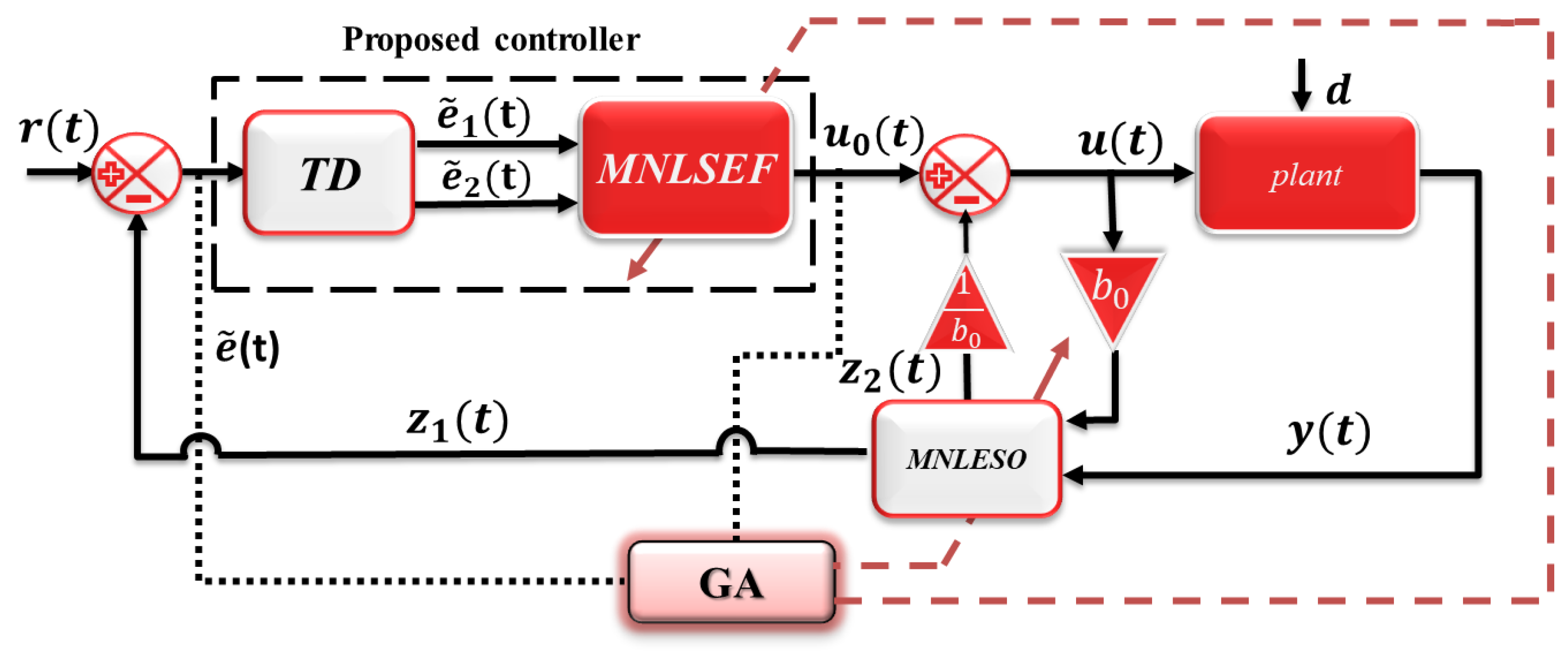
This section presents the simulation results and discussion. The four-tank model with the modified ADRC was tested and implemented using MATLAB/SIMULINK. Moreover, all the obtained results of the proposed method were compared with different methods. In this study, the genetic algorithm was utilized as an optimization technique to tune the parameters. The genetic algorithm (GA) is an optimization algorithm that was first proposed by Holland in [28]. There are three steps to generating the next generation from the current generation, the implementation of which is used to select the best generation with the best genes. Mutation is the step that generates a new offspring with a random mutation in its genes. Finally, crossover is the step that generates offspring by exchanging the genes of the parents randomly until crossover is available. In addition, the four-tank parameters used for simulation are listed in Table 4. Furthermore, a summary of all the proposed methods used in this work along with the other methods is given in Table 5. The optimization processes were achieved by means of function (GA) within the MATLAB simulation. Figure 3 shows the MADRC with GA.

Table 4. Sampled parameters of the four-tank system [1].

Parameters	Description	Value	Unit	Reference
$h_{1_{des}}$	The water level of ${\mathrm{tank}}_1$	$16$	$\mathrm{cm}$	Estimated
$h_{2_{des}}$	The water level of ${\mathrm{tank}}_2$	$13$	$\mathrm{cm}$	Estimated
$h_3$	The water level of ${\mathrm{tank}}_3$	$9.5$	$\mathrm{cm}$	Estimated
$h_4$	The water level of ${\mathrm{tank}}_4$	$6$	$\mathrm{cm}$	Estimated
$a_1$	The cross-section area of the outlet hole of ${\mathrm{tank}}_1$	$0.071$	${ \mathrm{cm}}^2$	[1]
$a_2$	The cross-section area of the outlet hole of ${\mathrm{tank}}_2$	$0.056$	${\mathrm{cm}}^2$	[1]
$a_3$	The cross-section area of the outlet hole of ${\mathrm{tank}}_3$	$0.071$	${\mathrm{cm}}^2$	[1]
$a_4$	The cross-section area of the outlet hole of ${\mathrm{tank}}_4$	$0.056$	${\mathrm{cm}}^2$	[1]
$A_1$	The cross-section area of ${\mathrm{tank}}_1$	$28$	${\mathrm{cm}}^2$	[1]
$A_2$	The cross-section area of ${\mathrm{tank}}_2$	$32$	${\mathrm{cm}}^2$	[1]
$A_3$	The cross-section area of ${\mathrm{tank}}_3$	$28$	${\mathrm{cm}}^2$	[1]
$A_4$	The cross-section area of ${\mathrm{tank}}_4$	$32$	${\mathrm{cm}}^2$	[1]
${\gamma }_1$	The ratio of the flow in the ${\mathrm{valve}}_1$	$0.7$	$\mathrm{unitless}$	[1]
${\gamma }_2$	The ratio of the flow in the ${\mathrm{valve}}_2$	$0.6$	$\mathrm{unitless}$	[1]
$k_{F{T}_1}$	Pump proportionality constant	$3.33$	$\frac{{\mathrm{cm}}^3}{\mathrm{volt}.\mathrm{s}}$	[1]
$k_{F{T}_2}$	Pump proportionality constant	$3.35$	$\frac{{\mathrm{cm}}^3}{\mathrm{volt}.\mathrm{s}}$	[1]
$g$	Gravity constant	$981$	$\mathrm{volt}/\mathrm{cm}$	[1]
$K_c$	The calibrated constant	$1$	$\mathrm{cm}/{\mathrm{s}}^2$	Estimated
$h_{max}$	The maximum height	$25$	$\mathrm{cm}$	Estimated

Table 4. Sampled parameters of the four-tank system [1].

Parameters	Description	Value	Unit	Reference
$h_{1_{des}}$	The water level of ${\mathrm{tank}}_1$	$16$	$\mathrm{cm}$	Estimated
$h_{2_{des}}$	The water level of ${\mathrm{tank}}_2$	$13$	$\mathrm{cm}$	Estimated
$h_3$	The water level of ${\mathrm{tank}}_3$	$9.5$	$\mathrm{cm}$	Estimated
$h_4$	The water level of ${\mathrm{tank}}_4$	$6$	$\mathrm{cm}$	Estimated
$a_1$	The cross-section area of the outlet hole of ${\mathrm{tank}}_1$	$0.071$	${ \mathrm{cm}}^2$	[1]
$a_2$	The cross-section area of the outlet hole of ${\mathrm{tank}}_2$	$0.056$	${\mathrm{cm}}^2$	[1]
$a_3$	The cross-section area of the outlet hole of ${\mathrm{tank}}_3$	$0.071$	${\mathrm{cm}}^2$	[1]
$a_4$	The cross-section area of the outlet hole of ${\mathrm{tank}}_4$	$0.056$	${\mathrm{cm}}^2$	[1]
$A_1$	The cross-section area of ${\mathrm{tank}}_1$	$28$	${\mathrm{cm}}^2$	[1]
$A_2$	The cross-section area of ${\mathrm{tank}}_2$	$32$	${\mathrm{cm}}^2$	[1]
$A_3$	The cross-section area of ${\mathrm{tank}}_3$	$28$	${\mathrm{cm}}^2$	[1]
$A_4$	The cross-section area of ${\mathrm{tank}}_4$	$32$	${\mathrm{cm}}^2$	[1]
${\gamma }_1$	The ratio of the flow in the ${\mathrm{valve}}_1$	$0.7$	$\mathrm{unitless}$	[1]
${\gamma }_2$	The ratio of the flow in the ${\mathrm{valve}}_2$	$0.6$	$\mathrm{unitless}$	[1]
$k_{F{T}_1}$	Pump proportionality constant	$3.33$	$\frac{{\mathrm{cm}}^3}{\mathrm{volt}.\mathrm{s}}$	[1]
$k_{F{T}_2}$	Pump proportionality constant	$3.35$	$\frac{{\mathrm{cm}}^3}{\mathrm{volt}.\mathrm{s}}$	[1]
$g$	Gravity constant	$981$	$\mathrm{volt}/\mathrm{cm}$	[1]
$K_c$	The calibrated constant	$1$	$\mathrm{cm}/{\mathrm{s}}^2$	Estimated
$h_{max}$	The maximum height	$25$	$\mathrm{cm}$	Estimated

Table 5. Summary of all the proposed methods used in this work.

Scheme	TD	SEF		ESO
Linear active disturbance rejection control LADRC	-	LPID that can be given as		Linear extended state observer (LESO) [19]
		$u_{0_{PID}}=k_p{\tilde{e}}_i+k_i{{\displaystyle \int }}_0^T{\tilde{e}}_i dt+k_d\frac{d{\tilde{e}}_i}{dt}$	(24)	$\left\{\begin{array}{c}{\dot{z}}_{i1}\left(t\right)=z_{i2}\left(t\right)+{\beta }_{i1}\left(e_i\right) \\ {\dot{z}}_{i2}\left(t\right)={\beta }_{i2}\left(e_i\right)\end{array}\right.$	(25)
ADRC	-	NLSEF [18]
		$\left\{\begin{array}{c}{u}_{0i_{NLSEF}}=fal\left({\tilde{e}}_i,{\alpha }_{i1}, {\delta }_{i1}\right)\\ fal\left({\tilde{e}}_i,{\alpha }_{i1}, {\delta }_{i1}\right)=\left\{\begin{array}{c}\frac{{\tilde{e}}_i}{ {\delta }_{i1}{}^{1-{\alpha }_{i1}}} , \left|x\right|<{\delta }_{i1}\\ {\left|{\tilde{e}}_i\right|}^{{\alpha }_{i1}}sign\left({\tilde{e}}_i\right), \left|x\right|\ge {\delta }_{i1}\end{array}\right.\end{array}\right.$	(26)
Improved active disturbance rejection control (IADRC)	-	Improved nonlinear state error feedback (INLSEF) [29]		Sliding mode extended state observer (SMESO) [30]
		$\left\{\begin{array}{c}{u}_{i1}=k_{i11}+\frac{k_{i12}}{1+\exp \left({\mu }_{i1}{\tilde{e}}_i{}^2\right)}{\left|{\tilde{e}}_i\right|}^{{\alpha }_{i1}}sign\left({\tilde{e}}_i\right)\\ u_{INLPID}=u_{i1}\end{array}\right.$	(27)	$\left\{\begin{array}{c}{\dot{z}}_{i1}\left(t\right)=z_{i2}\left(t\right)+{\beta }_{i1}\left(k\left(e_i\left(t\right)\right)e_i\left(t\right)\right)\\ {\dot{z}}_{i2}\left(t\right)={\beta }_{i1}(k\left(e_i\left(t\right)\right)e_i\left(t\right)\\ k\left(e_i\left(t\right)\right)=k_{{\alpha }_i}{\left|e_i\right|}^{{\alpha }_i-1}+k_{\beta }{\left|e_i\right|}^{{\beta }_i}\end{array}\right.$	(28)
		$\mathrm{where} {\tilde{e}}_i$$\mathrm{is} \mathrm{the} \mathrm{error} \mathrm{and} (k_{i11},k_{i12}, {\mu }_{i1},{\alpha }_{i1}$) are the controller parameters		$\mathrm{where} k\left(e_i\left(t\right)\right)$ is a nonlinear function
S fal-ADRC	-	NLSEF Equation (26)		Symmetrical fal ESO Equation (11)
D fal-ADRC	-			Different fal ESO Equation (12)
$1\mathrm{st}$ MADRC scheme (NLP-ADRC) and (STC-ADRC)	Equation (3a)	Proposed NLPD Equation (5)		$\mathrm{MNLESO} 1\mathrm{st}$ scheme Equation (7)
	Equation (3b)	Proposed STC-SM Equation (6)		$\mathrm{MNLESO} 2\mathrm{nd}$ scheme Equation (8)
$2\mathrm{nd}$ MADRC scheme (D fal-ADRC-TD)	Equation (8)	Proposed MNLSEF Equations (9) and (10)		Different fal ESO Equation (12)

Table 5. Summary of all the proposed methods used in this work.

Scheme	TD	SEF		ESO
Linear active disturbance rejection control LADRC	-	LPID that can be given as		Linear extended state observer (LESO) [19]
		$u_{0_{PID}}=k_p{\tilde{e}}_i+k_i{{\displaystyle \int }}_0^T{\tilde{e}}_i dt+k_d\frac{d{\tilde{e}}_i}{dt}$	(24)	$\left\{\begin{array}{c}{\dot{z}}_{i1}\left(t\right)=z_{i2}\left(t\right)+{\beta }_{i1}\left(e_i\right) \\ {\dot{z}}_{i2}\left(t\right)={\beta }_{i2}\left(e_i\right)\end{array}\right.$	(25)
ADRC	-	NLSEF [18]
		$\left\{\begin{array}{c}{u}_{0i_{NLSEF}}=fal\left({\tilde{e}}_i,{\alpha }_{i1}, {\delta }_{i1}\right)\\ fal\left({\tilde{e}}_i,{\alpha }_{i1}, {\delta }_{i1}\right)=\left\{\begin{array}{c}\frac{{\tilde{e}}_i}{ {\delta }_{i1}{}^{1-{\alpha }_{i1}}} , \left|x\right|<{\delta }_{i1}\\ {\left|{\tilde{e}}_i\right|}^{{\alpha }_{i1}}sign\left({\tilde{e}}_i\right), \left|x\right|\ge {\delta }_{i1}\end{array}\right.\end{array}\right.$	(26)
Improved active disturbance rejection control (IADRC)	-	Improved nonlinear state error feedback (INLSEF) [29]		Sliding mode extended state observer (SMESO) [30]
		$\left\{\begin{array}{c}{u}_{i1}=k_{i11}+\frac{k_{i12}}{1+\exp \left({\mu }_{i1}{\tilde{e}}_i{}^2\right)}{\left|{\tilde{e}}_i\right|}^{{\alpha }_{i1}}sign\left({\tilde{e}}_i\right)\\ u_{INLPID}=u_{i1}\end{array}\right.$	(27)	$\left\{\begin{array}{c}{\dot{z}}_{i1}\left(t\right)=z_{i2}\left(t\right)+{\beta }_{i1}\left(k\left(e_i\left(t\right)\right)e_i\left(t\right)\right)\\ {\dot{z}}_{i2}\left(t\right)={\beta }_{i1}(k\left(e_i\left(t\right)\right)e_i\left(t\right)\\ k\left(e_i\left(t\right)\right)=k_{{\alpha }_i}{\left|e_i\right|}^{{\alpha }_i-1}+k_{\beta }{\left|e_i\right|}^{{\beta }_i}\end{array}\right.$	(28)
		$\mathrm{where} {\tilde{e}}_i$$\mathrm{is} \mathrm{the} \mathrm{error} \mathrm{and} (k_{i11},k_{i12}, {\mu }_{i1},{\alpha }_{i1}$) are the controller parameters		$\mathrm{where} k\left(e_i\left(t\right)\right)$ is a nonlinear function
S fal-ADRC	-	NLSEF Equation (26)		Symmetrical fal ESO Equation (11)
D fal-ADRC	-			Different fal ESO Equation (12)
$1\mathrm{st}$ MADRC scheme (NLP-ADRC) and (STC-ADRC)	Equation (3a)	Proposed NLPD Equation (5)		$\mathrm{MNLESO} 1\mathrm{st}$ scheme Equation (7)
	Equation (3b)	Proposed STC-SM Equation (6)		$\mathrm{MNLESO} 2\mathrm{nd}$ scheme Equation (8)
$2\mathrm{nd}$ MADRC scheme (D fal-ADRC-TD)	Equation (8)	Proposed MNLSEF Equations (9) and (10)		Different fal ESO Equation (12)

The multi-objective performance index (OPI) was used in this work to tune the parameters of the modified ADRC (MADRC) and the methods in Table 4 in order to find the optimal value. It is expressed as follows:

$$\left\{\begin{array}{c}OP{I}_1={𝓌}_{11}\times \frac{ITA{E}_1}{{\mathcal{N}}_{11}}+{𝓌}_{12}\times \frac{IA{U}_1}{{\mathcal{N}}_{12}}+{𝓌}_{13}\times \frac{IS{U}_2}{{\mathcal{N}}_{13}}\\ OP{I}_2={𝓌}_{21}\times \frac{ITA{E}_2}{{\mathcal{N}}_{21}}+{𝓌}_{22}\times \frac{IA{U}_2}{{\mathcal{N}}_{22}}+{𝓌}_{32}\times \frac{IS{U}_2}{{\mathcal{N}}_{23}}\\ OPI={\mathcal{W}}_1\times OP{I}_1+{\mathcal{W}}_2\times OP{I}_2\end{array}\right.$$

(29)

The value of ${\mathcal{W}}_1$ and ${\mathcal{W}}_2$ were set to $0.5,$ and the weighted factor of each subsystem was set to ${𝓌}_{11}={𝓌}_{21}=0.4,$ ${𝓌}_{12}={𝓌}_{22}=0.2,$ ${𝓌}_{13}={𝓌}_{23}=0.4$. The nominal values of the individual objectives that contain the (OPI) were set to ${\mathcal{N}}_{11}=1.814362,$ ${\mathcal{N}}_{12}=4389.20,$ ${\mathcal{N}}_{13}=305.59,$ ${\mathcal{N}}_{21}=1.77746,$ ${\mathcal{N}}_{22}=4332.233$, and ${\mathcal{N}}_{23}=285.2937$. After the tuning process was conducted using GA [31,32], the parameter values of the modified ADRC and all the methods mentioned previously in Table 5 were obtained and are given in

Table 6. LADRC parameters.

ADRC Parts	Parameter	Value	Parameter	Value
LPID	$k_{p_1}$	$18.6300$	$k_{p_2}$	$26.6550$
	$k_{i_1}$	$0.0002$	$k_{i_2}$	$0.0024$
	$k_{d_1}$	$2.5300$	$k_{d_2}$	$3.0500$
LESO	${\omega }_{01}$	$43.130000$	${\omega }_{02}$	$15.910000$
	$b_{01}$	$0.124875$	$b_{02}$	$0.094219$

,

Table 7. ADRC parameters.

ADRC Parts	Parameter	Value	Parameter	Value
NLSEF	${\alpha }_1$	$0.7763$	${\alpha }_2$	$0.4167$
	${\delta }_1$	$0.0140$	${\delta }_2$	$1.8958$
LESO	${\omega }_{01}$	$149.345000$	${\omega }_{02}$	$173.005000$
	$b_{01}$	$1.706625$	$b_{02}$	$1.287656$

,

Table 8. IADRC parameters.

ADRC Parts	Parameter	Value	Parameter	Value
INLP (INSEF)	$k_{111}$	$6.2650$	$k_{212}$	$7.0400$
	$k_{121}$	$1.4124$	$k_{222}$	$0.0142$
	${\mu }_{11}$	$8.5790$	${\mu }_{22}$	$5.6130$
	${\alpha }_{11}$	$0.6812$	${\alpha }_{22}$	$0.6625$
SMESO	$k_{{\alpha }_1}$	$0.3675$	$k_{{\alpha }_2}$	$0.8579$
	${\alpha }_1$	$0.9733$	${\alpha }_2$	$0.6265$
	$k_{{\beta }_1}$	$0.6713$	$k_{{\beta }_2}$	$0.6812$
	${\beta }_1$	$0.2221$	${\beta }_2$	$0.7062$
	${\omega }_{01}$	$133.200000$	${\omega }_{02}$	$163.840000$
	$b_{01}$	$0.666000$	$b_{02}$	$0.502500$

,

Table 9. NLPD-ADRC parameters ($1\mathrm{st}$ MADRC scheme).

ADRC Parts	Parameter	Value	Parameter	Value
NLPD	$k_{11}$	$12.676500$	$k_{12}$	$24.414000$
	${\mathsf{\alpha }}_{11}$	$0.351000$	${\mathsf{\alpha }}_{12}$	$0.453100$
	$k_{21}$	$22.057500$	$k_{22}$	$21.553500$
	${\mathsf{\alpha }}_{21}$	$0.931500$	${\mathsf{\alpha }}_{22}$	$0.69130$
TD	$R$	$55.380000$	$a_2$	$7.842000$
	$a_1$	$0.142000$	$-$	$-$
$1st$ MNLESO scheme	${\omega }_{01}$	$341.190000$	${\omega }_{02}$	$538.050000$
	${𝒶}_1$	$0.696800$	${𝒶}_2$	$0.587100$
	$b_{01}$	$2.414250$	$b_{02}$	$1.821562$

,

Table 10. STC-ADRC parameters ($1\mathrm{st}$ MADRC scheme).

ADRC Parts	Parameter	Value	Parameter	Value
STC-SM	${\kappa }_1$	$0.552000$	${\kappa }_2$	$0.587800$
	${\xi }_1$	$3.405000$	${\xi }_2$	$3.889500$
	${𝓅}_1$	$0.704480$	${𝓅}_2$	$0.695040$
	$\delta$	$7.631000$	$-$	$-$
TD	$R$	$188.580000$	$a_2$	$3.896000$
	$a_1$	$3.052000$	$-$	$-$
NLESO	${\omega }_{01}$	$103.000000$	${\omega }_{02}$	$80.300000$
	${𝒶}_1$	$0.905498$	${𝒶}_2$	$0.873169$
	${\mathcal{A}}_1$	$0.524300$	${\mathcal{A}}_2$	$0.102500$
	$b_{01}$	$3.230100$	$b_{02}$	$2.688375$

,

Table 11. S$fal$ -ADRC parameters.

ADRC Parts	Parameter	Value	Parameter	Value
NLSEF	${\alpha }_1$	$0.962100$	${\alpha }_2$	$0.542400$
	${\delta }_1$	$0.532800$	${\delta }_2$	$0.693800$
S-$fal$	${\alpha }_{1_{ESO}}$	$0.097200$	${\alpha }_{2_{ESO}}$	$0.547200$
	${\delta }_{1_{ESO}}$	$0.765600$	${\delta }_{2_{ESO}}$	$0.369000$
LESO	${\omega }_{01}$	$261.300000$	${\omega }_{02}$	$224.220000$
	$b_{01}$	$1.914750$	$b_{02}$	$1.444687$

,

Table 12. D$fal$ -ADRC parameters.

ADRC Parts	Parameter	Value	Parameter	Value
NLSEF	${\alpha }_1$	$0.962900$	${\alpha }_2$	$0.968200$
	${\delta }_1$	$0.910600$	${\delta }_2$	$0.139200$
D-$fal$	${\alpha }_{{11}_{ESO}}$	$0.151200$	${\alpha }_{{21}_{ESO}}$	$0.443600$
	${\delta }_{{11}_{ESO}}$	$0.903800$	${\delta }_{{21}_{ESO}}$	$0.217900$
	${\alpha }_{{12}_{ESO}}$	$0.066200$	${\alpha }_{{22}_{ESO}}$	$0.045300$
	${\delta }_{{12}_{ESO}}$	$0.485300$	${\delta }_{{22}_{ESO}}$	$0.024700$
LESO	${\omega }_{01}$	$230.430000$	${\omega }_{02}$	$266.220000$
	$b_{01}$	$2.289375$	$b_{02}$	$2.167031$

and

Table 13. D$fal$ -ADRC-TD parameters ($2\mathrm{nd}$ MADRC scheme).

ADRC Parts	Parameter	Value	Parameter	Value
MNLSEF	${\alpha }_{11}$	$0.802800$	${\alpha }_{21}$	$0.646400$
	${\delta }_{11}$	$0.277500$	${\delta }_{21}$	$0.090400$
	${\alpha }_{12}$	$0.170300$	${\alpha }_{22}$	$0.698500$
	${\delta }_{12}$	$0.457400$	${\delta }_{22}$	$0.153900$
TD	$R$	$6.050000$	$a_2$	$13.404000$
	$a_1$	$0.887000$	$-$	$-$
D-$fal$	${\alpha }_{{11}_{ESO}}$	$0.843900$	${\alpha }_{{21}_{ESO}}$	$0.724800$
	${\delta }_{{11}_{ESO}}$	$0.521700$	${\delta }_{{21}_{ESO}}$	$0.634300$
	${\alpha }_{{12}_{ESO}}$	$0.231600$	${\alpha }_{{21}_{ESO}}$	$0.141500$
	${\delta }_{{12}_{ESO}}$	$0.023300$	${\delta }_{{21}_{ESO}}$	$0.086500$
LESO	${\omega }_{01}$	$183.570000$	${\omega }_{02}$	$292.230000$
	$b_{01}$	$4.620375$	$b_{02}$	$3.548906$

.

To check the effectiveness of the proposed method, three tests were applied to the four-tank model as follows:

A.

Case study 1. Exogenous disturbance

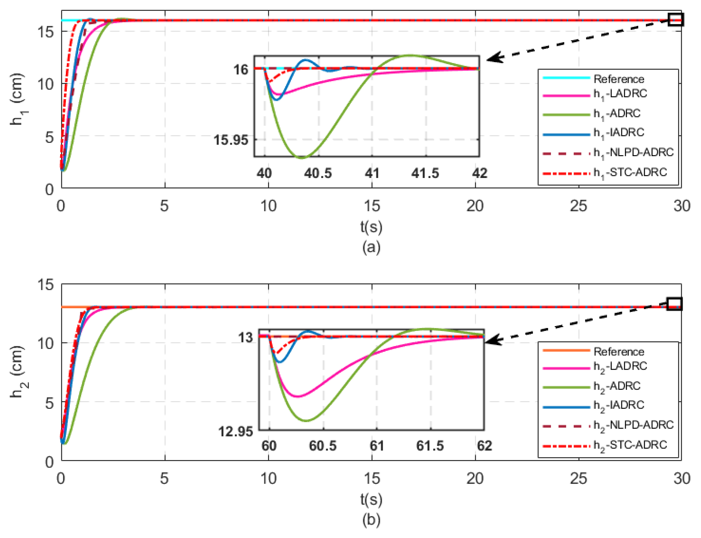
In this test, a step function was applied as a desired reference for both subsystems. Moreover, to investigate the effectiveness and robustness of the designed ADRC against the applied disturbance, a step function was applied as an exogenous disturbance. The water levels of both subsystems while applying an exogenous disturbance after $40 \mathrm{s}$ of starting the simulation for the first subsystem and after $60 \mathrm{s}$ of starting the simulation for the second subsystem are shown in Figure 4. The output response of the first subsystem is given in Figure 4a. The results show that in applying disturbance for the first subsystem at $t=40 \mathrm{s}$, LADRC, ADRC, and IADRC exhibited an output response with an undershoot which reached nearly $0.1265\%$, $0.375\%$, $0.1875\%$, and $0.125\%$ of the steady-state value, respectively, and lasted about $1.2 \mathrm{s}$ for LADRC, $2.1 \mathrm{s}$ for ADRC, and $0.5 \mathrm{s}$ for IADRC until the output response reached its steady state. For the second subsystem as shown in Figure 4b, at $t=60s$ the output response exhibited an undershoot which reached nearly $0.307\%$, $0.315\%$, and $0.153\%$ of its steady-state value for LADRC, ADRC and IADRC, respectively, and lasted about $1.9 \mathrm{s}$ for LADRC, $1.92 \mathrm{s}$ for ADRC, and $0.5 \mathrm{s}$ for IADRC until it reached its steady state. However, the proposed methods rejected the disturbance very quickly. It is observed that the output response of the proposed methods (i.e., NLPD-ADRC, STC-ADRC) is faster, smoother, and without overshooting when compared with the other methods. It took less than approximately $2 \mathrm{s}$ to reach the steady state (desired value), while a longer settling time was clearly observed in the output responses of the other methods.

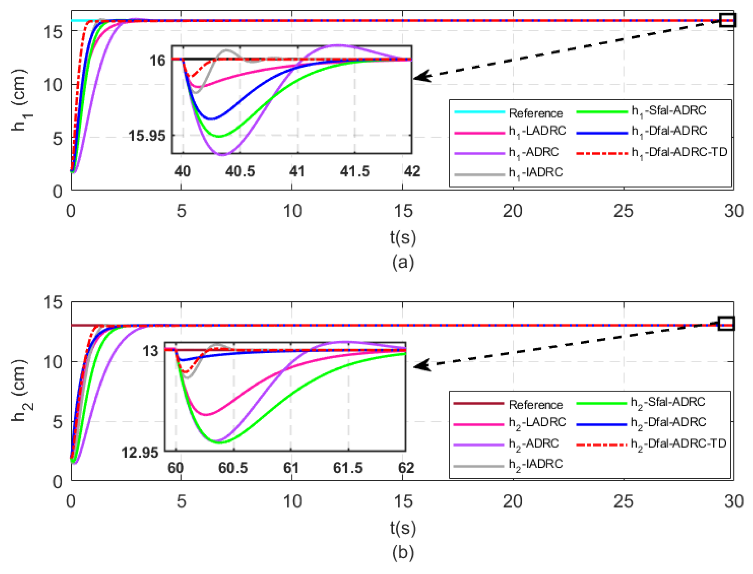
The output response when using the second MADRC scheme is shown in Figure 5. As can be seen from Figure 5a, the output response reached a steady state with a smooth and fast response. However, it took approximately $1 \mathrm{s}$ and $1.5 \mathrm{s}$ for S$fal$-ADRC and D$fal$-ADRC to attenuate the disturbance and return to the steady state, respectively. Furthermore, under the effect of the disturbance, the output showed an undershoot of $0.3125\%$ and $0.25\%$ of the steady state value for S$fal$-ADRC and D$fal$-ADRC, respectively. By contrast, the output response of the proposed method (i.e., D$fal$-ADRC-TD) is smooth and more accurate, representing an improvement in terms of disturbance attenuation compared with D$fal$-ADRC and S$fal$-ADRC, which proves the effectiveness of the designed controller and observer. Further, as can be seen from Figure 5b, the output response of the proposed method (i.e., D$fal$-ADRC-TD) under the disturbance effect shows an improvement and robustness in canceling the disturbance effect in a short time, while the other methods, LADRC, ADRC, and S$fal$-ADRC, take about $1.9 \mathrm{s}$, $1.92 \mathrm{s}$, and $2 \mathrm{s}$ to remove the disturbance effect and return to the steady state, respectively. Moreover, the output responses of the methods under the effect of the disturbance showed an undershoot of $0.307\%$, $0.315\%$, $0.305\%$, $0.153\%$, and $0.315\%$ of the steady-state value for LADRC, ADRC, IADRC, and S$fal$-ADRC, respectively.

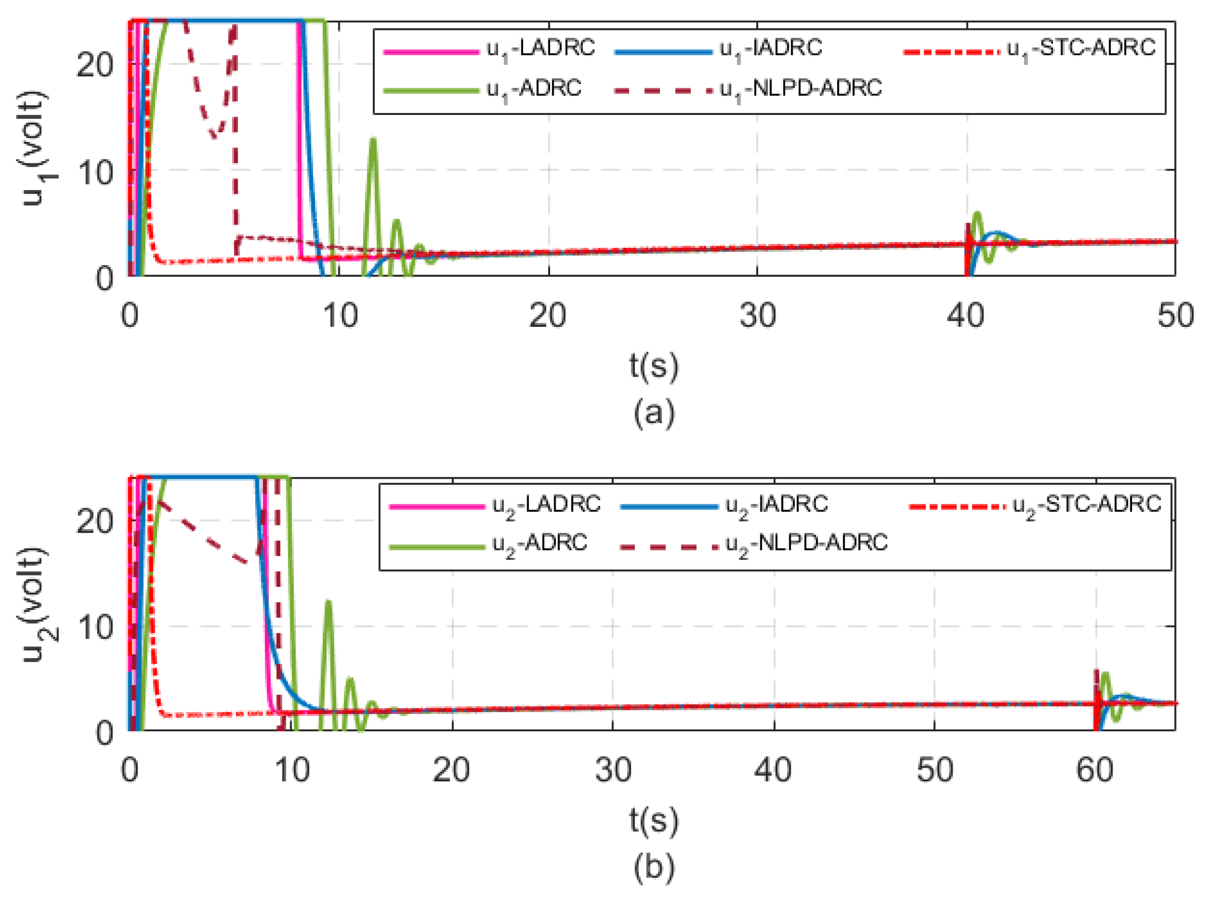
Figure 6a,b show the control signal of the first subsystem and the second subsystem respectively. It is observed that the first MADRC scheme (i.e., STC-ADRC) is chattering-free with a smooth response; moreover, the NLPD-ADRC shows a reduction in chattering, while the other methods, such as ADRC, show chattering in the control signal. This proves the effectiveness of the proposed method.

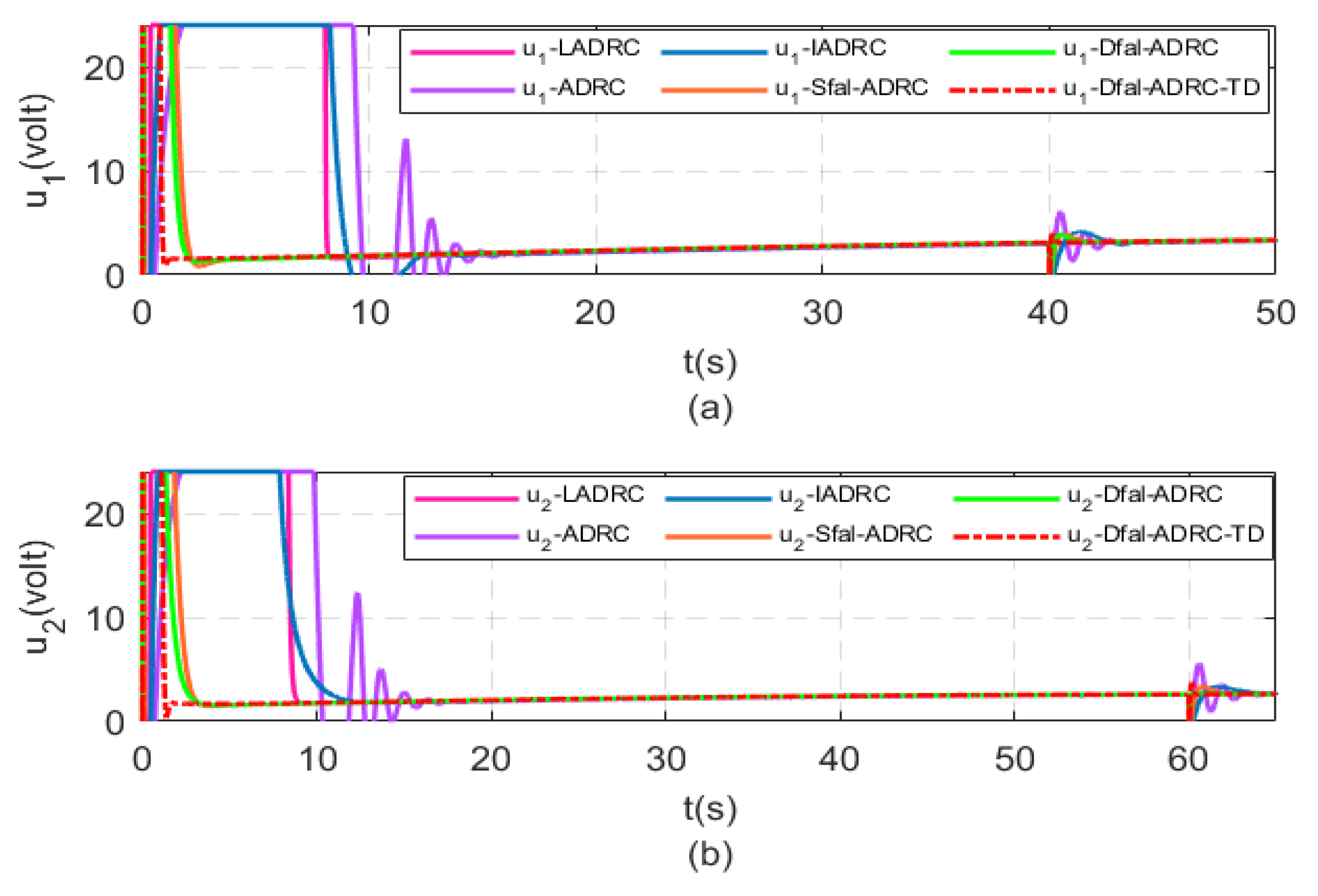
Figure 7a,b show the control signal of the first subsystem and the second subsystem, respectively. It is observed that the second MADRC scheme (i.e., D$fal$-ADRC-TD) is chattering-free with a smooth response, while the other methods, such as ADRC, show chattering in the control signal. This proves the effectiveness of the proposed method.

B.

Case study 2. Parameter uncertainty

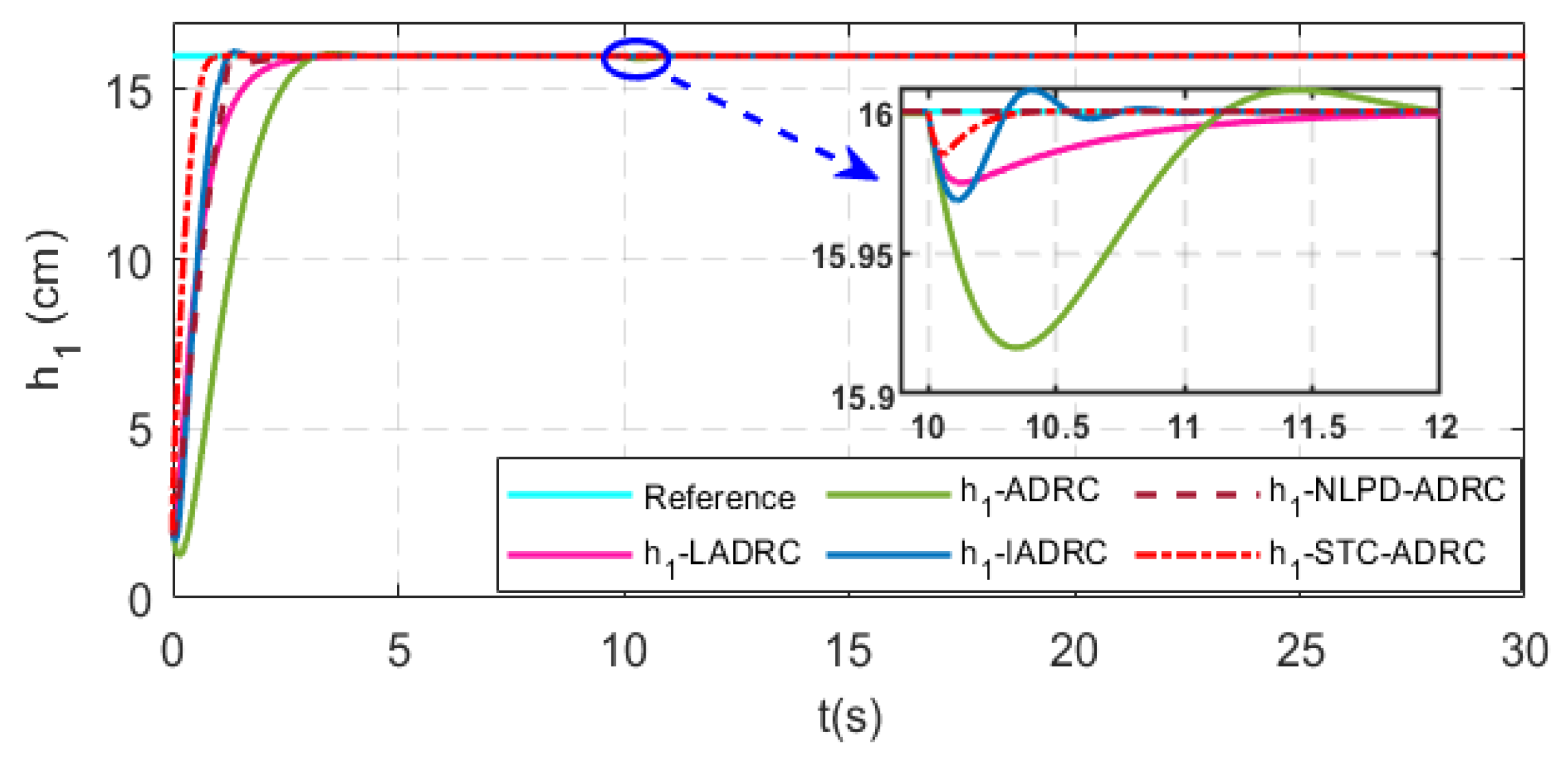
In this test, the system’s parameter uncertainty is taken into consideration to observe its effect on the nonlinear system. One of the parameters that affects the performance of the four-tank model is uncertainty in the design of the outlet hole of the first tank. Figure 8 show the output response of the first tank under the presence of the parameter uncertainties (${\Delta }_{{\mathrm{a}}_1}=+9\%$) after $10 \mathrm{s}$ from starting the simulation. It appears that the proposed methods (i.e., NLPD-ADRC, STC-ADRC) can cope with parameter variation easily, while the other methods give undershoots of $0.1875\%,0.5\%, 0.31255\% \mathrm{and} 0.5\%$ of the steady state, respectively, and it takes LADRC, ADRC, and IADRC approximately $1.95 \mathrm{s}, 2.96 \mathrm{s}, 1.07 \mathrm{s}, \mathrm{and} 1.04 \mathrm{s}$ to weaken and reduce the uncertainty effect, respectively. By contrast, the proposed methods attenuate the effect of the parameter variation in less than $1 \mathrm{s}$.

C.

Case study 3. Reference tracking

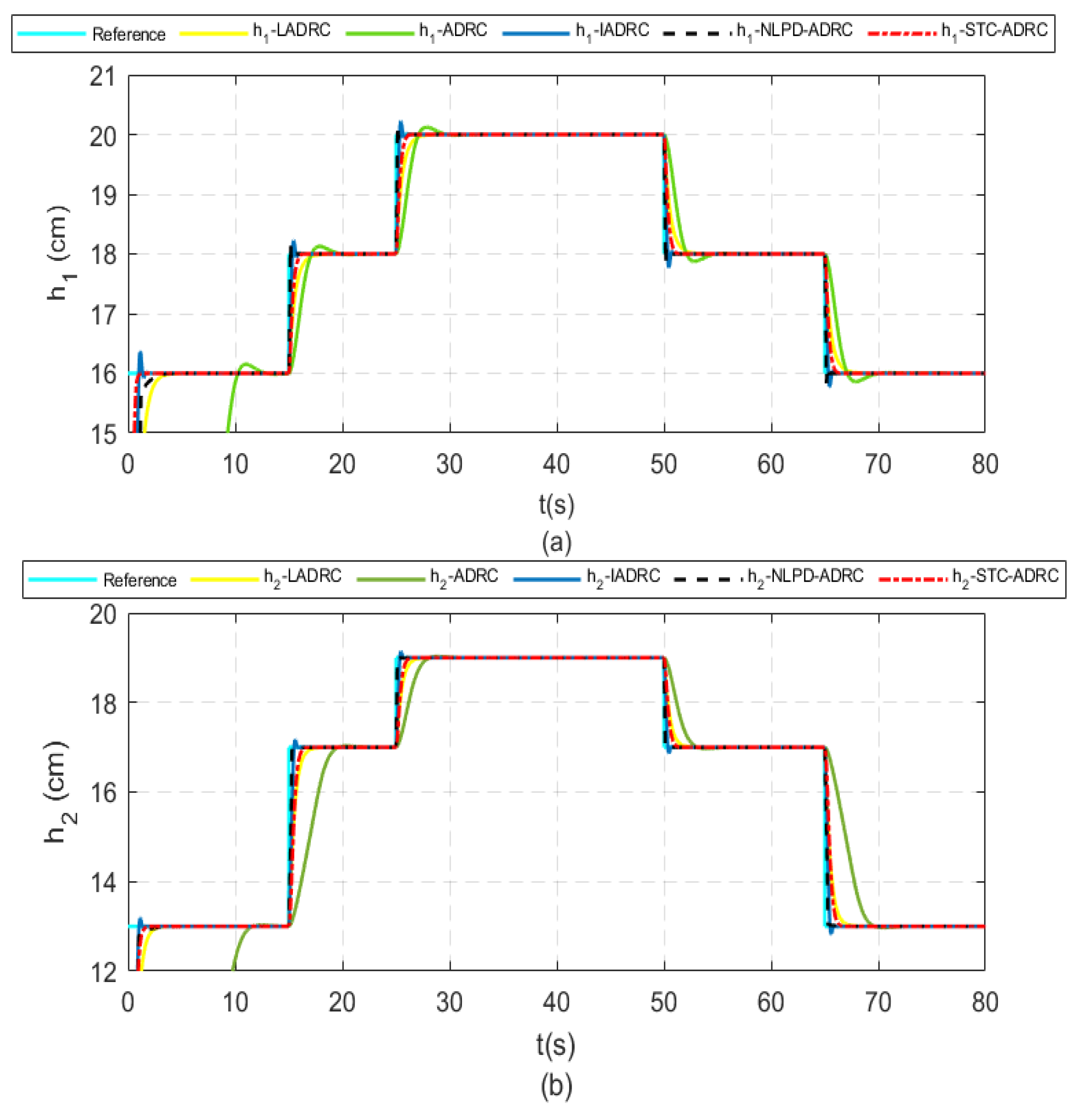
In this test, a step function was applied for both subsystems with different amplitude and time to check the robustness and validation of the designed MNLESO and controllers in tracking references applied at different times.

Figure 9a shows the output response of the first subsystem when using NLPD-ADRC and STC-ADRC, while Figure 9b shows the output response of the second subsystem. It is clear for both subsystems that the proposed methods (i.e., NLPD-ADRC and STC-ADRC) exhibit a smooth, fast-tracking, chattering-free, and accurate response without any visible over or undershoot (STC-ADRC), which reflects the effectiveness of the designed ESO and controller in coping with the time-varying reference.

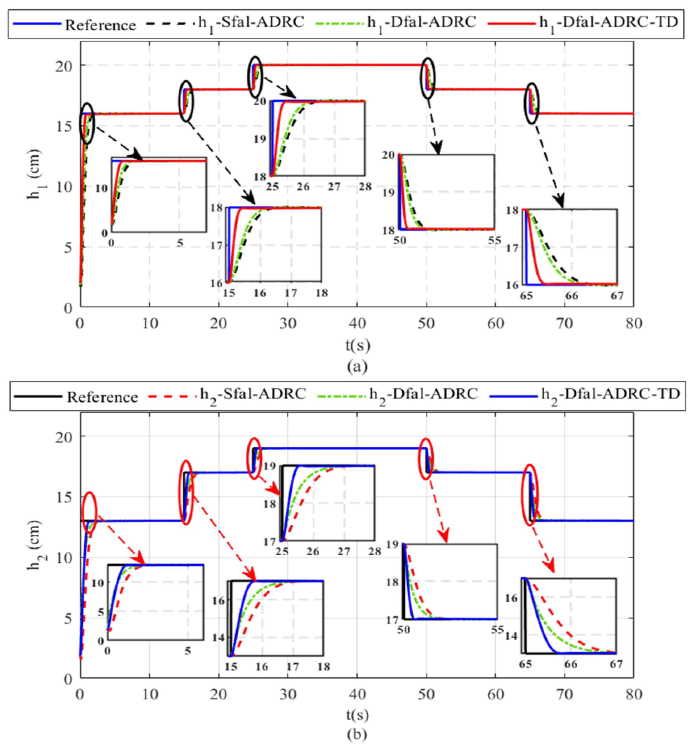
Figure 10a shows the output response of the first subsystem when using S$fal$-ADRC, D$fal$-ADRC, and D$fal$-ADRC-TD, while Figure 10b shows the output response of the second subsystem. It is clear for both subsystems that the proposed method (D$fal$-ADRC-TD) exhibits a smooth, fast-tracking, and accurate response without any peaking, which proves the effectiveness of the designed ESO and controller under the time-varying references.

Table 14. Performance indices.

PI	$\mathit{I}\mathit{T}\mathit{A}{\mathit{E}}_1$	$\mathit{I}\mathit{T}\mathit{A}{\mathit{E}}_2$	$\mathit{I}\mathit{A}{\mathit{U}}_1$	$\mathit{I}\mathit{A}{\mathit{U}}_2$	$\mathit{I}\mathit{S}{\mathit{U}}_1$	$\mathit{I}\mathit{S}{\mathit{U}}_2$	$\mathit{O}\mathit{P}\mathit{I}$
LADRC	$5.0488$	$7.5142$	$13115.098$	$16124.001$	$16194.336$	$20840.561$	$23.2190$
ADRC	$10.7318$	$13.4633$	$976.4132$	$1021.5292$	$54.0156$	$46.700165$	$2.48116$
IADRC	$2.6097$	$2.6842$	$2518.480536$	$2695.5036$	$678.3466$	$658.7566$	$1.578022$
$\mathrm{S}fal-\mathrm{ADRC}$	$3.8810$	$5.5178$	$850.1411$	$908.2580$	$75.9051$	$64.6534$	$0.993720$
$\mathrm{D}fal-\mathrm{ADRC}$	$2.5716$	$2.4849$	$682.9920$	$528.7538$	$59.2170$	$29.5555$	$0.675591$
$\mathrm{D}fal-\mathrm{ADRC}-\mathrm{TD}$	$2.2750$	$2.5949$	$350.4789$	$328.2163$	$21.8594$	$12.0197$	$0.546157$
$\mathrm{NLPD}-\mathrm{ADRC}$	$3.7407$	$2.2867$	$635.1552$	$696.2649$	$30.7188$	$37.6227$	$0.893849$
$\mathrm{STC}-\mathrm{ADRC}$	$0.714658$	$1.8739$	$289.7189$	$426.9655$	$32.3728$	$22.6835$	$0.213131$

below proves that the STC-ADRC method provides the best result in terms of OPI reduction and steady-state error, while the other methods, such as NLPD-TD, D fal-ADRC, and D fal-ADRC-TD exhibit noticeable reduction in the OPI.

Remark 1.

The intelligent PID (iPID) is a PID controller where the nonlinearity, unknown parts of the plant, and time-varying parameters are considered but do not appear in the modeling (see [33]). The ADRC is a robust control which estimates the total disturbance and rejects it in an online manner (see, for example, Equation (7) and [18,20,21]).

7. Conclusions

Two MADRC schemes were proposed in this paper with the nonlinear model of the four-tank system and under different conditions such as exogenous disturbance, parameter uncertainty, and reference tracking. The first MADRC scheme was designed using the STC-SM and NLPD with an NLESO and the proposed TD. The simulation results showed the robustness of the first MADRC scheme (i.e., STC-ADRC and NLPD-ADRC) in terms of disturbance and uncertainty reduction and the desired output tracking. Another modified ADRC scheme (i.e., second MADRC scheme) was also proposed with NLSEF-TD as a new controller and a new NLSEO using the $fal$ as a nonlinear function. In conclusion, the simulation results of the proposed method (i.e., D$fal$-ADRC-TD) exhibited better results in terms of disturbance cancelation and output response performance with minimum OPI compared with both S$fal$-ADRC and D$fal$-ADRC. Finally, with respect to future work, we intend to extend the current work by including delays in the four-tank system and a condition wherein the four-tank system operates in the non-minimum phase mode.

References

1. Johansson, K.H. The quadruple-tank process: A multivariable laboratory process with an adjustable zero. IEEE Trans. Control. Syst. Technol. 2000, 8, 456–465. [Google Scholar] [CrossRef]
2. Johansson, K.H.; Nunes, J.L.R. A multivariable laboratory process with an adjustable zero. In Proceedings of the 1998 American Control Conference. ACC (IEEE Cat. No. 98CH36207), Philadelphia, PA, USA, 26 June 1998; Volume 4, pp. 2045–2049. [Google Scholar] [CrossRef]
3. Altabey, W.A. Model Optimal Control of the Four Tank System. Int. J. Syst. Sci. Appl. Math. 2016, 1, 30–41. [Google Scholar]
4. Sorcia-Vázquez, F.; García-Beltrán, C.; Valencia-Palomo, G.; Brizuela-Mendoza, J.; Rumbo-Morales, J. Decentralized robust tube-based model predictive control: Application to a four-tank-system. Rev. Mex. Ing. Química 2020, 19, 1135–1151. [Google Scholar] [CrossRef]
5. Chaudhari, V.; Tamhane, B.; Kurode, S. Robust Liquid Level Control of Quadruple Tank System-Second Order Sliding Mode. IFAC Pap. OnLine 2020, 53, 7–12. [Google Scholar] [CrossRef]
6. Osman, A.; Kara, T.; Arıcı, M. Robust Adaptive Control of a Quadruple Tank Process with Sliding Mode and Pole Placement Control Strategies. IETE J. Res. 2021. [Google Scholar] [CrossRef]
7. Biswas, P.P.; Srivastava, R.; Ray, S.; Samanta, A.N. Sliding mode control of quadruple tank process. Mechatronics 2009, 19, 548–561. [Google Scholar] [CrossRef]
8. Shah, D.H.; Patel, D.M. Design of sliding mode control for quadruple-tank MIMO process with time delay compensation. J. Process Control 2019, 76, 46–61. [Google Scholar] [CrossRef]
9. Thamallah, A.; Sakly, A.; M’Sahli, F. A new constrained PSO for fuzzy predictive control of Quadruple-Tank process. Measurement 2018, 136, 93–104. [Google Scholar] [CrossRef]
10. Eltantawie, M.A. Decentralized neuro-fuzzy controllers of nonlinear quadruple tank system. SN Appl. Sci. 2018, 1, 39. [Google Scholar] [CrossRef]
11. Son, N.N. Level Control of Quadruple Tank System Based on Adaptive Inverse Evolutionary Neural Controller. Int. J. Control Autom. Syst. 2020, 18, 2386–2397. [Google Scholar] [CrossRef]
12. Naami, G.; Ouahi, M.; Rabhi, A.; Tadeo, F.; Tuan, V.L.B. Design of robust control for uncertain fuzzy quadruple-tank systems with time-varying delays. Granul. Comput. 2022, 7, 951–964. [Google Scholar] [CrossRef]
13. Meng, X.; Yu, H.; Xu, T.; Wu, H. Sliding mode disturbance observer-based the port-controlled Hamiltonian control for a four-tank liquid level system subject to external disturbances. In Proceedings of the Chinese Control and Decision Conference (CCDC), Hefei, China, 22–24 August 2020; pp. 1720–1725. [Google Scholar] [CrossRef]
14. Meng, X.; Yu, H.; Zhang, J.; Xu, T.; Wu, H.; Yan, K. Disturbance Observer-Based Feedback Linearization Control for a Quadruple-Tank Liquid Level System. ISA Trans. 2022, 122, 146–162. [Google Scholar] [CrossRef] [PubMed]
15. Gurjar, B.; Chaudhari, V.; Kurode, S. Parameter estimation based robust liquid level control of quadruple tank system -Second order sliding mode approach. J. Process Control 2021, 104, 1–10. [Google Scholar] [CrossRef]
16. Meng, X.; Yu, H.; Zhang, J.; Xu, T.; Wu, H. Liquid Level Control of Four-Tank System Based on Active Disturbance Rejection Technology. Measurement 2021, 175, 109146. [Google Scholar] [CrossRef]
17. Huang, C.; Canuto, M.E.; Novara, C. The four-tank control problem: Comparison of two disturbance rejection control solutions. ISA Trans. 2017, 71, 252–271. [Google Scholar] [CrossRef] [PubMed]
18. Han, J. From PID to Active Disturbance Rejection Control. IEEE Trans. Ind. Electron. 2009, 56, 900–906. [Google Scholar] [CrossRef]
19. Yoo, D.; Yau, S.S.T.; Gao, Z. On convergence of the linear extended state observer. In Proceedings of the 2006 IEEE Conference on Computer Aided Control System Design, 2006 IEEE International Conference on Control Applications, 2006 IEEE International Symposium on Intelligent Control, Munich, Germany, 4–6 October 2006; pp. 1645–1650. [Google Scholar] [CrossRef]
20. Sira-Ramírez, H.; Luviano-Juárez, A.; Ramírez-Neria, M.; Zurita-Bustamante, E.W. Active Disturbance Rejection Control of Dynamic Systems: A Flatness-Based Approach; Butterworth-Heinemann: Oxford, UK, 2017. [Google Scholar]
21. Guo, B.Z.; Zhao, Z. Active Disturbance Rejection Control for Nonlinear Systems: An Introduction; John Wiley & Sons: New York, NY, USA, 2017. [Google Scholar]
22. Najm, A.A.; Ibraheem, I.K. Altitude and attitude stabilization of UAV quadrotor system using improved active disturbance rejection control. Arab. J. Sci. Eng. 2020, 45, 1985–1999. [Google Scholar] [CrossRef]
23. Hou, G.; Ke, Y.; Huang, C. A flexible constant power generation scheme for photovoltaic system by error-based active disturbance rejection control and perturb & observe. Energy 2021, 237, 121646. [Google Scholar] [CrossRef]
24. Abdul-Adheem, W.R.; Ibraheem, I.K.; Humaidi, A.J.; Alkhayyat, A.; Maher, R.A.; Abdulkareem, A.I.; Azar, A.T. Design and Analysis of a Novel Generalized Continuous Tracking Differentiator. Ain Shams Eng. J. 2021, 13, 101656. [Google Scholar] [CrossRef]
25. Guo, B.Z.; Zhao, Z.L. On the convergence of an extended state observer for nonlinear systems with uncertainty. Syst. Control Lett. 2011, 60, 420–430. [Google Scholar] [CrossRef]
26. Khalil, K.H. Nonlinear Control; Global Edition; Pearson Education: London, UK, 2015. [Google Scholar]
27. Anton, H.; Bivens, I.C.; Davis, S. Calculus, 11th ed.; John Wiley & Sons: New York, NY, USA, 2020. [Google Scholar]
28. Holland, J. Adaptation in Natural and Artificial Systems; University of Michigan Press: Ann Arbor, MI, USA, 1975. [Google Scholar]
29. Abdul-Adheem, W.R.; Ibraheem, I.K. From PID to Nonlinear State Error Feedback Controller. Int. J. Adv. Comput. Sci. Appl. 2017, 8, 312–322. [Google Scholar] [CrossRef]
30. Abdul-Adheem, W.R.; Ibraheem, I.K. Improved Sliding Mode Nonlinear Extended State Observer based Active Disturbance Rejection Control for Uncertain Systems with Unknown Total Disturbance. Int. J. Adv. Comput. Sci. Appl. 2016, 7, 80–93. [Google Scholar] [CrossRef]
31. Najm, A.A.; Ibraheem, I.K.; Azar, A.T.; Humaidi, A. Genetic optimization-based consensus control of multi-agent 6-DoF UAV system. Sensors 2020, 20, 3576. [Google Scholar] [CrossRef] [PubMed]
32. Aziz, A.S.A.; Hassanien, A.E.; Azar, A.T.; Hanafy, S.E. Genetic Algorithm with Different Feature Selection Techniques for Anomaly Detectors Generation. In Proceedings of the 2013 Federated Conference on Computer Science and Information Systems (FedCSIS), Kraków, Poland, 8–11 September 2013. [Google Scholar]
33. Fliess, M.; Join, C. Model-free control. Int. J. Control 2013, 86, 2228–2252. [Google Scholar] [CrossRef]
Figure 1. Four-tank system schematic diagram.
Actuators 12 00119 g001
Figure 2. The complete MADRC four-tank system schematic diagram.
Actuators 12 00119 g002
Figure 3. MADRC with GA.
Actuators 12 00119 g003
Figure 4. The water level when using the 1 st MADRC scheme. (a) 1 st subsystem. (b) 2 nd subsystem.
Actuators 12 00119 g004
Figure 5. The water level when using the 2 nd MADRC scheme. (a) 1 st subsystem. (b) 2 nd subsystem.
Actuators 12 00119 g005
Figure 6. The control signal when using the 1 st MADRC scheme. (a) 1 st subsystem. (b) 2 nd subsystem.
Actuators 12 00119 g006
Figure 7. The control signal when using the 2 nd MADRC scheme. (a) 1 st subsystem. (b) 2 nd subsystem.
Actuators 12 00119 g007
Figure 8. The water level in tank 1 with uncertainty in the outlet hole a 1 . Using the 2 nd MADRC scheme.
Actuators 12 00119 g008
Figure 9. The water level under different time-varying references using the 1 st MADRC scheme. (a) 1 st subsystem. (b) 2 nd subsystem.
Actuators 12 00119 g009
Figure 10. The water level under different time-varying references using the 2 nd MADRC scheme. (a) 1 st subsystem. (b) 2 nd subsystem.
Actuators 12 00119 g010