Article

Seismic Fragility Assessment of Cable-Stayed Bridges Crossing Fault Rupture Zones

1
State Key Laboratory of Disaster Reduction in Civil Engineering, Tongji University, 1239 Siping Road, Shanghai 200092, China
2
Gansu Transportation Planning Survey and Design Institute Co., Ltd., Lanzhou 730010, China
3
Department of Civil Engineering, National Cheng Kung University, No. 1 University Road, Tainan 701, Taiwan
*
Author to whom correspondence should be addressed.
Buildings 2022, 12(7), 1045; https://doi.org/10.3390/buildings12071045
Submission received: 24 June 2022 / Revised: 13 July 2022 / Accepted: 14 July 2022 / Published: 19 July 2022
(This article belongs to the Special Issue Improvement Technology on Building Seismic Toughness)

Abstract

:
Current studies lack probabilistic evaluations on the performance of fault-crossing bridges. This paper conducts seismic fragility analyses to evaluate the fragility of cable-stayed bridges with the effects of fault ruptures. Synthetic across-fault ground motions are generated using existing simulation methods for the low-frequency pulses and high-frequency residuals. Incremental dynamic analysis is utilized to generate the seismic responses of the bridge. The optimal intensity measure (IM) for a cable-stayed bridge that crosses a fault is identified based on the coefficient of determination (R2). Root-mean-square velocity (Vrms) is found to be the best IM for cable-stayed bridges traversed by fault ruptures, instead of the commonly used ones such as peak ground acceleration or velocity (PGA or PGV). Fragility curves for the critical components of fault-crossing cable-stayed bridges, including pylons, cables, and bearings, are developed using the IM of Vrms, and are subsequently compared with those for the cable-stayed bridge near faults. Results show that the bearings on transition piers are the most vulnerable component for fault-crossing cable-stayed bridges because of the rotation of their girder. Compared to cable-stayed bridges near faults, pylons and bearings are more vulnerable in the transverse direction for cable-stayed bridges crossing faults, whereas the vulnerability of cables is comparable.

1. Introduction

The large velocity pulse and large ground displacement in near-fault regions usually lead to significant damage to bridges traversed by fault ruptures. These two devastating effects, known as “forward directivity” and “fling-step”, have been shown in previous earthquakes [1,2]. In order to avoid bridges suffering from undesirable calamities, many seismic design codes recommend preventing the construction of bridges that traverse crossing faults. However, it is sometimes inevitable to construct fault-crossing bridges [2,3]. As a result, it is crucial to study the seismic behavior of bridges crossing fault ruptures.
Although considerable research has been conducted on the seismic performance of fault-crossing girder bridges [3,4,5,6,7,8,9,10,11], there is limited research on evaluating the responses of fault-crossing long-span bridges [12,13]. Zeng et al. [14] studied the seismic responses of a cable-stayed bridge, and they found that the magnitude of the permanent ground displacement can significantly affect the bridge’s responses. Gu et al. [15] evaluated the seismic responses of cable-stayed bridges that cross faults. However, most of the previous studies on fault-crossing bridges utilize a deterministic method with a few ground motions as the input, and thus cannot account for the uncertainties of both bridges and earthquakes.
A major challenge that limits scholars from probabilistic analyses on fault-crossing bridges is the lack of actual motions recorded on both sides of the fault rupture. Researchers have made great efforts to address this issue. Generally, the approaches to obtaining ground motions with distinct characteristics of pulse-like earthquakes can be divided into two categories: (1) performing baseline corrections to raw records and (2) generating ground motions using numerical models.
For the first approach, the main objective is to preserve the permanent ground static offset from actual records. Wu et al. [16] developed an improved baseline correction method by modifying the models proposed by Iwan [17] and Boore [18]. The improved method is applied to the Chichi and Chengkung earthquake data to compute the coseismic displacements, and the results show favorable agreement with GPS measurements. Lin et al. [19] proposed a new baseline correction scheme to obtain ground motions with target final displacements. By considering six simulated fling-step ground motions, Zhang et al. [11] studied the seismic behavior of girder bridges crossing faults.
For the second approach, the main objective is to build an artificial across-fault ground motion with directivity or fling pulse. Various researchers have proposed low-frequency pulse models. Menun [20] developed an analytical model defined by five parameters for ground motions in the fault-normal (FN) direction. Mavroeidis et al. [21] introduced a mathematical model and calibrated that the model can capture the characteristics of near-fault motions. Makris et al. [22] demonstrated that a one-cosine acceleration pulse causes the velocity pulse. Hoseini Vaez et al. [23] presented a new model to simulate the velocity pulses. Kamai et al. [24] simulated the velocity pulses with a half-period sine wave. Burks et al. [25] defined the fault-parallel (FP) fling by a ramp function and derived a predictive model for the parameters. Yadav et al. [26] modeled the fling-step velocity pulse using a function related to the pulse’s amplitude, duration, and location. Hamidid et al. [27] used the Green function to simulate the ground motions. In particular, the model proposed by Mavroeidis et al. [21] successfully simulates the FN and FP pulses of the ground motion across a strike-slip fault [28]. In addition to the low-frequency pulse models, the specific barrier model [29] and stochastic model [30,31,32,33,34] are proposed to represent the high-frequency content of the motions.
Since various numerical models have been developed so far, it is possible to investigate fault-crossing bridges with probabilistic seismic-risk assessment approaches. Developing structure fragility curves is one practical and effective tool for probabilistic seismic-risk assessments. In the past two decades, much research has been carried out to evaluate the vulnerability of bridges. However, most previous studies focused on girder bridges. Pang et al. [35] performed a vulnerability analysis of cable-stayed bridges considering various uncertainties. Zhong et al. [13,36,37,38] studied cable-stayed bridges’ fragility in selecting optimal intensity measures and the effect of spatially distributed motions. Wu et al. [39] conducted the fragility of a concrete cable-stayed bridge subjected to far-field motions. Wang et al. [40] utilized the vulnerability to estimate the effect of an innovative bearing on the performance of a cable-stayed bridge subjected to ground motions with velocity pulses. The fragility curves are established using the incremental dynamic analyses (IDA) method. Li et al. [41] assessed the fragility of a cable-stayed bridge adopting synthetic offshore multi-support ground motions. Wei et al. [42] conducted seismic fragility analysis of a multipylon cable-stayed bridge with super-high piers. Nevertheless, fragility assessments for fault-crossing cable-stayed bridges are still insufficient.
This study aims to conduct the fragility assessment of cable-stayed bridge crossing faults. First, using the existing mathematical models, fling-step motions are simulated by superimposing the long-period pulses and their high-frequency residuals. Then, a numerical model is constructed with the OpenSeesPy platform [43]. The synthetic ground motions are adopted as inputs to perform nonlinear analysis. Subsequently, the appropriate intensity measure is selected for cable-stayed bridges crossing faults, and the fragility curves are developed. Moreover, the vulnerability of cable-stayed bridges subjected to fling-step and velocity pulse motions are compared. Finally, several conclusions of this study are presented.

2. Seismic Fragility Methodology

Seismic fragility is a conditional probability that gives a bridge’s likelihood to meet or exceed a certain level of damage for a given intensity measure (IM) [44]. Assuming both the demand (D) and capacity (C) follow lognormal distributions, the fragility function can be represented as follows:
P = P [ D     C | IM ] = Φ [ ln ( D ) ln ( C ) β D 2 + β C 2 ]
where D and C are the mean values of demand and capacity, respectively; βD and βC are the logarithmic standard deviations, and Φ[·] is the standard normal cumulative distribution function.
To develop the fragility curves, it is necessary to obtain the demand (D) beforehand. D is estimated using a probabilistic seismic-demand model (PSDM) in fragility analysis. PSDM expresses the relationship between the demand D and the IM. Conventionally, D and IM are assumed to exhibit a linear regression relationship in the logarithmic space as:
ln ( D ) = a ln ( IM ) + b
where a and b are regression coefficients. Alternatively, Pan et al. [45] apply a quadratic regression to fit the data. Zhong et al. [13] used quadratic regression to obtain the PSDM for a cable-stayed bridge. The quadratic PSDM takes the form:
ln ( D ) = a ln 2 ( IM ) + b ln ( IM ) + c
where a, b, and c are the regression coefficients. Thus, once the damage state and component capacity SC are determined, the fragility curve can be derived by using Equation (1).

3. Simulation of the Ground Motions

This study generates synthetic across-fault ground motions by combining the simulated coherent (long-period) and incoherent (high-frequency) components. Specifically, the high-frequency components in horizontal directions (FN and FP directions) are simulated with a stochastic model proposed by Dabaghi et al. [32,33,34], whereas the long-period components are simulated according to the pulse model proposed by Mavroeidis et al. [21]

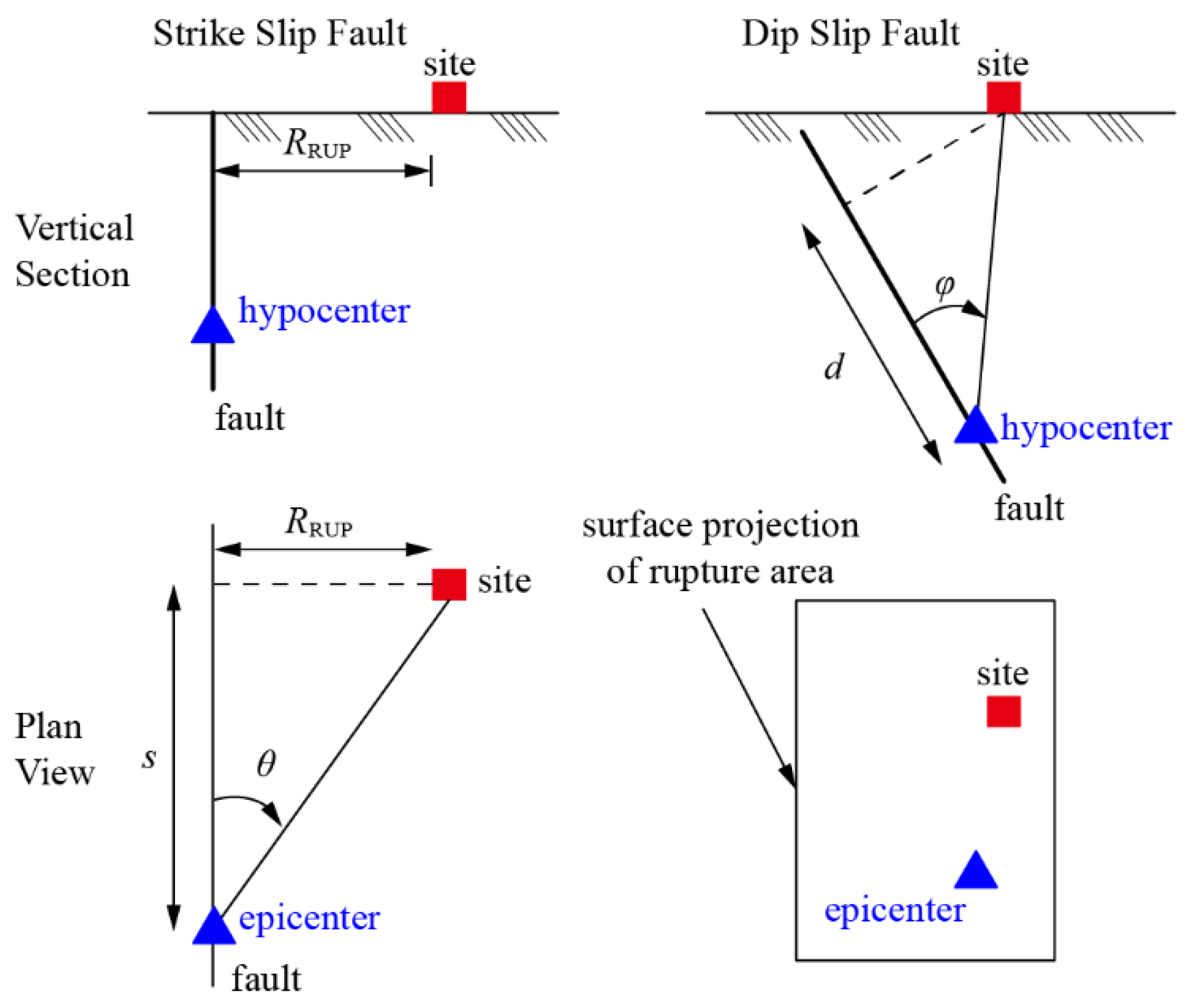
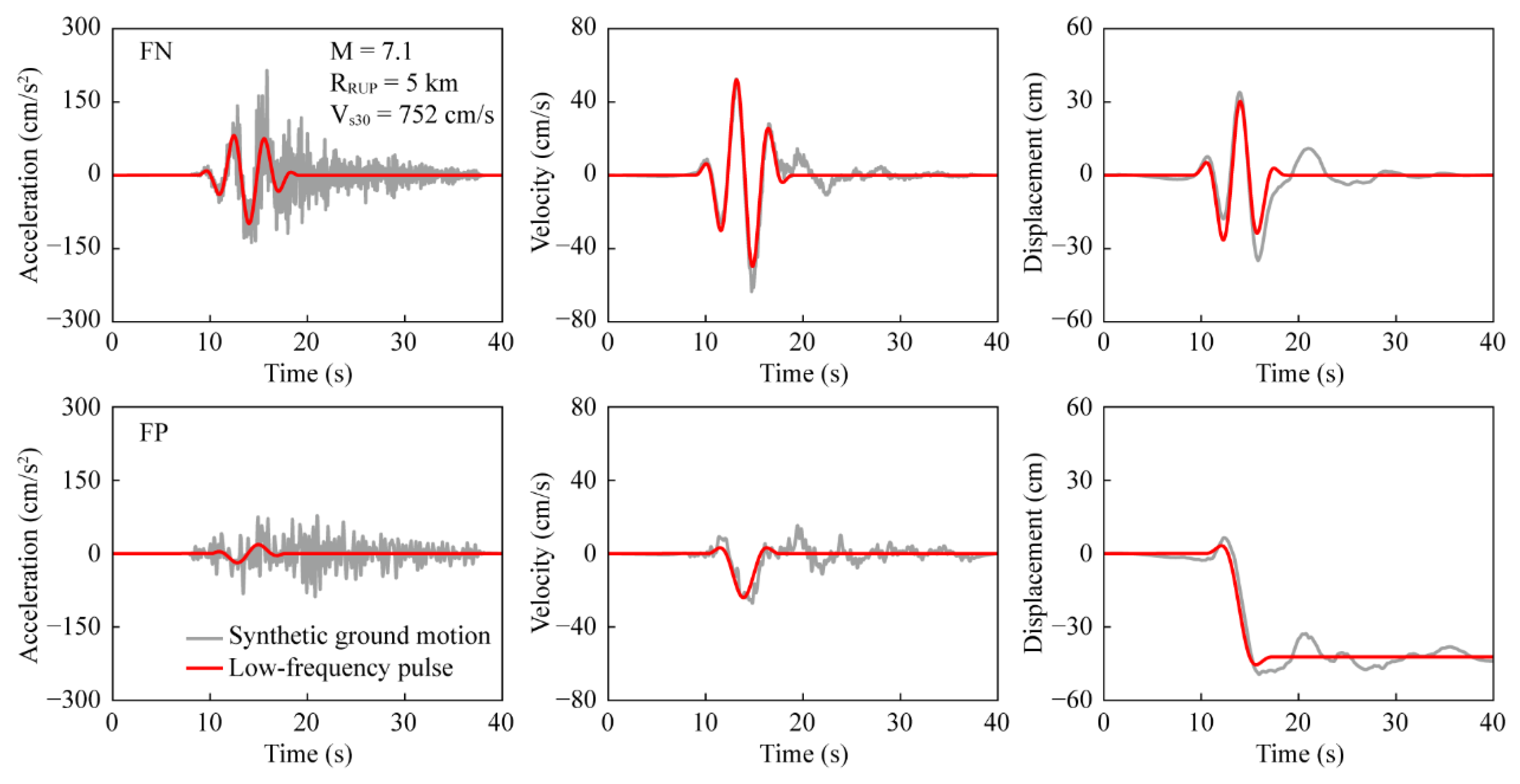
3.1. Ground-Motion Models

Dabaghi et al. [32] pointed out that the residual of a velocity pulse motion after removal of the pulse is generally a broadband time series. A model proposed by Rezaeian et al. [30,31] and adopted by Dabaghi et al. [32,33,34] can be used to describe these broadband motions. The expression of this MFW model is:
a MFW = q ( t ) { 1 σ h ( t ) t h [ t     τ , λ ( τ ) ] w ( τ ) d τ }
where w(t) is a white-noise process, σh(t) is the standard deviation of the process defined by the integral, q(t) is a time-modulating function that characterizes the root-mean-square of the acceleration process, and h[t − τ, λ(τ)] is the unit-impulse response function (IRF) of a linear filter with the time-varying parameter λ(τ) = [wf(τ), ξf(τ)], given as follows:
h [ t τ , λ ( τ ) ] = { ω f ( τ ) 1 ξ f 2 ( τ ) e ξ f ( τ ) ω f ( τ ) ( t τ ) sin [ ω f ( τ ) 1 ξ f 2 ( τ ) ( t τ ) ] , τ     t 0 ,   elsewhere
where τ is the time of the pulse, ξf(τ) is the filter damping that represents the bandwidth of the acceleration process (regarded as a constant), and ωf(τ) is the filter frequency:
ω f ( τ ) = 2 π [ f mid + f ( τ t mid ) ]
where fmid is the filter frequency at the middle of the motion tmid, and f’ is the frequency change rate with time.
For the modulating function q(t), a four-parameter piecewise function is presented as:
q ( t ) = { 0 ,   t     t 0 , q c ( t t 0 , q t max , q t 0 , q ) α , t 0 , q   <   t     t max , q ce [ β ( t t max , q ) ] ,   t max , q   <   t
where t0,q is the starting time, tmax,q is the time that the modulating function arrives at its peak, α is the order of the polynomial at the start of the function, β is the decaying rate of an exponential function in the end phase of the function, and c controls the amplitude of the modulating function. These four parameters (tmax,q, α, β, c) are related to the Arias intensity of the motion.
The model put forward by Mavroeidis et al. [21] (M03 model) has been widely employed for generating the long-period pulse of near-fault motions. Currently, when simulating the fling of the motion, the M03 model is adopted with its original form as follows:
v pul ( t ) = { V p 2 [ 1 + cos ( 2 π γ T p ( t t 0 ) ) ] cos [ 2 π T p ( t t 0 ) + υ ] ,   t 0 γ 2 T p <   t     t 0 + γ 2 T p 0 ,   otherwise
where Vp is the pulse magnitude, Tp is the period, γ is a variable controlling the oscillation number of a pulse, ν is the phase angle, and t0 is the epoch of the peak of the envelope.
For the simulation of the velocity pulse, the form of the MP model proposed by Dabaghi et al. [32] is adopted:
v pul ( t ) = { { V p 2 cos [ 2 π ( t t max , p T p ) + υ ] D r γ T p } { 1 + cos [ 2 π γ ( t t max , p T p ) ] } ,   t max , p γ 2 T p   <   t     t max , p + γ 2 T p   0 ,   elsewhere
where t0 in Equation (8) is replaced by tmax,p, and Dr is a permanent displacement represented with D r = V p T p sin ( ν + γ π ) sin ( ν γ π ) 4 π ( 1 γ 2 ) .
Additionally, the FN component of the simulated motions is checked, adopting the criteria put forward by Baker [46] to ensure that it contains a velocity pulse. The three criteria can be found in [46] and are given here for convenience:
(1)
The equation of the pulse indicator (larger than 0.85) is given as:
Pulse   indicator = 1 1 + e 23.3 + 14.6 ( PGV   ratio ) + 20.5 ( energy   ratio )
where the PGV ratio is defined as the PGV of the residual record divided by the original record’s PGV and the energy ratio with a similar definition.
(2)
The pulse occurs at the early stage of the motion, as indicated by the time when the original record reaches 20% of its total cumulative squared velocity (CSV) and is greater than the time at which the pulse reaches 10% of its CSV.
(3)
The PGV of the motion is larger than 30 cm/s.

3.2. Determination of the Input Parameters of the Models

Input parameters of the models for high-frequency components and the forward-directivity pulse are determined through linear predictive equations developed by Dabaghi et al. [32,33,34], according to the source and site characteristics. Specifically, seven parameters are selected for the predictive equations, including the type of faulting (F), the moment magnitude (M), the depth to the top of the rupture plane (ZTOR), the closest distance from the site to the fault rupture (RRUP), the shear-wave velocity of the top 30 m of soil at the site (Vs30), and directivity parameters s (or d) and θ (or φ). The schematic of the directivity parameters is plotted in Figure 1. Detailed procedures for the regression of these model parameters can be found in [32,33,34].
Input parameters of the fling model are determined following the guidelines recommended by Yang et al. [28]. It is noteworthy that choosing equations for estimating the parameters for the fling model is not unique. In this study, the predictive equations proposed by Abrahamson [48] are selected.
Table 1 lists the predictive equations for estimating the input parameters.

4. Vulnerability Analysis of a Fault-Crossing Bridge

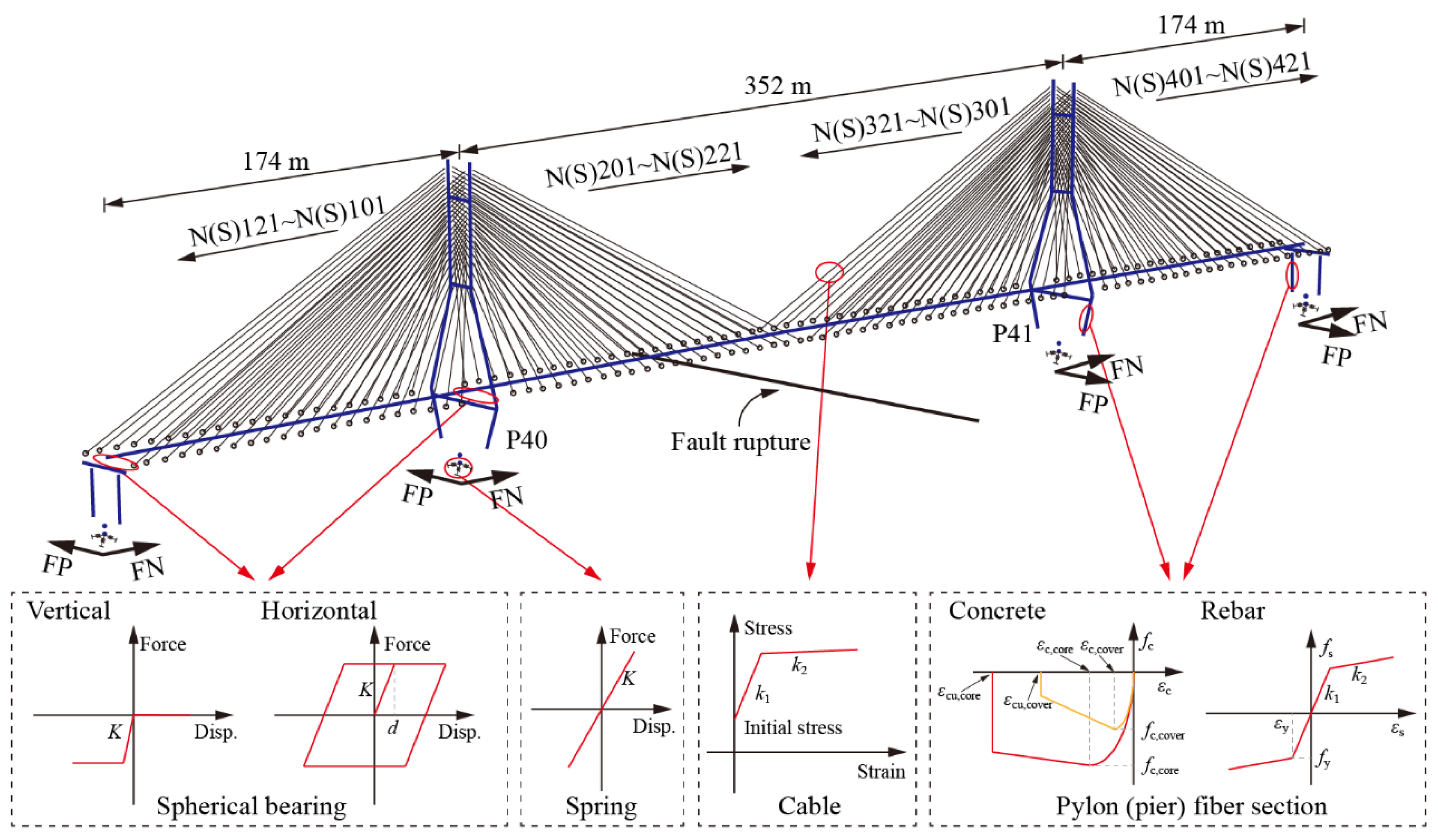
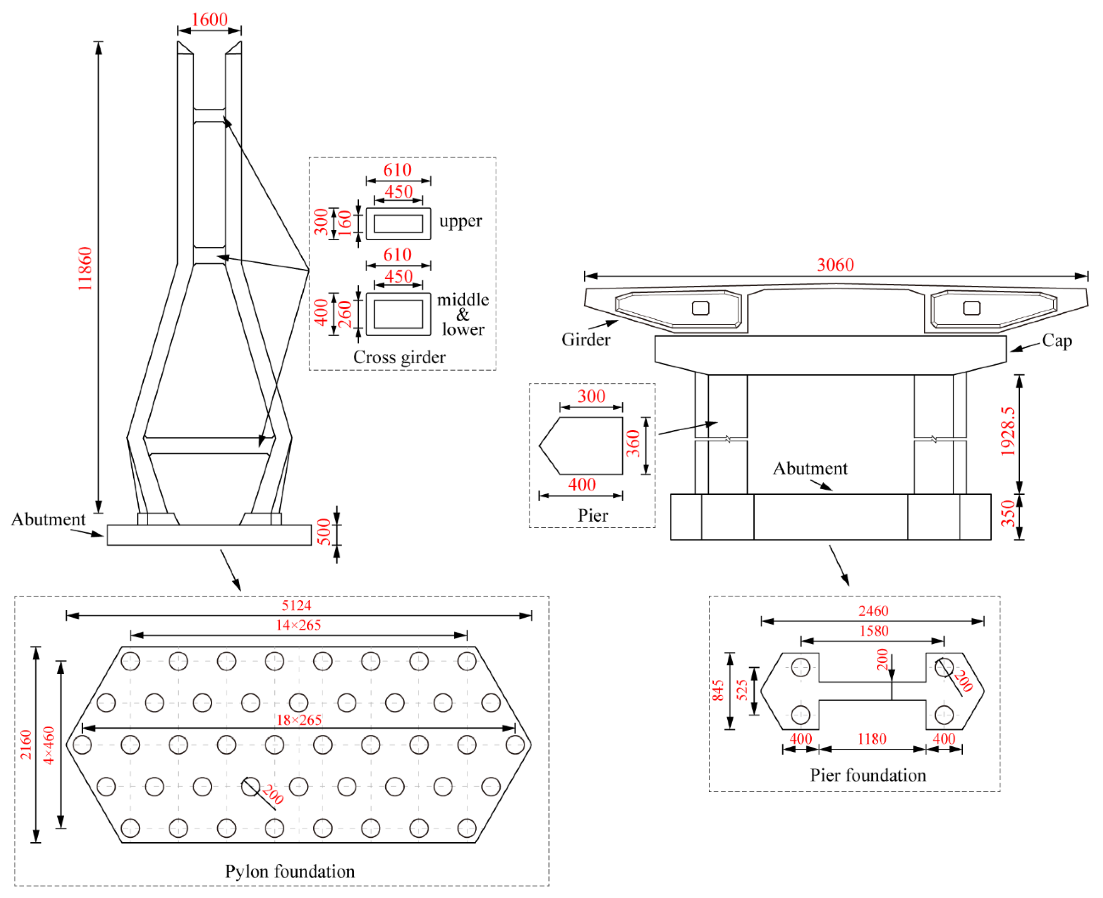
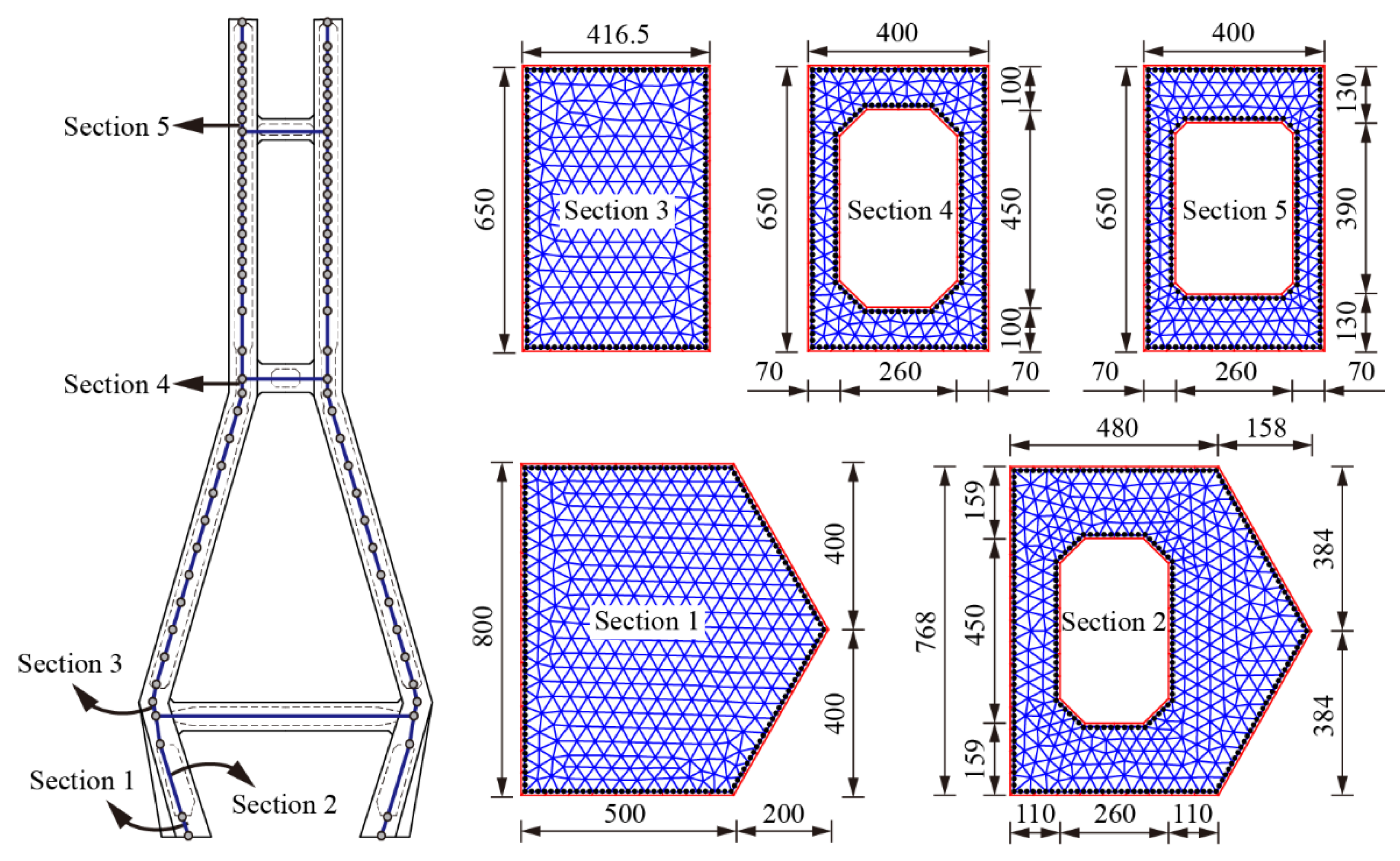
4.1. Depiction of the Analysis Model

A typical cable-stayed bridge is selected as the case study bridge. The bridge has a length of 174 + 352 + 174 m. There are 168 stay cables, whose tensile strength is 1670 MPa, with a fan-typed configuration. The cable force is optimized based on the method proposed by Guo et al. [49].
Wind-resistance bearings are arranged between the girder and pylons in the transverse direction. Note that the dampers, restrainers, and transverse retainers are not considered in this study.
The numerical model of this case bridge is constructed with the OpenSeesPy platform [43], as illustrated in Figure 2. The dimension of the critical components is given in Figure 3. The elastic beam-column element is adopted for the main girder, cap beams, and cross girders, as they are assumed to remain elastic. The plasticity fiber model is used for the sections of pylons and piers. Fiber sections of the tower are presented in Figure 4. The P-delta effect of the pylons is considered. The truss element is used to model the cables. The pile foundation is simulated with three translational and three rotational springs. For the spherical bearing, the no-tension uniaxial material is adopted to simulate the vertical behavior of the bearings. The elastic no-tension material is used to model its axial stiffness for the wind-resistance bearing. The damping ratio of the example bridge is 3%. The first five natural vibration periods of the model are 10.999, 4.537, 3.092, 2.940, and 1.913 s. The first three modes are longitudinal floating vibration, vertical vibration, and transverse floating vibration, respectively.
Material uncertainties are considered for the numerical model of the bridge. In addition, the uncertainty of the actual initial cable forces due to the construction error is also considered. In this study, the compressive strength of the concrete (fc), yield strength of the rebar (fy), initial stiffness of the rebar (E), the ratio between the post-yield and initial stiffness, and the ratio between actual and designed initial cable forces (R) are modeled as random variables. Table 2 summarizes the statistical information of these uncertainty parameters.

4.2. Ground Motions

It is pointed out that the model developed by Dabaghi et al. should be used within the boundaries of the database, which are 6 ≤ M ≤ 7.5, 5 < RRUP ≤ 25 km, and 400 < Vs30 < 1000 m/s [32]. Therefore, 25 ground-motion pairs (in FN and FP directions) are simulated with their input parameters randomly generated within the corresponding ranges. It is worth noting that for strike-slip faults, RRUP, s, and θ are correlated with RRUP = stanθ if a straight line can represent the rupture and if the site is located alongside the rupture, as shown in Figure 1. In the present study, only the case of vertical strike-slip faults with surface rupture is considered, and the site is assumed to be perpendicular to the epicenter. As a result, F, ZTOR, s, and θ are constrained as 0, 0, 0, and 90°, respectively, in the simulation. Models of the low-frequency pulses and high-frequency residuals are programmed in Python language. Figure 5 presents the time histories of one of the synthetic motions. The “forward-directivity” pulse in the FN direction and the “fling-step” pulse in the FP direction can be successfully simulated. The random parameters of the 25 synthetic ground-motion pairs are listed in Table 3.
The synthetic motion pairs are then scaled using a factor ranging from 0.5 to 3 with an increment of 0.5. Thus, 150 ground-motion pairs are generated for the nonlinear time-history analysis. Figure 6 presents the spectra displacement of the input ground motions in FN and FP directions. It shows that the component in the FP direction has larger displacements than that in the FN direction in the long-period range.
According to previous studies, cable-stayed bridges are suggested to cross the fault perpendicularly [15]. Therefore, in this study, the fault rupture should cross the bridge in its middle span with an angle of 90°. The time-history series applies to the bridge supports in the FN and FP directions. Because this study focuses on the vertical strike-slip scenario, the ground dislocation is assumed to distribute equally at the two sides of the fault. As a result, the FN ground motions are the same on each fault side, whereas the FP ground motions have equal amplitudes but with reversed polarity [53] (as shown in Figure 7). To exclude the interference of the effect of vertical ground motions and mainly consider the effect of the FN and FP components, the vertical motions are not considered in this study. The wave passage effect is not considered as well.

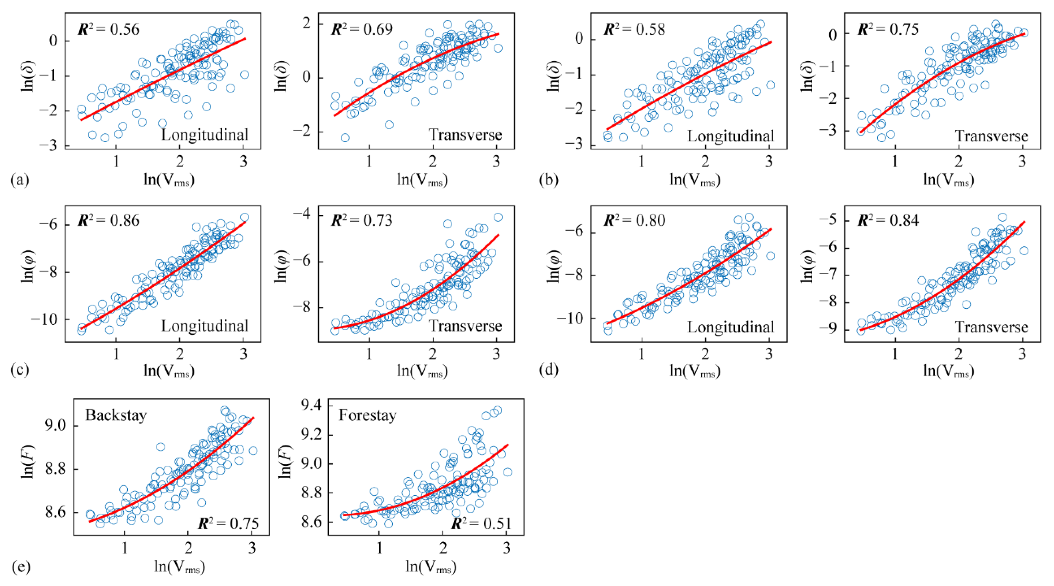
4.3. Optimal IM Determination and PSDMs Establishment

The selection of optimal IMs is essential for establishing reliable PSDMs. In this study, 12 IM candidates are examined to identify the optimal one for the fault-crossing cable-stayed bridge. Table 4 gives the definitions of the studied IMs. The IMs are divided into three groups: acceleration-related, velocity-related, and displacement-related. Note that only structure-independent IMs are used in the current study.
The geometric mean of the IMs for the FN and FP input ground motions is adopted here to represent the IM of a motion pair:
IM = IM FN   ×   IM FP
During the analyses, responses of the following components (engineering demand parameters, EDPs) are recorded: (1) curvature of Section 1, φS1; (2) curvature of Section 3, φS3; (3) bearing displacement between girder and pier σb,pier; (4) bearing displacement between girder and pylon σb,pylon; (5) force of the longest backstay cable (N121) Fbc; and (6) force of the longest forestay cable (N221) Ffc. The upper sides of the pylon are less vulnerable than the lower sides, and the pier has a small effect on the seismic responses of the bridge compared to the pylon [38], so their responses are not considered in this study. Quadratic polynomials are adopted to construct the PSDMs.
Because the regression model is quadratic, the criteria of an optimal IM for linear regressions (practically, efficiency, proficiency, and sufficiency [57]) are not appropriate here. In this study, the determination coefficient (R2) of the regression is used to judge whether an IM is optimal or not. The definition of R2 is given as follows:
R 2 = ( y ^ y ¯ ) 2 ( y y ¯ ) 2 = 1 ( y y ^ ) 2 ( y y ¯ ) 2
where y is the sample value, y ^ is the regression value, and y is the mean of the sample. The larger R2, the better the regression is.
Figure 8 plots the determination coefficients for the regressions in the case of each IM candidate. As shown in Figure 8, the largest R2 varies for different EDPs. Additionally, R2 can be significantly different for an EDP in different directions. For example, PGV performs well in predicting the transverse bearing displacements, pylon responses, and the backstay cable’s force but may not provide reliable predictions on bearing displacements in the longitudinal direction and the force of forestay cables. Therefore, it is difficult to identify the optimal IM from R2 directly. The multicriteria decision-making (MCDM) method is adopted to tackle this issue. In each MCD, there are several alternatives and criteria. The alternative with the highest score is selected as the best one and is placed in the first rank [58]. In this research, different IMs are considered alternatives, and the corresponding determination coefficients R2 for different components are chosen as criteria.
The weights of different components are assigned based on 10-point scale qualitative evaluations, as shown in Table 5. Moreover, the weights of a component in different directions are considered to be the same for simplicity. Compared with the bearings, cables and pylons are considered more critical because their failure would cause bridge collapse. As a result, the weights of pylons and cables are both assigned as 10, whereas the weights of bearings are assigned 3, 5, or 7.
After assigning the weights, a weighted sum method calculates the scores and ranks the IMs. Results of the MCDM method are tabulated in Table 6.
According to the rank of the IMs for different weight assignments, it is found that Vrms is the optimal one among the 12 candidates. Results also demonstrate that the velocity-dependent IMs perform better than the others for all the weight assignments. Moreover, it is worth mentioning that PGA, which has been used as the optimal IM for seismic fragility analyses in previous studies [41,59], is inappropriate for cable-stayed bridges that cross fault ruptures. The PSDMs established for each EDP using Vrms are illustrated in Figure 9, and the corresponding regression coefficients are listed in Table 7. It is worth noting that the hazard curve for Vrms is unavailable. However, it is possible to establish the correlation between Vrms and an IM with available hazard curves, with the development of ground-motion prediction equations, using similar methods introduced in [60].

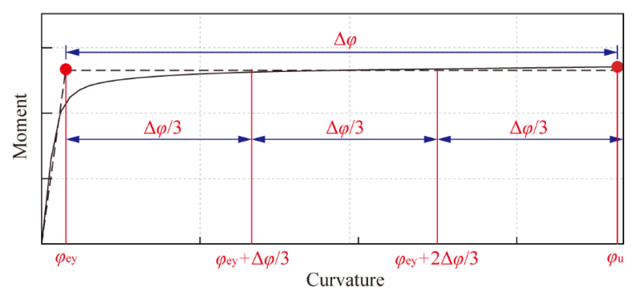
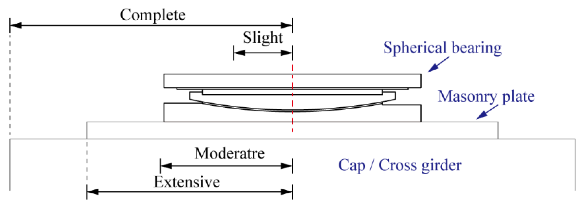
4.4. Definition of the Damage Index

Four limit states are considered, namely slight, moderate, extensive, and complete. For the pylon sections, the value of each damage state proposed by Feng [61] is adopted in this study. Figure 10 illustrates the moment-curvature curve for a pylon section. The slight damage state is characterized by the equivalent yield curvature (φey), whereas the complete one is characterized by the ultimate curvature (φu). Taking the difference between φey and φu as Δφ, the curvatures that represent moderate and extensive damage states are defined as (φey + Δφ/3) and (φey + 2Δφ/3), respectively. For the spherical bearings, the slight limit state is defined to be the maximum allowable bearing displacement under normal service conditions; the distance between the center of the bearing and the edge of the masonry plate is defined as the threshold of the extensive damage state, and the threshold of the moderate damage state is defined as the median of slight and extensive damage states; when the center of the bearing moves over the edge of the substructure (i.e., the cap or cross girder), the bearing is considered to be completely damaged. Figure 11 gives the definition of the damage states for the bearing. For the cable forces, the threshold of the complete damage state is defined as the cable’s breaking force. The difference between the initial and cable-breaking force is quartered, and the quartering points are defined as slight, moderate, and extensive damage thresholds.
Table 8 summarizes the damage index of different damage states for the EDPs, where SC and βC mean the median and logarithmic standard deviation, respectively. Note that the thresholds of slight, moderate, and extensive damage states for the bearings are the same in longitudinal and transverse directions. However, the bearing’s complete damage state threshold is larger in the transverse direction because of the adequate distance between the bearing’s center line and the cap’s transverse edge.

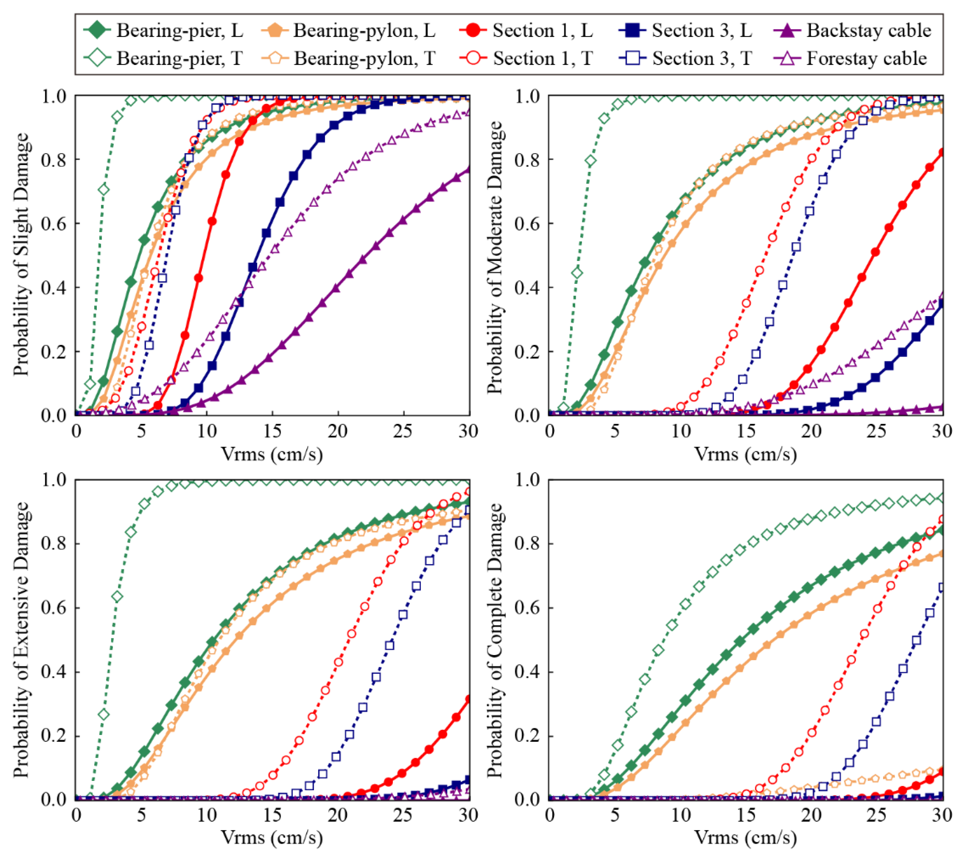
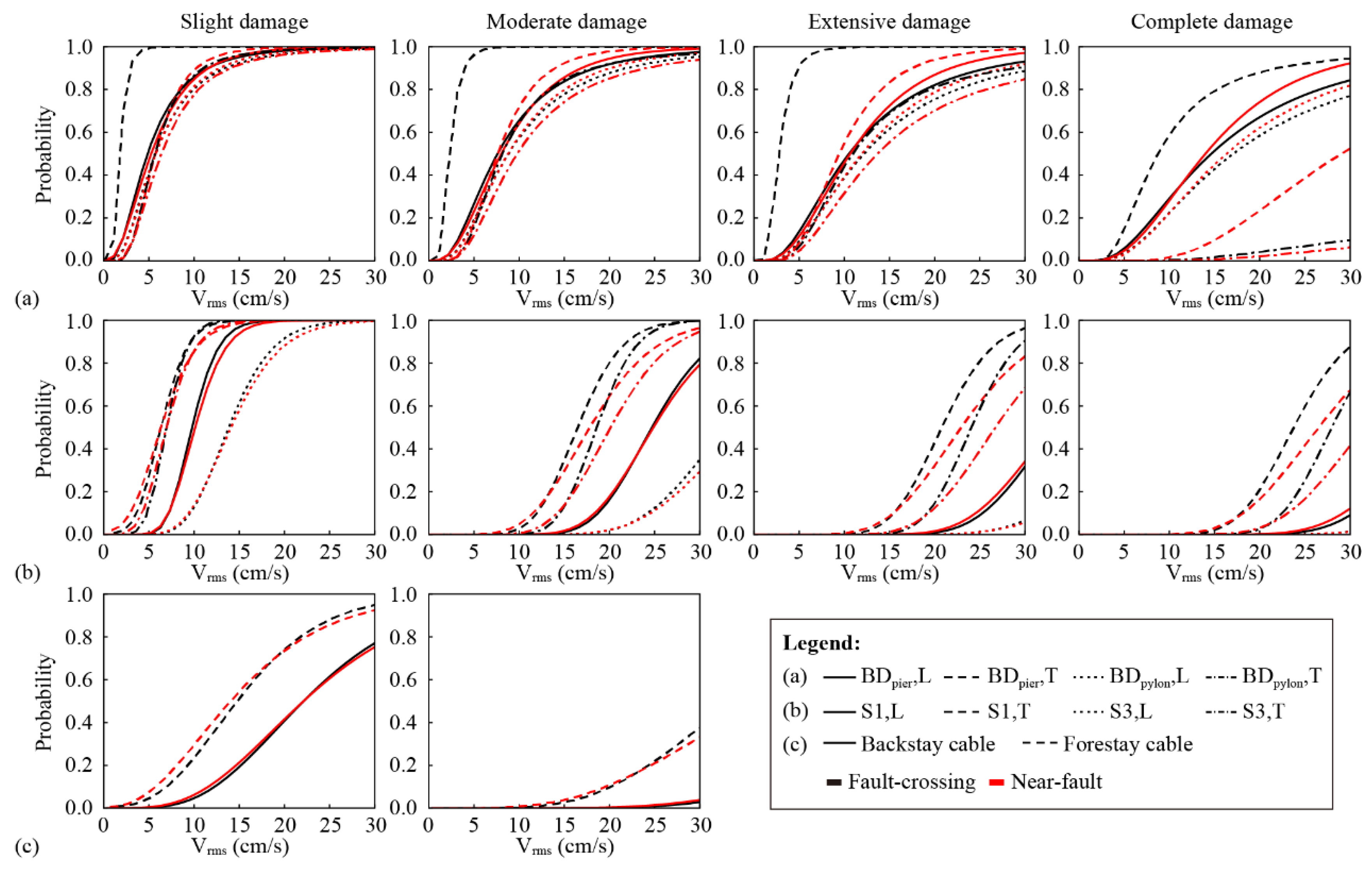
4.5. Component Fragility Curves

Utilizing the aforementioned PSDMs, the component fragility curves for the fault-crossing bridge under different limit states are developed, as presented in Figure 12. As shown in Figure 12, the bearings at girder–pier locations are the most fragile components for all damage states, especially in the transverse direction. Comparing the bearings at different locations, their vulnerabilities are similar in the longitudinal direction but different in the transverse direction. This can be attributed to the rotation of the deck caused by the permanent displacement.
Figure 12 also shows that the pylon sections are more vulnerable in the transverse direction, and the pylon bottom section (Section 1) is more vulnerable than the section of the connection zone between the pylon and lower cross-girder (Section 3). Although the capacity of Section 1 is stronger than that of Section 3 (as shown in Figure 4), the pylon bottom can suffer larger seismic forces under earthquakes, which results in its higher vulnerability.
As for the cables, they are likely to experience only slight and moderate damage. Furthermore, the forestay one appears more vulnerable than the backstay one. This is because the girder’s inertia force is undertaken alone by the forestay cables in the middle span and the backstay cables and transition piers in the side span.

5. Comparison of the Fragility of the Bridge Subjected to Fling-Step and Near-Faults Motions

To investigate the influence of traversing a fault rupture on the vulnerability of cable-stayed bridges, fragility curves of the same case bridge near the fault rupture are developed as a comparison. The finite element model, input ground motions, selected IM, and EDPs are the same as those described in previous sections. The only difference is that the transverse excitations are applied to the bridge with equal amplitudes and the same polarity for the near-fault scenario, as shown in Figure 13.
Figure 14 compares the component fragility curves of the bridge subjected to near-fault and fling-step motions. Fragility curves of the cables under extensive and complete damage states are not plotted because of their low damage-exceedance probabilities. Table 9 presents the median value (the Vrms associated with the 50% exceedance probability) of the fragility curves across the four limit states. Note that a larger median Vrms means the component is less vulnerable.
Figure 14a depicts that the transverse vulnerability of the bearings at the girder–pier location is significantly different for the two scenarios. Bearings at that location are much more vulnerable to fault-crossing cable-stayed bridges due to the deck’s rotation, which is, as mentioned earlier, caused by permanent ground dislocations. As presented in Table 9, the median root-mean-square velocities of the bearings’ longitudinal vulnerabilities are similar for the two case bridges. However, Figure 14a shows that when the intensity of ground motions is high, bearings of the bridge subjected to near-fault motions are a little more vulnerable in the longitudinal direction.
Figure 14b compares the vulnerabilities of the pylons for fault-crossing and near-fault bridges. It illustrates that the pylon’s vulnerabilities for the two scenarios are comparable under the slight damage state. However, the pylon’s transverse vulnerabilities of fault-crossing bridges become higher under the other three damage states, whereas its longitudinal vulnerabilities remain comparable. According to Table 9, the median root-mean-square velocities of the transverse moderate, extensive, and complete damage states of Section 1 for near-fault bridges are 8%, 10%, and 12% larger than those for fault-crossing bridges. Similarly, differences in median values of these damage states of Section 3 between the two cases are 8%, 11%, and 13%, respectively. This is because the transverse seismic responses of the pylon for the fling-step bridge contain not only dynamic ones but also static ones exerted by the ground dislocation. Thus, the transverse seismic demand of the pylon for fault-crossing bridges can be more significant than that for near-fault bridges. In other words, there is a high risk of suffering severe damages in the transverse direction for the pylons if the bridge crosses a fault.
Figure 14c and Table 9 show that the vulnerabilities of the stay cables are almost the same under slight and moderate damage states, whether the bridge is across a fault rupture or not. Such phenomena can be attributed to the fact that the cable force is mainly affected by the vertical and longitudinal deformations of the girder and pylons, and these deformations of the near-fault bridges are supposed to be similar to those of the fault-crossing bridges.

6. Conclusions

This study aims at the seismic fragility assessment for cable-stayed bridges crossing faults. Synthetic fling-step motions are generated and applied to the numerical models. The optimal ground-motion intensity measure for the bridge is identified among 12 candidates. Fragility analysis is conducted, and the results are compared. The conclusions are summarized as follows:
(1)
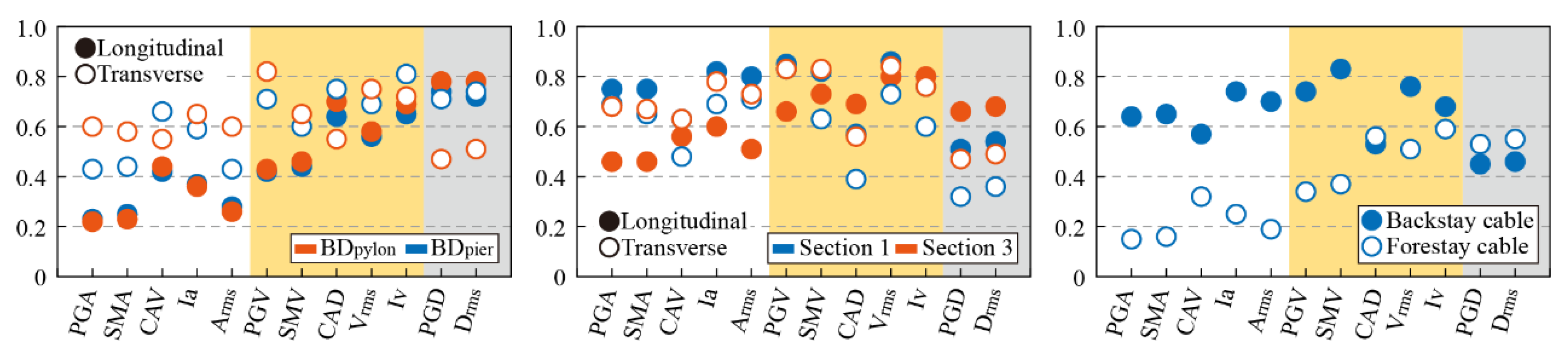
According to the coefficient of determination R2 and the multicriteria decision-making (MCDM) method, the root-mean-square velocity (Vrms) is identified as the optimal IM for the cable-stayed bridge crossing faults.
(2)
Bearings are the most fragile components for the fault-crossing bridge, especially in the transverse direction of those on transition piers. The pylon bottom is more vulnerable than the connection zone between the pylon and cross-girder. In contrast, the cables are not likely to suffer severe damage.
(3)
Compared with the bridge subjected to near-fault motions, the vulnerability of pylons and bearings of the fault-crossing bridge becomes higher in the transverse direction. However, the vulnerability of the cables is comparable.
(4)
This study limits the fragility analysis of cable-stayed bridges subjected to vertical strike-slip faults with a fault crossing angle of 90°. The vulnerability of cable-stayed bridges crossing dip-slip and oblique-slip faults or existing bridges with other fault crossing angles needs further investigation.

Author Contributions

Conceptualization, J.G., Y.G., W.W., S.C. and X.D.; methodology, J.G., Y.G.; investigation, W.W. and X.D.; writing—original draft preparation, J.G. and Y.G.; writing—review and editing, S.C. and X.D.; supervision, X.D.; formal analysis, J.G. and Y.G.; validation, W.W. and X.D. All authors have read and agreed to the published version of the manuscript.

Funding

This research was funded by the National Key Research and Development Program of China (2019YFE0112300); The Shanghai Post-doctoral Excellent Program (2021333); The Post-doctoral Innovation Practice Base Program of Shanghai Yangpu District; and the National Natural Science Foundation of China (51978512).

Conflicts of Interest

The authors declare no conflict of interest.

References

  1. Hui, Y.; Wang, K.; Wu, G.; Li, C. Seismic responses of bridges crossing faults and their best crossing angles. J. Vib. Shock 2015, 34, 6–11. (In Chinese) [Google Scholar]
  2. Yang, S.; Mavroeidis, G.P. Bridges crossing fault rupture zones: A review. Soil Dyn. Earthq. Eng. 2018, 113, 545–571. [Google Scholar] [CrossRef]
  3. Yang, S.; Mavroeidis, G.P.; Tsopelas, P. Seismic response study of ordinary and isolated bridges crossing strike-slip fault rupture zones. Earthq. Eng. Struct. Dyn. 2021, 50, 2841–2862. [Google Scholar] [CrossRef]
  4. Park, S.W.; Ghasemi, H.; Shen, J.; Somerville, P.G.; Yen, W.P.; Yashinsky, M. Simulation of the seismic performance of the Bolu Viaduct subjected to near-fault ground motions. Earthq. Eng. Struct. Dyn. 2004, 33, 1249–1270. [Google Scholar] [CrossRef]
  5. Goel, R.K.; Asce, F.; Chopra, A.K.; Asce, M. Role of Shear Keys in Seismic Behavior of Bridges Crossing Fault-Rupture Zones. J. Bridg. Eng. 2008, 13, 398–408. [Google Scholar] [CrossRef] [Green Version]
  6. Goel, R.K.; Chopra, A.K. Nonlinear analysis of ordinary bridges crossing fault-rupture zones. J. Bridg. Eng. 2009, 14, 216–224. [Google Scholar] [CrossRef] [Green Version]
  7. Goel, R.K.; Chopra, A.K. Linear analysis of ordinary bridges crossing fault-rupture zones. J. Bridg. Eng. 2009, 14, 203–215. [Google Scholar] [CrossRef] [Green Version]
  8. Ucak, A.; Mavroeidis, G.P.; Tsopelas, P. Assessment of Fault Crossing Effects on a Seismically Isolated Multi-Span Bridge. In Proceedings of the 15th World Conference on Earthquake Engineering (15WCEE), Lisbon, Portugal, 24–28 September 2012. [Google Scholar]
  9. Ucak, A.; Mavroeidis, G.P.; Tsopelas, P. Behavior of a seismically isolated bridge crossing a fault rupture zone. Soil Dyn. Earthq. Eng. 2014, 57, 164–178. [Google Scholar] [CrossRef]
  10. Yang, H.; Li, J. Response analysis of seismic isolated bridge under influence of fault-crossing ground motions. J. Tongji Univ. (Nat. Sci.) 2015, 43, 1144–1152. (In Chinese) [Google Scholar] [CrossRef]
  11. Zhang, F.; Li, S.; Wang, J.; Zhang, J. Effects of fault rupture on seismic responses of fault-crossing simply-supported highway bridges. Eng. Struct. 2020, 206, 110104. [Google Scholar] [CrossRef]
  12. Sharabash, A.M.; Andrawes, B.O. Application of shape memory alloy dampers in the seismic control of cable-stayed bridges. Eng. Struct. 2009, 31, 607–616. [Google Scholar] [CrossRef]
  13. Zhong, J.; Jeon, J.-S.; Yuan, W.; DesRoches, R. Impact of Spatial Variability Parameters on Seismic Fragilities of a Cable-Stayed Bridge Subjected to Differential Support Motions. J. Bridg. Eng. 2017, 22, 04017013. [Google Scholar] [CrossRef]
  14. Zeng, C.; Song, G.; Jiang, H.; Huang, L.; Guo, H.; Ma, X. Nonliear Seismic Response Characteristics of Fault-crossing Single-tower Cable-stayed Bridge. China J. Highw. Transp. 2021, 34, 230–245. (In Chinese) [Google Scholar]
  15. Gu, Y.; Guo, J.; Dang, X.; Yuan, W. Seismic performance of a cable-stayed bridge crossing strike-slip faults. Structures 2022, 35, 289–302. [Google Scholar] [CrossRef]
  16. Wu, Y.M.; Wu, C.F. Approximate recovery of coseismic deformation from Taiwan strong-motion records. J. Seismol. 2007, 11, 159–170. [Google Scholar] [CrossRef]
  17. Iwan, W.D.; Moser, M.A.; Peng, C.-Y. Some observations on strong-motion earthquake measurement using a digital accelerograph. Bull. Seismol. Soc. Am. 1985, 75, 1225–1246. [Google Scholar] [CrossRef]
  18. Boore, D.M. Effect of baseline corrections on displacements and response spectra for several recordings of the 1999 Chi-Chi, Taiwan, earthquake. Bull. Seismol. Soc. Am. 2001, 91, 1199–1211. [Google Scholar] [CrossRef] [Green Version]
  19. Lin, Y.; Zong, Z.; Tian, S.; Lin, J. A new baseline correction method for near-fault strong-motion records based on the target final displacement. Soil Dyn. Earthq. Eng. 2018, 114, 27–37. [Google Scholar] [CrossRef]
  20. Charles, M. An Analytical Model for Near-Fault Ground Motions and the Response of SDOF Systems. In Proceedings of the 7th U.S. National Conference on Earthquake Engineering, Boston, MA, USA, 21–25 July 2002. [Google Scholar]
  21. Mavroeidis, G.P.; Papageorgiou, A.S. A mathematical representation of near-fault ground motions. Bull. Seismol. Soc. Am. 2003, 93, 1099–1131. [Google Scholar] [CrossRef]
  22. Makris, N.; Black, C.J. Dimensional Analysis of Rigid-Plastic and Elastoplastic Structures under Pulse-Type Excitations. J. Eng. Mech. 2004, 130, 1006–1018. [Google Scholar] [CrossRef]
  23. Hoseini Vaez, S.R.; Sharbatdar, M.K.; Ghodrati Amiri, G.; Naderpour, H.; Kheyroddin, A. Dominant pulse simulation of near fault ground motions. Earthq. Eng. Eng. Vib. 2013, 12, 267–278. [Google Scholar] [CrossRef]
  24. Kamai, R.; Abrahamson, N.; Graves, R. Adding fling effects to processed ground-motion time histories. Bull. Seismol. Soc. Am. 2014, 104, 1914–1929. [Google Scholar] [CrossRef]
  25. Burks, L.S.; Baker, J.W. A predictive model for fling-step in near-fault ground motions based on recordings and simulations. Soil Dyn. Earthq. Eng. 2016, 80, 119–126. [Google Scholar] [CrossRef]
  26. Yadav, K.K.; Gupta, V.K. Near-fault fling-step ground motions: Characteristics and simulation. Soil Dyn. Earthq. Eng. 2017, 101, 90–104. [Google Scholar] [CrossRef]
  27. Hamidi, H.; Khosravi, H.; Soleimani, R. Fling-step ground motions simulation using theoretical-based Green’s function technique for structural analysis. Soil Dyn. Earthq. Eng. 2018, 115, 232–245. [Google Scholar] [CrossRef]
  28. Yang, S.; Mavroeidis, G.P.; Ucak, A. Analysis of bridge structures crossing strike-slip fault rupture zones: A simple method for generating across-fault seismic ground motions. Earthq. Eng. Struct. Dyn. 2020, 49, 1281–1307. [Google Scholar] [CrossRef]
  29. Papageorgiou, A.S.; Aki, K. A specific barrier model for the quantitative description of inhomogenous faulting and the prediction of strong ground motion. Bull. Seismol. Soc. Am. 1983, 73, 693–722. [Google Scholar] [CrossRef]
  30. Rezaeian, S.; Kiureghian, A. Der A stochastic ground motion model with separable temporal and spectral nonstationarities. Earthq. Eng. Struct. Dyn. 2008, 37, 1565–1584. [Google Scholar] [CrossRef]
  31. Rezaeian, S.; Kiureghian, A. Der Simulation of synthetic ground motions for specified earthquake and site characteristics. Earthq. Eng. Struct. Dyn. 2010, 39, 1155–1180. [Google Scholar] [CrossRef]
  32. Dabaghi, M.; Der Kiureghian, A. Stochastic Modeling and Simulation of Near-Fault Ground Motions for Performance-Based Earthquake Engineering; University of California: Berkeley, CA, USA, 2014. [Google Scholar]
  33. Dabaghi, M.; Der Kiureghian, A. Stochastic model for simulation of near-fault ground motions. Earthq. Eng. Struct. Dyn. 2016, 46, 963–984. [Google Scholar] [CrossRef]
  34. Dabaghi, M.; Der Kiureghian, A. Simulation of orthogonal horizontal components of near-fault ground motion for specified earthquake source and site characteristics. Earthq. Eng. Struct. Dyn. 2018, 47, 1369–1393. [Google Scholar] [CrossRef]
  35. Pang, Y.; Wu, X.; Shen, G.; Yuan, W. Seismic Fragility Analysis of Cable-Stayed Bridges Considering Different Sources of Uncertainties. J. Bridg. Eng. 2014, 19, 04013015. [Google Scholar] [CrossRef]
  36. Zhong, J.; Pang, Y.; Jeon, J.S.; Desroches, R.; Yuan, W. Seismic fragility assessment of long-span cable-stayed bridges in China. Adv. Struct. Eng. 2016, 19, 1797–1812. [Google Scholar] [CrossRef]
  37. Zhong, J.; Jeon, J.S.; Ren, W.X. Risk assessment for a long-span cable-stayed bridge subjected to multiple support excitations. Eng. Struct. 2018, 176, 220–230. [Google Scholar] [CrossRef]
  38. Zhong, J.; Jeon, J.-S.; Shao, Y.-H.; Chen, L. Optimal Intensity Measures in Probabilistic Seismic Demand Models of Cable-Stayed Bridges Subjected to Pulse-Like Ground Motions. J. Bridg. Eng. 2019, 24, 04018118. [Google Scholar] [CrossRef]
  39. Wu, W.; Li, L.; Shao, X. Seismic Assessment of Medium-Span Concrete Cable-Stayed Bridges Using the Component and System Fragility Functions. J. Bridg. Eng. 2016, 21, 04016027. [Google Scholar] [CrossRef]
  40. Wang, J.; Li, S.; Zhang, F. Seismic fragility analyses of long-span cable-stayed bridge isolated by SMA Wire-based Smart Rubber Bearing in near-fault regions. China J. Highw. Transp. 2017, 30, 30–39. (In Chinese) [Google Scholar] [CrossRef]
  41. Li, C.; Li, H.N.; Hao, H.; Bi, K.; Chen, B. Seismic fragility analyses of sea-crossing cable-stayed bridges subjected to multi-support ground motions on offshore sites. Eng. Struct. 2018, 165, 441–456. [Google Scholar] [CrossRef]
  42. Wei, B.; Hu, Z.; He, X.; Jiang, L. Evaluation of optimal ground motion intensity measures and seismic fragility analysis of a multi-pylon cable-stayed bridge with super-high piers in Mountainous Areas. Soil Dyn. Earthq. Eng. 2020, 129, 105945. [Google Scholar] [CrossRef]
  43. Zhu, M.; McKenna, F.; Scott, M.H. OpenSeesPy: Python library for the OpenSees finite element framework. SoftwareX 2018, 7, 6–11. [Google Scholar] [CrossRef]
  44. Mangalathu, S.; Jeon, J.-S.; Padgett, J.E.; DesRoches, R. Performance-based grouping methods of bridge classes for regional seismic risk assessment: Application of ANOVA, ANCOVA, and non-parametric approaches. Earthq. Eng. Struct. Dyn. 2017, 46, 2587–2602. [Google Scholar] [CrossRef]
  45. Pan, Y.; Agrawal, A.K.; Ghosn, M. Seismic Fragility of Continuous Steel Highway Bridges in New York State. J. Bridg. Eng. 2007, 12, 689–699. [Google Scholar] [CrossRef]
  46. Baker, J.W. Quantitative classification of near-fault ground motions using wavelet analysis. Bull. Seismol. Soc. Am. 2007, 97, 1486–1501. [Google Scholar] [CrossRef]
  47. Somerville, P.G.; Smith, N.F.; Graves, R.W.; Abrahamson, N.A. Modification of empirical strong ground motion attenuation relations to include the amplitude and duration effects of rupture directivity. Seismol. Res. Lett. 1997, 68, 199–222. [Google Scholar] [CrossRef]
  48. Abrahamson, N. Velocity pulses in near-fault ground motions. In Proceedings of the UC Berkeley—CUREE Symposium in Honor of Ray Clough and Joseph Penzien, Berkeley, CA, USA, 9–11 May 2002; pp. 40–41. [Google Scholar]
  49. Guo, J.; Yuan, W.; Dang, X.; Alam, M.S. Cable force optimization of a curved cable-stayed bridge with combined simulated annealing method and cubic B-Spline interpolation curves. Eng. Struct. 2019, 201, 109813. [Google Scholar] [CrossRef]
  50. Stefanidou, S.P.; Kappos, A.J. Methodology for the development of bridge-specific fragility curves. Earthq. Eng. Struct. Dyn. 2017, 46, 73–93. [Google Scholar] [CrossRef]
  51. Nielson, B.G.; DesRoches, R. Analytical seismic fragility curves for typical bridges in the central and southeastern United States. Earthq. Spectra 2007, 23, 615–633. [Google Scholar] [CrossRef]
  52. Wang, X.; Shafieezadeh, A.; Ye, A. Optimal intensity measures for probabilistic seismic demand modeling of extended pile-shaft-supported bridges in liquefied and laterally spreading ground. Bull. Earthq. Eng. 2018, 16, 229–257. [Google Scholar] [CrossRef]
  53. Dreger, D.; Hurtado, G.; Chopra, A.; Larsen, S. Near-Fault Seismic Ground Motions; Report No. UCB/EERC-2007/03; Earthquake Engineering Research Center, University of California: Berkeley, CA, USA, 2007. [Google Scholar]
  54. Nuttli, O.W. The Relation of Sustained Maximum Acceleration and Velocity to Earthquake Intensity and Magnitude; Report No. S-73-1; U.S. Army Engineer Waterways Experiment Station: Vicksburg, MI, USA, 1979. [Google Scholar]
  55. Reed, J.W.; Kassawara, R.P. A criterion for determining exceedance of the operating basis earthquake. Nucl. Eng. Des. 1990, 123, 387–396. [Google Scholar] [CrossRef] [Green Version]
  56. Arias, A. A Measure of Earthquake Intensity; MIT Press: Cambridge, MA, USA, 1969. [Google Scholar]
  57. Padgett, J.E.; Nielson, B.G.; Desroches, R. Selection of optimal intensity measures in probabilistic seismic demand models of highway bridge portfolios. Earthq. Eng. Struct. Dyn. 2008, 37, 711–725. [Google Scholar] [CrossRef]
  58. Hedayati Dezfuli, F.; Alam, M.S. Multi-criteria optimization and seismic performance assessment of carbon FRP-based elastomeric isolator. Eng. Struct. 2013, 49, 525–540. [Google Scholar] [CrossRef]
  59. Zhang, C.; Lu, J.; Zhou, Z.; Yan, X.; Xu, L.; Lin, J. Lateral seismic fragility assessment of cable-stayed bridge with diamond-shaped concrete pylons. Shock Vib. 2021, 2021, 2847603. [Google Scholar] [CrossRef]
  60. Bradley, B.A. Empirical correlations between cumulative absolute velocity and amplitude-based ground motion intensity measures. Earthq. Spectra 2012, 28, 37–54. [Google Scholar] [CrossRef] [Green Version]
  61. Feng, R.; Yuan, W.; Sextos, A. Probabilistic loss assessment of curved bridges considering the effect of ground motion directionality. Earthq. Eng. Struct. Dyn. 2021, 50, 3623–3645. [Google Scholar] [CrossRef]
Figure 1. Directivity parameters [47].
Buildings 12 01045 g001
Figure 2. Configuration of the case study bridge.
Buildings 12 01045 g002
Figure 3. Dimension of the bridge components (unit: cm).
Buildings 12 01045 g003
Figure 4. Fiber sections of the pylon (unit: cm).
Buildings 12 01045 g004
Figure 5. Time histories of a synthetic ground-motion pair.
Buildings 12 01045 g005
Figure 6. Response spectra of the 150 ground motions.
Buildings 12 01045 g006
Figure 7. Input ground motions for cable-stayed bridges crossing faults.
Buildings 12 01045 g007
Figure 8. Determination coefficients for the regressions of various EDPs. The background colors denote the type of the IMs (white: acceleration-related; yellow: velocity-related; gray: displacement-related).
Buildings 12 01045 g008
Figure 9. PSDMs for different components: (a) bearing at girder–pier location; (b) bearing at girder–pylon location; (c) Section 1 of the pylon; (d) Section 3 of the pylon; and (e) cables.
Buildings 12 01045 g009
Figure 10. Limit states for the pylons.
Buildings 12 01045 g010
Figure 11. Definition of the damage states for bearings.
Buildings 12 01045 g011
Figure 12. Component fragility curves for the fault-crossing bridge.
Buildings 12 01045 g012
Figure 13. Input ground motions for near-fault cable-stayed bridges.
Buildings 12 01045 g013
Figure 14. Comparison between the component fragility curves of fault-crossing and near-fault cable-stayed bridges for (a) bearings, (b) pylons, and (c) cables.
Buildings 12 01045 g014
Table 1. Predictive equations for the input parameters.
ModelPredictive EquationReference
MFW modelα, β, c, tmax,q, fmid, f’ = F(F, M, ZTOR, RRUP, Vs30, s, θ)
t0,q = 0
[32,33,34]
Directivity pulse modelVp, Tp, γ, ν, tmax,p = F(F, M, ZTOR, RRUP, Vs30, s, θ)[32,33,34]
Fling modelVp = 2Dsite/[Tp/(2 + ε)], ε ∈ (0,0.1]
log(Tp) = log(2 + ε) − 3.00 + 0.50M, ε ∈ (0,0.1]
log(Dsite)avg = −1.70 + 0.50M, (Dsite)max ≈ (Dsite)avg/λ, λ ∈ [0.2,0.8]
γ = 1 + ε, ε ∈ (0,0.1]
ν ≈ 0 or π
t0γTp/2
[28]
(Dsite)max is used to estimate Vp.
Table 2. Uncertainty parameters of the bridge and their probability distribution.
VariableDistribution *Reference
fc,pylonNormal (C50, μ = 32.35 MPa, cov = 0.18)[50]
fc,pierNormal (C40, μ = 26.75 MPa, cov = 0.18)[50]
fyLognormal (HRB400, μ = 400 MPa, cov = 0.08)[51]
ELognormal (μ = 2 × 10⁸ MPa, cov = 0.033)[52]
bLognormal (μ = 0.005, cov = 0.2)[35,52]
RUniform (μ = 1, σ = 0.1)/
* μ denotes the mean; cov denotes the coefficient of variation; σ denotes the standard deviation.
Table 3. Input parameters of the synthetic ground motions.
GMMRRUP (km)Vs30 (m/s)GMMRRUP (km)Vs30 (m/s)
1610702147.35.1873
2718.9446157.26.5508
37.15752167.28.2524
46.715.16421777.9691
57.37.8993186.79651
67.15.8954197.523.4445
76.314.269120615.9588
86.98.2846216.710.8630
97.120.3882227.18.2675
106.17542236.314.3947
117.37.2622246.95.8455
126.212.4905256.915.1587
136.85.9903
F = 0 for strike-slip faults; ZTOR = 0; s = 0; θ = 90°.
Table 4. Description of the considered IMs.
TypeIMDefinitionReference
Acceleration-relatedPGAPeak ground acceleration
Max | a ( t ) | , a(t) is the acceleration time history
/
SMASustained maximum acceleration
third largest peak in a(t)
[54]
CAVCumulative absolute velocity
0 t tot | a ( t ) | dt , ttot is the total duration
[55]
IaArias intensity
π 2 g 0 t tot a 2 ( t ) dt ,
[56]
ArmsRoot-mean-square of acceleration
1 t tot 0 t tot a 2 ( t ) dt
/
Velocity-relatedPGVPeak ground velocity
Max | v ( t ) | , v(t) is the velocity–time history
/
SMVSustained maximum acceleration
third largest peak in v(t)
[54]
CADCumulative absolute displacement
0 t tot | v ( t ) | dt , ttot is the total duration
[55]
VrmsRoot-mean-square of velocity
1 t tot 0 t tot v 2 ( t ) dt
/
IvVelocity intensity
π 2 g 0 t tot v 2 ( t ) dt
[57]
Displacement-relatedPGDPeak ground displacement
Max | d ( t ) | , d(t) is the displacement–time history
/
DrmsRoot-mean-square of displacement
1 t tot 0 t tot d 2 ( t ) dt
/
Table 5. Assignment of values for a 10-point scale [58].
Attribute EvaluationValue
Extremely unimportant0
Very unimportant1
Unimportant3
Average5
Important7
Very important9
Extremely important10
Table 6. Results of the MCDM method.
Weight of CriteriaRank of the Optimal IMs
PylonsCablesBearings1st2nd3rd
10107VrmsIvPGV
10105VrmsIvPGV
10103VrmsIvPGV
Table 7. Regression coefficients for the PSDMs.
EDPLongitudinalEDPTransverseEDP/
abcabcabc
σb,pier−0.0220.979−2.696σb,pier−0.1961.864−2.202Fbc0.0350.0658.522
σb,pylon−0.0591.165−3.054σb,pylon−0.2031.883−3.856Ffc0.065−0.0388.652
φS10.0991.408−11.050φS10.471−0.058−8.963
φS30.1831.091−10.791φS30.3260.408−9.252
Formulation for the quadratic regression: ln(SD) = aln2(IM) + bln(IM) + c.
Table 8. Damage index for different damage states.
EDPSlightModerateExtensiveComplete
SCβCSCβCSCβCSCβC
φS1, longitudinal10.046.10.0511.20.0516.30.06
φS1, transverse10.047.60.0414.30.0420.90.04
φS3, longitudinal10.156.70.0612.50.0618.20.06
φS3, transverse10.137.10.0413.20.0419.30.04
σb, longitudinal (mm)3000.354500.356000.358000.35
σb, transverse (mm)3000.354500.356000.3525000.35
Fbc (kN)85860.1011,7850.1014,9870.1018,1880.10
Ffc (kN)82790.1011,1960.1014,1140.1017,0310.10
βC for bearing displacements and cable forces refers to [13].
Table 9. Median Vrms across different damage states for fault-crossing and near-fault bridges (unit: cm/s).
EDPSlightModerateExtensiveComplete
FCNFFCNFFCNFFCNF
σb,pier, longitudial4.865.247.628.0010.5610.6314.7113.95
σb,pier, transverse1.775.702.287.632.769.438.7329.02
σb,pylon, longitudial5.715.758.818.7612.1711.9017.0816.27
σb,pylon, transverse5.656.378.159.7610.9713.62//
φS1, longitudial9.7710.1224.6724.8833.0832.9339.4938.97
φS1, transverse6.346.3316.4517.8020.7622.9123.7226.49
φS3, longitudial13.8514.1232.8234.6442.3545.3049.3153.18
φS3, transverse6.966.9618.6120.1324.1026.7528.0031.57
Fbc22.0421.7359.9559.08////
Ffc14.8014.0233.7636.57////
Publisher’s Note: MDPI stays neutral with regard to jurisdictional claims in published maps and institutional affiliations.

