
A Bayesian Approach towards Modelling the Interrelationships of Pavement Deterioration Factors


Abstract
:1. Introduction
2. Literature Review: Applications of Bayesian Belief Networks in Pavement Studies
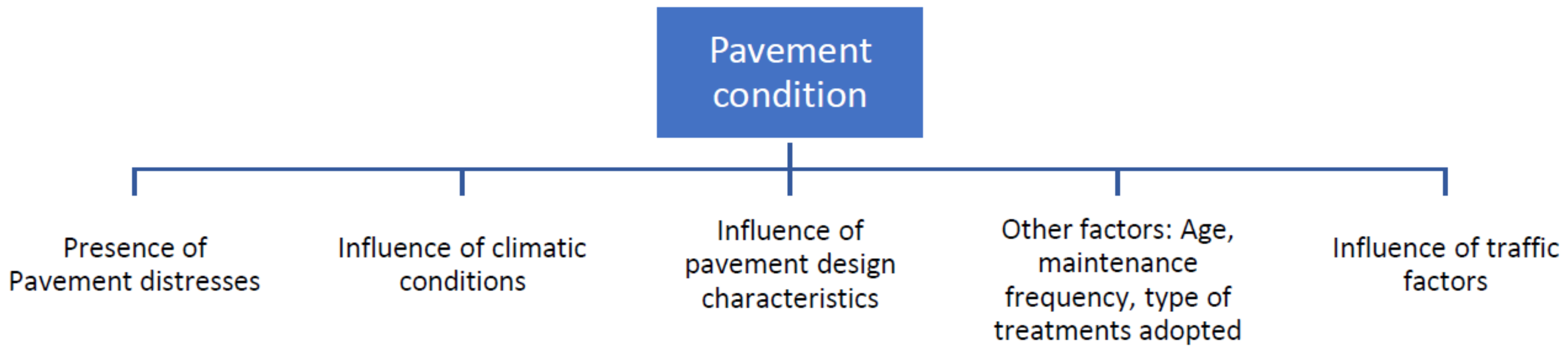
- Estimate the correlations between the road distress parameters: cracking, deflection, IRI and rutting;
- Investigate the influence of external factors related to traffic, environment, and road characteristics on pavement conditions;
- Perform a sensitivity analysis of road distress parameters to understand what type of road distress is prominent on each type of road (arterial, collector, freeway and expressway).
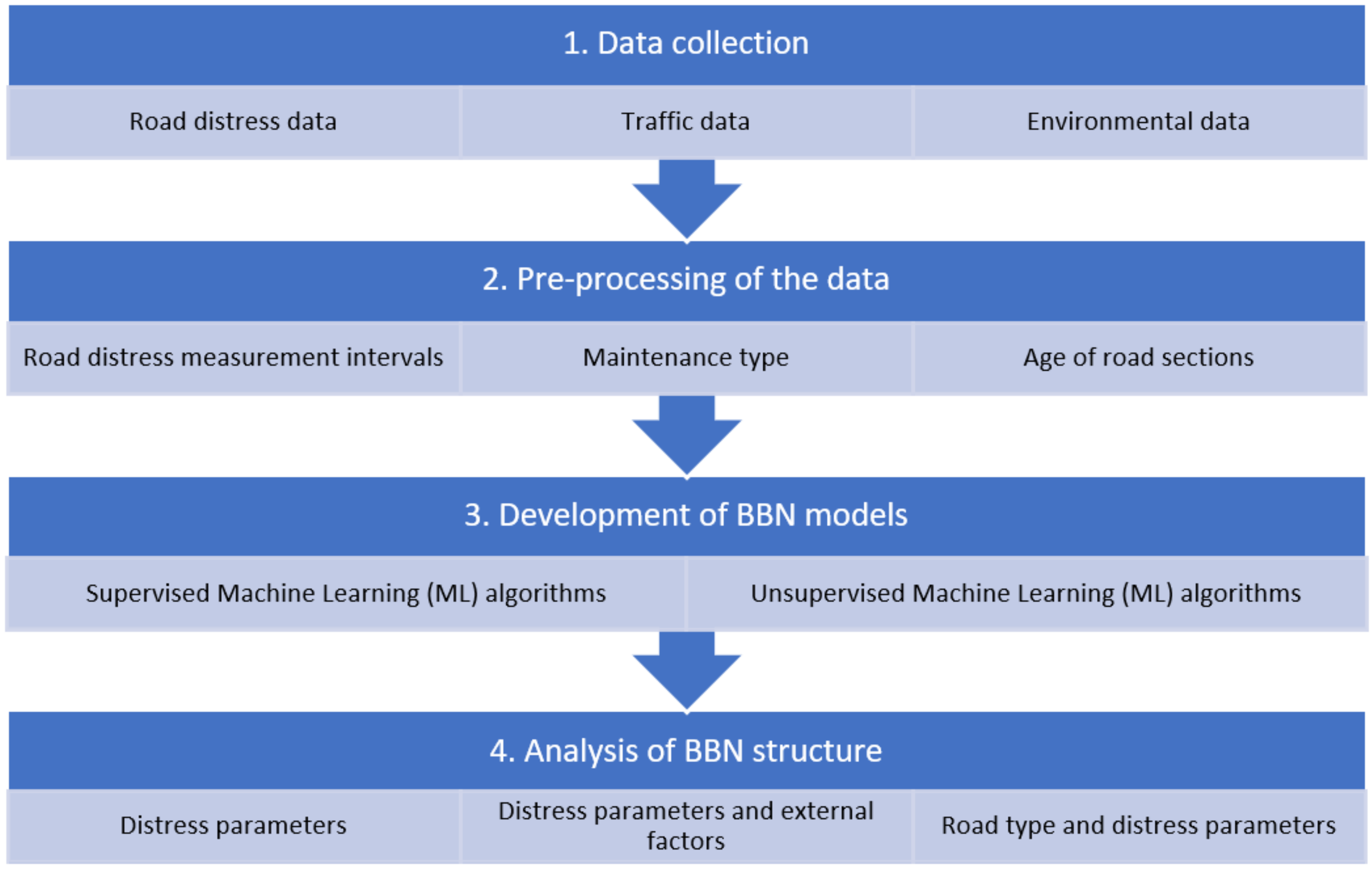
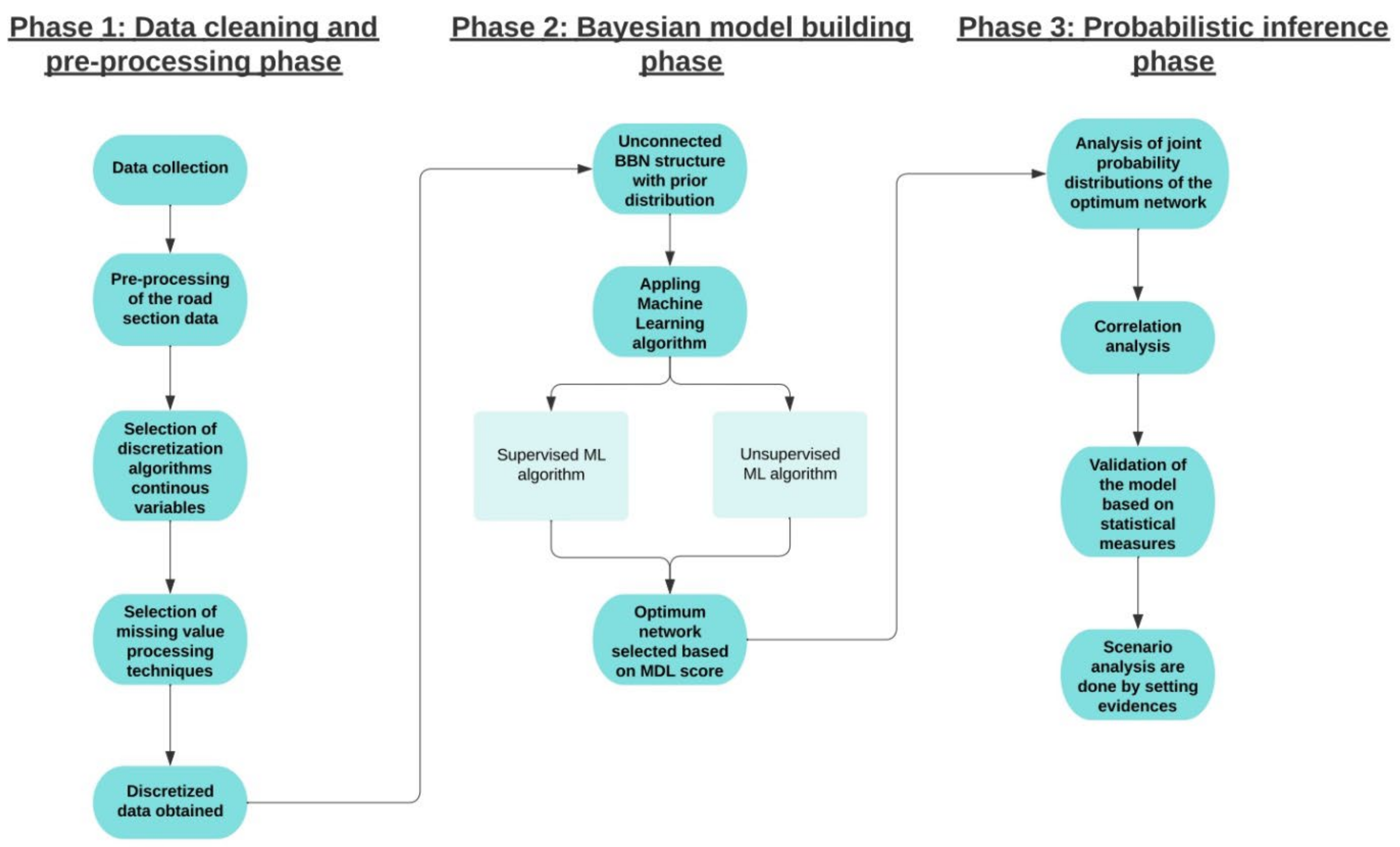
3. Methodology
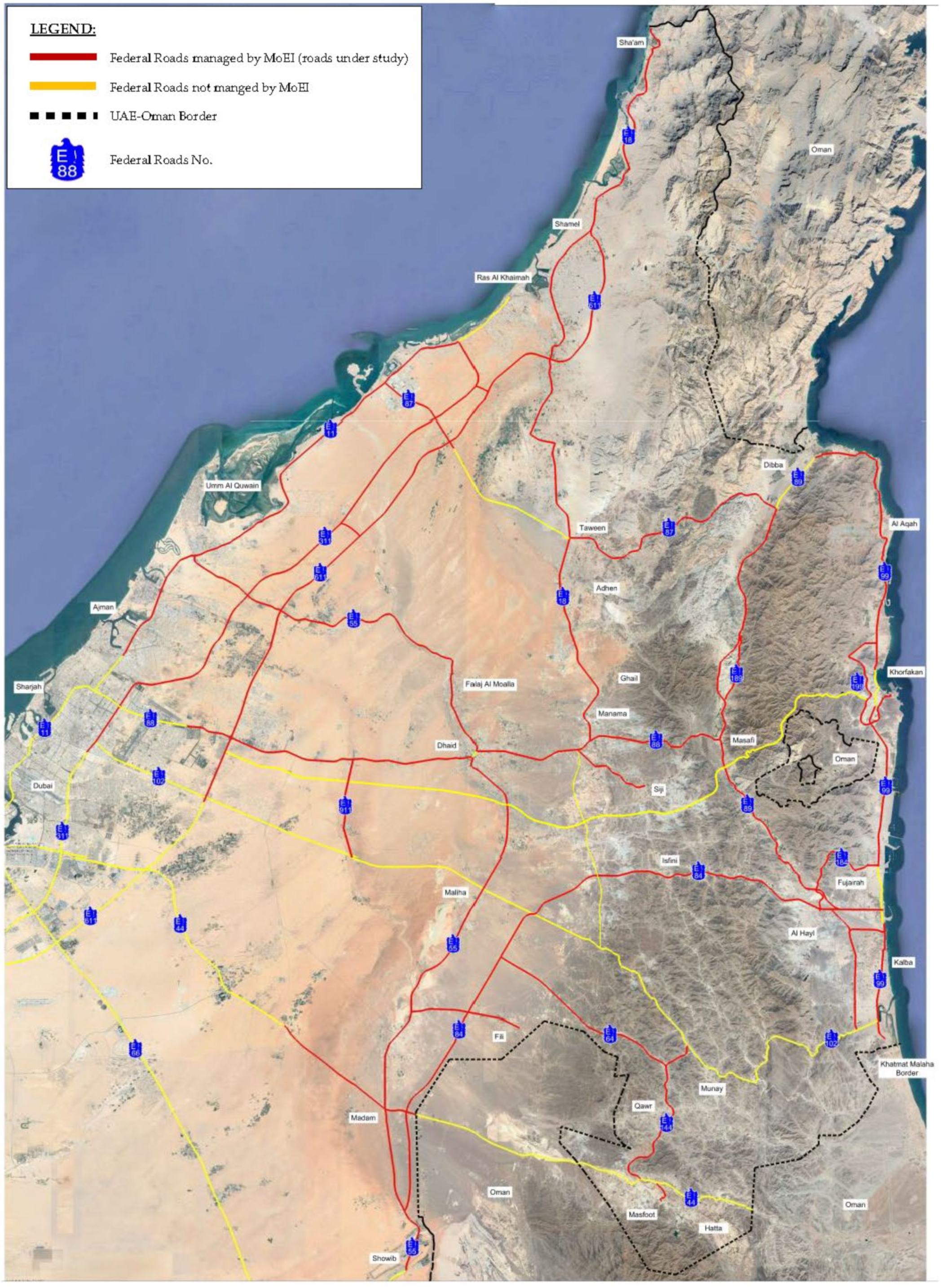
3.1. Data Collection
3.1.1. Road Data
- Cracking-Laser Crack Measurement System (LCMS);
- Deflection-Falling Weight Deflectometer (FWD);
- IRI-Laser profilometer;
- Rutting-Laser Rutting Measurement System.
3.1.2. Traffic Data
3.1.3. Environment Data
3.2. Pre-Processing of the Data
3.2.1. Road Distress Measurement Intervals
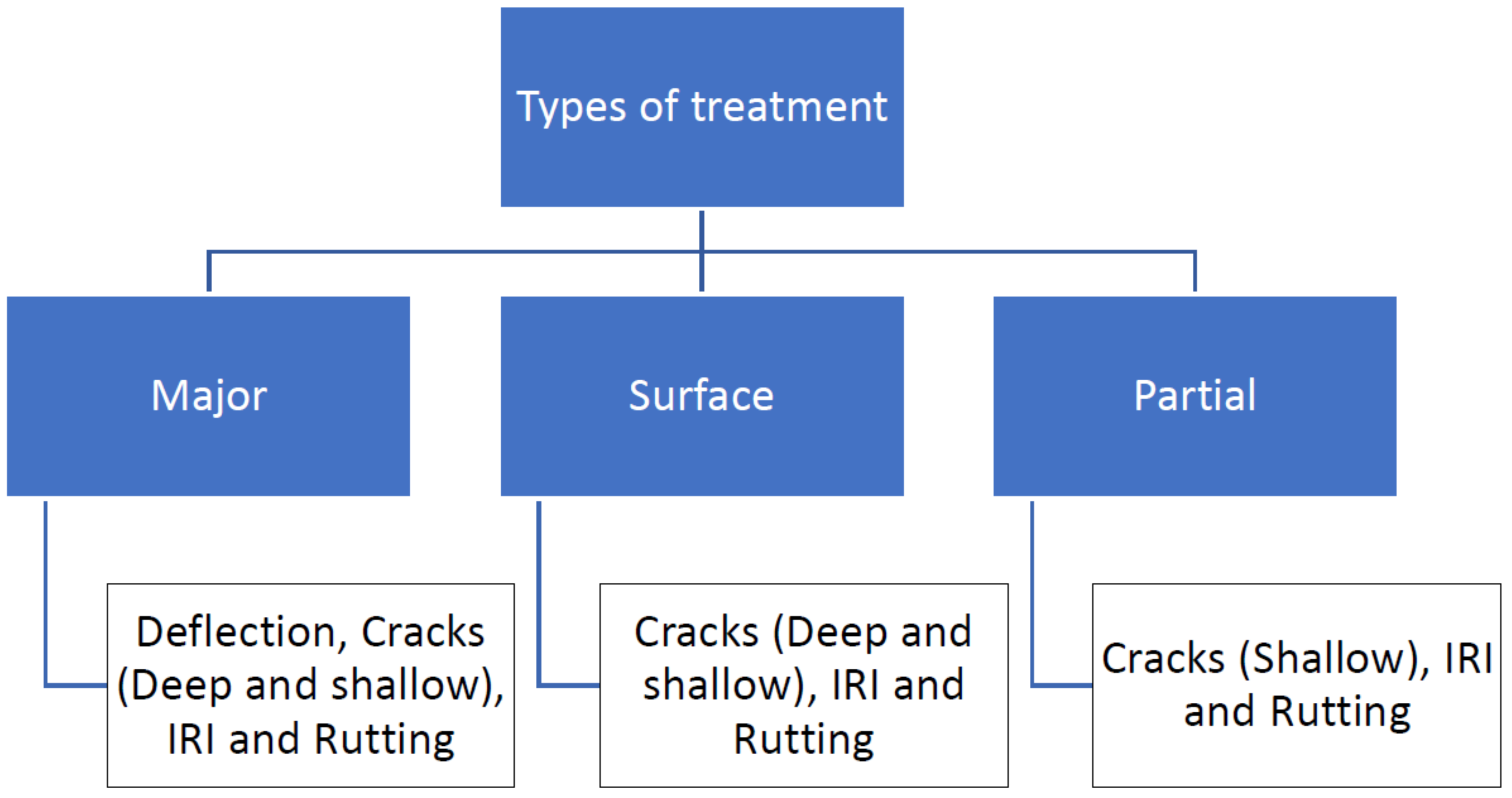
3.2.2. Assumption of Maintenance Treatment Types
3.2.3. Assumption of the Age of the Road Section
3.2.4. Prepared Data for Analysis
3.3. Development of BBN Model
3.3.1. Supervised and Unsupervised Bayesian Learning
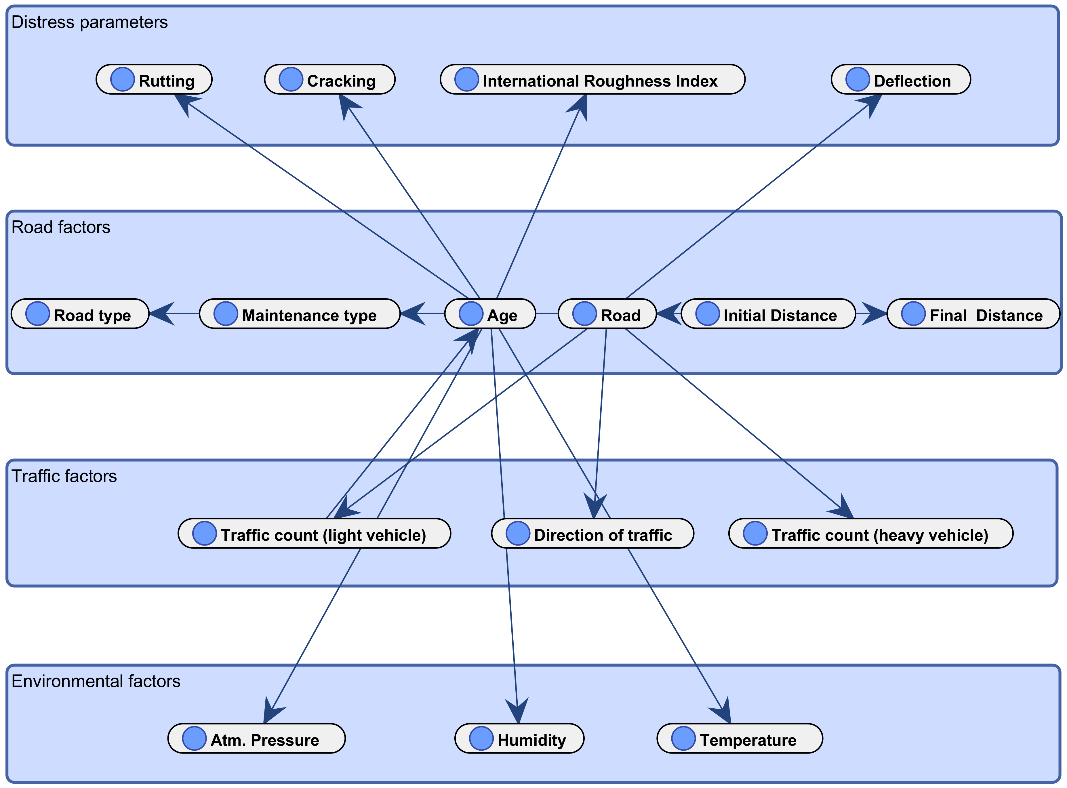
3.3.2. Proposed BBN Framework
3.4. Analysis of BBN Structure
3.4.1. Bayesian Correlation Analysis
3.4.2. Optimum Model Selection
4. Results
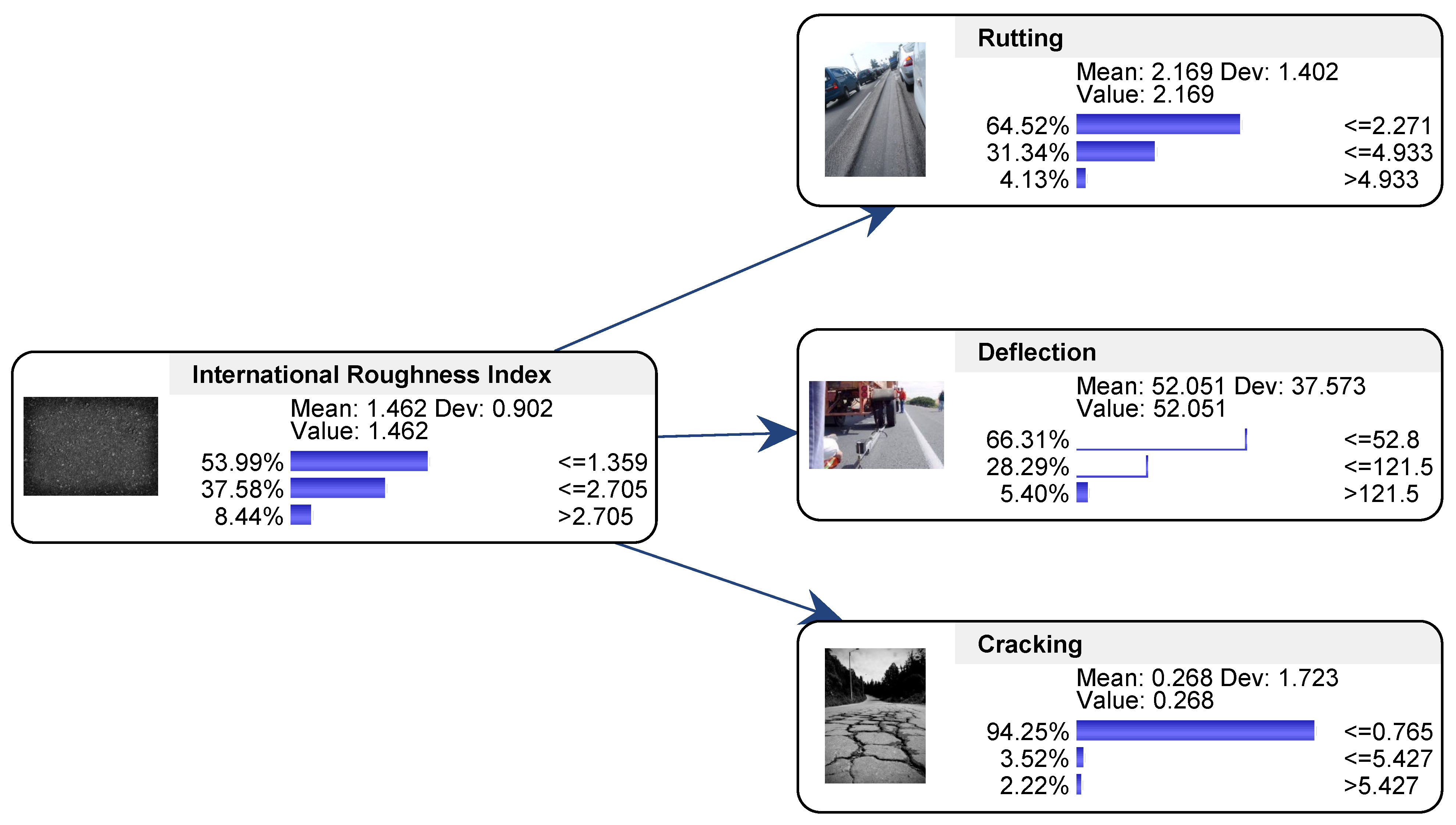
4.1. Correlation Analysis among Road Distress Parameters
- Entropy (H) = 3.7651;
- Normalized entropy (Hn) = 59.3873%;
- Hn(Complete) = 58.8520%;
- Hn(Unconnected) = 63.2849%;
- Contingency table fit = 87.9245%.
4.2. Correlation between Road Distress Parameters and External Factors
- Entropy (H) = 8.0357;
- Normalized entropy (Hn) = 33.8716%;
- Hn(Complete) = 30.3863%;
- Hn(Unconnected) = 65.4378%;
- Contingency table adjustment = 90.0567%.
4.3. Correlation between Road Type and Road Distress Parameters: Sensitivity Analysis
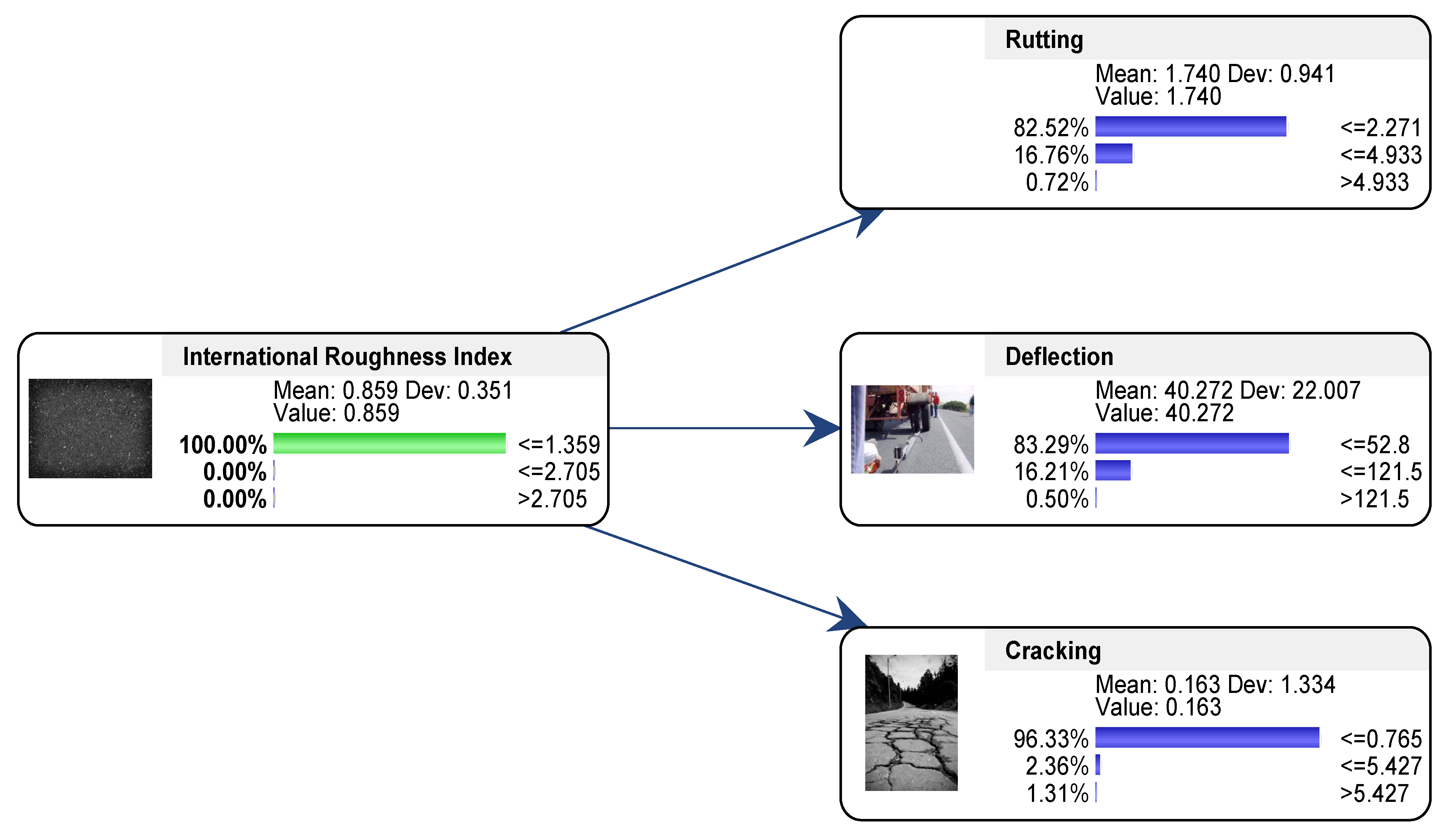
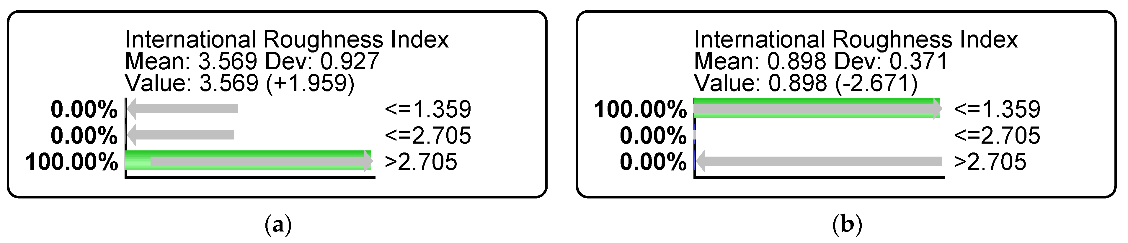
- Case 1: The probability of the distress parameter is set high, e.g., P(IRI > 2.705) = 100%, while the probability of the other three parameters is not changed (no evidence). This case is shown in Table 9 as IRI = high.
- For arterial roads, deflection and IRI are the prominent distresses with a difference of 20.91% and 19.55%, respectively.
- For collector roads, cracking is the most important with a difference of 7.22%.
- For expressways, deflection is the most important with a difference of 11.13%.
- For freeways, IRI is particularly pronounced with a difference of 19.59%.
5. Discussion and Future Scope
6. Conclusions
- Correlation analysis among road distress parameters revealed that IRI is strongly correlated with rutting and deflection, and it has a less significant correlation with cracking. IRI was found to be the central factor to represent overall pavement condition, which could be used as an indicator of the presence of rutting and deflection that generally progress at similar rates within the analysed UAE dataset. Further studies are needed to verify whether a similar trend is also generalizable for different countries
- The Bayesian analysis of road distress parameters and external factors unveiled the role of external factors in the development of road distress parameters. The BBN model developed in this paper indicated that the knowledge of external factors such as traffic, environment and road characteristics are capable to probabilistically estimating the values of road distress parameters at a higher accuracy without actually measuring them in the field.
- Sensitivity analyses revealed that the road distresses are sensitive to each road type (i.e., arterial, expressway, freeway and collector). Deflection and IRI were found to be prominent in arterial roads. Cracking was prominent in collector roads, deflection in expressways and IRI in freeways.
- Practically, these results provide the basis for optimizing road assessment data collection efforts and finding a compromise when it is not possible to obtain data about all distress factors. Since pavement deterioration factors are expressed as probability distributions in the developed Bayesian belief network models, road maintainers could adopt the proposed BBN approach to approximate the values of unknown road distress parameters even with the minimum available data.
Author Contributions
Funding
Acknowledgments
Conflicts of Interest
References
- Martin Rogers, B.E. Highway Engineering, 3rd ed.; John Wiley & Sons: Hoboken, NJ, USA, 2016. [Google Scholar]
- Bennett, C.R.; de Solminihac, H.; Chamorro, A. Data Collection Technologies for Road Management; World Bank: Washington, DC, USA, 2006; pp. 1–8. Available online: https://openknowledge.worldbank.org/handle/10986/11776 (accessed on 21 April 2022).
- Mcdaniel, R.; Shah, A. Asphalt additives to control cracking and rutting. Joint Transportation Research Program. January 2003. Available online: https://docs.lib.purdue.edu/cgi/viewcontent.cgi?article=1495&context=jtrp (accessed on 21 April 2022).
- Visintine, B.A.; Hicks, G.R.; Cheng, D.X.; Elkins, G.E.; Groeger, J. Factors Affecting the Performance of Pavement Preservation Treatments. In Proceedings of the 9th International Conference on Managing Pavement Assets, Washington, DC, USA, 18–21 May 2015; p. 23. Available online: https://vtechworks.lib.vt.edu/bitstream/handle/10919/56449/ICMPA9-000121.PDF (accessed on 21 April 2022).
- Ismail, M.A.; Sadiq, R.; Soleymani, H.R.; Tesfamariam, S. Developing a road performance index using a Bayesian belief network model. J. Franklin Inst. 2011, 348, 2539–2555. [Google Scholar] [CrossRef]
- Lin, J.; Yau, J.-T.; Hsiao, L.-H. Correlation Analysis Between International Roughness Index (IRI) by neural network. In Proceedings of the 82nd Annual Meeting of the Transportation Research Board, Washington, DC, USA, 12–16 January 2013; pp. 1–21. [Google Scholar]
- Gong, H.; Sun, Y.; Shu, X.; Huang, B. Use of random forests regression for predicting IRI of asphalt pavements. Constr. Build. Mater. 2018, 189, 890–897. [Google Scholar] [CrossRef]
- Mubaraki, M. Highway subsurface assessment using pavement surface distress and roughness data. Int. J. Pavement Res. Technol. 2016, 9, 393–402. [Google Scholar] [CrossRef] [Green Version]
- Chen, X.; Dong, Q.; Zhu, H.; Huang, B. Development of distress condition index of asphalt pavements using LTPP data through structural equation modeling. Transp. Res. Part C Emerg. Technol. 2016, 68, 58–69. [Google Scholar] [CrossRef]
- Fakhri, M.; Karimi, S.M.; Barzegaran, J. Predicting international roughness index based on surface distresses in various climate and traffic conditions using laser crack measurement system. Transp. Res. Rec. 2021, 2675, 397–412. [Google Scholar] [CrossRef]
- Hsieh, Y.-A.; Tsai, Y.J. Machine Learning for Crack Detection: Review and Model Performance Comparison. J. Comput. Civ. Eng. 2020, 34, 04020038. [Google Scholar] [CrossRef]
- Kabir, G.; Balek, N.B.C.; Tesfamariam, S. Consequence-based framework for buried infrastructure systems: A Bayesian belief network model. Reliab. Eng. Syst. Saf. 2018, 180, 290–301. [Google Scholar] [CrossRef]
- Attoh-Okine, N.O. Probabilistic analysis of factors affecting highway construction costs: A belief network approach. Can. J. Civ. Eng. 2002, 29, 369–374. [Google Scholar] [CrossRef]
- Starkova, O.; Gagani, A.I.; Karl, C.W.; Rocha, I.B.C.M.; Burlakovs, J.; Krauklis, A.E. Modelling of environmental ageing of polymers and polymer composites—durability prediction methods. Polymers 2022, 14, 907. [Google Scholar] [CrossRef]
- Park, E.; Chang, H.J.; Nam, H.S. A Bayesian network model for predicting post-stroke outcomes with available risk factors. Front. Neurol. 2018, 9, 699. [Google Scholar] [CrossRef]
- Gemela, J. Financial analysis using Bayesian networks. Appl. Stoch. Model. Bus. Ind. 2001, 17, 57–67. [Google Scholar] [CrossRef]
- De Campos, L.M.; Cano, A.; Castellano, J.G.; Moral, S. Bayesian networks classifiers for gene-expression data. In Proceedings of the 2011 11th International Conference on Intelligent Systems Design and Applications, Cordoba, Spain, 22–24 November 2011; pp. 1200–1206. [Google Scholar] [CrossRef] [Green Version]
- Tosun, A.; Bener, A.B.; Akbarinasaji, S. A systematic literature review on the applications of Bayesian networks to predict software quality. Softw. Qual. J. 2017, 25, 273–305. [Google Scholar] [CrossRef]
- Mohamed, M.; Tran, D.Q. Risk-based inspection for concrete pavement construction using fuzzy sets and bayesian networks. Autom. Constr. 2021, 128, 103761. [Google Scholar] [CrossRef]
- Mohamed, M.; Tran, D.Q. Risk-Based Inspection Model for Hot Mix Asphalt Pavement Construction Projects. J. Constr. Eng. Manag. 2021, 147, 04021045. [Google Scholar] [CrossRef]
- Al-Saadi, I.; Wang, H.; Chen, X.; Lu, P.; Jasim, A. Multi-objective optimization of pavement preservation strategy considering agency cost and environmental impact. Int. J. Sustain. Transp. 2021, 15, 826–836. [Google Scholar] [CrossRef]
- Van Koten, C.; Gray, A.R. An application of Bayesian network for predicting object-oriented software maintainability. Inf. Softw. Technol. 2006, 48, 59–67. [Google Scholar] [CrossRef] [Green Version]
- Kotu, V.; Deshpande, B. (Eds.) Chapter 4—Classification. In Data Science, 2nd ed.; Morgan Kaufmann, Elsevier: Cambridge, MA, USA, 2019; pp. 65–163. [Google Scholar] [CrossRef]
- Huelsenbeck, J.P.; Larget, B.; Miller, R.E.; Ronquist, F. Potential applications and pitfalls of Bayesian inference of phylogeny. Syst. Biol. 2002, 51, 673–688. [Google Scholar] [CrossRef] [Green Version]
- Little, R.J.; Rubin, D.B. Statistical Analysis with Missing Data; John Wiley & Sons: Hoboken, NJ, USA, 2002. [Google Scholar]
- Fang, H.; Xu, H.; Yuan, H.; Zhou, Y. Discretization of Continuous Variables in Bayesian Networks Based on Matrix Decomposition. In Proceedings of the 2017 International Conference on Computing Intelligence and Information System (CIIS), Nanjing, China, 21–23 April 2017; Volume 2018, pp. 184–187. [Google Scholar] [CrossRef]
- Furuya, T.; Ohbuchi, R. Transcoding across 3D shape representations for unsupervised learning of 3D shape feature. Pattern Recognit. Lett. 2020, 138, 146–154. [Google Scholar] [CrossRef]
- Myung, I.J. Computational Approaches to Model Evaluation. Int. Encycl. Soc. Behav. Sci. 2001, 2453–2457. [Google Scholar] [CrossRef]
- Bayesia. S.A.S. BayesiaLab. Available online: https://www.bayesia.com/ (accessed on 31 December 2021).
- Theodoridis, S. Probability and Stochastic Processes; Academic Press: Cambridge, MA, USA, 2020. [Google Scholar]
- Zhao, J.; Liang, J.M.; Dong, Z.N.; Tang, D.Y.; Liu, Z. Accelerating information entropy-based feature selection using rough set theory with classified nested equivalence classes. Pattern Recognit. 2020, 107, 107517. [Google Scholar] [CrossRef]
- Qiao, J.; Li, Y. Resource leveling using normalized entropy and relative entropy. Autom. Constr. 2018, 87, 263–272. [Google Scholar] [CrossRef]
- Clogg, C.C.; Rudas, T.; Matthews, S. Analysis of Contingency Tables Using Graphical Displays Based on the Mixture Index of Fit. In Visualization of Categorical Data; Academic Press: Cambridge, MA, USA, 1998; pp. 425–439. [Google Scholar] [CrossRef]
- Gerassis, S.; Albuquerque, M.; García, J.; Boente, C.; Giráldez, E.; Taboada, J.; Martín, J. Understanding complex blasting operations: A structural equation model combining Bayesian networks and latent class clustering. Reliab. Eng. Syst. Saf. 2019, 188, 195–204. [Google Scholar] [CrossRef]
- Prasad, J.R.; Kanuganti, S.; Bhanegaonkar, P.N.; Sarkar, A.K.; Arkatkar, S. Development of Relationship between Roughness (IRI) and Visible Surface Distresses: A Study on PMGSY Roads. Procedia-Soc. Behav. Sci. 2013, 104, 322–331. [Google Scholar] [CrossRef] [Green Version]
- Colombier, G. Cracking in pavements: Nature and origin of cracks. In Prevention of Reflective Cracking in Pavements; CRC Press: London, UK, 2004; pp. 14–29. [Google Scholar]
- Zavagna, P.; Khanal, A.; Souliman, M. LTTP Data Analysis: Factors Affecting Pavement Roughness for the State of California. J. Mater. Eng. Struct. 2018, 5, 319–332. [Google Scholar]
- Bhandari, S.; Luo, X.; Wang, F. Understanding the effects of structural factors and traffic loading on flexible pavement performance. Int. J. Transp. Sci. Technol. 2022, in press. [Google Scholar] [CrossRef]
- Alkaissi, Z.A. Effect of high temperature and traffic loading on rutting performance of flexible pavement. J. King Saud Univ.-Eng. Sci. 2020, 32, 1–4. [Google Scholar] [CrossRef]
- Von Quintus, H.L.; Simpson, A.L. Structural Factors for Flexible Pavements: Initial Evaluation of the SPS-1 Experiment Final Report; No. FHWA-RD-01-166; Federal Highway Administration: Washington, DC, USA, 2003. Available online: https://rosap.ntl.bts.gov/view/dot/41562 (accessed on 21 April 2022).
- Li, R.; Schwartz, C.W.; Forman, B. Sensitivity of Predicted Pavement Performance to Climate Characteristics. In Proceedings of the Airfield and Highway Pavement 2013: Sustainable and Efficient Pavements, Los Angeles, CA, USA, 9–12 June 2013. [Google Scholar] [CrossRef]
- Pais, J.C.; Amorim, S.I.; Minhoto, M.J. Impact of Traffic Overload on Road Pavement Performance. J. Transp. Eng. 2013, 139, 873–879. [Google Scholar] [CrossRef]
- Mamlouk, M.; Vinayakamurthy, M.; Underwood, B.S.; Kaloush, K.E. Effects of the International Roughness Index and Rut Depth on Crash Rates. Transp. Res. Rec. 2018, 2672, 418–429. [Google Scholar] [CrossRef]
- Uusitalo, L. Advantages and challenges of Bayesian networks in environmental modelling. Ecol. Modell. 2007, 203, 312–318. [Google Scholar] [CrossRef]
- Wasserman, L. Bayesian Inference. In All of Statistics; Springer Texts in Statistics; Springer: New York, NY, USA, 2004. [Google Scholar] [CrossRef]


| Distress Factor | Unit | Measuring Interval in Meters | Minimum Value | Maximum Value |
|---|---|---|---|---|
| Cracking | Percentage (%) | 10 | 0.00 | 99.87 |
| Deflection | mm/100 | 100 | 0.00 | 374.00 |
| IRI | m/km | 10 | 0.00 | 52.99 |
| Rutting | Mm | 10 | 0.00 | 52.65 |
| Before Pre-Processing | After Pre-Processing | ||
|---|---|---|---|
| Initial Distance | Final Distance | Initial Distance | Final Distance |
| 651 | 672 | 660 | 670 |
| Road Data | Distress Parameters | Environment Factors | Traffic Factors | ||||||||||||
|---|---|---|---|---|---|---|---|---|---|---|---|---|---|---|---|
| Road | Road Type | Initial Distance | Final Distance | Maintenance Type | Age | Cracking | Deflection | IRI | Rutting | Temperature | Humidity | Atm. Pressure | Traffic Count (Light Vehicle) | Traffic Count (Heavy Vehicle) | Traffic Direction |
| E11 | Arterial | 8540 | 8550 | Partial | 1 | 0 | 51 | 1.016 | 1.75375 | 26 | 49 | 1019 | 4,203,429 | 487,421 | Forward |
| Machine Learning Algorithm | Discretization Algorithm | Discretization Interval | Missing Value Processing Method | MDL Score |
|---|---|---|---|---|
| Maximum Spanning Tree | R2 GenOpt* | 3 | Dynamic Imputation | 20,547.234 |
| Taboo | R2 GenOpt* | 3 | Dynamic Imputation | 20,493.881 |
| EQ | R2 GenOpt* | 3 | Dynamic Imputation | 18,311.781 |
| TabooEQ | R2 GenOpt* | 3 | Dynamic Imputation | 20,493.881 |
| SopLEQ | R2 GenOpt* | 3 | Dynamic Imputation | 20,493.881 |
| Taboo Order | R2 GenOpt* | 3 | Dynamic Imputation | 20,493.881 |
| Maximum Spanning Tree | R2 GenOpt* | 4 | Dynamic Imputation | 24,668.868 |
| Taboo | R2 GenOpt* | 4 | Dynamic Imputation | 24,615.515 |
| EQ | R2 GenOpt* | 4 | Dynamic Imputation | 22,9140.438 |
| TabooEQ | R2 GenOpt* | 4 | Dynamic Imputation | 24,615.515 |
| SopLEQ | R2 GenOpt* | 4 | Dynamic Imputation | 24,615.515 |
| Taboo Order | R2 GenOpt* | 4 | Dynamic Imputation | 24,615.515 |
| Parent | Child | KL Divergence | Overall Contribution | Mutual Information | Pearson’s Correlation |
|---|---|---|---|---|---|
| International Roughness Index | Rutting | 0.1470 | 49.2141% | 0.1470 | 0.4249 |
| International Roughness Index | Deflection | 0.1429 | 47.8553% | 0.1429 | 0.4218 |
| International Roughness Index | Cracking | 0.0088 | 2.9306% | 0.0088 | 0.1025 |
| Node | Outgoing Force | Incoming Force | Total Force |
|---|---|---|---|
| International Roughness Index | 0.2986 | 0.0000 | 0.2986 |
| Rutting | 0.0000 | 0.1470 | 0.1470 |
| Deflection | 0.0000 | 0.1429 | 0.1429 |
| Cracking | 0.0000 | 0.0088 | 0.0088 |
| Features | Values |
|---|---|
| Road type | Arterial |
| Direction of traffic | Forward |
| Temperature | 26 |
| Humidity | 49 |
| Atm. Pressure | 1019 |
| Traffic count (light vehicle) | 4,203,429 |
| Traffic count (heavy vehicle) | 487,421 |
| Maintenance type | Partial |
| Age from last maintenance | 1 |
| Road | E11 |
| Initial distance | 8540 |
| Final distance | 8550 |
| Cracking | 0 |
| Deflection | 51 |
| International Roughness Index | 1.016 |
| Rutting | 1.75375 |
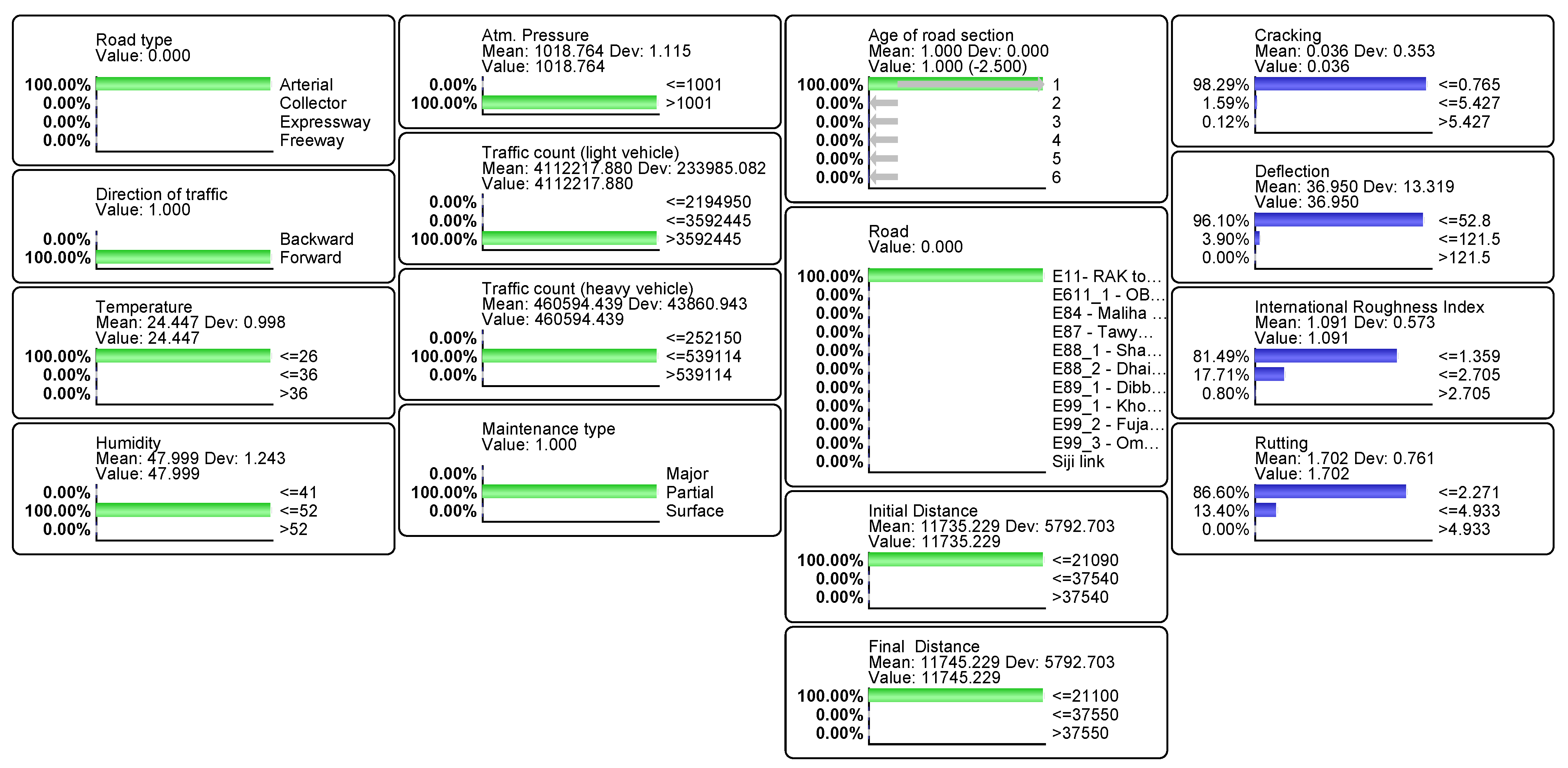
| Variable | Actual Value | Bayesian Inference | Probability of Occurrence |
|---|---|---|---|
| Cracking | 0 | <=0.765 | 98.29% |
| Deflection | 51 | <=52.8 | 96.10% |
| International Roughness Index | 1.016 | <=1.359 | 81.49% |
| Rutting | 1.75375 | <=2.271 | 86.60% |
| States (Road Types) | IRI | Rutting | Deflection | Cracking | ||||
|---|---|---|---|---|---|---|---|---|
| Low | High | Low | High | Low | High | Low | High | |
| Arterial | 56.9683% | 76.5180% | 72.5815% | 82.6908% | 70.8836% | 91.7979% | 70.1623% | 66.6197% |
| Collector | 3.2154% | 4.4249% | 1.4362% | 4.9982% | 1.6350% | 1.6369% | 2.8507% | 10.0693% |
| Expressway | 4.7211% | 3.5550% | 1.9244% | 1.5604% | 11.1251% | 0.0000% | 7.3121% | 8.6105% |
| Freeway | 35.0952% | 15.5021% | 24.0580% | 10.7505% | 16.3563% | 6.5651% | 19.6748% | 14.7006% |
Publisher’s Note: MDPI stays neutral with regard to jurisdictional claims in published maps and institutional affiliations. |
© 2022 by the authors. Licensee MDPI, Basel, Switzerland. This article is an open access article distributed under the terms and conditions of the Creative Commons Attribution (CC BY) license (https://creativecommons.org/licenses/by/4.0/).
Share and Cite
Philip, B.; Jassmi, H.A. A Bayesian Approach towards Modelling the Interrelationships of Pavement Deterioration Factors. Buildings 2022, 12, 1039. https://doi.org/10.3390/buildings12071039
Philip B, Jassmi HA. A Bayesian Approach towards Modelling the Interrelationships of Pavement Deterioration Factors. Buildings. 2022; 12(7):1039. https://doi.org/10.3390/buildings12071039
Chicago/Turabian StylePhilip, Babitha, and Hamad Al Jassmi. 2022. "A Bayesian Approach towards Modelling the Interrelationships of Pavement Deterioration Factors" Buildings 12, no. 7: 1039. https://doi.org/10.3390/buildings12071039