A Case Study of Mapping the Heating Storage Capacity in a Multifamily Building within a District Heating Network in Mid-Sweden

Abstract

The building sector accounts for a third of the total energy use in Sweden, and district heating provides half of the heating needs. The peak demand loads within a district heating network occur both regularly and irregularly and impose a burden on the energy company to fulfill the demand, often by using more expensive and less environmentally friendly resources (e.g., fossil fuels) instead of the waste heat from industry or biofuels. Heat storage during hours of less demand and prior to colder periods can be used for load management and sustainable planning of energy supply, as well as reduction of total greenhouse gas emissions. Thus, heat supply to the building can be lowered temporarily during the peak power period to utilize the stored thermal energy within the building thermal inertia. The use of indoor temperature decay and the delivery of heating power to a multifamily building are studied here, and heating storage capacity and thermal inertia are calculated. During the performed decay test, the energy supply was estimated to be reduced by 61% for 5 h, which resulted in only a 0.3 °C temperature decay. Therefore, the suggested method can shave eventual peaks in supplied heat with minimal influence on the thermal comfort.

1. Introduction

Climate change is one of the main concerns of the modern era, and reducing net emissions is crucial to mitigating greenhouse gas (GHG) emissions, mainly CO₂, and their consequences. The building sector stands for approximately one third of the total energy use worldwide [1] and 39% of the total GHG emissions [2]. The sector involves challenges such as population growth, global warming, extreme heat and cold waves, energy transition from fossil fuels to renewable ones, availability of primary energy sources, and related GHG emissions. Thus, reducing the building sector energy demand is a crucial part of energy suppliers being able to ensure a sustainable future in compliance with the United Nations sustainability goals, which includes renewable energy and a clean environment [3]. Because of this, the environmental impacts of GHG emissions [4] shifted global attention to the efficient use of resources and considering the primary energy use rather than final energy use only. Moreover, policy makers in the European Commission presented climate action and climate-protecting laws, such as the so-called European Green Deal, to mitigate the GHG emissions by 55% by 2030 (compared to 1990 levels) and make the EU more climate neutral by 2050 [5,6].

Buildings in Sweden account for approximately 21% of the Sweden’s greenhouse gas emissions. Sweden has a goal for zero net emissions by 2045, and there is a great need to reduce the energy and heat demand of buildings. Approximately 50% of the total heating (both space heating and domestic tap water) for all types of buildings in Sweden is supplied by district heating. The share is more than 90% for multifamily buildings. In Sweden, district heating (DH) is gained from the waste heat from industry, geothermal heat, combined heat and power (CHP) plants burning biofuels, and incineration, and the total level of GHG emission is approximately 53.7 g CO₂eq/kWh [7]. However, the DH demand is not evenly distributed, and especially during peak hours, fossil fuels might be used to fulfill the demand of the DH networks [8].

There are more than 200 district heating companies in Sweden [9], and some weight the tariffs for the subscribed heating power demand with penalties for customers who exceed the subscribed power and have extra peak loads. DH load data history gives a better understanding of the DH network and reveals the customer demand and behavior throughout different periods including the peak hours [10]. The peak demand can be during temporarily extreme cold weather conditions, or higher demands can be during peak hours in the mornings and evenings, as well as some abnormal peak loads on other occasions. There are also especially some irregular peak hours with individual larger buildings (offices or multifamily buildings). Peak loads within a district occur both regularly and irregularly and these also impose a burden on the energy company to supply and fulfill the demand, and, often, more expensive resources are used which can be less environmentally friendly (normally by using fossil fuels) in comparison to the waste heat from industry or CHP plants which burn biofuel or incineration. In addition, it is more rewarding for building owners to manage their energy use so that the peak demands can be avoided. Moreover, energy suppliers can plan and manage their production in a more sustainable ways to reduce GHG emissions. The load management and energy storage are important elements of the modern district heating network, 4th generation, and increase its efficiency and reliability considering more environmental resources. Lund et al., reviewed the status of the 4th generation DH and concluded that the DH should be integrated with more energy efficient buildings and lower the supply and return temperatures in the network [11]. In a so-called smart thermal grid, the buildings in a DH district can also store and release energy in the network [12]. Additionally, as the heat demand is increasing in the residential sector, the competitiveness of DH can be increased by using a more efficient DH network [13]. In the modern DH network, the temperature in the primary distribution line is strived to be kept at a minimum and to achieve lower return temperatures, and thus improve the quality and efficiency of the whole network, i.e., not only improving the efficiency in the production side but also in the demand side [14].

There are different load management methods for shaving the top heating load peaks in district heating networks, including different thermal storage systems and based on weather or user behavior predictions [15]. For instance, the DH supplied to the building can be stored in the building structures (or thermal batteries such as water tanks) during periods before upcoming cold weather, and thus the stored heat can be released and used later, when there is larger demand for the DH supply. This will contribute to a more uniform DH demand in the network and also increase the flexibility in the DH network through the control of DH supply [16]. Thanks to the heat released from the building thermal mass, lowering the district heating supply will not affect the indoor temperature dramatically, depending on the period length of the load management. Sven Werner analyzed the daily heat load pattern of six DH networks in Sweden and developed a model for optimizing the heat supply for both space heating and domestic hot water. He discussed that the eventual bias in the model can be reduced for instance by having more accurate input data [17]. Furthermore, Gadd and Werner studied the heat load variations in the DH network and estimated the size of heat storage in order to remove the heat load variations [18]. The same authors also categorized the heat load pattern by analyzing the hourly DH data for 141 DH substations, including both multi-dwelling as well as commercial premises, and pointed to the large variation in the heat load pattern between the connected buildings [19].

In addition to studies performed on detecting and analyzing the heat load patterns and optimizing the DH distribution [17,18,19], data driven approaches were used to discover the heat load patterns in DH networks. For instance, Calikus et al. presented a large-scale automatic data-driven method for analyzing the heat load patterns and they implement the method for detecting the load pattern of 1222 DH-connected buildings [20]. Additionally, Buffa et al. did a review on the control strategies for demand response and peak shaving in a DH network focusing on low temperature DH supply. They pointed to the efficient use of machine learning in more advanced control strategies such as predictive and multi-agent systems [21]. The energy signature method is also studied in order to analyze and estimate the heat load demand as well as the heat loss coefficients of the buildings. For instance, Eriksson et al., compared the heat loss coefficient of a multi-family building both before and after renovation using the energy signature methods, i.e., analyzing the annual delivered DH versus the outdoor temperature [22]. Using the same method, they also estimated the domestic hot water and the balance temperature of the building. Nordström et al. also used the energy signature method to estimate the total U-value of six single-family buildings and proved that effective U-values can be calculated by having a large enough indoor–outdoor temperature difference [23]. Different demand side management control strategies of using building structures for thermal storage, especially TABS (thermally activated buildings systems) are also studied by Arteconi et al., and suggest high potential for using TABS in order to shave the heat load peaks [24].

However, the efficiency of the load management method depends on the storage capacity in the DH network. Building structures can be used as short-term storage thermal batteries, i.e., by varying the indoor temperature; heat can be stored within the structure and can be released in colder periods—thus, the delivered DH will be lowered at peak hours depending on the building’s thermal inertia. Johansson et al. proposed a multi-agent control system using the building structure for heat storage and optimization in the production units [25]. They showed that the method can reduce or remove the peak loads in a DH network, which increases the profits for the energy company and reduces the GHG emissions. Building structures can be assumed as free and available thermal storages that lead to cheaper energy storage in comparison to other active thermal and electrical battery storages; and integrated use of energy storage within building structures is a crucial part of the cost-effective sustainable energy systems of the future [26]. Turski and Sekret studied the heat storage capacity of buildings and the DH network in order to mitigate the delivered heat [27]. They showed that using the thermal storage capacity of building structures together with the DH network can reduce up to 14.8% of the heat output, mainly for the central space heating. The thermal capacity and heat storage of the DH network were governed by raising the water temperature in the network, and the study confirmed that the heat storage in building structures is more operatable and feasible in comparison with the heat storage in the DH network itself.

The use of different thermal storage and control systems in order to increase the flexibility of smart energy grids and district heating and cooling networks is reviewed and studied by [18,28]. For instance, Masy et al. studied the grid flexibility using heat pumps and heat storage in building structures for the Belgian electricity smart grids, as Belgian residential buildings often use air to water electricity-driven heat pumps. They showed that control strategies for the smart grid can reduce the procurement and consumer costs while maintaining acceptable thermal comfort levels [28]. Furthermore, Glenn Reynders studied the effect of design parameters on structural thermal energy storage for active demand response in residential buildings [29]. He showed that the intelligent use of thermal heat storage can shave the peak loads and, in combination with the use of heat pumps and renewable energies sources, reduce the GHG emissions. In addition, Kensby et al. studied the building time constant as a characteristic of the thermal inertia and short-term storage capacity of the DH-connected buildings [30]. They used a varying building time constant instead of a mean value and showed that heavy concrete buildings can withstand larger variations in the delivered DH without dramatically affecting the indoor temperature and thermal comfort. Furthermore, forecast control systems were developed to predict and regulate the heat supply based on, e.g., the indoor–outdoor temperature, as well as the user behavior factors. For instance, Cholewa et al., studied a forecast control system for the space heating of a multi-family dwelling and an office building, proving more than 15 and 24% energy savings, respectively. The studied control system had the advantage of being installed in less than two hours, and therefore could be widely and cost effectively used even for existing buildings [31]. There are also studies based on regression models, for instance, Bilous et al., developed a non-linear multivariable regression (MLR) model for the predication of the indoor temperature based on (for instance) heating load, ventilation rate, outdoor temperature, wind speed, and solar heat gains [32]. The model was developed based on simulations with EnergyPlus and constant coefficients were calculated for each influencing parameter of the studied building model so the authors could present high accuracy of such MLR models for the simulated building model.

In Sweden, the use of DH must be monitored every hour to serve as a basis for energy bills [33]. Moreover, property owners are increasingly installing at least one temperature sensor per apartment to trace adverse indoor thermal conditions or to prove to complaining tenants that the indoor temperature is satisfactory. These gathered data can be used for more purposes than those listed above. For example, the energy signature method provides a means of assessing the heat loss coefficient and balance temperature of a building, and can be utilized on a large scale (e.g., buildings in a neighborhood/district). However, it does not give information on how the thermal inertia of the building, which is needed to map the indoor temperature drop if the DH supply is reduced or cut during shorter periods, affects the total heat storage capacity of the building structure. This study explores how the mapping can be performed by combining an energy signature method together with the concept of a time constant. This is feasible by having access to historic DH supply data and an occasion when DH supply is reduced/cut for several hours. This provides an easily operatable, cheap, and non-intrusive method for calculating the building time constant and storage capacity by temporarily lowering the delivered energy. In a case study of one building, the use of energy signatures and time constants are tested against by stopping DH space heating for 5 h. The results are evaluated against a validated building energy simulation model in IDA-ICE.

2. Theory

In a DH network, the hot water (as the fluid medium in the DH distribution network) may be generated using the excess heat produced in a CHP plant or the waste heat from industry. DH is distributed to customers, such as buildings encompassing residential buildings, hospitals, schools, restaurants, etc., via the so-called primary piping network; and via the heat exchangers in each DH central, DH is delivered to the connected building(s) through secondary pipelines. An increased number of buildings connected to the network implies that more DH can be used and the return temperature will be decreased, which increases the total efficiency of the DH network. DH load is affected by the energy demands of the buildings, which are affected by the indoor–outdoor temperature difference, solar irradiation, and occupants’ use of appliances and lighting, as well as the type of activities inside the buildings. The peak loads in the DH network might occur due to the increase in domestic hot tap water use, colder outdoor weather conditions, or other user-related demands.

District heating delivered to the DH central is slightly higher than the DH demand and use in the building, because there are some losses through the heat exchanger in the DH central unit and pipes on the secondary side. Thus, the focus of this study is the delivered or supplied DH, which is measured and audited by the energy company.

2.1. Designed Power Requirement for Space Heating System

The designed or dimensioned heating power required for a building can be calculated by Equation (1) [34]:

$$P_{dim}=\left[\left({{\displaystyle \sum }}^{ }{U}_i·A_i+{{\displaystyle \sum }}^{ }{\Psi }_{TB k}·l_k+{{\displaystyle \sum }}^{ }{\chi }_l\right)+\left(\left(1-{\eta }_t\right)·F+F_{leakage}\right)·{\rho }_{air}·c_{air}\right].\left(T_i-DVUT\right) [\mathrm{W}]$$

(1)

where $U_i$ and $A_i$ are the transmission loss coefficients and areas of each envelope part, ${\Psi }_{TB k}$ and $l_k$ are the linear loss coefficients and lengths of thermal bridges, ${\chi }_l$ representing point thermal bridges, $F$ and $F_{leakage}$ are ventilation and air leakage flows, ${\rho }_{air}$ is air density, and $c_{air}$ is the specific heat capacity of air. $T_i$ is indoor temperature and DVUT (design winter outdoor temperature) is the n-day mean air temperature. DVUT is the maximum value of the 30 minimum n-day mean air temperature during a 30-year measuring period [35]. To determine DVUT, the heat stored in the building structures should be considered through the building time constant, $\tau$_b, expressed in hours or a 24 h period (n-day). The n-day mean air temperature (DVUT) (°C) for 1–4 days (and nights) for Gävle, location of the case study in this paper, can be found in [35].

2.2. Building Time Constant

The time constant of a heated building, τ_b, represents the internal thermal inertia of the building [36]. τ_b, is counted in hours (24 h = light building, 96 h = very heavy building). The heat stored in the entire building (internal and external structures) should be considered via the building time constant, τ_b, see Equation (2).

$${\tau }_b=\frac{C_{internal}}{H_t+H_v}=\frac{{{\displaystyle \sum }}^{ }{\rho }_m·c_m·V_m}{\left({{\displaystyle \sum }}^{ }{U}_i·A_i+{{\displaystyle \sum }}^{ }{\Psi }_{TB k}·L_k+{{\displaystyle \sum }}^{ }{\chi }_l\right)+\left(\left(1-{\eta }_t\right)·F+F_{leakage}\right)·{\rho }_{air}·c_{air}} [\mathrm{h}]$$

(2)

$C_{internal}$ is the sum of the thermal capacity of the building materials enclosed within the structure’s thermal insulation and no more than 100 mm of the construction layer that is exposed to the indoor space. $H_t$ and $H_v$ are the transmission and ventilation loss coefficients. ${\rho }_m$, $c_m$, and $V_m$ are the density, specific heat capacity, and volume of each construction layer, respectively.

In case of a sudden change in supplied heat, the indoor temperature will drop, provided that the outdoor temperature is constant. Indoor temperature decay is exponential according to Equation (3).

$$T_t=T_{\infty }+\left(T_0-T_{\infty }\right)·e^{-\frac{t}{{\tau }_b}} [\text{℃}]$$

(3)

$T_0$ is the initial temperature and $T_{\infty }$ is the final temperature. When internal heat loads are not considered, $T_{\infty }$ can be the outdoor temperature. $T_t$ is the temperature at time t, after the change was imposed. When $t={\tau }_b$, building time constant, is achieved, the temperature decreased to $\left(1-e^{-1}\right)\approx 0.63$ (i.e., 63%) of the total temperature difference between the steady state conditions.

3. Methods

Indoor temperature and delivered power data history (monitored and measured data) of a multifamily building with a total heated area of 2830 m² located in Gävle, mid Sweden, owned by the municipality housing company Gavlegårdarna AB, was used in order to audit the energy storage. It was built in 1965 and is located in Sweden. The building contains five floors and 27 apartments (see Figure 1). The building was simulated by IDA-Indoor Climate and Energy (IDA-ICE) simulation software version 4.8 in order to model the temperature decay and supplied heat within the apartments. Each apartment was simulated as a single zone and the average results for all apartments are studied here. IDA-ICE is a node-based simulation program used to model the building energy use and its indoor environment [37]. The software’s functionality and reliability are validated in different studies [38,39,40]. The simulation model of the multifamily building, studied in this paper, was calibrated and validated by Eriksson et al. [22]. The building experienced renovations during 2015–2016, which included changes of balconies, additional external insulation, new windows, and a mechanical ventilation system with heat recovery.

The building is connected to district heating and 184 MW was delivered by the local energy company, Gävle Energi AB, in 2017. In a basement room, there is a digitalized DH central unit (DUC) by which the temperature of the delivered DH is controlled and measured. Inside each DH central unit, there is a heat exchanger, which receives heat from the primary side and delivers it to the secondary side. The DUC is installed in the primary side and heat exchange is governed by outdoor temperature.

Some tests were performed in the DH network, where the local energy company, Gävle Energi AB, temporarily lowered the DH supply temperature in order to test peak power reduction by increasing the DUC’s outdoor sensor’s signal with +15 °C, i.e., “exposing” the heating system to a warmer outdoor temperature for 5 h. Indoor temperatures were monitored during the test to see the effect on the indoor temperatures of some connected building blocks—the sensors (one per apartment) are a part of the buildings energy management system (BEM). In the performed experiment, the indoor temperature decreased during 04:00–09:00 on a winter day (21 December 2017). The averaged indoor temperature of all the apartments is used in this study.

The available measured data include:

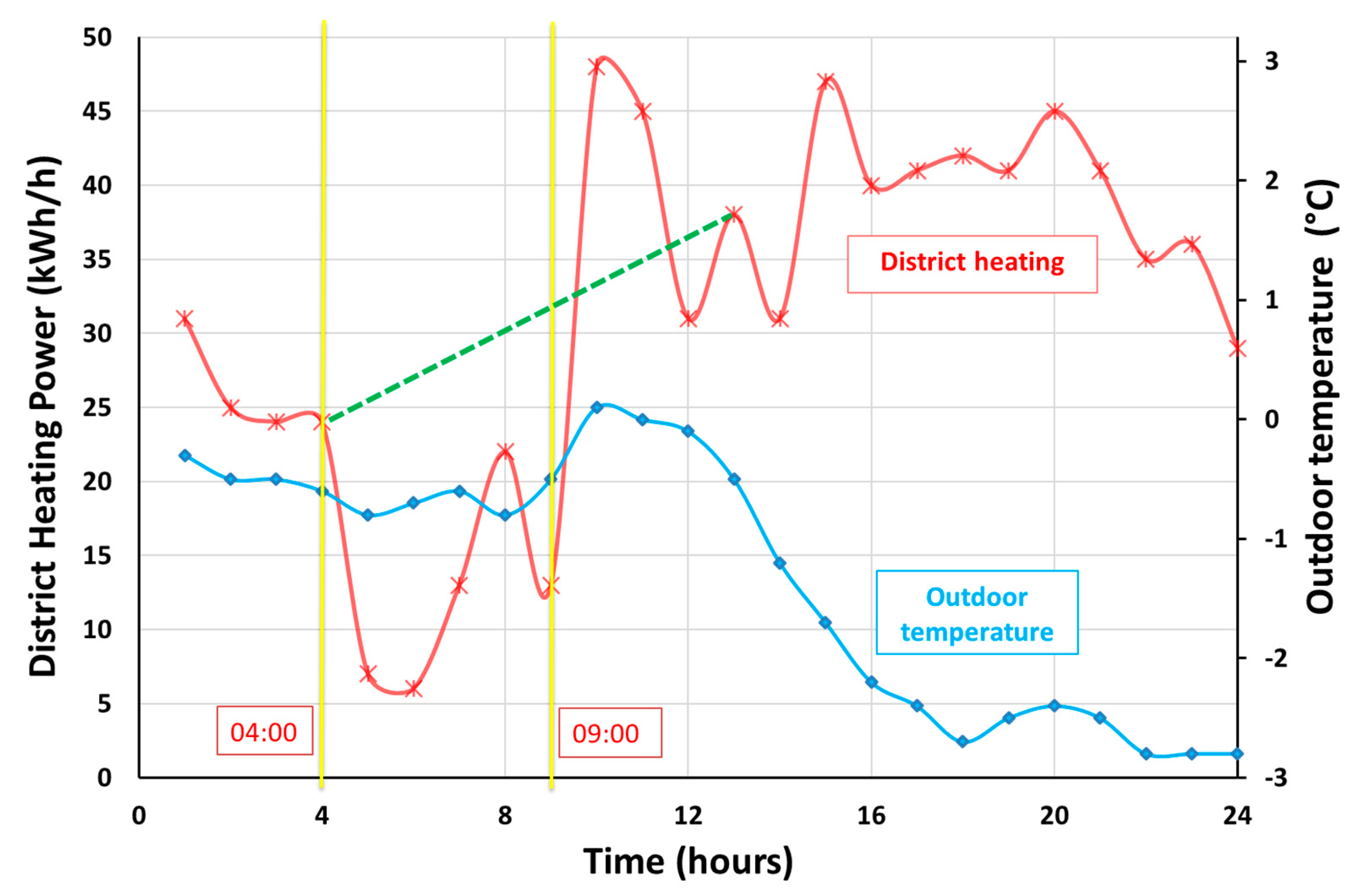
• Delivered hourly DH power (kWh/h) for the whole building—space and domestic hot water heating combined.
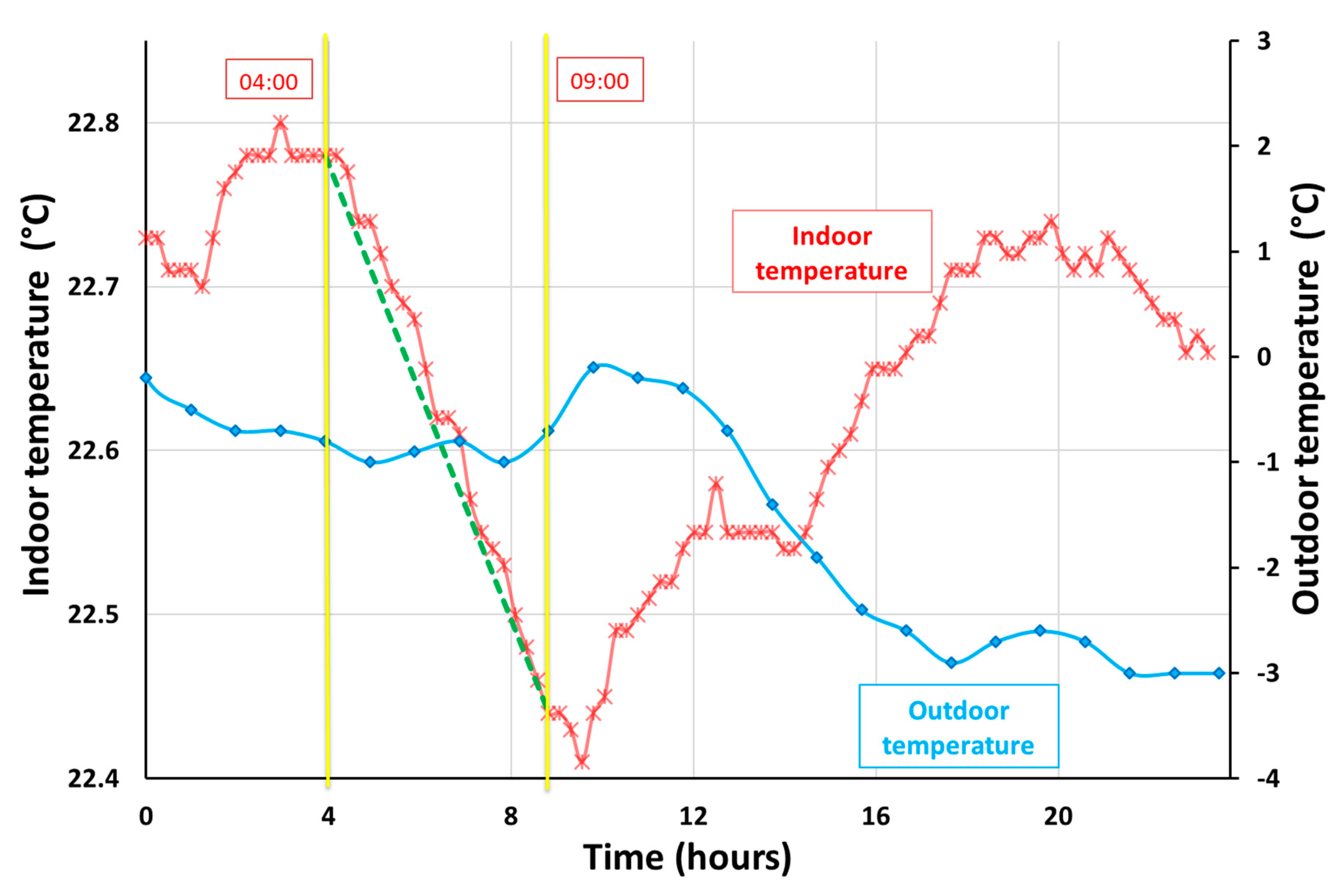
• Indoor temperatures (°C) (hourly averaged value of all the building’s apartments is used in this study). Indoor temperature in each apartment is measured and monitored in one position in the main entrance hall (around 1 m above the floor on the wall).
• Hourly outdoor temperature (°C).

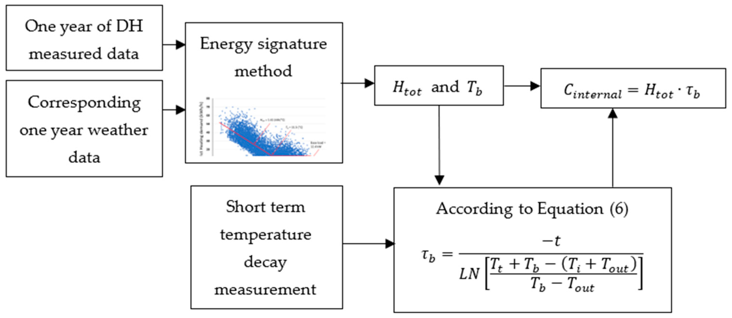
The Calculation Procedure

In order to develop the heat load capacity model, supplied DH and the temperature decay data are used to calculate the building’s time constant. Then, with reference to the outdoor temperature and the supplied DH, H_t + H_v, as well as the balance temperature, T_b, are calculated using the energy signature method on hourly DH data for one year. Lastly, the heat storage capacity is calculated following the steps below and the schematic chart of the procedure is depicted in Figure 2.

• Building time constant

By measuring the indoor temperature decay, the building time constant, τ_b, is calculated considering internal gains, ventilation, and transmission losses, as well as a minor outdoor temperature variation. The temperature drop is caused by the decrease in the DH supply for space heating (however, DH for domestic hot water preparation was still in function).

Equation (3) can be modified to consider heat that is supplied to the building, such as internal heat gains (IHG). If a constant heat power $P_{IHG}$ (or/and partial heat from the heating system) is assumed, then Equation (4) can be derived.

$$T_t=T_{out}+\frac{P_{IHG}}{H_{tot}}+\left(T_i-T_{out}-\frac{P_{IHG}}{H_{tot}}\right)·e^{-\frac{t}{{\tau }_b}} [\text{℃}]$$

(4)

$T_{out}$ is the outdoor temperature, $H_{tot}$ is the total loss coefficient, i.e., summation of the transmission and ventilation loss coefficients, equivalent to H_t + H_v.

The balance temperature of a building, $T_b,$ indicates at which outdoor temperature, or lower, the heating system must supply energy to the building. It is defined according to Equation (5) (here excluding solar gains).

$$T_b=T_i-\frac{P_{IHG}}{H_{tot}}$$

(5)

Equation (4) can be expressed with $T_b$ according to Equation (6):

$$T_t=T_{out}+T_i-T_b+\left(T_b-T_{out}\right)·e^{-\frac{t}{{\tau }_b}}$$

(6)

2.

Total heat loss coefficient and balance temperature

With the supplied DH power and the indoor–outdoor temperature difference, the total heat loss coefficient, including the ventilation and transmission loss coefficients, H_t + H_v, as well as the balance temperature, $T_b$ can be calculated by using the energy signature method. The energy signture is based on depicting the delivered DH power versus the outdoor temperature, which is explained in [41].

3.

Building thermal capacity

With the building time constant, ${\tau }_b$ and the total loss factor, H_tot, the building thermal capacity, C_internal, can be calculated by using Equation (7):

$${\tau }_b=\frac{C_{internal}}{H_{tot}} [s]$$

(7)

4. Results and Discussion

The possibility of temporarily decreasing the supplied DH and consequently the indoor temperature is analyzed and experimented for a multifamily building. The results including the building time are constant, the heat loss coefficient and thermal capacity of the building are presented here.

The results of the energy signature are presented first, since two important parameters, H_tot and T_b, are required for calculating the time constant ${\tau }_b$. Next, results from applying Equation (6) to simulation results with the validated model of [22], show the order of magnitude of a theoretical value on ${\tau }_b$. Finally, field measurement results are presented together with the assessed value for ${\tau }_b$ and energy saving potentials.

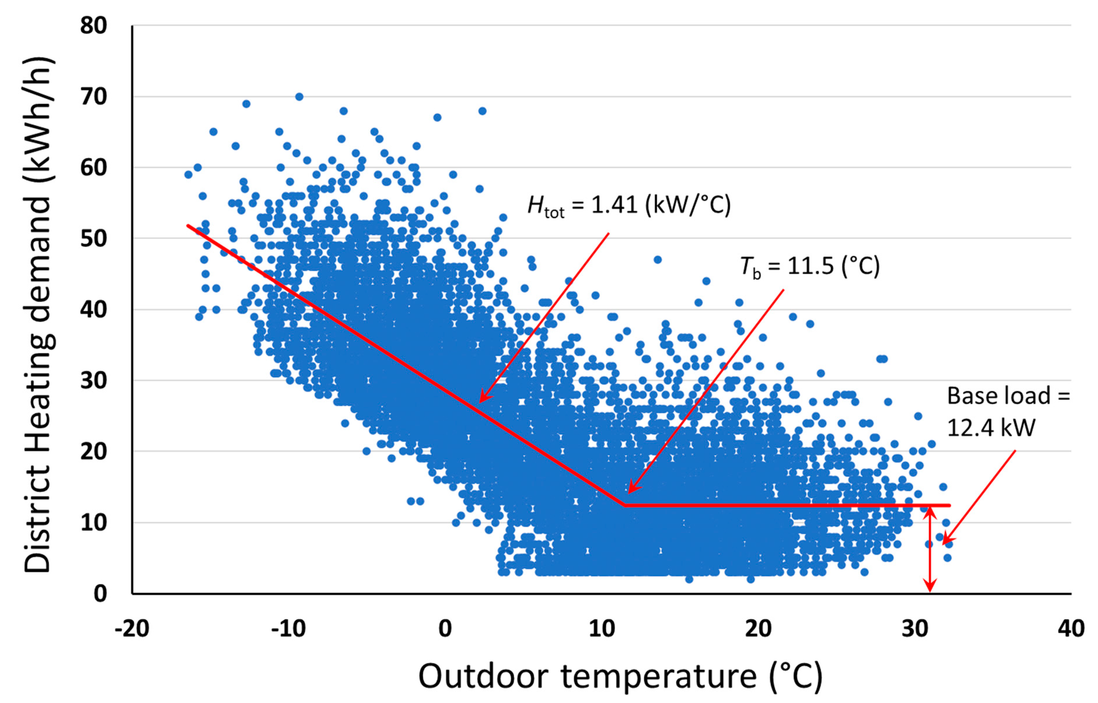
4.1. Building Energy Signature

By Swedish law, supplied DH must be measured with at least a one-hour frequency. This provides data on an annual basis with the possibility of using the data for building analysis purposes. Figure 3 presents the outcomes of applying the energy signature method to the daily values of 2018. Balance temperature, T_b, is considered as 11.5 °C, and the delivered power use for domestic hot water, DHW, is considered as a constant 12.4 kW over the year. The total heat loss coefficient, i.e., the slope in Figure 3, is 1410 W/K.

4.2. Simulated Building Time Constant

The IDA-ICE model was used to test the application of Equation (6). The simulated building was exposed to the weather of 2017, at least a month prior to 21 December at 04:00 h, when the field test was conducted. During the field test, the outdoor temperature was approximately −0.9 °C and the weather file was manipulated to have this outdoor temperature for the rest of the year. Figure 4 illustrates the mean operative temperatures of the apartments; operative temperature is used since the weighted air and construction surfaces represent the thermal state within the building in a better way than air temperature only. IHG gives rise to momentary variations in the decaying indoor temperatures. Equation (6) is applied for two curves, which have two different initial temperatures but the same time constant, to enclose the peaks and valleys of the simulated indoor decaying temperature. In Equation (6), T_b is set to 11.5 °C, which is also the value which the simulated curve converges to. ${\tau }_b$ is estimated to 260 h.

The initial indoor temperature of the upper dashed curve was set to 21.9 °C (the same value as the simulated blue curve) and the lower dashed curve to −0.8 °C lower. During the first 5 h, the dashed curves dropped 0.24 °C, whilst the simulated curve was 0.58 °C, owing to the dynamic effect during the first hour (the latter four hours resulted in 0.2 °C).

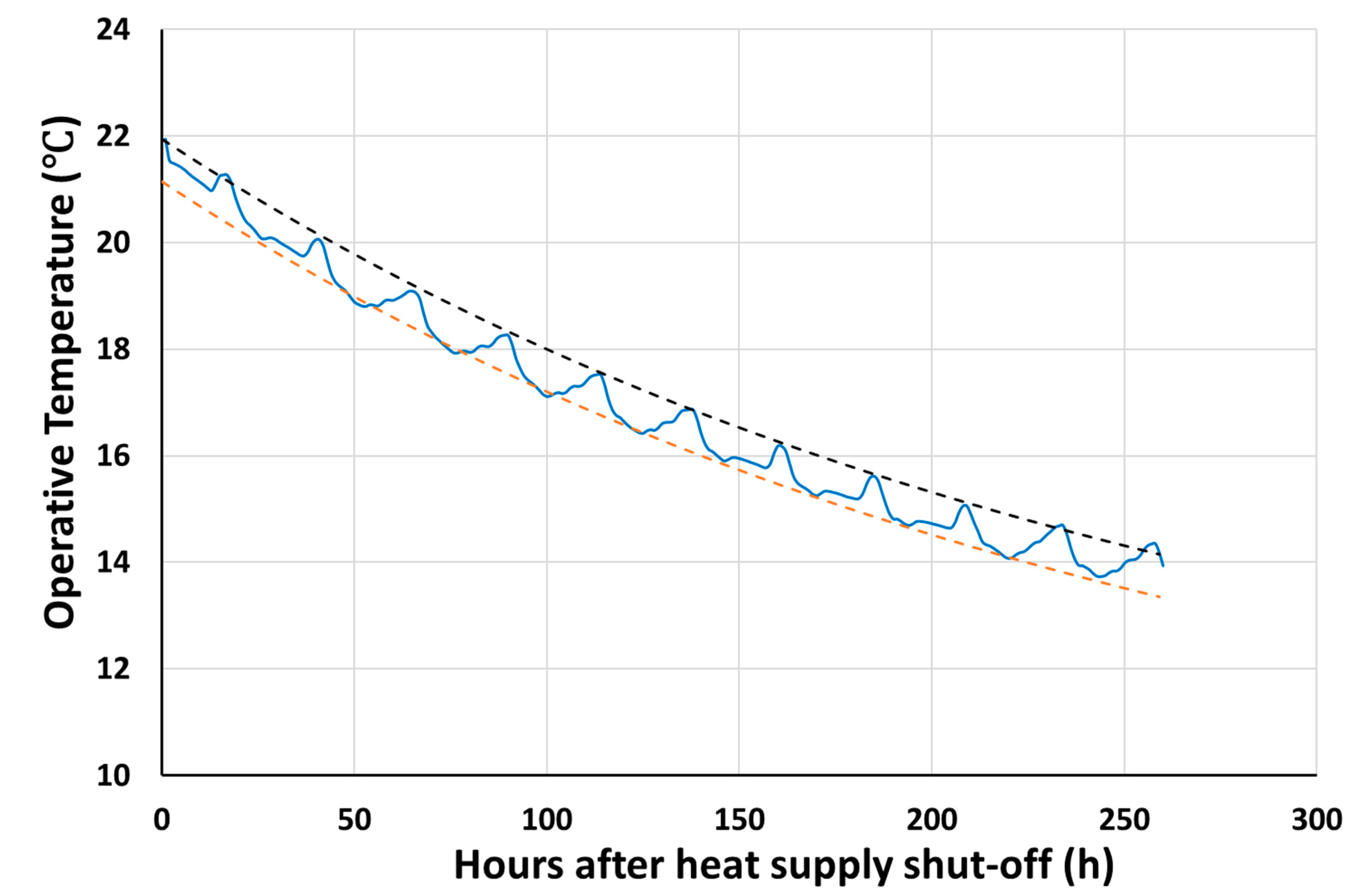
4.3. Field Measurement Building Time Constant

Figure 5 depicts the indoor temperature averaged between the apartments in the studied building, where the decay period is marked with the two yellow vertical lines. The dashed green line in Figure 5 shows an exponential decay curve, calculated by fitting an exponential decay curve to the temperatures at the beginning and end of the decay period. Outdoor temperature is also shown in the figure, which is approximately −0.9 ± 0.1 °C (i.e., with standard deviation of 0.1 °C) during the decay period. The outdoor temperature tends to increase to 0.2 °C at the end of the test period. The temperatures decay due to the decrease in DH supply, and therefore a bottom temperature, at 10:00 is observed right after the decay period, although the DH supply started to increase already at 9:00. This may be due to thermal inertia and a lag in the building heating system, as well as the time it takes for the indoor environment to receive the released heat from the structure and consequently, the indoor temperature is increased. The indoor temperature begins recovering after 10:00, when sufficient DH is supplied to the building and the lack of heating during the decay period is compensated.

The average temperature of the apartments in the building is considered in this study, and if radiators in some apartments are lowered or are out of service, for instance due to not having any tenants, this affects the average temperature of the whole building. The decay period is evident in Figure 5. It is notable that lowering the supplied DH shows an almost direct effect on the indoor air temperature, however, after the decay period, i.e., 09:00, the temperature continues to decrease for the next hour. After that, the indoor temperature starts to increase due to the rise in the DH supply. The average indoor temperature before the decay, shown with red line in Figure 5, is around 22.7 °C, decreasing by 0.3 °C during the test period (5 h). This points to possible further and longer temperature decay in such buildings and consequently less DH supply and peak shaving, without remarkable effects on thermal comfort.

Building time constant from the field measurements, calculated by using Equation (6), gives the value 180 h. This value is lower than that obtained from the simulations. However, there are uncertainties in both values. The time constant is actually not a constant, as pointed out by Kensby et al. [30], since the temperature drop of the indoor air is faster than those of the structures, though these successively converge, as is also shown in [42]. When Equation (6) is used for solving the time constant of the first 5 timesteps after the DH shutdown, the time constant becomes 104 h, much owing to the immediate drop after shutdown (see Figure 4). The value 260 h is due to analyzing the long time lapse: more than 250 h. Moreover, the simulated temperature drop was simulated to be 0.6 °C, which is twice what was measured. This could be due to the modelling of the building; the simulation model does not include furnishing, which can increase the time constant [43] but also reduce the thermal exchange between building structures and air, such as the effect of having carpets, thereby reducing the time constant. Moreover, the apartments were modelled as single zones in which interior walls were lumped as a mass within the zone. Finally, the internal heat gains are modelled according to profiles suggested by Widén et al. [44]. Since the same profile is applied to all apartments, these will have a large impact on temperatures during short shutdown periods and not be identical to that of the actual building. The influence of internal heat gains is reflected in T_b and, as shown in the simulation, is the value that an endlessly long decay would asymptotically converge to. However, T_b is not a constant value [22,45] and does vary over time.

The uncertainty of the field measurement comes from the relatively short measurement period and small temperature drop—which temperature is actually measured? The sensor is mounted on a hall wall in each apartment, probably measuring a weighted value for air and wall temperature, implying that this temperature and the temperature used in the simulations are not entirely comparable. As previously mentioned, air and structure temperature eventually converge but deviate in the initial stages. However, this method, which is based on readily available data that give H_tot and T_b, can, with a short shutdown of space heating supply and registering of indoor temperature decay, give an indication of the order of magnitude of the time constant, corresponding to that of the test decay period. In turn, the time constant is valuable for assessing how long shutdown periods can be, and which temperature decays can, on average, be expected. A benefit is that this type of assessment can be performed at a large scale, such as neighborhood blocks or city districts.

Delivered DH during the decay period is shown in Figure 6, as well as the outdoor temperature. The dashed green line in Figure 6 shows the DH supply considering the straight linear supply between 4:00 and 13:00, i.e., without any peaks or valleys in the DH supply. To estimate the power supply, without the decrease in DH supply, the period between 04:00 and 13:00 is considered to be the corrected supplied DH, including the peak after the decay period. The peak occurs to compensate the cooler period and warm up the interior. The corrected DH supply is considered as the average supply between this period, 04:00 and 13:00, shown by the dashed green line in Figure 6.

The DH power is expressed by kWh/h, which means that the area below the diagram in Figure 6, during a certain period, shows the supplied DH. However, it should be noticed that the supplied power should be studied per hour, because that is what the energy company provides for its customers, and the extreme peaks and variations in the power demand might be challenging and expensive to be supplied. The delivered or supplied DH is presented for the whole period, in which there are hours with very low power demand and hours with very high peaks. Thus, analyzing the DH, both energy and power should be studied. A more even load curve would be more economical and environmentally friendly and would lead to a more reliable and sustainable energy supply. The average hourly supplied DH power to the building, shown by the red line in Figure 6, is 31.5 kWh/h for the whole test day, which decreased to 12.2 kWh/h during the decay period.

Note that at 05:00, inertia in the DH system never reached zero. There are two reasons for this; the DHW circulations have losses, which are compensated by DH (on average 2.9 kW [22]). Moreover, the heating power increases, which is probably due to occupants using DHW. The heating of DHW is not restricted, though the space heating function is off.

4.4. Building Thermal Capacity

The main results are shown in

Table 1. Summary of the results, including indoor temperature and its decay, delivered power, calculated building time constant, and thermal capacity.

Heated Area	Indoor Temperature (Averaged between 4:00–9:00)	Indoor Temperature Decay (4:00–9:00)	Time Constant	Supplied DH Power (Hourly Averaged between 4:00–9:00)	Supplied DH (21 December)	Corrected Supplied DH (21 December)	Saved DH (21 December)	Heat Loss Coefficient	Thermal Capacity
m2	°C	°C	h	kWh/h	kWh	kWh	kWh	W/K	kWh/K
2445	22.6	0.3	180	12.2	755	818	63	1410	253.8

, including the indoor temperature and its decay (during the test period), delivered power/energy and the saved power/energy, heat loss coefficient, building time constant, and thermal capacity of each building. The mean outdoor temperature during the test day, 21 December, was −1.5 ± 1.1 °C, and during the test period, 04:00–9:00, it was −0.9 °C.

The results for the total supplied and saved DH during the test period are shown in Table 1. The DH supplied to the building over the whole test day decreased by 63 kWh, or 8%, when compared with the corrected supplied DH, i.e., in case if the decrease in DH would not be implemented. During the test period, 61 kWh DH was supplied and an estimated 94 kWh or 60.8% heat was saved during the test period, i.e., 4:00–9:00 compared with the corrected heat supply in the same period—see the dashed line in Figure 6. The difference between the reduced DH supply, i.e., 63 kWh during the whole test day and the 94 kWh during the test period of 4:00–9:00, is that, although the peak loads in the delivered DH were reduced during the decay period, some peak load were observed right after the decay period to compensate for the lack of heat supply during the test period. According to the results shown in 5, the average hourly supplied DH power to the building, 31.5 kWh/h for the whole test day, was decreased to 12.2 kWh/h during the decay period. Due to the reduction in DH supply, some peaks were avoided, however, it is challenging to calculate the exact reduction in peak power during the decay period. Comparing with the corrected heat supply (see the dashed line in Figure 6), it is estimated that the supplied DH power averaged over the whole test day, i.e., 31.5 kWh/h, was decreased by 8%. Thermal capacity of the studied multifamily building is also calculated using Equation (7), as 253.8 kWh/K.

The outdoor temperature, see Figure 5, slightly increased after the decay period, and consequently the indoor–outdoor temperature difference decreased, which compensated for the lack of DH supply during the test period. Thus, the proposed test led to a small saving, 3 kWh, in the supplied DH, in comparison with the corrected DH supply. The reason for this may be due to the high building time constant and thermal capacity of the building, as well as the indoor air that compensates for the lack of DH supply and maintains the indoor temperature. This may also be due to the interaction of occupants, for instance, increasing the setpoint temperatures of the hydronic radiators in each apartment or increasing the use of domestic hot water, e.g., by taking a shower, and in that case, receiving more DH into their apartments.

There are different resources that can be used to produce and supply heat in a DH network, and depending on the source, the production costs can vary greatly. It should be noticed that supplying the higher peak demands in a DH network is often engaged with more GHG emissions and up to 10 times more expensive resources. Moreover, some energy companies even charge their customers based on the power they are subscribed to, and exceeding that power might lead to extra charges. The annual DH supply for the building is approximately 184 MWh, and the exact economical saving of the energy storage can be calculated based on the time and order in which different resources are used.

The amount of saving per each decay occasion is not significant, but frequent similar decays can be accomplished throughout the year without compromising inhabitants’ thermal comfort, and the stored heat in the building structure can be used and released in order to save energy and power during the peak periods. Moreover, a similar procedure can be used by connecting further buildings, blocks, and districts; therefore, more saving can be achieved both in the peak loads as well as in the economical savings for both the customers and the energy company. The benefits are even greater for the energy company, as they can better manage and plan their production with more environmentally friendly and cheaper resources. Likewise, when there is maintenance in the DH network, eventual temporary reduction in the DH supply can be managed and planned based on the thermal storage and heat capacity of the connected building structures, as the proposed example in the current study.

More than saving the cost of the production, CO₂ emissions depend on the energy sources being used in DH production. During the peak hours, often sources such as fossil fuels, with higher CO₂ emissions, are used, as well as other combustion-related contaminants. Thus, decreasing the higher loads in the peak demand hours will also lead to a decrease in CO₂ emissions. This is even more important than the economic profit of peak load management for reaching the climate goal of keeping the global temperature increase within 1.5 °C, compared to pre-industrial levels.

Building time constant is often calculated based on a temperature drop in the indoor temperature due to a reduction in supplied energy. The outdoor temperature was assumed constant during the decay period (5 h), and the average outdoor temperature was considered in the calculation, as the variations were negligible. Moreover, the internal heat gains from inhabitants, household appliances, lighting, equipment, and possible solar irradiation were also considered, i.e., all the gains in real life scenario. Thus, the calculated time constant is more representative of the thermal storage capacity of the whole building block.

The studied multifamily building has several apartments/flats, and the average temperature (between the apartments) is used in this study, as the DH supply is steered for the whole building, not on the basis of each flat. In addition, the apartments might have different thermal properties, such as U-value and airtightness, and therefore respond differently to the DH variations. This will limit the control strategy, perhaps, to the apartments that have the largest indoor temperature drop during the decay periods, because the aim is not to compromise the thermal comfort. If the DH supply could be steered separately to each apartment of a building, then more specific and separate control strategies could be allocated based on each apartment. This would lead to achieving the maximum amount of power and energy saving by maximizing the temperature and DH decay in each apartment unit while having all indoor temperatures within the acceptable thermal comfort range. Thus, a more detailed control system installed in each apartment is suggested to enhance the model accuracy and increase its saving potential. The other decisive factors include the user related parameters, for instance, airing (opening of balcony doors or windows) and the occupancy schedule. Implementing such user-related parameters can increase the model performance and saving potential, however, the accurate monitoring or simulations of, for instance, airing or the occupancy schedule, can be challenging, and these parameters are already included indirectly in the calculation procedure, as they affect the indoor temperature and heat supply, respectively.

Based on the heat storage capacity of the connected building, a load management schedule can be provided for DH networks in order to temporarily store the DH and mitigate the peak loads. The significance of the load management will be clearer if more buildings are connected to the DH network, and therefore, having a more uniform DH supply would be more challenging and important. Furthermore, buildings can be categorized based on their thermal inertia and storage capacity, i.e., their time constants, and separate load management strategies can be suggested using, for instance, machine learning algorithms that can be adjusted based on weather predictions and occupancy behavior/schedule. The energy (or power) signature diagram (i.e., annual delivered DH energy or power to the buildings) can be modified by considering the thermal storage capacity within the buildings, i.e., the maximum capacity of the building to temporarily store DH and mitigate the peak power loads in the network.

Further analysis, to find a practice routine governing the supplied DH based on each apartment’s temperature and optimizing the decay period resulting in lower peaks, is suggested for future studies. Furthermore, the method can be applied to monitor the heating supply of other building types. A heat storage and control model can be developed with the help of artificial intelligence (AI), finding the relationship between DH supply and demand patterns. The AI model can learn from the input data and predict the delivered DH power based on the outdoor temperature prediction, absorbed solar gain, occupant schedule (say during the next 24 h or coming week), and expected indoor temperature.

5. Conclusions

The heat storage capacity of a multifamily building, connected to a district heating network, is calculated in this paper by reducing the DH supply temporarily, and the resulting indoor temperature decays. The proposed method can be used in other types of buildings, and the building structure can be used as a thermal battery to store thermal energy in advance to be used during the peak demand hours, e.g., in case of the encountering of a colder climate. The DH supply to the building was reduced during 5 h during the test day, which was 21 December 2017. The supplied DH to the building through the test day was 755 kWh. The results show that in total, 63 kWh, or 8% DH, could be saved in the connected building.

Moreover, during the decay period, 04:00–09:00, the total supplied DH was 61 kWh, which is estimated to have a 60.8% decrease in the hourly supplied DH to the building. This was compensated by the produced peak after the decay period, and the supplied DH power averaged over the whole test day, i.e., 31.5 kWh/h, was estimated to be decreased by 8%.

Implementing a similar method of using building structures as thermal batteries in order to reduce the peak loads can lead to considerable saving in the supplied DH throughout the year. The method would also be useful for network maintenance or for the expansion of the network, where the DH supply capacity would be temporarily limited and therefore more sensitive to the peak demands. The economic gain of the DH supply control and the reduction of it temporarily depends on the resources used in the production plants. DH can be stored in the structures, prior to maintenance and operational interruptions in the networks or in occasions prior to upcoming peak loads based on weather prognoses, to insure the reliable and continuous DH delivery and gain more customer satisfaction. As often more expensive and less environmentally friendly sources are used to fulfill the DH supply in the peak demand period, the proposed method of storing DH can lead to a more sustainable and environmentally friendly DH network. The saved energy/power can also lead to economic savings for the connected customers, as higher tariffs due to extra peak loads can be avoided.

In addition, more tests involving larger temperature decay and longer duration can be performed to find the optimum threshold and maximum heat storage capacity of the network. Such tests are non-intrusive and can be controlled centrally by the energy company via the DH distribution central units. The next step after mapping the heat storage capacity is to map the peak demands of the DH supply network, including their frequency and duration. Other parameters, such as available DH sources, possible maintenance or expansion of the network, and also the schedule for the occupancy and DH use within the building structure can be considered as well.

References

1. Cui, Y.; Yan, D.; Hong, T.; Xiao, C.; Luo, X.; Zhang, Q. Comparison of typical year and multiyear building simulations using a 55-year actual weather data set from China. Appl. Energy 2017, 195, 890–904. [Google Scholar] [CrossRef] [Green Version]
2. Abergel, T.; Dean, B.; Dulac, J.; Hamilton, I. Status Report Towards a Zero-Emission, Efficient and Resilient Buildings and Construction Sector; Global Alliance for Buildings and Construction: Paris, France, 2018. [Google Scholar]
3. United Nations United Nations Sustainable Development Goals (SDGs). Available online: https://sdgs.un.org/goals (accessed on 6 July 2022).
4. Campaniço, H.; Soares, P.M.M.; Cardoso, R.M.; Hollmuller, P. Impact of climate change on building cooling potential of direct ventilation and evaporative cooling: A high resolution view for the Iberian Peninsula. Energy Build. 2019, 192, 31–44. [Google Scholar] [CrossRef]
5. European Commission. Climate Action: European Climate Law. Available online: https://ec.europa.eu/clima/eu-action/european-green-deal/european-climate-law_en (accessed on 6 July 2022).
6. European Commission. A European Green Deal: Striving to be the First Climate-Neutral Continent. Available online: https://ec.europa.eu/info/strategy/priorities-2019-2024/european-green-deal_en (accessed on 6 July 2022).
7. Energiföretagen Miljövärdering av Fjärrvärme [Report in Swedish: Environmental Assessment of District Heating]. Available online: https://www.energiforetagen.se/statistik/fjarrvarmestatistik/miljovardering-av-fjarrvarme/ (accessed on 15 December 2021).
8. Frederksen, S.; Werner, S. District Heating and Cooling; Studentlitteratur AB: Lund, Sweden, 2013; ISBN 978-9-14408-530-2. [Google Scholar]
9. Energimarknadsbyrån Vad är Fjärrvärme? Available online: https://www.energimarknadsbyran.se/fjarrvarme/vad-ar-fjarrvarme/ (accessed on 15 December 2021).
10. Noussan, M.; Jarre, M.; Poggio, A. Real Operation Data Analysis on District Heating Load Patterns. Energy 2017, 129, 70–78. [Google Scholar] [CrossRef] [Green Version]
11. Lund, H.; Østergaard, P.A.; Chang, M.; Werner, S.; Svendsen, S.; Sorknæs, P.; Thorsen, J.E.; Hvelplund, F.; Mortensen, B.O.G.; Mathiesen, B.V.; et al. The status of 4th generation district heating: Research and results. Energy 2018, 164, 147–159. [Google Scholar] [CrossRef]
12. Lund, H.; Werner, S.; Wiltshire, R.; Svendsen, S.; Thorsen, J.E.; Hvelplund, F.; Mathiesen, B.V. 4th Generation District Heating (4GDH): Integrating smart thermal grids into future sustainable energy systems. Energy 2014, 68, 1–11. [Google Scholar] [CrossRef]
13. Persson, U.; Werner, S. Heat distribution and the future competitiveness of district heating. Appl. Energy 2011, 88, 568–576. [Google Scholar] [CrossRef]
14. Gadd, H.; Werner, S. Achieving low return temperatures from district heating substations. Appl. Energy 2014, 136, 59–67. [Google Scholar] [CrossRef] [Green Version]
15. Verda, V.; Colella, F. Primary energy savings through thermal storage in district heating networks. Energy 2011, 36, 4278–4286. [Google Scholar] [CrossRef]
16. Vandermeulen, A.; van der Heijde, B.; Helsen, L. Controlling district heating and cooling networks to unlock flexibility: A review. Energy 2018, 151, 103–115. [Google Scholar] [CrossRef]
17. Werner, S. The Heat Load in District Heating Systems. Ph.D. Thesis, Chalmers University of Technology, Chalmers, Sweden, 1984. [Google Scholar]
18. Gadd, H.; Werner, S. Daily heat load variations in Swedish district heating systems. Appl. Energy 2013, 106, 47–55. [Google Scholar] [CrossRef] [Green Version]
19. Gadd, H.; Werner, S. Heat load patterns in district heating substations. Appl. Energy 2013, 108, 176–183. [Google Scholar] [CrossRef] [Green Version]
20. Calikus, E.; Nowaczyk, S.; Sant’Anna, A.; Gadd, H.; Werner, S. A data-driven approach for discovering heat load patterns in district heating. Appl. Energy 2019, 252, 113409. [Google Scholar] [CrossRef]
21. Buffa, S.; Fouladfar, M.H.; Franchini, G.; Lozano Gabarre, I.; Andrés Chicote, M. Advanced Control and Fault Detection Strategies for District Heating and Cooling Systems—A Review. Appl. Sci. 2021, 11, 455. [Google Scholar] [CrossRef]
22. Eriksson, M.; Akander, J.; Moshfegh, B. Development and validation of energy signature method—Case study on a multi-family building in Sweden before and after deep renovation. Energy Build. 2020, 210, 109756. [Google Scholar] [CrossRef]
23. Nordström, G.; Johnsson, H.; Lidelöw, S. Using the energy signature method to estimate the effective U-value of buildings. In Sustainability in Energy and Buildings; Springer: Berlin/Heidelberg, Germany, 2013; pp. 35–44. [Google Scholar]
24. Arteconi, A.; Costola, D.; Hoes, P.; Hensen, J.L.M. Analysis of control strategies for thermally activated building systems under demand side management mechanisms. Energy Build. 2014, 80, 384–393. [Google Scholar] [CrossRef] [Green Version]
25. Johansson, C.; Wernstedt, F.; Davidsson, P. Distributed thermal storage using multi-agent systems. In Proceedings of the International Conference on Agreement Technologies, Dubrovnik, Croatia, 15–16 October 2012. [Google Scholar]
26. Mathiesen, B.V.; Drysdale, D.; Lund, H.; Paardekooper, S.; Ridjan, I.; Connolly, D.; Thellufsen, J.Z.; Jensen, J.S. Future Green Buildings: A Key to Cost-Effective Sustainable Energy Systems; Aalborg University: Aalborg, Denmark, 2016. [Google Scholar]
27. Turski, M.; Sekret, R. Buildings and a district heating network as thermal energy storages in the district heating system. Energy Build. 2018, 179, 49–56. [Google Scholar] [CrossRef]
28. Masy, G.; Georges, E.; Verhelst, C.; Lemort, V.; André, P. Smart grid energy flexible buildings through the use of heat pumps and building thermal mass as energy storage in the Belgian context. Sci. Technol. Built Environ. 2015, 21, 800–811. [Google Scholar] [CrossRef]
29. Reynders, G. Quantifying the Impact of Building Design on the Potential of Structural Storage for Active Demand Response in Residential Buildings. Ph.D. Thesis, KU Leuven, Leuven, Belgium, 2015. [Google Scholar]
30. Kensby, J.; Trüschel, A.; Dalenbäck, J.-O. Potential of residential buildings as thermal energy storage in district heating systems—Results from a pilot test. Appl. Energy 2015, 137, 773–781. [Google Scholar] [CrossRef]
31. Cholewa, T.; Siuta-Olcha, A.; Smolarz, A.; Muryjas, P.; Wolszczak, P.; Guz, Ł.; Bocian, M.; Balaras, C.A. An easy and widely applicable forecast control for heating systems in existing and new buildings: First field experiences. J. Clean. Prod. 2022, 352, 131605. [Google Scholar] [CrossRef]
32. Bilous, I.; Deshko, V.; Sukhodub, I. Parametric analysis of external and internal factors influence on building energy performance using non-linear multivariate regression models. J. Build. Eng. 2018, 20, 327–336. [Google Scholar] [CrossRef]
33. Gadd, H.; Werner, S. Fault detection in district heating substations. Appl. Energy 2015, 157, 51–59. [Google Scholar] [CrossRef] [Green Version]
34. Abel, E.; Nilsson, P.-E.; Ekberg, L.; Fahlén, P.; Jagemar, L.; Clark, R.; Fanger, O.; Fitzner, K.; Gunnarsen, L.; Nielsen, P.V. Achieving the Desired Indoor Climate-Energy Efficiency Aspects of System Design; Studentlitteratur: Skåne Län, Sweden, 2003; ISBN 9-14-40323-58. [Google Scholar]
35. Boverket Öppna Data—Dimensionerande Vinterutetemperatur (DVUT 1981-2010) för 310 Orter i Sverige. Available online: https://www.boverket.se/contentassets/b6c74238383c4b4e82b6d0c7311a1534/smhi-210976-v1-smhi_rapport_2016_69_dimensionerande_vinterutetemperatur_dvut_1981-2010_310_orter.pdf (accessed on 16 December 2021).
36. BS EN ISO 52016-1:2017; Energy Performance of Buildings—Energy Needs for Heating and Cooling, Internal Temperatures and Sensible and Latent Heat Loads—Part 1: Calculation Procedures. ISO: Geneva, Switzerland, 2017.
37. EQUA AB IDA Indoor Climate and Energy. Available online: http://www.equa.se/en/ida-ice (accessed on 1 August 2017).
38. Kropf, S.; Zweifel, G. Validation of the Building Simulation Program IDA-ICE According to CEN 13791 “Thermal Performance of Buildings-Calculation of Internal Temperatures of a Room in Summer Without Mechanical Cooling-General Criteria and Validation Procedures”; HLK Engineering: New Delhi, India, 2001. [Google Scholar]
39. Moosberger, S. IDA ICE CIBSE-Validation: Test of IDA Indoor Climate and Energy Version 4.0 According to CIBSE TM33, Issue 3; EQAU Simulation Technology Group: Stockholm, Sweden, 2007. [Google Scholar]
40. Hayati, A. Measurements and modeling of airing through porches of a historical church. Sci. Technol. Built Environ. 2018, 24, 270–280. [Google Scholar] [CrossRef] [Green Version]
41. Eriksson, M. A Statistical Approach to Estimate Thermal Performance and Energy Renovation of Multifamily Buildings: Case Study on a Swedish City District. Licentiate dissertation. Gävle University: Gävle, Sweden, 2022. [Google Scholar]
42. Erba, S.; Barbieri, A. Retrofitting buildings into thermal batteries for demand-side flexibility and thermal safety during power outages in winter. Energies 2022, 15, 4405. [Google Scholar] [CrossRef]
43. Johra, H.; Heiselberg, P.; Le Dréau, J. Influence of envelope, structural thermal mass and indoor content on the building heating energy flexibility. Energy Build. 2019, 183, 15. [Google Scholar] [CrossRef]
44. Widén, J.; Lundh, M.; Vassileva, I.; Dahlquist, E.; Ellegård, K.; Wäckelgård, E. Constructing load profiles for household electricity and hot water from time-use da-ta-modelling approach and validation. Energy Build. 2017, 41, 753–768. [Google Scholar] [CrossRef]
45. Rasmussen, C.; Bacher, P.; Calì, D.; Nielsen, H.A.; Madsen, H. Method for scalable and automatised thermal building performance documentation and screening. Energies 2020, 13, 3866. [Google Scholar] [CrossRef]
Figure 1. The simulated multifamily building, (a) real building (left), and (b) the IDA-ICE simulation model (right).
Buildings 12 01007 g001
Figure 2. The schematic chart of the calculation procedure for the proposed heat load capacity model.
Buildings 12 01007 g002
Figure 3. Energy signature diagram for the supplied district heating for space and DHW heating of the studied multifamily building. The blue points represent the daily average supplied DH in 2018.
Buildings 12 01007 g003
Figure 4. Temperature decay from simulations after DH shut-off. IHG causes variations in temperature, but decay is steadily arriving at approximately Tb = 11.5 °C. Dashed lines are modelled with Equation (6), with τ b estimated to 260 h.
Buildings 12 01007 g004
Figure 5. Indoor temperature for the studied building both before and during the temperature decay.
Buildings 12 01007 g005
Figure 6. Delivered district heating (DH) power for the building and the outdoor temperature both before and during the temperature decay.
Buildings 12 01007 g006