1. Introduction
In recent years, there has been a special focus on reducing energy consumption, particularly in buildings. For example, in the European Union it is estimated that buildings are accountable for more than 40% of energy consumption [
1]. In this perspective, researchers have been studying the contribution to energy consumption by the building envelopes, where the respective facades are the most significant element. The facades allow the protection of the interior spaces and the regulation of the interactions between the exterior and interior environments. Currently, more and more buildings resort to the use of facades with large areas of glazed surfaces, which cause some problems such as thermal discomfort, low acoustic insulation, poor natural ventilation, and increased energy consumption [
2,
3]. Thus, in the search for solutions to these problems, new facade technologies have been developed and applied. Among these new advanced technologies, a Double Skin Facade (DSF) stands out as an efficient solution in regulating interactions between interior and exterior environments [
4,
5,
6].
A DSF is basically constituted of “an external glazed skin and the actual building facade, which constitutes the inner skin, where the two layers are separated by an air cavity, which has fixed or controllable inlets and outlets and may or may not incorporate fixed or controllable shading devices” [
7]. The shading devices inserted in this air cavity are usually a Venetian-type blind. In this air cavity, it is also possible to install energy-saving devices such as photovoltaic cells, with, for example, significant heating energy gains in winter conditions [
8]. The air ventilation in the cavity can be controlled using natural, hybrid (fan supported) or mechanical ventilation strategies [
9]. The technical features of the DSF lean on the facade typology, skin coverage, air ventilation strategies, shading device integration, building use and location, among others [
10].
Several studies on the most varied aspects of DSF construction, use and performance have been carried out in recent years. The benefits and economic feasibility obtained by the use of DSF are presented in detail in the study of Ghaffarianhoseini et al. [
9]. DSF technical aspects and its impact on building energy efficiency, thermal behavior and daylighting performance are also analyzed in this study [
9]. According to the review study of Lucchino et al. [
11], it is important to use building energy simulation tools to simulate the performance of the DSF before its implementation in buildings. As an example, see the numerical study of Xue and Li [
12], where a DSF naturally ventilated optimal design and thermal behavior analysis was carried out by a new fast and accurate computational fluid dynamics model.
Protection from direct solar radiation and against sound transmission can be obtained using DSF with integrated shading devices [
13,
14]. The DSF cavity air temperature, air velocity and airflow behavior are affected by the blinds geometry, which in turn will influence the DSF performance referring to thermal and energy savings [
14,
15]. The blinds geometry depends on air cavity dimensions, orientation, and material properties (reflection, absorbance and transmission). The use of materials such as dielectric film coatings or pastel paints [
16], and phase change material integrated in the blinds [
17], can improve the thermal performance of DSF.
Currently, it is important to have well-designed Heating, Ventilation Air Conditioning (HVAC) systems installed in buildings in order to simultaneously ensure acceptable levels of thermal comfort and indoor air quality for a significant percentage of occupants. The level of thermal comfort can be evaluated by PMV (Predicted Mean Vote) and PPD (Predicted Percentage of Dissatisfied) indexes, developed by Fanger [
18], and used by the international standards ISO 7730 [
19] and ASHRAE Standard 55 [
20]. The indoor air quality level can be evaluated by the carbon dioxide (CO
2) concentration values. In this case, the ASHRAE Standard 62.1 [
21] can be used to assess the indoor air quality level.
This study implements a ventilation system founded on ceiling-mounted, localized air distribution systems, which are based on vertical descendent jets. This kind of ventilation system is characterized by providing clean outside air directly to the body sections or breathing area of occupants at low air velocity and air turbulence intensity. It also allows occupants to control air temperature, airflow rate and airflow direction [
22].
Some numerical and experimental works have been developed on this subject [
22,
23,
24,
25]. Conceição et al. [
22] numerically compared the performance of four different ceiling-mounted, localized air distribution ventilation systems using vertical descending jets placed above the occupants in a virtual classroom in order to optimize their positions inside the experimental classroom. These systems have two different air supply temperatures and the virtual classroom has two types of occupancy. Yang et al. conducted several experiments for different ceiling-mounted, localized air distribution ventilation systems using different room air temperatures, air supply temperatures and airflow rates combinations in order to analyze the influence of these systems on the plume of a seated thermal manikin [
23]. In the experimental work of Yang et al. [
24], in a hot humid climate, they obtained energy savings with the use of this type of ventilation system relative to a mixed ventilation system. In the numerical and experimental work conducted by Makhoul et al. [
25], they used a ceiling-mounted, localized air distribution ventilation system and small desk fan to control the thermal plumes around occupants. This kind of system was able to improve the performance of the single jet personalized ventilation nozzles and to reduce energy consumption when compared with the usual mixing ventilation systems.
The study of Yang et al. [
26] presented a new ceiling-mounted personalized system, the performance of which was evaluated in an experimental environmental chamber for four different airflow rates. This system allowed them to obtain an improvement of thermal comfort and indoor air quality when the personalized ventilation airflow rates were increased. The performance of another new ceiling-mounted personalized ventilation system was numerically optimized using computational fluid dynamic simulations [
27]. The optimization focused on determining the airflow rate for the best combination of thermal comfort and indoor air quality [
27]. The model used was validated experimentally utilizing a thermal manikin inside an experimental environmental chamber. The experimental study conducted by Nielsen et al. [
28] demonstrated that the performance of ceiling-mounted air distribution ventilation systems compared to the air distribution obtained by mixing ventilation, vertical ventilation, and displacement ventilation, presented better thermal conditions and fewer local discomfort conditions. The numerical work of Haghshenaskashani and Sajadi [
29] showed that the location of the exhaust ventilation system has an impact on the improvement of the indoor thermal comfort and the energy consumption of the used impinging jet ventilation system. This study also demonstrated that the exhaust ventilation system must be located higher than 1.8 m and that its location on the ceiling is a good option.
The influence of the ceiling-mounted, localized air distribution ventilation system on the occupant thermal comfort and air quality is evaluated by the Air Diffusion Index (ADI). The ADI allows establishing a criterion for assessing the performance of ventilation systems [
30], simultaneously considering air quality, Fanger [
31], and thermal comfort, ISO 7730 [
19] concepts. This index was presented in detail for uniform environments in Awbi [
30] and for non-uniform environments in Conceição et al. [
32]. It was applied, for example, in the work of Karimipanah et al. [
33].
In this work some novelties are proposed, both in terms of innovations introduced in the ventilation system used, and in the numerical simulation methodology implemented. With regard to construction aspects, a new solution is proposed in which thermal energy is produced in DSF and transported to an upper duct where a descendent jet ventilation strategy is applied. This new ventilation system consists of an insufflation system and an extraction system. The air insufflation system in the compartment consists of descending jets that are located above the occupants’ heads, whose associated thermal energy is produced throughout the day in a south-facing DSF. The new proposed extraction system consists of several vertical ducts placed in the longitudinal direction and equally spaced in the center of the compartment. The application of this system is carried out in a chamber that simulates a classroom.
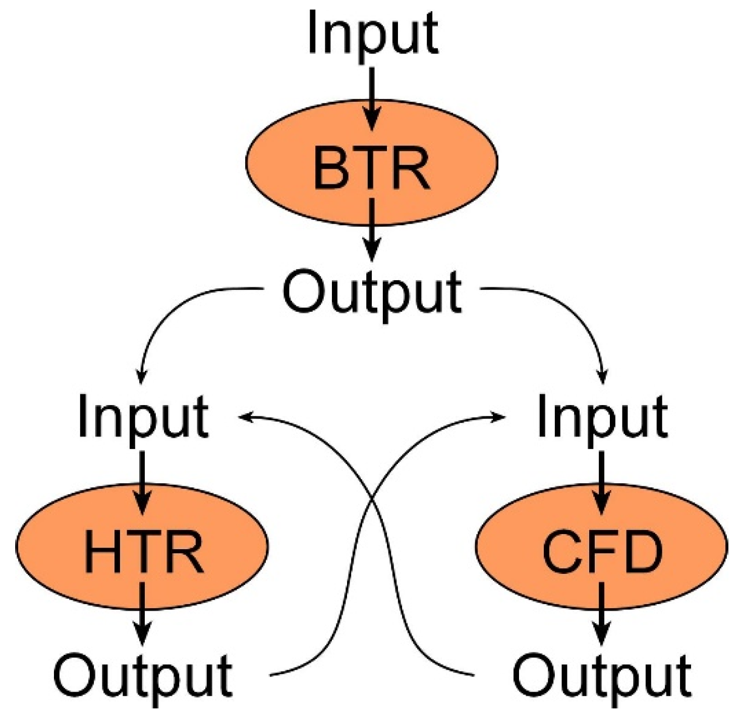
The numerical simulation uses three pieces of research software, developed for this purpose: one to simulate the building thermal response (BTR), one for a coupling between a human thermal-physiology response (HTR) and the other using computational fluid dynamics (CFD). The BTR simulates the thermal behavior of the building, under transient conditions, throughout the day. This software includes models referring to solar radiation, from the extraterrestrial component to the surfaces with arbitrary inclination in the building, the thermal response of buildings, the flow inside, considering water vapor and carbon monoxide, and the transfer of information to coupled software, among others. The thermal response models consider conduction and convection in all layers of opaque and transparent surfaces, radiation transmission on building surfaces, from absorption and reflection on all surfaces, to transmission on transparent surfaces and considering all existing shading. CFD calculates the flow within the occupied space, especially the flow around people. The HTR simulates the thermal response of people and clothing, the thermoregulatory system, the circulatory system, and assesses the level of thermal comfort, taking into account heat fluxes and PMV index, among others.
The purpose of this work is to numerically analyze the contribution of renewable solar energy production in a DSF system and its application in a new HVAC system based on ceiling-mounted localized air distribution systems to the improvement of the occupants’ thermal comfort and indoor air quality. In addition, in this work, which simulates a real situation, we also propose to analyze in detail both the levels of thermal comfort and indoor air quality (IAQ) provided by this ventilation system, to which each occupant is subject, also considering the energy produced in the DSF system.
2. Numerical Model and Methodology
2.1. Numerical Model
This numerical work considers a virtual classroom, an inlet ceiling-mounted localized air distribution system, an exhaust ventilation system and a DSF system. Each DSF has an internal Venetian-type blind system. The performance of this virtual constructive model, similar to a real one in a laboratory, will be evaluated by research software developed by the authors.
This numerical model considers the BTR model and the coupling of CFD and HTR models (see
Figure 1). The three numerical models, working in a coupling methodology, evaluate the thermal comfort level that the virtual classroom occupants are subjected to and the indoor air quality that the occupants are subjected to in the breathing area.
The BTR numerical model, that works in transient conditions, is based on first order integral energy and mass balance equations (please see, as an example, the works of Conceição and Lúcio [
34] and Conceição et al. [
35]). The first order integral energy balance equations are used to evaluate the air temperature inside the spaces (classroom and three DSF), temperature in the Venetian-type blind, temperature in the transparent glasses, temperature in the opaque bodies and temperature in the interior bodies. These equations consider the convection, conduction evaporation and radiation phenomena. The heat transfer by convection phenomena is calculated by natural, forced and mixed convection, through the use of dimensionless coefficients. In the radiative phenomena, the heat exchanges by radiation, incident solar radiation, solar radiation absorbed by glass, and solar radiation transmitted through the glass are considered. The first order integral mass balance equations are used to evaluate the mass of contaminants (as carbon dioxide concentration) and water vapor. These equations consider the convection and the diffusion phenomena. In the resolution of all equations, the system uses the Runge–Kutta–Fehlberg Method with error control.
In
Figure 1, the input data of the BTR model are as follows:
The building geometry (opaque, transparent and interior bodies) introduced using a Computer-Aided Design methodology;
Geographical location of the building (longitude and latitude);
Outdoor environmental parameters, namely, air temperature, air relative humidity, wind direction and velocity;
Outdoor CO2 concentration;
Occupation and ventilation cycles;
Personal parameters of the occupants (clothing insulation and activity levels);
Other parameters.
The BTR output data, used as input data in the HTR and CFD models (
Figure 1), are the air temperature inside the spaces (classroom and DSF), temperatures in the Venetian-type blinds, transparent glass, opaque and interior bodies, and the mass of contaminants (as CO
2 concentration) and water vapor. The BTR has other output data, namely:
Solar radiation evolution;
Radiation heat exchange;
Convection coefficients;
Indoor air temperature and air velocity;
Indoor CO2 concentration;
PMV and PPD thermal comfort indexes;
Other parameters.
The HTR and CFD numerical models work in a coupling methodology. Coupling techniques were developed and applied in the works of Gau et al. [
36], Almesri et al. [
37], and Conceição et al. [
38].
The HTR numerical model, which works in transient and steady-state conditions and simulates a group of people located inside a space, is based on a first order integral energy and mass balance equation (please, see details in the work of Conceição and Lúcio [
39]). The first order integral energy balance equations, in the human body and clothing thermal system, are used to calculate the temperature of the tissue, the temperature of the arterial and venous blood and the temperature of the clothing. These equations consider the convection, conduction evaporation, and radiation phenomena. The heat transfer by convection phenomena is calculated by natural, forced, and mixed convection, through the use of dimensionless coefficients. In the radiative phenomena, the heat exchanges by radiation and the incident solar radiation are considered. The first order integral mass balance equations are used to calculate the mass of water vapor in the skin surface and in the clothing. These equations consider the convection and the diffusion phenomena. The resolution of all equation systems is also done using the Runge–Kutta–Fehlberg method with error control. This numerical model considers the sub-models of the thermoregulatory system and thermal comfort system.
The input data of the HTR are the air velocity and air temperature around the human body sections, calculated by the CFD, and the Mean Radiant Temperature (MRT). MRT is based on the view factors (calculated through the room and occupant’s geometry) and the surrounding temperatures (room and occupants). The room geometry and temperature field are calculated by the BTR. The air relative humidity is also calculated by the BTR.
The output data of the HTR, used as input in the CFD to assess the human thermal variables, are the temperature in the tissues and temperature of the clothing. The HTR also calculated the thermal comfort level, based on the PPD and PMV indexes.
The CFD numerical model, which works in steady-state conditions and simulates the isothermal and non-isothermal thermal conditions, is based on a second order differential balance equation system (please, see details in the work of Conceição et al. [
40]), constituted of:
The differential Navier–Stokes balance equations, which are used to evaluate the three directional components of air velocity;
The differential energy balance equations, which are used to evaluate the air temperature;
The differential mass balance equations, which are used to evaluate the CO2 concentration;
The differential RNG turbulence model balance equations, which are used to evaluate the turbulent kinetic energy and turbulent energy dissipation.
CFD also has the following features:
Use of the Tridiagonal Matrix Algorithm (TDMA) method to solve all systems of equations;
Inclusion of the draught risk and IAQ sub-models;
Use of finite volume method;
Use of a hybrid scheme in the convective/diffusive fluxes;
Use of SIMPLE (Semi-Implicit Method for Pressure-Linked Equations) algorithm in the velocity and pressure equations;
Non-uniform approach for the grid generation, specially, the grid refinement near the surfaces and in the inlet and outlet of the airflow;
Air density changes with temperature;
Impulsion term in the vertical air velocity equation;
CO2 equation source term in the breathing area;
Wall boundary in the surface proximity.
The CFD input data are the room surrounding surface temperatures, surface temperatures of the occupants, and the inlet airflow conditions, such as the air velocity, air temperature, air turbulence intensity, and CO2 concentration.
The CFD output data, used as input data in the HTR, are the three components of air velocity, the air temperature, the CO2 concentration, the turbulent kinetic energy, and turbulent energy dissipation. Therefore, CFD is used to obtain the fields of air velocity and air temperature around occupants, which are important to establish the level of thermal comfort, and the CO2 concentration field, which is important to establish the level of air quality in the occupant breathing zone.
The ADI is used to evaluate the ventilation system performance. It uses the Thermal Comfort number and the Air Quality Number. The Thermal Comfort Number considers the effectiveness for heat removal and the PPD index [
18], while the Air Quality Number considers the effectiveness for contaminant removal and the percentage of dissatisfaction associated with the indoor air quality [
18,
21], which depends on the CO
2 concentration value in the breathing area. The equations that define the ADI, the Thermal Comfort Number and the Air Quality Number were established in the work of Awbi [
30].
The BTR, HTR, and CFD numerical models applied in this work have previously been validated [
40,
41]. These three models were validated in an experimental chamber under steady-state conditions and non-isothermal conditions [
41]. In the validation process, the grid, the solution accuracy, and other modelling aspects were evaluated in detail before the numerical models were applied in this research. Cross ventilation, personalized ventilation, and other ventilation systems were used in the evaluations. Several grids, with different refinements, the RNG, and the k-epsilon turbulence models were used in the evaluation of the air velocity, air temperature, air turbulence intensity, and draught risk parameters. As example, in the work of Conceição and Lúcio [
41] the BTR, HTR, and CFD numerical models are simultaneously used, where the RNG turbulent model produced more accurate predictions than the k-epsilon turbulent model, so it was chosen to be applied in this present study.
2.2. HVAC System
2.2.1. Double Skin Facade
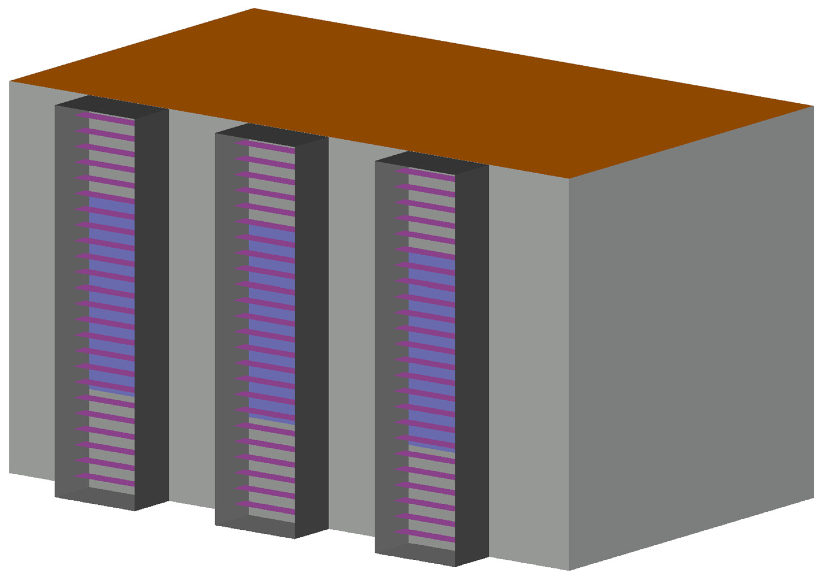
In
Figure 2 is presented the three DSF installed in the virtual chamber. The virtual chamber is used as classroom space occupied with twelve students. The three south-facing DSF are exposed to solar radiation during the day.
The building is located in the south of Portugal, a Mediterranean climate. In the numerical simulation, the air temperature, air relative humidity, wind speed, and wind direction are the external input conditions. These outdoor weather conditions were measured by a weather station installed in the region on a representative winter day. In this situation, the external air temperature varies between 4.5 °C and 13.5 °C, the external air relative humidity varies between 37.2% and 65%, and the wind speed varies between 0.01 m/s and 6.25 m/s.
Each DSF is constituted of four south facing modules. In this situation, the evolution of solar radiation in these modules has its maximum value at midday and its minimum value at sunrise and sunset. The transmitted solar radiation of the glazed surface of each DSF module has its maximum value of around 400 W at noon.
The virtual chamber and the DSF are made of wood and insulated with extruded polystyrene material with a thickness of 40 mm. The virtual chamber is equipped with three windows, with a thickness of 0.4 mm, and the DSF are equipped with two transparent windows, also with a thickness of 0.4 mm: the internal window (of the virtual chamber) and the external window.
The virtual chamber has the dimensions of 4.5 m long, 2.55 m wide, and 2.5 m high and the three DSF have the dimensions of 0.60 m long, 0.2 m wide, and 2.5 m high.
The DSF are equipped with twenty-four adjustable Venetian-type blinds located between the two transparent surfaces. Each Venetian blind has an average thickness of 10 mm, 0.60 m long, and 0.12 m wide.
The ascending DSF airflow (where the energy is produced), which supplies the ventilating system, is channeled through a duct that is connected to the HVAC system located inside the virtual chamber.
2.2.2. Ceiling-Mounted Localized Air Distribution System
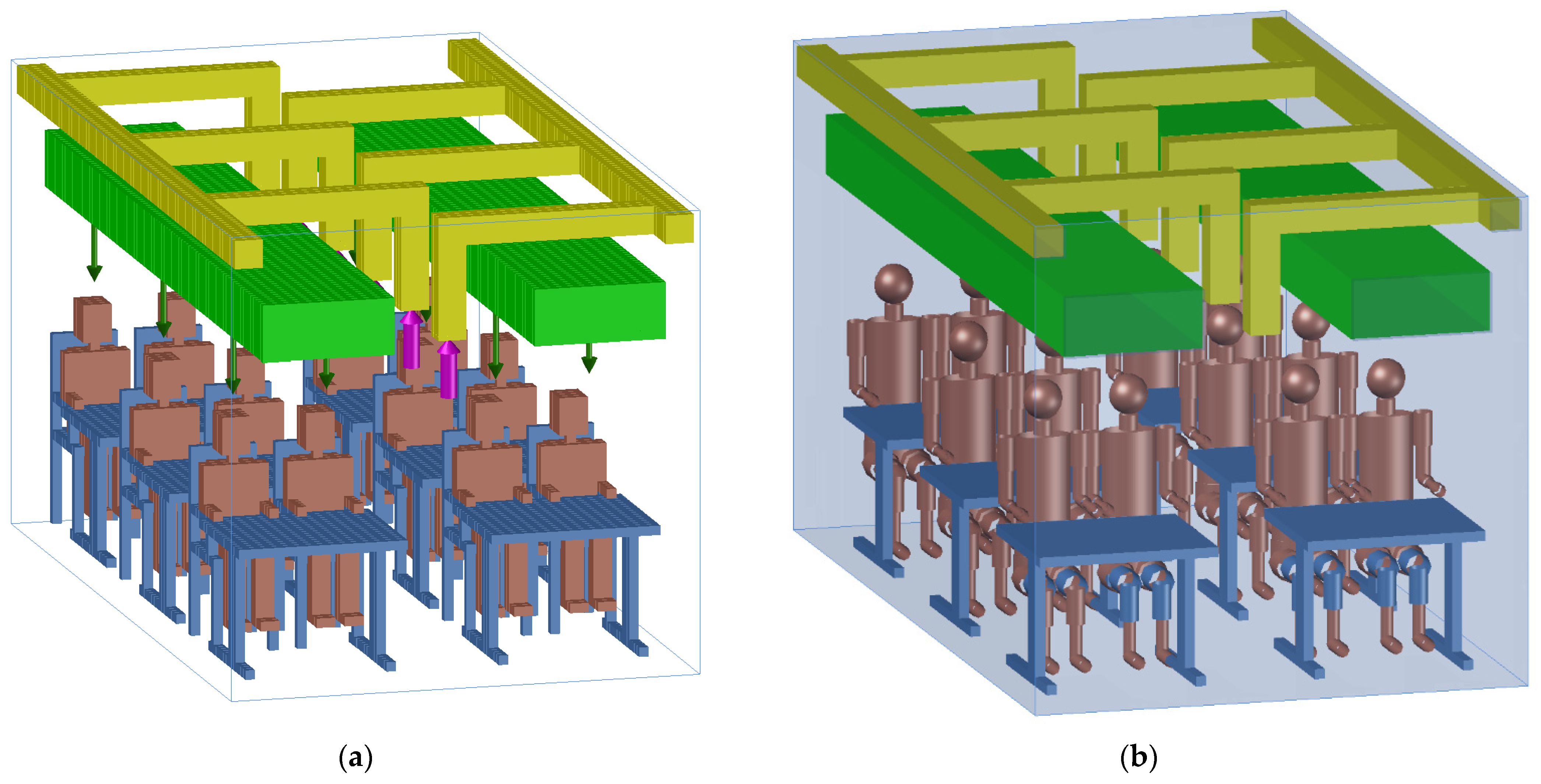
Figure 3 shows the scheme of the virtual chamber, equipped with a ceiling-mounted localized air distribution and exhaust systems.
Figure 3a is associated with the CFD model, while
Figure 3b is associated with the HTR model.
Figure 3b shows the occupants and surrounding surfaces employed in the grid generation and used in the calculation of the heat exchanges by radiation between the occupants and between the occupants and the surrounding surfaces of the desk and ventilation system.
The virtual chamber, which simulates a classroom, is equipped with a ceiling-mounted ventilated system, six desks, twelve chairs, and is occupied by twelve occupants. The ventilation system constitutes an inlet ceiling-mounted localized air distribution system and exhaust ventilation systems, described as follows:
The inlet ceiling-mounted localized air distribution system is built with two horizontal rectangular ducts (represented by the green sections in
Figure 3). Each horizontal rectangular duct considers twelve holes located above the head level and in front to the occupants, that promotes a descendent air jet (see the green arrows in
Figure 3a);
The exhaust ventilation systems are built with six vertical extraction ducts (represented by the yellow sections in
Figure 3). Each extraction duct is constituted of a vertical duct connected to a horizontal duct.
The inlet ceiling-mounted localized air distribution system and exhaust ventilation systems are both located 1.8 m above the floor level.
2.3. Numerical Methodology
In this numerical methodology, the DSF and the HVAC system are presented. The DSF, equipped with internal Venetian-type blinds, is used in the energy production, and the HVAC system is used to promote acceptable indoor thermal comfort and air quality levels.
The numerical simulation was performed for a typical winter day and considered the virtual chamber occupied with twelve students during an occupation cycle defined as follows:
The ventilation cycle, used in the three DSF, considers:
The airflow supply rate, for the cases analyzed, was chosen within a range that allows for the best ADI to be obtained. Depending on the dimensions of the room and in accordance with the standard [
21], this range was chosen considering the recommended airflow rate for an occupancy between eight and twenty-eight people.
This numerical work, which simulates a small classroom, considers four rows of students, namely two located on the corridor side and two located on the window or wall side.
In the numerical simulation, the inlet air velocity of the supply opening is presented in
Table 2 for each case study. The inlet CO
2 concentration is 277.8 ppm and the inlet turbulence intensity is 10%.
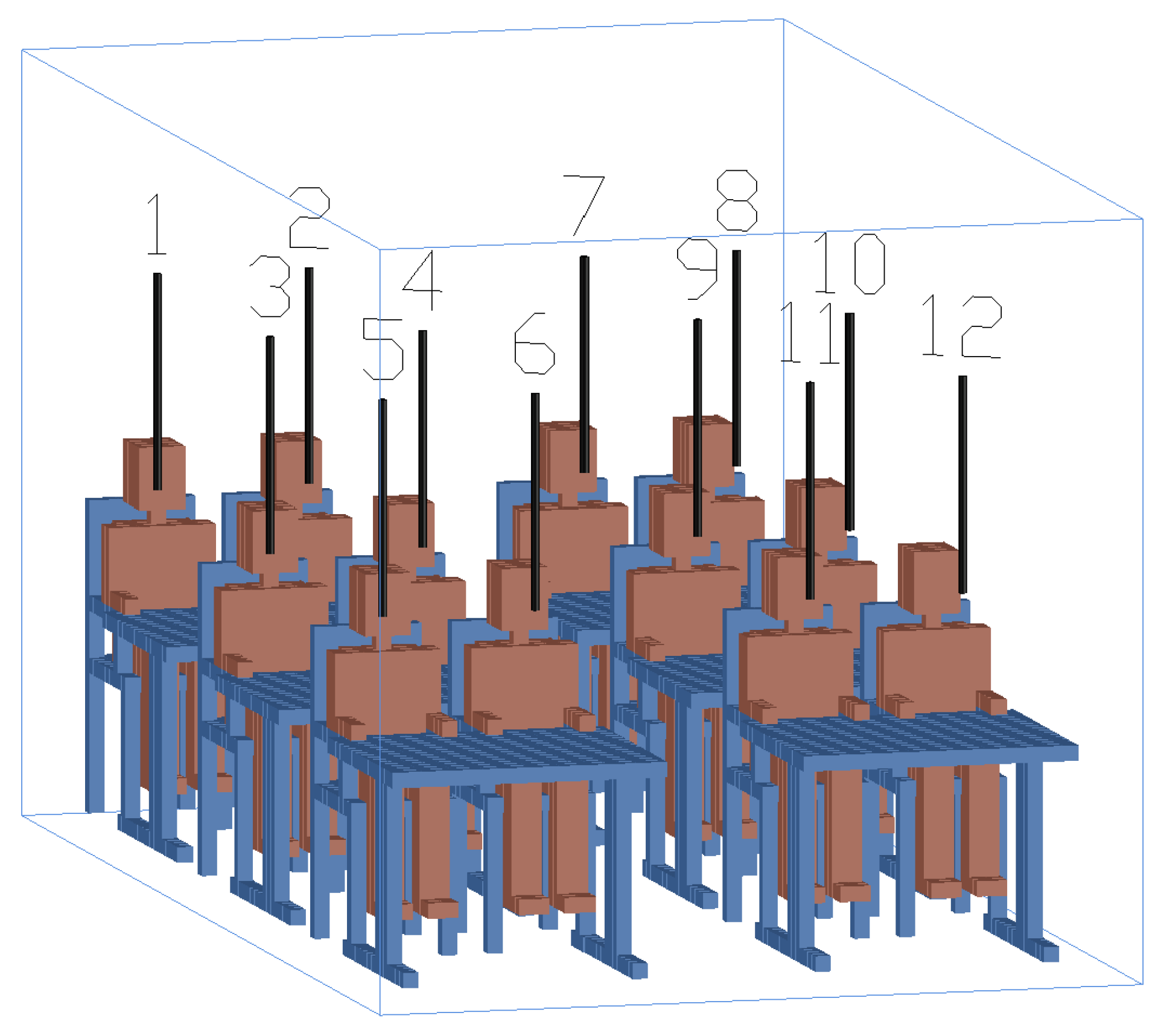
Figure 3a shows the inlet jet airflow (green arrows), located above the head level and in front of the occupants, used in the CFD numerical simulation, while
Figure 4 shows the location and identification (by a number between 1 to 12) of the occupants seated in the virtual classroom, used in the CFD and HTR numerical simulations.
The occupants’ clothing insulation level, used in this HTR numerical model for winter conditions, is 1 clo [
19], and the activity level is 1.2 met [
19]. The insulation clothing level considered in this work, consisted of a long sleeved shirt, dust, pants, shoes, and normal underwear.
The purpose of the methodology implemented is to define the operating point of the designed HVAC system, represented by the airflow rate, which ensures, on average, the best levels of thermal comfort for the occupants and the IAQ in the classroom. The operating point can be selected using the acceptable thermal comfort and IAQ levels criteria or using the maximum ADI criterion. The ADI is evaluated, in relation to the airflow rate, at 10 h, mid-morning, and at 16 h, mid-afternoon.
In addition, knowing the distribution of occupants in the room, we proposed evaluating, depending on the ADI per occupant, the places that have the best conditions of thermal comfort and air quality, if those located next to the corridor, to the walls, front or back (please, see
Figure 4).
It should be noted that this work was developed taking into account the following features:
The geometry of the human body was approximated using a discretization mesh generation by boxes in the CFD model and by cylinders and a sphere in the HTR model;
The winter outdoor environmental conditions for a Mediterranean-type climate;
The most favorable orientation of south facing DSF.
3. Results and Discussion
In this section we provide the numerical simulation results obtained for air temperature inside DSF, thermal energy produced by the DSF system, the ADI at 10 and 16 h, their interpretation, and the main conclusions that can be drawn.
3.1. Air Temperature Inside DSF
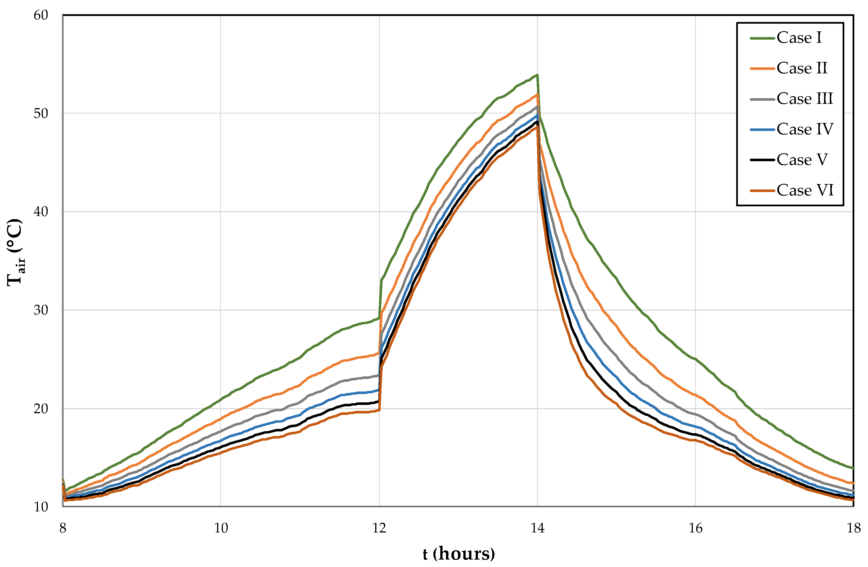
In
Figure 5, the evolution of the air temperature inside the DSF for each of the cases studied is presented. The input data of the inlet and outlet temperatures at 10 h and at 16 h, used in the building thermal response, are presented in
Table 3, while the daily thermal energy produced by the DSF system for each of the cases studied is shown in
Table 4.
The air temperature increases during the morning and the lunch periods, due to the increase in solar radiation, and decreases during the afternoon due to the decrease in solar radiation. For every 0.0389 m3/s increase in the airflow rate (between Cases I and VI) the air temperature inside the DSF decreases, on average, by 2.7 °C between Cases I and II, 1.6 °C between Cases II and III, 1.1 °C between Cases III and IV, 0.8 °C between Cases IV and V, and 0.7 °C between Cases V and VI. This decrease in the air temperature inside the DSF will cause a decrease in the thermal energy (for heating) made available by the DSF to the HVAC system. Therefore, when the airflow rate increases the daily thermal energy production decreases. For every 0.0389 m3/s increase in the airflow rate (between Cases I and VI) the daily thermal energy production decreases 16.2% between Cases I and II, 11.4% between Cases II and III, 8.8% between Cases III and IV, 6.9% between Cases IV and V, and 5.8% between Cases V and VI.
3.2. Air Diffusion Index (ADI) Mean Values
Table 5,
Table 6,
Table 7,
Table 8,
Table 9,
Table 10,
Table 11,
Table 12,
Table 13,
Table 14,
Table 15 and
Table 16 present the evolution of the ADI.
Table 5,
Table 7,
Table 9,
Table 11,
Table 13 and
Table 15 are obtained at 10 h, while
Table 6,
Table 8,
Table 10,
Table 12,
Table 14 and
Table 16 are obtained at 16 h. Case I is associated with
Table 5 and
Table 6, Case II is associated with
Table 7 and
Table 8, Case III is associated with
Table 9 and
Table 10, Case IV is associated with
Table 11 and
Table 12, Case V is associated with
Table 13 and
Table 14 and Case VI is associated with
Table 15 and
Table 16.
The efficiency for heat removal decreases, in general, when the airflow rate increases and the efficiency for heat removal is lower at 10 h than at 16 h.
When the airflow rate increases, the mean value of the PMV index decreases, at 10 h, between 1.63 (Case I) and −0.59 (Case VI), and at 16 h between 1.67 (Case I) and −0.31 (Case VI). The PPD values are lower at 10 h than at 16 h. At 10 h, these values vary between 5.1%, obtained for Case IV, and 57.9%, obtained for Case I. At 10 h, these values vary between 5.1%, obtained for Case V, and 60.1%, obtained for Case I. The results show that acceptable thermal comfort conditions, according to the international standards [
19,
20], are obtained from an airflow rate of 0.1556 m
3/s (Case III) at 10 h and from an airflow rate of 0.1944 m
3/s (Case IV) at 16 h. At 10 h, it is verified in Case III by positive PMV values and in Cases IV, V and VI by negative PMV values; at 16 h, it is verified in Case IV by positive PMV values and in Cases V and VI by negative PMV values
At 10 h, the Thermal Comfort Number varies between 1.7 (Case I), the worst value, and 12.5 (Case IV), the best value; at 16 h, the Thermal Comfort Number varies between 1.7 (Case I), the worst value, and 14.4 (Case V), the best value.
When the airflow rate increases, the CO
2 concentration in the occupant breathing area decreases. The CO
2 concentration in the occupant breathing area at 10 hours is almost the same as at 16 h. In all the cases analyzed, the indoor air quality level is acceptable according to the international standards [
21].
The efficiency for contaminant removal increases when the airflow rate increases. The efficiency for contaminant removal is almost the same at 10 and 16 h.
When the airflow rate increases, the Air Quality Number increases and is similar at 10 and 16 h.
Finally, the ADI varies between 2.6 obtained for Case I and 11.0 obtained for Case V at 10 h, and between 2.6 obtained for Case I and 13.4 obtained for Case V at 16 h. It is higher at 10 h than at 16 h. According to Awbi [
30], in general, an ADI value greater than 10 shows that a ventilation system exhibits good performance. This is achieved for Cases IV and V at 10 h, and for Cases V and VI at 16 h.
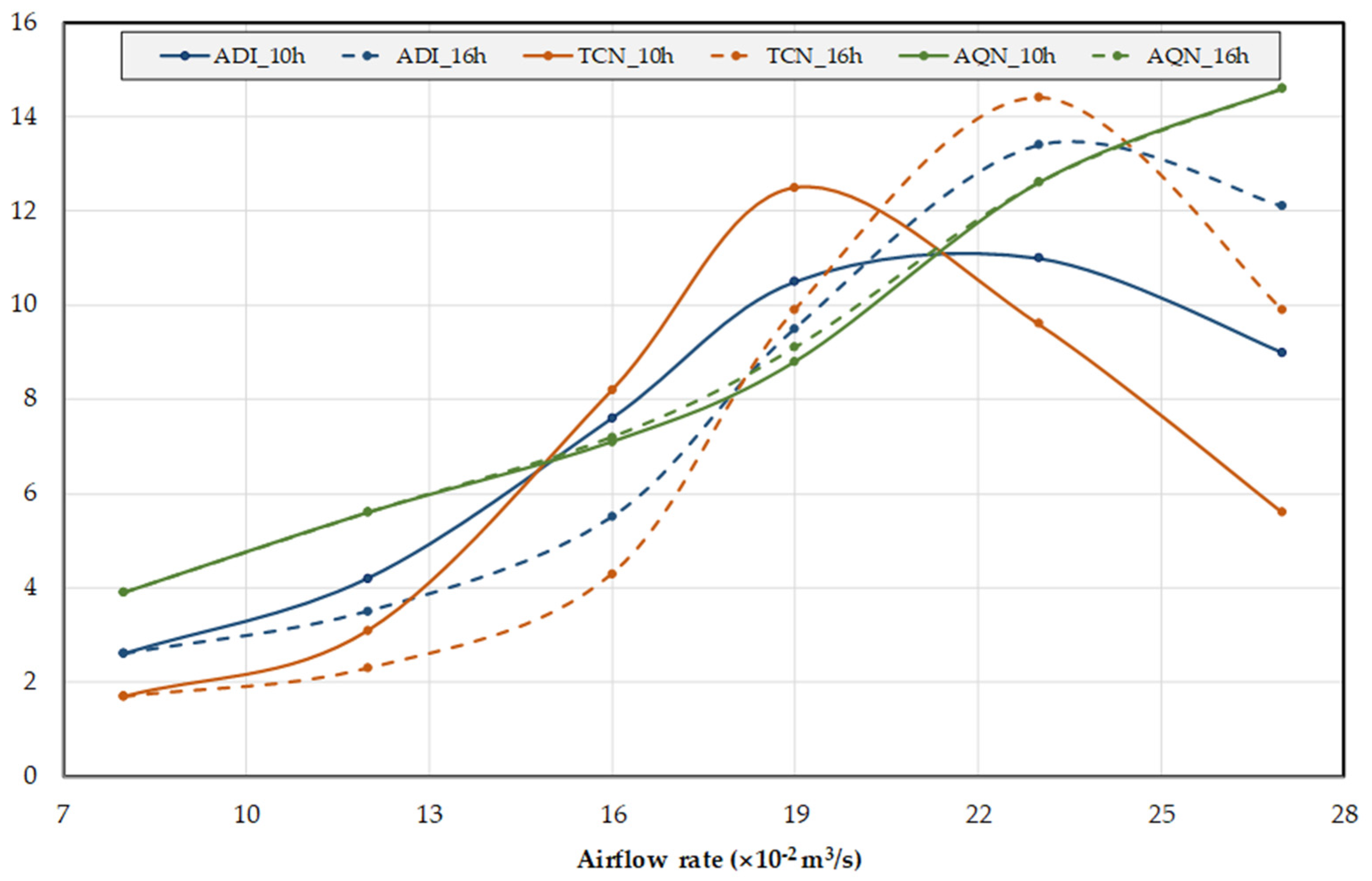
Figure 6 shows the evolution of the Thermal Comfort Number, Air Quality Number and ADI, at 10 h and at 16 h.
When the airflow rate increases, the Air Quality Number increases. Three slopes are verified: the first one up to around 0.185 m
3/s and the third one from around 0.235 m
3/s.
Figure 6 also shows that the Air Quality Number is similar at 10 h and at 16 h.
At 10 h, the Thermal Comfort Number increases up to an airflow rate around 0.195 m3/s and then decreases. At 10 h, the Thermal Comfort Number increases up to an airflow rate around 0.235 m3/s and then decreases. The Thermal Comfort Number is higher at 10 h than at 16 h up to an airflow around 0.230 m3/s, after which the situation is reversed.
Thus, the ADI, which depends on the Air Quality Number and Thermal Comfort Number, increases up to a certain airflow rate and then decreases. The inversion is verified at 10 h for an airflow rate around 0.225 m3/s and at 16 h for an airflow rate around 0.240 m3/s. In general, the ADI inversion is verified for an airflow rate lower at 10 h than at 16 h. This finding is associated with the fact that the Thermal Comfort Number inversion is verified for an airflow rate lower at 10 h than at 16 h.
On the other hand, the ADI is highest at 10 h for an airflow rate below 0.205 m3/s and is highest at 16 h for an airflow rate above 0.205 m3/s. This finding is associated with the fact that the Thermal Comfort Number is highest at 10 h for an airflow rate below 0.205 m3/s and it is highest at 16 h for an airflow rate above 0.205 m3/s.
Regarding the results obtained, the operating point can be selected using the thermal comfort and air quality levels criteria or using the maximum ADI criterion:
Using the indoor air quality level criterion, all situations analyzed are acceptable;
Using the thermal comfort level criterion, the operating point at 10 h is verified between Cases III (0.1556 m3/s) and IV (0.1944 m3/s), while the operating point at 16 h is verified between Cases IV (0.1944 m3/s) and V (0.2333 m3/s);
If the ADI criterion is used, the operating point is obtained at 10 h for an airflow rate around 0.225 m3/s and at 16 h for an airflow rate around 0.240 m3/s.
3.3. Air Diffusion Index (ADI) Detailed Values by Occupant Location
At this point, the thermal comfort and air quality conditions provided by the ventilation system for the occupants will be analyzed, taking into account their locations in the room. The ADI values obtained as a function of the location of the occupants next to the corridor and the walls, as well as the back, center, and front of the room (
Figure 4), will be evaluated. Note that, according to
Figure 4, the occupants seated at the back of the room are subject to the influence of airflow only in front of them. The occupants seated at the center and at the front of the room are subject to the influence of the airflow in front and behind them. However, the occupants located at the front of the room, despite being influenced by the airflow behind and in front, have the presence of a wall in front that deflects the airflow.
In general, the PPD index values obtained for occupants near walls are higher than those obtained for occupants near the corridor, and they are higher for occupants located at the back than at the front of the room. At 10 h from Case III to Case VI, and at 16 h from Case IV to Case VI, all occupants present are at acceptable levels of thermal comfort according to the standards [
19,
20]. The occupants sitting next to the corridor have better conditions than those sitting next to the walls because they are influenced by airflow from the upper air terminal device (ATD) located in front of each person and for what comes from the ATDs located in front of the occupants sitting next to the walls. On the other hand, the occupants sitting at the front of the room have better conditions than those sitting in the back because they are influenced by the airflow from the ATDs located in front and behind them.
As the air extraction system is located in the central area of the room, the concentration of CO
2 in the breathing area of the occupants sitting next to the corridor is greater than that for the occupants sitting next to the walls, although the occupants sitting next to the corridor are under the influence of a higher airflow rate than the other occupants. For an airflow rate less than or equal to 0.1944 m
3/s (Cases I to IV), the occupants seated in the chairs located in the front of the room have lower levels of CO
2 concentration in the breathing area than those seated in the chairs located at the back the room. For higher flow rates, the situation is reversed, that is, the lowest levels of CO
2 concentration in the breathing area occur at those seated in chairs located at the back of the room. However, all occupants have acceptable levels of CO
2 in the breathing area [
21], regardless of the airflow rate used.
For an airflow rate less than or equal to 0.1944 m3/s (Cases I to IV), occupants seated in chairs located near the walls are at higher ADI values than those seated in chairs near the corridor; above this value, the situation is reversed, that is, the highest ADI values are for the occupants seated in the chairs next to the corridor. In general, occupants seated in chairs located at the front of the room have higher ADI values than occupants seated in chairs located at the back of the room. Therefore, the places with the best ADI are located at the front of the room, next to the walls, for an airflow rate equal to or less than 0.1944 m3/s (Cases I to IV), and next to the corridor for higher airflow rates (Cases V and VI).
4. Conclusions
In this paper, the production of renewable solar energy in a DSF system is used for an HVAC system of ceiling-mounted localized air distribution systems, in order to improve the occupants’ thermal comfort and air quality. This numerical study, using an integral building thermal response model and a coupling of an integral human thermal-physiology response and differential computational fluid dynamics models, considers a classroom occupied with twelve virtual students, twelve seats, and six desks. The level of thermal comfort of the occupants was analyzed on the basis of airflow rate, as well as the quality of the air in their breathing zone, according to three criteria: values of the PMV and PPD indexes; CO2 concentration; value of the ADI. Here, six airflow rates were considered. The classroom locations that presented the best ADI values were also identified.
When the airflow rate increases, the results demonstrate that:
The energy production decreases;
The PPD values show that the acceptable thermal comfort conditions for occupants are obtained, at 10 h, for airflow rates between 0.1556 m3/s (Case III) and 0.2722 m3/s (Case VI), and at 16 h for airflow rates between 0.1944 m3/s (Case IV) and 0.2722 m3/s (Case VI);
The CO2 concentration decreases. However, in all situations, the air quality level conditions are acceptable;
The ADI increases initially but after a certain airflow rate it decreases. The inversion is verified at 10 h for an airflow rate around 0.225 m3/s and at 16 h for an airflow rate around 0.240 m3/s. The ADI is higher at 10 h than at 16 h until an airflow rate of 0.205 m3/s is provided. After this airflow rate, the ADI is lower at 10 h than at 16 h.
The operating point can be selected using the acceptable thermal comfort and air quality levels or using the maximum ADI criterion. Using the indoor air quality level conditions, all situations analyzed provide acceptable conditions. Using the thermal comfort level criterion, the operating point at 10 h is achieved between airflow rates of 0.1556 m3/s and 0.1944 m3/s, while the operating point at 16 h is achieved between airflow rates of 0.1944 m3/s and 0.2333 m3/s. However, if the ADI criterion is used, the operating point is obtained at 10 h for an airflow rate around 0.225 m3/s and at 16 h for an airflow rate around 0.240 m3/s.
By carefully choosing the optimum airflow rate, it is possible to manage the production of thermal energy in the DSF more effectively. Note that for a lower production of thermal energy, which is associated with higher airflow rates, it is possible to obtain acceptable levels of thermal comfort for the occupants according to the standards, and simultaneously obtain high values of the ADI, which denotes a good performance of the HVAC system. A more detailed study of the ADI values obtained by occupants allowed us to identify that the places located in the front of the room and close to the walls, in general, were those with the best conditions of thermal comfort and air quality in the breathing area. The implemented methodology also shows that it is possible to adapt the best airflow rate for the time of day in order to ensure the best performance of the HVAC system with regard to the maintenance of acceptable conditions of thermal comfort and air quality for the occupants.
Finally, we highlight the novelty introduced by the research software used, which made it possible to analyze, in an integrated way, the energy produced by the DSF, the level of thermal comfort, the level of air quality, and the ADI, either as a function of average values or depending on the values obtained from occupant to occupant.


