1. Introduction
At the Paris Climate Agreement in December 2015, almost 190 parties signed the agreement to limit global warming to 1.5 °C [
1]. The main causes of global warming are manmade greenhouse gas emissions. According to the United Nations Environment Programme (UNEP), the overall amount of carbon emissions related to the building sector adds up to 38% [
2]. This share not only comprises the building operation (28%) but also includes the emissions from the building industry caused during the production of the building materials, especially concrete and steel. This outlines the potential and, furthermore, demands the urgent need for action to decrease emissions.
Within the existing norms and codes for buildings, the constant, annual static emission factor plays a key role as a parameter for the evaluation of the emission balance. However, it is due not only to climate change and the rise of electrical, regenerative energy sources such as photovoltaic (PV) or wind energy, but also, according to the Fraunhofer Institute for Solar Energy Systems, to the electrification of building technology, which changes the circumstances on the supply and demand side [
3]. This leads to daily and seasonal variability in the price and emissions of the German power grid.
Under these circumstances, especially with the system of emission balance boundaries of the building operation, the common concept of a static emission factor should be criticized. This, consequently, leads to the necessity of the examination of the dynamic emission factor.
1.1. Objective
With its climate protection plan, the German government aims to be climate neutral by 2045 [
4]. One component of this plan is a climate-neutral building sector. National and international legislations, such as the German Building Energy Code (GeG), have set out requirements for the buildings and the technologies contained in them in order to promote an increase in the energy efficiency of the building sector and a transition to renewable energies [
5]. The research field of building technology addresses these challenges with thermal simulation models to analyze the effects on the energy efficiency of buildings (e.g., load management). Within the evaluation of these processes, the emission factor plays a key role, with climate neutrality becoming the overarching goal of modern building projects. In addition to the development of a concept and simulation process, the effects of a dynamic emission factor were analyzed, under the general hypothesis of this paper:
Using dynamic, hourly emission factors to calculate the CO2 emissions for the building operation generates emission savings, which are not represented in the common calculation concept based on static, imprecise data.
To evaluate this hypothesis and to facilitate a deeper understanding of the concept of the dynamic emission factor and its impact, this paper explores the following research questions:
How does the consideration of a dynamic instead of a static emission factor impact the CO2 balance of a building operation?
What potential does an emission-optimized load control have?
How does an increased storage capacity influence performance?
How big is the impact of the dynamic emission factor calculation on the overall transformation of the German electricity grid?
1.2. Methodology
This paper proposes the concept of using the dynamic emission factor in thermal building simulations to more accurately depict the emission balance of a building. After an initial literature review establishing the current state of the research and defining the research gap, this paper presents the weather and electrical power-grid data and outlines the simulation setup (as displayed in
Figure 1), which also defines the concept for the analysis of a dynamic emission factor.
For this purpose, the dynamic thermal simulation (Plug-In TRNLizard for Rhino 7) and the radiance simulation (Plug-In HoneyBee for Rhino 7) form the basis of feeding a system model simulation (Grasshopper/Python) to evaluate the emission balance in a second step. After introducing the concept and the simulation model, the potentials of this strategy are presented and further outlined in the final outlook through potential future research projects with the aim to achieve the previously mentioned climate neutrality.
1.3. Literature Review
Within this research field, a couple of studies have already taken into account the hourly emission-factor profile of the German power grid. They comprise first studies that were conducted to detect the energy- and emission-saving potential [
6,
7,
8,
9]. These studies all focus on the concept of the average-emission factor. A second approach to dealing with a dynamic emission factor is using the marginal emissions method, but this approach is not considered in this paper nor in this literature review. The following gives a quick overview of the aforementioned studies and defines the research gap of this paper.
Regett and Heller, in 2015, showed that there is a notable variation between static and dynamic emission factors in the power grid. The effect is very easily detectable in the mid-day hours in the summer months with the increase in the photovoltaic energy, as well as a general increase in the winter months with aggrandized wind speeds and, thus, an increase in the wind energy. According to the authors, a CO
2-optimized approach with dynamic emission factors is very suitable [
6].
In their work “Dynamic Prospective Average and Marginal GHG Emission Factors—Scenario-Based method for the German Power System until 2050”, Seckinger and Radgen developed a method to generate an hourly emission factor based on the German power grid. They also outlined the day and night variances in the summertime, as well as the seasonal variability and the advantage in the winter months. Furthermore, they outlined the advantages of these high-resolution analyses [
7].
Wörner et al. also demonstrated a method for the dynamic electrical emission factor. In their work, they analyzed the effects of a CO
2-emission-optimized control compared to a customary control strategy of the building technology of a residential building with a heat pump. According to their study, this CO
2-optimized operation opened up huge energy- and emission-saving potentials, with these potentials further increasing with bigger buffer storage in the building technology system [
8].
In 2019, Müller and Wörner presented a second paper: “Impact of dynamic CO
2 emission factors for the public electricity supply on the life-cycle assessment of energy efficient residential buildings”, in which they used the CO
2-optimized control in a thermal building simulation to calculate the emission balance for a residential house with a heat-pump system. They could also detect a deviation within the single-digit percentage range, as the dynamic version performed worse considering the emission balance. This is based on the fact that power consumption mainly takes place in the winter months when there is no PV yield. They further analyzed the system for the years 2030 and 2050, under the assumption of an expansion of renewable energies, which reduces the CO
2 emissions and increases the difference between the static and dynamic approaches [
9].
Overall, all authors agree on the need for a dynamic, hourly emission factor. Only through this can the real effects and potentials of single-efficiency measures be quantified, and only with this information can the regulation of the load management of the electric power grid be represented correctly [
7]. These studies only focused on a residential building with a heating system. The authors highlight the necessity of considering further areas of consumption to better evaluate the effects and to differentiate building usages and locations, such as hot-water power consumption, or a cooling system in the summertime [
9].
2. Fundamental Data
To represent the correct, local metrological and energetic circumstances and to connect the data in the right manner, this paper uses the hourly data for the weather and the power grid of the year 2018. In the following, this chapter first describes the weather data, and the data of the electrical power grid, displayed in detail, to generate a general insight for the following analyses.
2.1. Weather Data
The weather data have an influence on the performance of a building and its energy balance. As of the year 2018, according to the DWD (Deutscher Wetter Dienst; In Englsch: German Weather Forecast Services), 10.5 °C represents the highest average temperature of the year since data recording started for the location of Munich [
10]. For the simulation, the weather station closest to the location of the building was chosen. In general, a validation of the weather data was carried out to prevent uncertainties [
11]. The DWD already provides a validated data set that includes air temperature, dew point temperature, relative humidity, air pressure, atmospheric radiation, horizontal radiation, direct normal radiation, wind velocity, and wind direction.
2.2. Power Grid Data
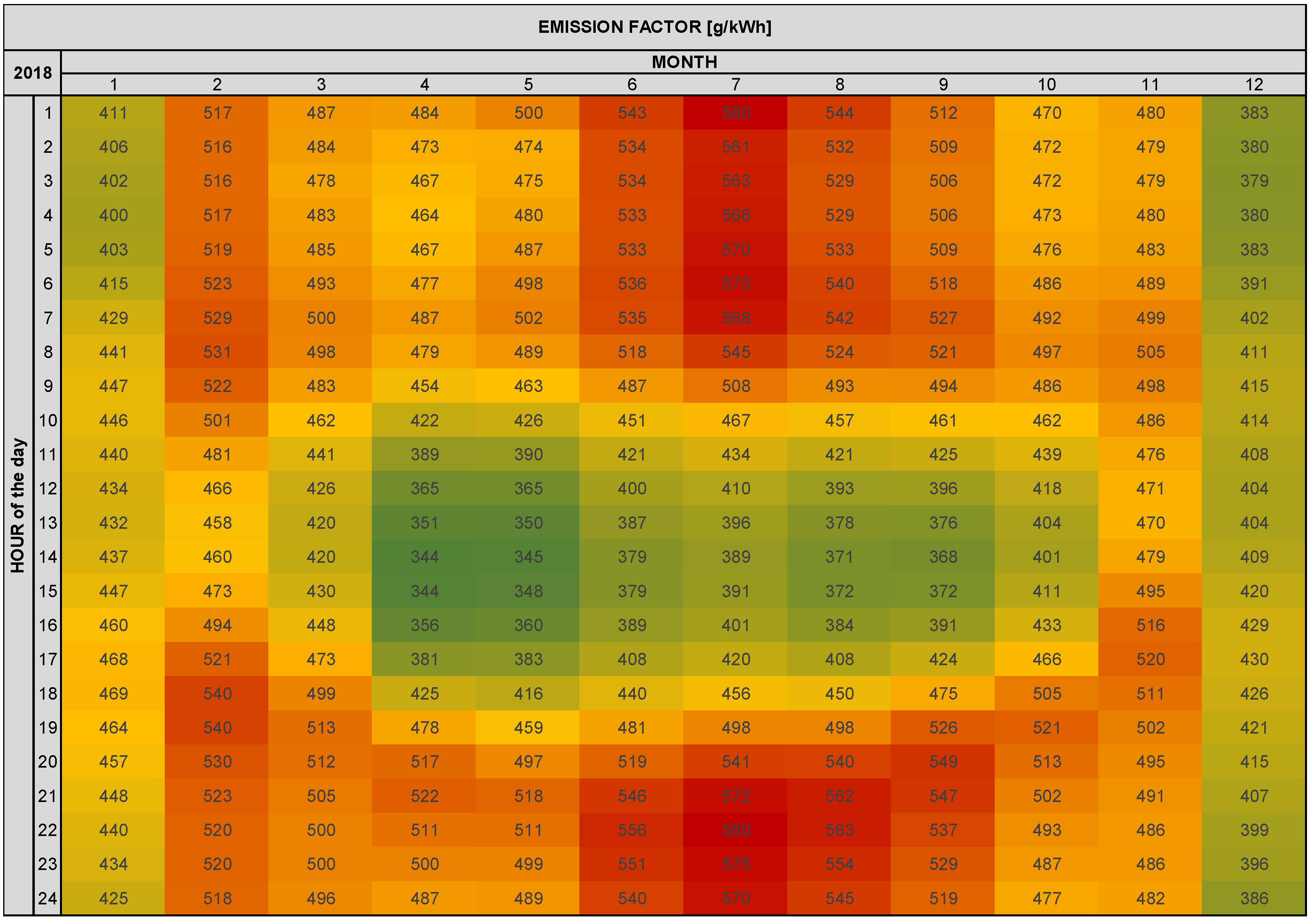
The data set for the dynamic emission factor is provided by the think tank Agora Energiewende. The data set comprises the production capacity, level of consumption, electricity import and export, and the electricity price of the German power grid for the years 2011 to 2020. From these values, the Agora Energiewende calculates an hourly value for an emission factor, as presented in
Figure 2 [
12].
The figure illustrates the fundamental daily and seasonal characteristics of the emission factor. In general, the values in the noon times, especially in the summer, are lower than those at night times. Further, in the winter months, particularly December and January, the values are lower over the course of the day. Both characteristics are related to the higher share of regenerative energies in the summer with the photovoltaic and in winter with the wind energy.
The second approach used in this paper considers the energy price. For consumers, one of the main motivations to save energy is the costs, and as the energy price is at least partly linked to the emission factor, an economic approach is also targeted. An in-depth look into the data depicts that the electrical energy price on the market varies frequently over the course of a day, while performance remains steady over the course of a year. The energy price not only depends on the related emissions but also considers aspects such as the import, export, and availability of certain energy resources. In general, the overall price contains a variety of fixed shares, which leads to a very low fluctuation.
The different characteristics of the emission factor and the electricity price approaches will be analyzed to save energy and/or CO
2. In addition, a future scenario for 2040, also provided by Agora Energiewende, will evaluate the potential development of these strategies. The individual assumptions are the phase-out of conventional energies, the extension of regenerative energies, the increase in the electrical energy demand (E-Mobility, heat pumps, hydrogen production, etc.), and the flexibility in the industrial energy demand. These assumptions are based on the study of 2021: Klimaneutrales Deutschland 2045 (Climate neutral Germany 2045) [
12].
According to these boundary conditions, the share of regenerative energies increases significantly, which in most cases leads to a significantly lowered emission factor. The daily variation in the emission factor is conspicuous and occurs mostly in summer times.
3. Thermal and Radiance Simulation
This chapter outlines the fundamental models and assumptions of the dynamic thermal and radiance simulation. To evaluate the influence of the dynamic emission factor, a thermal and radiance simulation was performed. This chapter describes the principles and the baseline model for this analysis. To calculate the energy demands on an hourly basis, a thermal building simulation was performed. The software used to perform such stationary processes is TRNSYS (Version 18) [
13]. With its Plug-In TRNLizard for Rhino 7, this software environment provides a modular base for thermal analyses and forms the connection to the Plug-In Ladybug Tools. Within this additional tool kit, further investigations can be performed. The Plug-In HoneyBee focuses on the radiant performance of a building. Based on the hourly solar radiation on a building’s PV collectors, the overall solar yield can be determined [
14].
3.1. Thermal Simulation
The inputs for the thermal simulation are the information about the building, the construction details, and the usage, which are used to calculate the energy demand.
To keep the focus of this paper on the dynamic emission factor, the thermal simulation is only described briefly. The north–south-oriented office building for the base case model is located in the city of Munich and is partly supplied with natural and mechanical ventilation. The heat energy is provided by a geothermal heat pump with buffer storage and floor heating to transfer the heat to the rooms. The COPs for the heating, domestic hot water, and ventilation are assumed to be 5.24, 3.30, and 4.20. The office areas with mechanical ventilation are supplied with cooling ceilings using groundwater. The natural ventilation also includes nighttime flushing. Venetian blinds, with an fc-value of 0.2, are included to prevent overheating in the summer period. The shading system is controlled according to the solar radiation.
The usage and device profiles of the rooms are simulated according to the “Raumpilot Grundlagen” [
15]. The U-values are connected to the German reference values according to the GeG (Gebäudeenergiegesetz; German building energy code) (external wall 0.167 W/(m
2K), internal wall 0.556 W/(m
2K); roof 0.177 W/(m
2K); window 0.923 W/(m
2K), floor slab 0.182 W/(m
2K)), and the thermal bridges are considered with 0.05 W/(m
2K) [
5]. The heat capacity varies between 50 and 130 Wh/(m
2K), which represents a medium-duty design according to DIN 4108-2 [
16].
Further, the usage of the building determines the internal loads. This includes the internal gains considering people, devices, domestic hot water, and the power for lighting. These assumptions are connected to the reference values of the DIN V 18599 [
17].
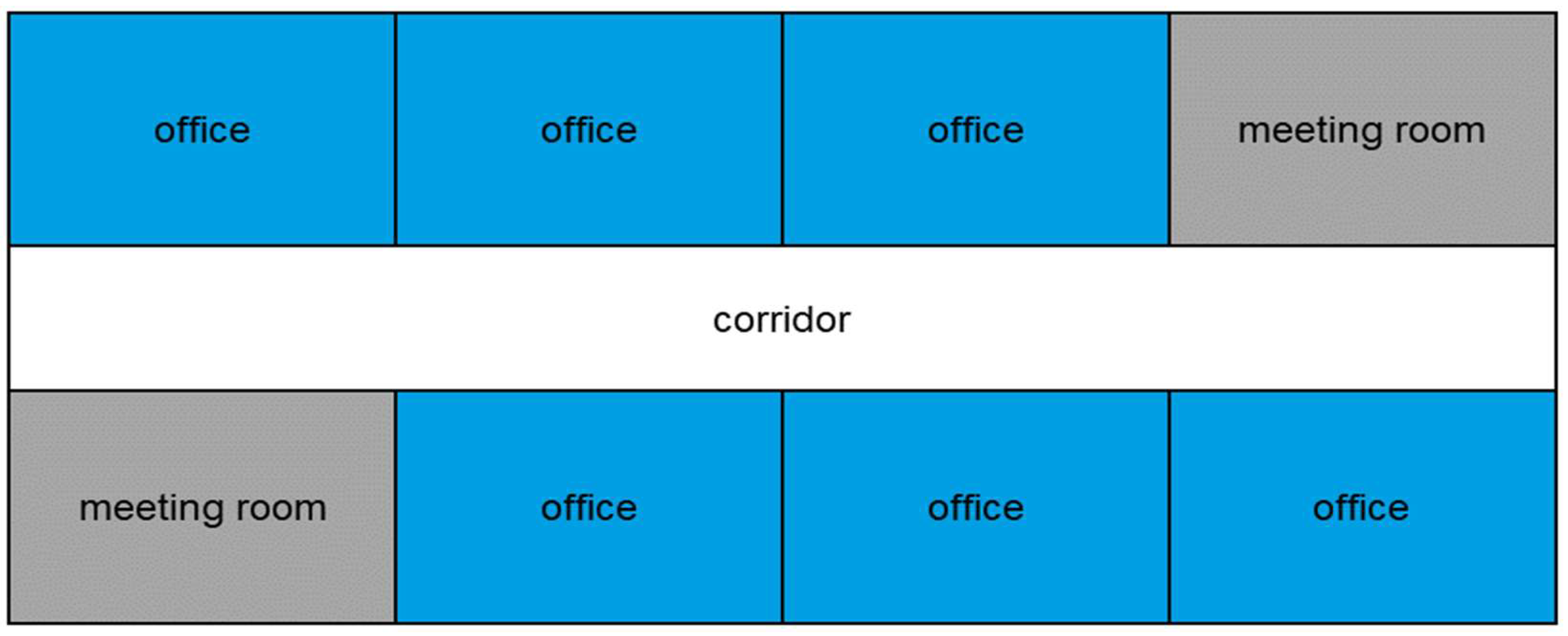
Based on these factors, information zones are formed. These zones interact with the adjacent zones as well as with the outdoors to calculate the annual energy demand. In total, the office building is 1690 m
2. The standard arrangement of the rooms according to Jochen and Loch (illustrated in the following
Figure 3) is used in all five stories of the building.
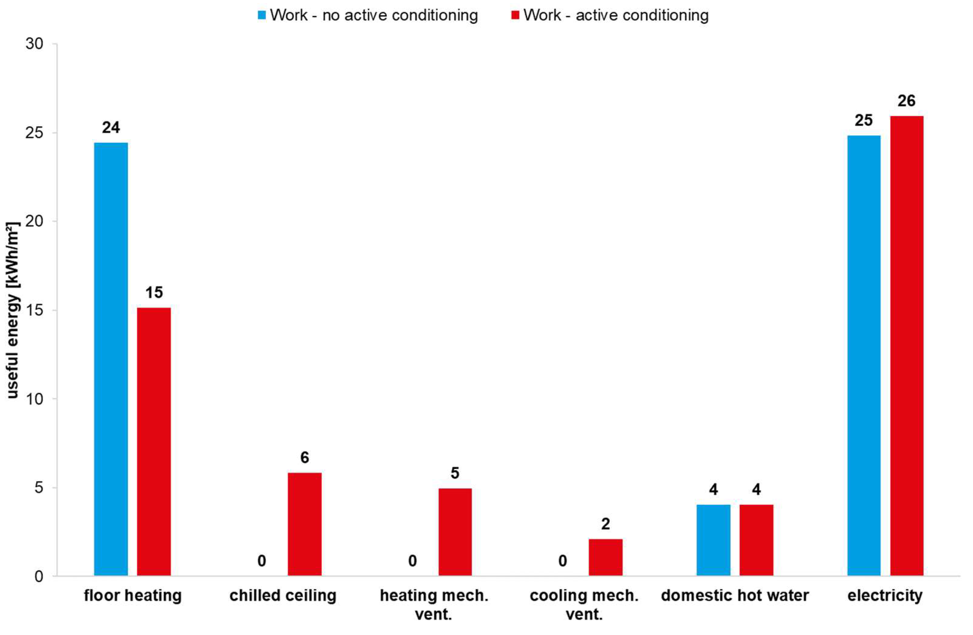
The results of the thermal simulation are evaluated according to the energy demand, thermal comfort represented by the specific energy demand in kWh/m
2a, and the operative temperatures of a south-oriented office room.
Figure 4 illustrates the high energy demand mainly responsible for the north-oriented office rooms. A cooling demand for the variant with active conditioning occurs during the middle of the day during the summer. The nighttime ventilation and the Venetian blinds can cover this cooling demand in the variant with natural ventilation, which, on the downside, causes an increase in the heating demand in the colder seasons.
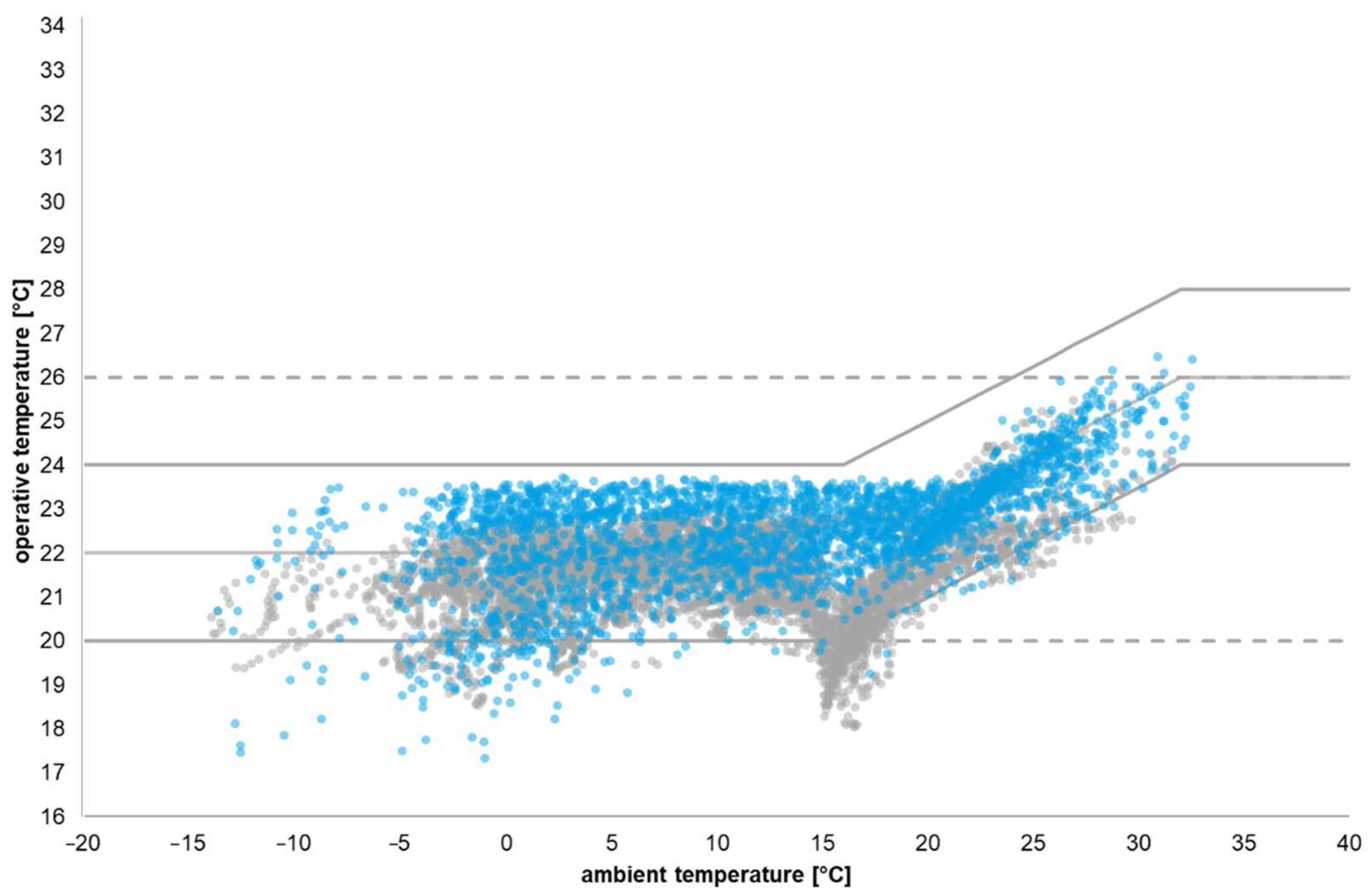
Subsequently, in
Figure 5, the operative temperatures of areas with natural ventilation are illustrated. The comfort boundaries of 20 and 26 °C were set based on the DIN EN 16798-1 for the analysis. It should be recognized that there is no cooling energy needed, but especially in the winter times, the ventilation causes below-comfort-temperature hours (own translation, from German: Untertemperaturgradstunden). There are no over-comfort-temperature hours (own translation, from German: Übertemperaturgradstunden) but 79 h below a comfortable temperature, which is still acceptable according to the norm [
18].
3.2. Radiance Simulation
Besides the local weather data, the software Plug-In HoneyBee for Rhino 7 needs a couple of further inputs to calculate the solar yield. To increase the solar collection, the solar panels on the flat roof are oriented east and west, with a tilt of 12.5° to avoid the self-shading of the modules. This orientation collects more sunlight in the morning and evening hours and increases the share of the usage of electricity. The distance to the fascia is set to 0.5 m, where the distance between the models amounts to 0.3 m. This adds up to a total area of 214 m2 of solar panels.
To calculate the solar yield, a detailed model according to Heydenreich et al. (2008) was used. His concept considers the fluctuation of the solar panel temperature and the solar radiation to calculate an hourly coefficient of performance [
19]. The efficiency of the panel and increase in the power of the system can be calculated as represented in the following equations. The individual parameters of the equations are selected according to the implemented system components:
Via Microsoft Excel and the programming language Python, these equations are implemented into the software to calculate the solar yield. The solar yield of the whole system amounts to 29 kWh/m2 which adds up to 49 MWh per year. With a closer look at the data, the seasonality of the photovoltaic system can be observed.
4. System Model Simulation
Inputs flowing into the building system model are the results of the thermal and radiance simulation, as well as the emission data. The main output is the emission balance considering various storage models. The balance boundary for these analyses is the operation of the building. Explicitly excluded in this paper are all the phases of the process connected to the production, transportation, and disposal of the components. The main goal is to evaluate the dynamic emission factor, taking various system set-ups and load-control strategies into account. The following sections of this chapter outline the fundamentals concerning the storage models, the system configurations, the evaluation indicators, and the load-control strategies.
4.1. Storage Models
The building system model displays thermal (heating and hot water) and electrical battery storage. This means there has to be enough charging capacity within the storage. or else, in the case of empty storage, additional energy charging occurs (e.g., using a heat pump). The fundamental parameters and variables for the model are storage capacity, rated charging capacity, unloading capacity, control strategy for charging, limit temperature for charging, storage losses, and storage efficiency. The discharging capacity is equivalent to the simulated energy demand of the building simulation without losses of transportation (e.g., cables or ducts). The general outputs of the storage model are the reservoir storage level, the loading capacity, and the auxiliary power.
The system configurations, including photovoltaic systems with battery storage, supplement the inputs with the PV productions. The additional outputs are the PV effective output and the rest of the PV effective output. In general, the electrical power of the PV system is used to load the storage. The thermal storage in that case uses the heat pump to charge up. The next section outlines the system configurations in detail.
4.2. System Configurations
This paper analyses four system configurations. The system configurations represent state-of-the-art system configurations to transfer, store, and reuse photovoltaic energy and can be implemented in various building configurations or usages:
SC1: Thermal storage
SC2: Thermal storage + battery storage
SC3: Thermal storage + PV
SC4: Thermal storage + battery storage + PV
The thermal storage is divided into two storage areas for heating and hot water. The battery storage provides energy for the user electricity requirements and the power for the circulation pump and the heat pump.
The capacity of the thermal storage is designed for a 1-day period. According to the day with the highest energy demand, this leads to a capacity of 550 kWh for heating and 25 kWh for hot water storage. The capacity for the battery is 90 kWh, following Weniger et al. who showed that, above 2 kWh capacity per kWp, the level of self-sufficiency does not rise anymore [
20].
SC1: In the basic system configuration, two thermal storage areas are loaded according to the simulated energy demands. The grid fully covers the electrical energy.
SC2: The second variant operates identically except for the battery storage areas. This capacity is used to buffer the electrical energy demand.
SC3: In the third scenario, power from the installed PV system is integrated into the system. Whenever possible, the PV power is used for direct usage (user electricity and electricity for the pumps and the heat pump). Beyond that, the storage for heating is utilized and the storage for hot water is filled. Only after those steps is the surplus power fed into the grid.
SC4: The last system configuration is similar to SC3 besides the integration of battery storage. The usage is prioritized as follows:
Direct electrical usage
Feeding into heating storage
Feeding into hot water storage
Feeding into battery storage
Feeding into the electrical grid
4.3. Indicators
To evaluate the balance of the various system configurations, the emission in kg CO2, the cost for electricity in EUR, and the network load in kWh are used as indicators. This section outlines the general calculation processes of the individual indicators. Exceeding the focus of this paper, the detailed calculation processes are not displayed.
The emissions are summed up over the year according to the energy demand and the corresponding emission factor. With a PV system, a specific CO
2 credit is calculated for the surplus power, which is fed into the grid. To evaluate the effect of the dynamic calculation, the static and dynamic calculation process is presented in the following equations.
The costs for electricity are identified according to the domestic electricity price. Within this value, the trading price only holds a small share, which leads to no notable difference between a static or dynamic calculation. A credit for the integrated electricity is calculated but not displayed in the following equation:
Besides the emission factor and the domestic energy price, the data of Agora Energiewende also provides the consumption and the production within the grid. Their ratio represents the self-defined indicator net load. The data display a surplus of energy in the early morning and late evening hours in the summer period. In the winter months, no correlation between the emission factor and the net load can be seen. The following equation represents the calculation process for the net load:
4.4. Load Control Strategies
The load control strategy defines the points in time when to fill up the storage. This paper analyses four different control strategies that can be divided into two categories and thereby address either the energy price or the emission factor. The first category comprises a simple, constant period control strategy, whereas the second category uses a predictive method to determine the minimum of a parameter. In this paper, the parameter is represented by the energy price or the emission factor:
Energy price simple (EPs)
Energy price predictive (EPp)
Emission factor simple (EFs)
Emission factor predictive (EFp)
The simple control strategies found in the previously outlined data analyses. Thereby daily constant load periods are defined to make use of the low periods of the energy price and the emission factor. For the energy price, this results in a 6 h loading period between 00:00 and 06:00 a.m. when the trading energy prices are low. Considering the emission factor for the simple control strategy, the loading periods shift to 10:00 a.m. to 04:00 p.m. to use the PV energy production during the daytime.
The predictive control strategy in that sense does not represent a real, data-driven prediction. It uses the annual net data and searches for a minimum within the next 24 h at each time step. Based on this process, a 5 h loading period is then implemented to fill up the storage. This concept uses the data to define the minima for the energy price as well as for the emission factor.
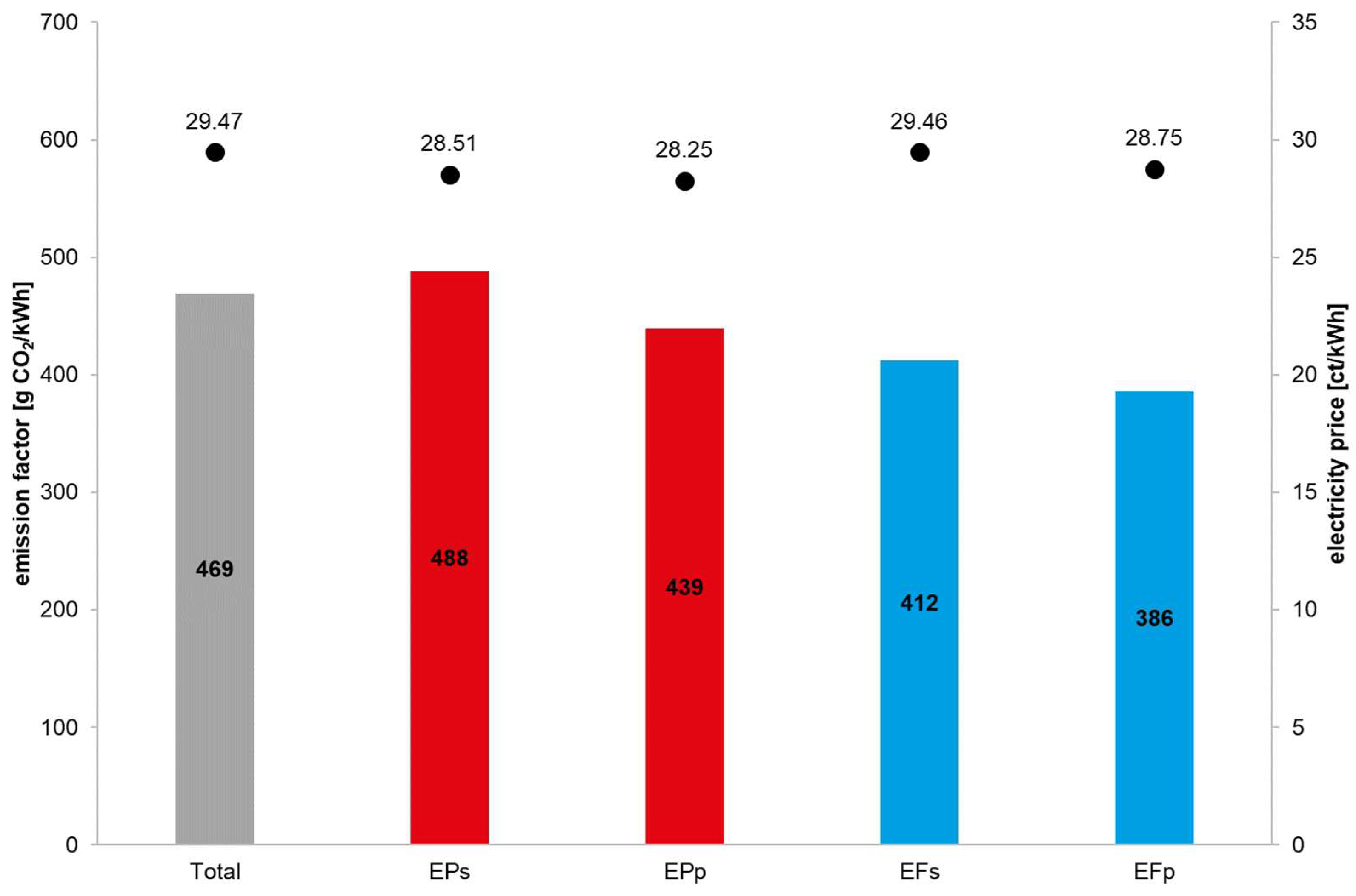
Figure 6 illustrates the overall annual CO
2 emissions of the four control strategies in comparison to the average baseline, indicating the potential of the emission-based control strategies. The black dots represent the overall, annual energy price, where the energy-price-optimized controls consequently show the lowest values.
5. Results and Evaluation
This chapter presents the results and their evaluation. The following sections outline the individual research questions and evaluate the results.
5.1. Difference in CO2 Balance between Dynamic and Static Calculation
The following results are based on the load control strategy EPs, taking the energy price into account. The disparities between the four load strategies are addressed by the next research question.
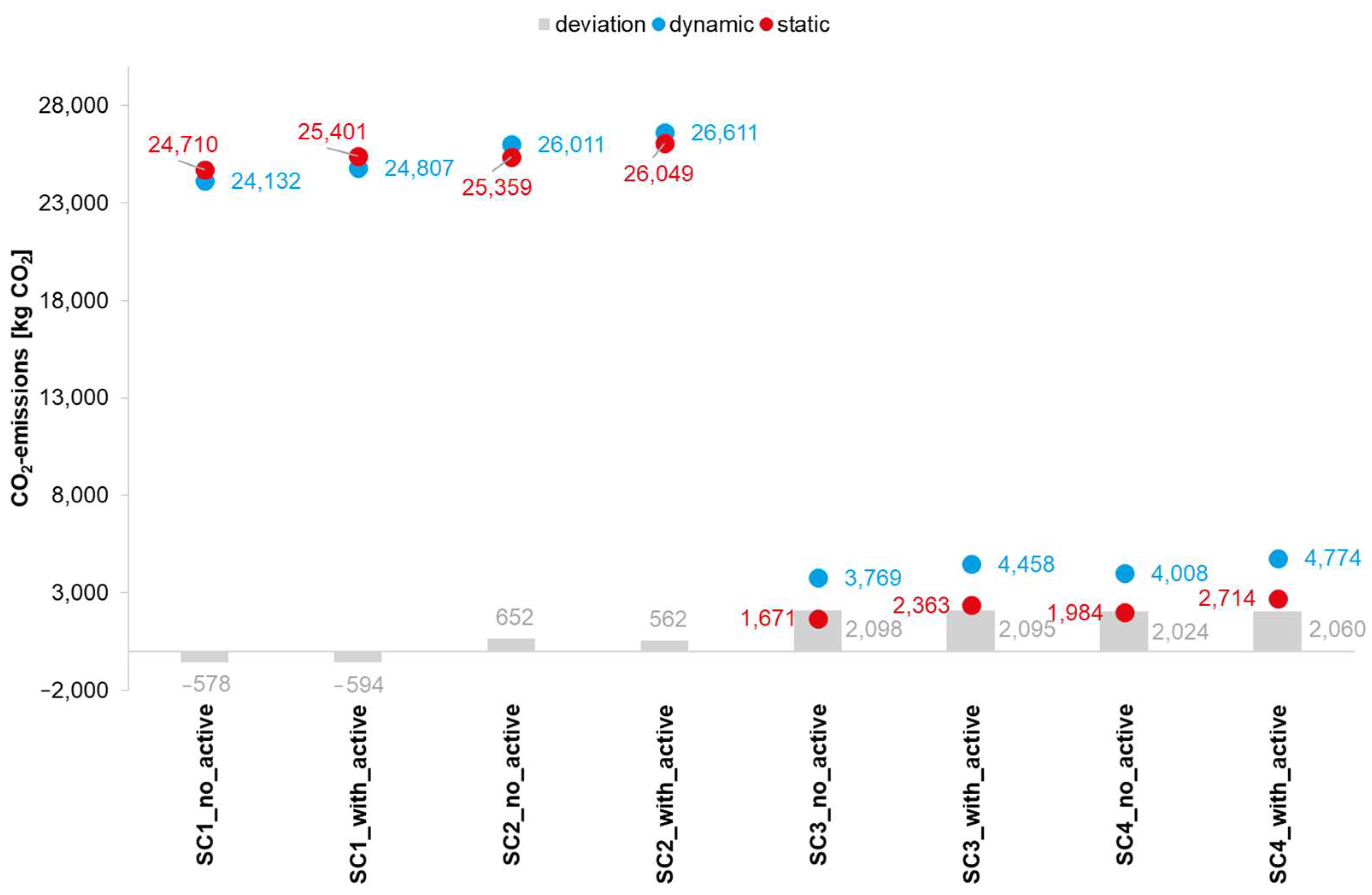
Figure 7 shows a variety of data addressing the CO
2 emissions on the y-axis and the different system configurations for an office building with natural and mechanical ventilation, calculated with a dynamic and static emission factor. It further shows the differences between the two calculation approaches.
If the energy source is a heat pump, the emissions are mainly influenced by the user power demand. If there is no battery (SC1), a significant difference between the static and dynamic approach can be observed. For both variants—with and without mechanical heating—the emissions for the dynamic approach are lower because the main electrical demand occurs around noon.
Furthermore, it can be seen that the emissions increase when implementing a battery storage. This is mainly caused by the energy-price-oriented control strategies, besides the general storage losses. Integrating a PV system reduces overall emissions significantly. This is due to the efficient usage of PV electricity (SC3 and SC4), as well as the electricity for the heat pump. However, again, the overall static emissions are lower based on the credit note in the calculation process.
In a heat-pump-based building configuration, the user’s electricity dominates the overall consumption. With no storage or too-small storage, the emissions are mainly dependent on the user’s electricity demand. The answer to the question presented initially can be divided into two. With a non-emission-optimized control strategy and without a PV system, the difference between a dynamic and static approach is negligible. With a PV system, significant differences can be identified. This again leads back to the credit effect of the calculation method. Going beyond the focus of the analyses, the following sections will only present the simulation results with mechanical ventilation, as both variants produce similar results, as confirmed in the first research question.
5.2. Potential of an Emission-Optimized Load Control
This section answers the previous research question. All storage load strategies, as well as all three indicators, were used for the analyses. Based on the huge number of variants and data, not all the results are visualized in this paper.
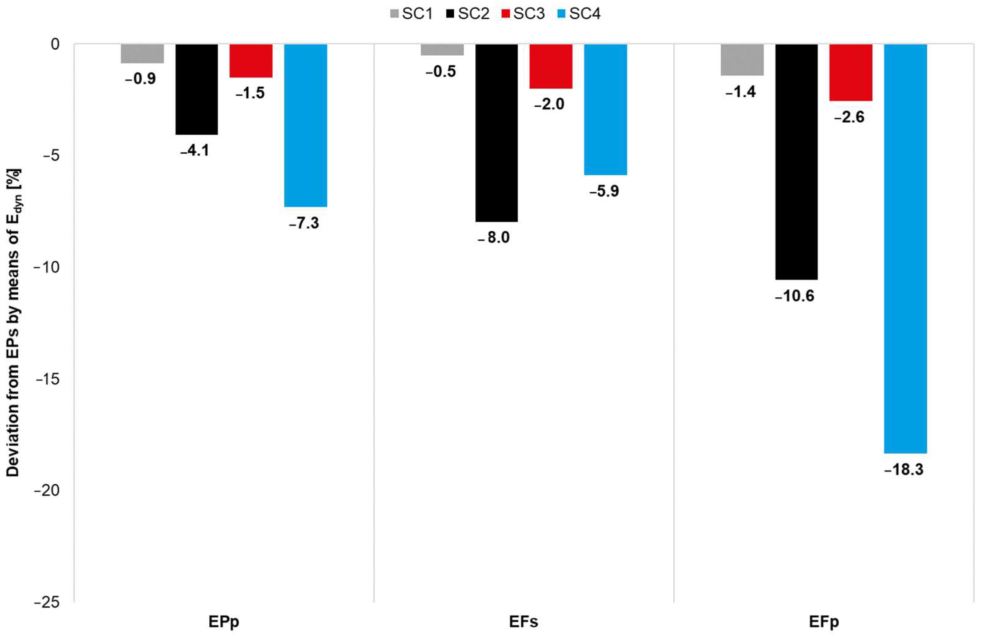
To evaluate the emissions,
Figure 8 displays the percentage deviation between the individual variants and the previously outlined results, considering the simple energy price approach. This deviation is outlined for all four control strategies of the mechanical ventilation system.
All system configurations result in a reduction in emissions based on the advanced load periods. In the case of the SC1 the reductions are minor (max. 3.5%). In this case, only the thermal storage uses the optimized approach. The system configurations with battery storage show large saving potentials, especially with an emission-optimized control, which is due to the high share of user electricity demand. This is true for both variants (EFs ~ 8% and EFp ~ 11%), with or without mechanical ventilation, while
Figure 8 only illustrates the variants with active conditioning.
In general, the predictive energy price approach also shows emission reductions, caused by the energy price being partly connected to the availability of regenerative energies. Considering SC4, EFs show lower savings, and the potential of two predictive approaches increases. This is because of the seasonality factor. In the summer periods, with a high, constant onset of low emission phases, the simple control strategy can perform very well, whereas the predictive control strategies also anticipate the low emission phases in an inconstant occurrence, e.g., in the winter months.
Besides the comparison of the emissions of the various control strategies for all variants, the difference between the static and dynamic approaches is calculated. The data show that for the emission-optimized approach, the characteristics change. The differences increase, and for a system with battery storage, the emissions decrease. The opposite effect takes place when a PV system is implemented. Here, from the variants EPs to EFp, the deviation between the two approaches decreases due to the disadvantage of the credit effect in the calculation process.
The differences in the overall energy costs are minor. This is also explained by the small share of the dynamic price in the domestic energy prices. Only the variants with battery storage show minor deviations. With SC1 and SC2, the energy prices are the highest with the EFp load strategy. This is based on the fact that in summer and winter times, the energy prices are lower at night that are not considered with an emission-optimized control. This is not the case with SC3 and SC4 where the energy prices of EFp are similar to the EPp approach. With the EPp variant, the storage is filled at night at low prices, but then the solar energy is not used during the day as much as with the EFp approach.
Even lower than the differences in the energy price are differences considering the net load. The authors cannot determine a real trend. Based on an overlap of different effects and rebound effects, there is no tendency concerning which system configuration or which load strategy performs best. The fourth research question addresses the topic of the net load where a future electricity net exhibits other supply and demand characteristics.
The answer to the second question is that emission-optimized controls create significant emission savings when combined with battery storage and in fluctuating periods. The simple control strategy already shows good emission-saving potentials in the summer periods, and the predictive control strategies do not increase these savings significantly. In the winter and shoulder seasons, the predictive control strategy notably outperforms the simple ones.
5.3. Influence of an Increased Storage Capacity
To evaluate this effect, an additional variant with an increased storage capacity is outlined. The capacity of the thermal storage is raised to 2-day storage, and further, the capacity of the battery is doubled. To use the full potential, the load capacity is also doubled, and the period of prediction is set to two days. This section answers the research question only considering the emissions, as the fundamental findings of the two previous research questions remain the same.
The additional storage variant for the simple load strategy does not show significant differences. The differences between the static and dynamic approach for the simple load strategies show only marginal differences in comparison to the basic approach with smaller storage capacities (differences smaller than 1%).
If we compare the averages of the emissions with the initial approach, the results for the simple control strategies can be confirmed (Eps from 488 to 483 g CO
2/kWh and EFs from 412 to 414 g CO
2/kWh). In contrast, the emissions of the predictive control strategies differ by up to 40 g CO
2/kWh for EPp from 439 to 403 g CO
2/kWh and for EFp from 386 to 354 g CO
2/kWh. This already outlines the fundamental potential of this approach. A consequence is the deviation between the static and dynamic approach between the smaller and larger storage capacity.
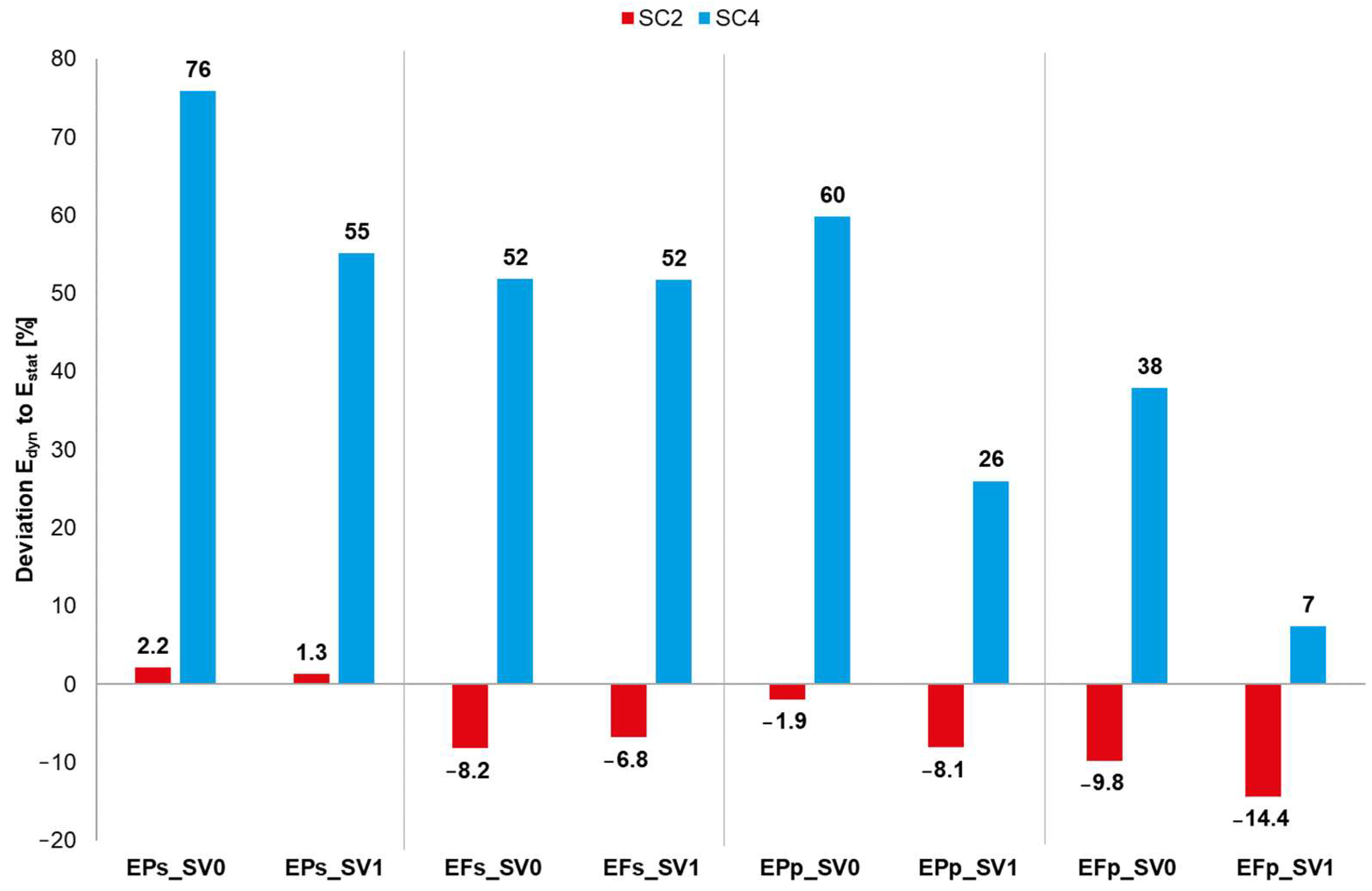
Figure 9 outlines these differences for SC2 and SC4 with a thermal and an electrical storage and an option PV system. System variant 1 (_SV1) represents the approach with the bigger capacity.
The answer to the third research question can be answered in two parts. First, the change in the storage characteristics only shows marginal effects on the emission balance using a simple load strategy. Secondly, there is a substantial impact on the energy balance when choosing a bigger storage capacity and a predictive load strategy. With extended loading periods, more advantageous load times can be used, which results in lower emissions.
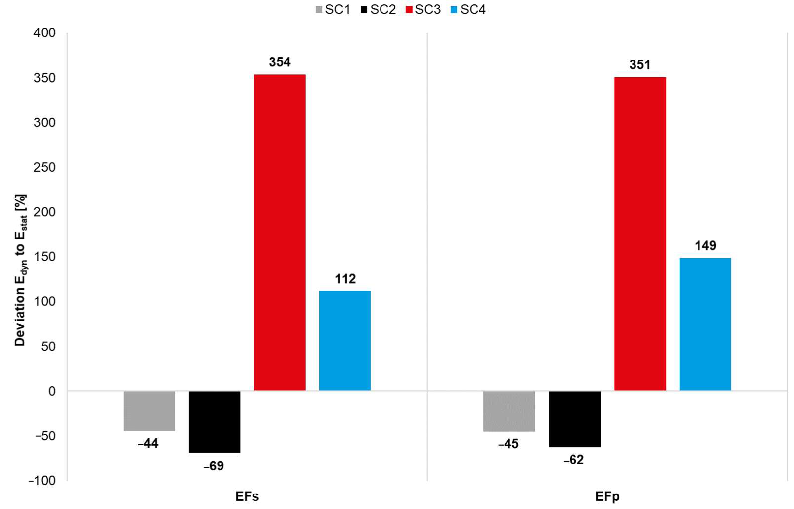
5.4. Impact of the Dynamic Emission Calculation for the Transformation of the German Electricity Grid
To evaluate the impact on the German electricity grid, a future scenario is analyzed that takes future electricity data into account. Thereby, only the effects on the emissions and the net load are analyzed, as a prediction of the future energy prices would be very imprecise.
The future scenario considers a huge expansion in the PV and wind energy that leads to a major reduction in the emission factor. Overall, the average emission of 2018 will be reduced from 469 to 62 g CO2/kWh in 2040. Within a 48 h prediction period, and in the future electricity grid, multiple minima often exist. To use these periods effectively, the concept of the centered moving average was applied. The detection of the minimum based on this concept, according to a self-defined threshold, was set to 50 g CO2/kWh. If the value of the considered period is higher than the threshold, the minimum is the center of the period. If the value is smaller than the threshold, the minima is set to noon.
The high reduction potential based on the lower emission factors is also represented in the deviation between the static and the dynamic approach. All deviations for all system configurations are bigger.
Figure 10 shows the difference between the static and the dynamic approach for the simple and predictive emission factor approach for SC1 to SC4. In SC1 and SC2, the simple approach shows slightly smaller negative deviations. For SC3, the deviations are bigger, whereas in SC4, the simple approach shows smaller differences. This leads back to the storage characteristics of the system and, with bigger storage, the advantages of the predictive approach would show these potentials (results not presented in this paper).
Even more so than with the emission balance, the net load mainly depends on the PV characteristics of the grid. The net load is defined as the ratio between consumption and production within the net. Overall, with predictive control in 2040, the net load is reduced by 18% in comparison to the average control, where this reduction in 2018 amounts to just 4%. The differences in the net load between the two predictive control strategies are marginal.
The answer to the fourth research question is divided into the impact on the emissions and the net load. In a future electricity grid with more regenerative energies, an emission-factor-based control can result in bigger savings. This is due to the huge daily fluctuation. It also results in bigger deviations between the static and dynamic approach for system configurations with PV. Already, simple-emission-based control strategies create emission savings in the summer period. To use the winter periods efficiently, predictive control is more suitable. Based on the dominance of PV in the future scenario, the indicator net load correlates with the emission-optimized controls. The differences between the individual control strategies are minor. Based on these findings, the authors suggest further research be performed focusing on a net-load-optimized control.
6. Discussion
The following provides a summarizing discussion of the most relevant outcomes of this study. The authors outline the main findings of the research questions and reprise the hypothesis. This chapter is divided into sections dealing with the localization, utilization, and transformation of the potentials of the dynamic emission factor. Finally, the limitations of this paper are outlined before giving an outlook.
The results of this paper attest to the statements of the hypothesis. The outcomes of the individual research questions prove this assertion. The potentials of the hourly dynamic emission factor are classified in the next three sections.
6.1. Location of the Potentials
Nowadays, emission factors play a key role in the evaluation of the sustainability of buildings. As of now and for reasons of convenience, only a static emission factor is considered for the energy balance. For certain system configurations, this can deliver comparable results to a dynamic approach. This is not the case for building systems with a PV system, a distinct storage system, or fluctuating user demands and emission factors. A PV system leads to higher overall balances, as the dynamic credit system is significantly smaller than the constant static one. Storage systems, especially with a heat pump or battery storage in combination with intelligent control strategies, open up huge potential to shift loads. In general, in an office environment, with or without mechanical ventilation, the dynamic approach can lead to emission savings due to the demand concentration in the midday hours.
6.2. Utilization of Potential
Using a predictive control strategy with storage systems creates significant emission savings. In the summer periods, simple load strategies already generate good results. In winter times, with fluctuating and irregular low-emission periods, predictive control strategies outperform simple ones. The increasing seasonality in regenerative productions, as well as the increasing fluctuating demands also in future scenarios, demands predictive control strategies to lower emissions in the best possible way.
This demand for predictive control strategies is also represented when extending the shifting periods with bigger storage systems. The results of this paper show that bigger storage systems only perform suitably with an emission-optimized predictive control strategy that leads to further emission savings.
6.3. Transformation of the Potential
The forecast scenario data of Agora Energiewende for the German electricity grid predicts a substantial increase in renewable energy, especially in photovoltaics. This leads to a general deviation between the static and dynamic approaches for all the system configurations. Furthermore, the emission savings due to the predictive control strategies and the increased storage systems go hand in hand with the demand concentration in the winter periods. In future summer periods, these advanced control strategies and the bigger storage do not result in a surplus of emission savings, as there are daily long periods of low emissions. In a future emission-neutral electricity grid, this rather demands an efficient way to handle the topic of the net load.
6.4. Limitations
The characteristic data of the emission factor only correlate partially with the real energy price and the net load of Germany’s electricity grid, and thus no full conclusions can be drawn. This further leads to the fact that the simulation variants with the lowest emissions are not necessarily linked to the lowest costs.
As outlined previously, the balance boundaries of this paper comprise the operation of a building. This means that this paper only outlines statements regarding various system configurations and does not evaluate the overall emission balance of a building. The findings of this paper only present tendencies when comparing the operation of different building technology systems.
Furthermore, the results are presumed with an efficient groundwater heat pump that uses electricity as the main energy source. Indeed, these systems are trendsetting but the outcomes of this paper are not necessarily applicable to other building technology systems.
The indicator net load in this paper only covers the ratio between net consumption and net production. With the increase in the fluctuation and the low-emission phases, the topic of timing the demand and supply is becoming essential but was not considered in this paper.
7. Conclusions
The complex topic of this paper results in a variety of assumptions and limitations that give rise to a multitude of further research topics. As the results present a promising outlook overall, the topic of a dynamic emission factor should be included in the process of thermal simulation in general, to evaluate the emission balance more precisely. This leads back to the previously mentioned topic of a holistic emission balance beyond the building operation and the impact of the dynamic emission factor. This also comprises the building technology components of, e.g., a heat pump, storage, or a PV system, and should be evaluated for the whole life cycle of a building.
To better represent the seasonality of the demand side, the daily profiles of the devices and the user should also vary over the course of the year. This would extend the fluctuation on the demand side and could increase the need for intelligent control strategies to balance the electricity grid.
The electrical energy generated by the photovoltaic system in this paper is directly transferred into the grid when no local consumers are available. In the case of battery storage, the concept of the immediate supply could be rethought to optimize the concept of a credit note.
This paper focuses on the German net and the location of Munich. Further research should include other national and international locations with different electricity grids and weather conditions. With these analyses, the concept of a dynamic emission factor could be brought in a broader discussion.
The practical significances of this paper is twofold. First, it shows that the general concept of analyze an emission balance needs to be reevaluated, and a dynamic emission factor should be mandatory for such analyses. Secondly, the developed control strategy should be used and implemented in existing buildings to reduce their emissions.
The results of this paper are based on a variety of assumptions, taking into account building characteristics, especially user and device profiles, as constant. These assumptions are based on conventional norms and codes, especially for lighting, heating, and ventilation. A broader view, such as the predictive control of these variables with the focus on energy efficiency and thermal comfort, could result in new possibilities. This has already been shown in initial research approaches using the building mass and its inert technology itself as energy storage with a further research approach looking into transforming buildings into short-term emission storage.
Author Contributions
Conceptualization, C.H., K.B., L.L., S.C.K. and T.A.; methodology, C.H., K.B. and L.L.; software, C.H., K.B. and L.L.; validation, C.H., K.B. and L.L.; formal analysis, C.H., K.B., L.L. and S.C.K.; investigation, C.H., K.B. and L.L.; resources, C.H., K.B., L.L., S.C.K. and T.A.; data curation, C.H., K.B. and L.L.; writing—original draft preparation, C.H. and K.B.; writing—review and editing, C.H., K.B., L.L., S.C.K. and T.A.; visualization, C.H., K.B. and L.L.; supervision, T.A.; project administration, C.H. All authors have read and agreed to the published version of the manuscript.
Funding
This research received no external funding.
Data Availability Statement
The data presented in this study are available upon request from the corresponding author.
Conflicts of Interest
The authors declare no conflict of interest.
Nomenclature
| Variable and parameters |
| Level of efficiency at 25 °C (STC) | (-) |
| Irradiation on solar panel | (W/m2) |
| e | Euler’s number | (-) |
| a, b, c | Model parameters | (-) |
| Level of efficiency | (-) |
| Temperature of solar panel | (°C) |
| Temperature efficiency | (-) |
| PV power | (W) |
| Surface area of solar panel | (m2) |
| Level of efficiency of inverter | (-) |
| Level of efficiency of mismatching | (-) |
| Level of efficiency of cable | (-) |
| Level of efficiency of spectral | (-) |
| Total CO2 emission dynamic | (kg CO2) |
| Total CO2 emission static | (kg CO2) |
| Power provided by the net | (kWh) |
| Hourly emission factor | (gCO2/kWh) |
| Average emission factor over year | (kg CO2) |
| Total electricity costs | (EUR) |
| Domestic electricity price | (EUR/kWh) |
| Total net load | (kWh) |
| Percentage of net load per hour | (-) |
| Abbreviations |
| EF | Emission factor | |
| PV | Photovoltaics | |
| GeG | Gebäudeenergiegesetz—German Building Energy Code | |
| DWD | Deutscher Wetter Dienst—German Weather Forecast Service | |
| COP | Coefficient of performance | |
| SC | System configuration | |
| SV | System variant | |
| Eps | Energy price simple | |
| EPp | Energy price predictive | |
| EFs | Emission factor simple | |
| EFp | Emission factor predictive | |
References
- United Nations. Framework Convention on Climate Change. In Proceedings of the Adoption of the Paris Agreement, 21st Conference of the Parties, Paris, France, 30 November–11 December 2015. [Google Scholar]
- UNEP. 2020 Global Status Report for Buildings and Construction: Towards a Zero-emission, Efficient and Resilient Buildings and Construction Sector; United Nations Environment Programme: Nairobi, Kenya, 2020. [Google Scholar]
- ISE. Wege zu einem klimaneutralen Energiesystem—Die deutsche Energiewende im Kontext gesellschaftlicher Verhaltensweisen; Fraunhofer-Institut für Solare Energiesysteme ISE: Freiburg, Germany, 2020. [Google Scholar]
- BMU: Bundesministerium für Umwelt, Naturschutz, nukleare Sicherheit und Verbraucherschutz 2020, Klimaschutzbericht; DMUB: Bonn, Germany, 2020.
- GEG: Gebäudeenergiegesetz. Bundesnetzgesetzblatt Jahrgang 2020 Teil I Br. 37; Bundesanzeigerverlag Bundesgesetzblatt: Bonn, Germany, 2020. [Google Scholar]
- Regett, A.; Heller, C. Relevanz zeitlich aufgelöster Emissionsfaktoren für die Bewertung tages- und jahreszeitlich schwankender Verbraucher. Energ. Tagesfr. 2015, 65, 46–50. [Google Scholar]
- Seckinger, N.; Radgen, P. Dynamic Prospective Average and Marginal GHG Emission Factors—Scenario-Based Method for the German Power System until 2050. Energies 2021, 14, 2527. [Google Scholar] [CrossRef]
- Wörner, P.; Müller, A.; Sauerwein, D. Dynamische CO2-Emissionsfaktoren für den deutschen Strom-Mix. Bauphysik 2019, 41, 17–29. [Google Scholar] [CrossRef] [Green Version]
- Müller, A.; Wörner, P. Impact of dynamic CO2 emission factors for the public electricity supply on the life-cycle assessment of energy efficient residential buildings. IOP Conf. Ser. Earth Environ. Sci. 2019, 323, 1–9. [Google Scholar] [CrossRef]
- DWD Klimadaten Deutschland—Stundenwerte (Archiv). 2021. Available online: https://www.dwd.de/DE/leistungen/klimadatendeutschland/klarchivstunden.html (accessed on 24 October 2021).
- Hepf, C.; Schmid, S.; Brunet, F.; Auer, T. Validation of Thermodynamic Building Model Based on Weather and Thermal Measurement Data; BauSIM: Weimar, Germany, 2022; pp. 189–195. [Google Scholar]
- Agora. Klimaneutrales Deutschland 2045—Wie Deutschland seine Klimaziele schon vor 2050 erreichen kann—Langfassung; Agora Energiewende: Berlin, Germany, 2021. [Google Scholar]
- Solar Energy Laboratory, University of Wisconsin. TRNSYS 18 A TRaNsient System Simulation Program; Standard Component Library: Madison, WI, USA, 2017. [Google Scholar]
- Ladybug Tools LLC Honeybee. 2022. Available online: https://www.ladybug.tools/honeybee.html (accessed on 6 October 2022).
- Jocher, T.; Loch, S. Raumpilot Grundlagen; Wüstenrot Stiftung: Ludwigsburg, Germany, 2012. [Google Scholar]
- DIN—Normenausschuss Baulicher Wärmeschutz im Hochbau; DIN-Normenausschuss Bauwesen (NABau). DIN 4108—Wärmeschutz und Energie-Einsparung in Gebäuden; Beuth Verlag GmbH: Berlin, Germany, 2013. [Google Scholar]
- DIN—Normenausschuss Baulicher Wärmeschutz im Hochbau; DIN-Normenausschuss Bauwesen (NABau). DIN V 18599-10, Energetische Bewertung von Gebäuden—Berechnung des Nutz-, End- und Primärenergiebedarfs für Heizung, Kühlung, Lüftung, Trinkwarmwasser und Beleuchtung—Teil 10: Nutzungsrandbedingungen, Klimadaten; Beuth Verlag GmbH: Berlin, Germany, 2018. [Google Scholar]
- DIN—Normenausschuss Baulicher Wärmeschutz im Hochbau; DIN-Normenausschuss Bauwesen (NABau). DIN EN 16798-1 Energetische Bewertung von Gebäuden—Lüftung von Gebäuden—Teil 1: Eingangsparameter für das Innenraumklima zur Auslegung und Bewertung der Energieeffizienz von Gebäuden bezüglich Raumluftqualität, Temperatur, Licht und Akustik; Beuth Verlag GmbH: Berlin, Germany, 2019. [Google Scholar]
- Heydenreich, W.; Büller, B.; Reise, C. Describing the world with three parameters: A new approach to PV module power modelling. In Proceedings of the 23rd European Photovoltaic Solar Energy Conference and Exhibition, Valencia, Spain, 1–5 September 2008; pp. 1–4. [Google Scholar]
- Weniger, J.; Quaschning, V.; Tjaden, T. Optimale Dimensionierung von PV-Speichersystemen. PV Magazine, January 2013, pp. 70–75.
| Publisher’s Note: MDPI stays neutral with regard to jurisdictional claims in published maps and institutional affiliations. |
© 2022 by the authors. Licensee MDPI, Basel, Switzerland. This article is an open access article distributed under the terms and conditions of the Creative Commons Attribution (CC BY) license (https://creativecommons.org/licenses/by/4.0/).


