Valuation of Land-Use/Land-Cover-Based Ecosystem Services in Afghanistan—An Assessment of the Past and Future

Abstract

Being one of the weakest economies in the world, livelihoods in Afghanistan remain highly dependent on local ecosystem services. However, the risk of ecosystem services degradation in Afghanistan over the past two decades has significantly increased, mainly due to rapid changes in land-use and land-cover (LULC). As such, policy makers must be able to estimate the impact of LULC changes on various ecosystem services. By utilizing GlobeLand30 land cover products for 2000, 2010 and 2020, and by adopting the value transfer method, this study assessed the ecosystem services value (ESV) changes in response to the changes of LULC in Afghanistan. Additionally, the dynamics of the land system (DLS) model was innovatively coupled with linear programming to predict likely scenarios of ESV changes by 2030. The predicted results were also validated against actual land cover and achieved a Kappa value of 0.78. The results showed that over the 20-year period, ecologically important LULC categories such as forest, water bodies and grassland were severely unstable and rapidly decreasing in scope. These LULC types were being threatened by agricultural, built-up and unused lands. During this period, we estimated a decrease in the total ESV from 161 billion USD in 2000 to 152.27 billion USD in 2020. About 92% of this decrease was shared by supporting and provisioning services. The simulated scenarios also showed that ESV will likely further decrease under Business-As-Usual (BAU), and Rapid Economic Development (RED) scenarios. Positively, an Environmental Protection (ENP) scenario is predicted, with a 4.5% increase in ESV by 2030. However, achieving this scenario requires the enforcement of strict environmental protection measures.

1. Introduction

Ecosystems are life-supporting systems and the foundation of human socioeconomic development. Through their functions, they provide various services which are essential for livelihoods and social welfare [1,2,3,4]. These services are broadly categorized into “direct affecting”, e.g., regulating, provisioning services, and cultural and “indirect affecting”, e.g., supporting services [5,6]. However, the dynamics of land-use and land-cover (LULC) can directly affects the status, integrity and supply of ecosystem services [7,8]. While a heavily human-managed land system is able to meet various human needs, its excessive usage disturbs ecological processes, affecting its capacity to remain productive [9]. In the recent past, the pace and intensity of LULC change have been exacerbated by growing human activities [10].

During the past few decades, the rapid growth of the population and socioeconomic development have accelerated urban and agricultural sprawl globally, encroaching upon natural landscapes such as forest and grasslands [11,12]. A study by Robertson and Swinton [13], for instance, revealed that globally, each year, about 13 million ha of land is added for agriculture, mainly encroaching on woodland areas. Such rapid conversion of ecologically important landscapes has severely impacted biodiversity and reduced the capacity of ecosystems to serve future generations [14,15,16,17]. In fact, the additional gains generated from the conversion of natural landscapes to production-oriented lands comes with the cost of declining ecosystem services [18]. It is estimated that over the past 50 years, nearly 60% of ecosystem services have degraded [5].

Policy makers in the recent past have paid particular attention to the question of how to minimize the adverse effects of rapid socioeconomic development on the supply of ecosystem services. Communicating changes in ecosystem services in monetary value offers a globally accepted measure that can meet the needs of policy makers [19,20,21]. However, we are faced with a major challenge, i.e., how to communicate the economic effect of the ecosystem service changes, since most of the supplied services are not captured by market values [22,23,24]. Therefore, accurate estimations of the spatiotemporal changes of ecosystem services remain difficult.

Broadly, at least four major approaches to ecosystem services valuation (ESV) are found in the existing literature [25]. They include the benefits transfer approach, stated preference approaches such as the contingent valuation method, cost-based approaches such as the replacement cost and avoided cost methods, and revealed preference approaches such as the travel cost and market prices methods [26]. Amongst these methods, the benefits transfer method (BTM) is an easy to apply approach that uses a given valuation study to assess a new location of similar characteristics [26].

Over the past two decades, this method has been applied to a wide range of environmental studies, from forest management [27] to water quality and health risks [28,29], as well as waste management [30]. Likewise, the research of Costanza, d’Arge, De Groot, Farber, Grasso, Hannon, Limburg, Naeem, O’neill and Paruelo [4], for the first time, applied BTM to assess the monetary value of 17 ecosystem services provided by 16 global landscapes. Later, these estimates were further updated by conducting more than 300 case studies across various region of the globe [16,22]. Most importantly, this research provided a basis for utilizing estimates and the model in other regions. As a result, many researchers have used this approach and assessed the impact of LULC changes on ecosystem services [21,31]. Under this approach, changes in the supply of ecosystem services were investigated by considering LULC changes as an alternative to the supply of ecosystem services [12,22,24,32,33,34,35,36,37,38,39]. However, much of the research which has utilized the Costanza, d’Arge, De Groot, Farber, Grasso, Hannon, Limburg, Naeem, O’neill and Paruelo [4,22] coefficients considered changes of the physical supply of ecosystem services only.

Some later studies, therefore, argued that the value of services is not only affected by quantity changes in supply, but also by the simultaneous changes of demand of goods and services [21,40,41]. For this reason, in their study, Bryan, Ye and Connor [21] proposed a more complex methodology that incorporates the scarcity effect of supply and demand into the Ye, et al. [42] model of constant coefficients. Scarcity refers to limitations of ecosystem services that increase the willingness of consumers to pay high prices, which may significantly impact valuations of ecosystem services [21]. The effect of scarcity is particularly crucial for land types that are prone to high demand and supply changes, such as a built-up areas. However, this methodology depends on the availability of specific economic indicator data which may not be available for some regions for the required period. Also, the LULC quality effect, which may change over time and can alter the ecosystem services supply capacity. Some recent research has used the vegetation index to address regional capacity differences of land use in terms of the provision of ecosystem services. A study by Fei, et al. [43], Xie, et al. [44] for instance, incorporated the net primary productivity (NPP) of natural vegetation into constant coefficients to account for regional capacity differences in the supply of ecosystem services. The effect of vegetation quality is particularly significant in natural land use types such as forests and water bodies.

Ecosystem services in Afghanistan are also of particular importance and urgently require the attention of policy makers to protect their supply capacity in the face rapid socioeconomic development. Due to weak industrial growth, the livelihoods of nearly 80% of the Afghan population are directly or indirectly supported by the local ecosystem [45]. Furthermore, agroecosystem services alone provide jobs to about 40–60% of the labor force and contribute to one-fourth of the gross domestic product (GDP) [46,47]. Similarly, grasslands and forests support local livelihoods by protecting soils and water for agriculture and providing goods and services for energy, construction, and other sectors [48]. For instance, grassland occupies about 47% of country’s land and supplies about three quarters of the livestock fodder [48]. Likewise, forests cover nearly 2% of the total land area in Afghanistan; these areas produces internationally valued timber and non-timber products [49]. Moreover, rangeland and forestlands prevent natural disasters and safeguard locals from socioeconomic damages [50]. However, despite their enormous economic benefits, ecosystem services have been traditionally undervalued by decision makers, mainly due to a lack of knowledge and poor-quality research [49]. In Afghanistan, ESV is even more important in the face of four decades of continuous instability that has damaged the structure and functioning of ecosystem [45,51]. The crisis grows further as rapid population growth, particularly after 2000, and deteriorating climatic conditions are adding to the pressure on ecosystem. Currently, of the identified ecoregions in Afghanistan, 38% of all land areas are classified as endangered and another 61% are as vulnerable [52]. Likewise, nearly 70% of woodland areas in Afghanistan have been identified as vulnerable [52]. Satellite evidence has revealed that forests in many areas are in the brink of disappearance.

Besides the aforementioned issues, it is also important to understand the changes of ecosystem services due to huge foreign investment during the period in which the USA and allied countries were present in Afghanistan. Upon the fall of Taliban regime in 2002, the newly formed government received ample foreign funds for environmental restoration and economic development. During the period of 2002–2021, the USA-supported Afghan government implemented many long- and short-terms plans to achieve the given goals. For instance, as an economic development strategy, the National Peace and Development Framework (ANPDF) offered various national priority programs to accelerate GDP growth from 0.9% in 2015 to 5.7% in 2030; and expand stable irrigated land to the pre-war level of 3.1 million ha [46,53]. Similarly, as an environmental restoration strategy, it was planned to restore 60,000 ha of deforested land in every five years [46,53].

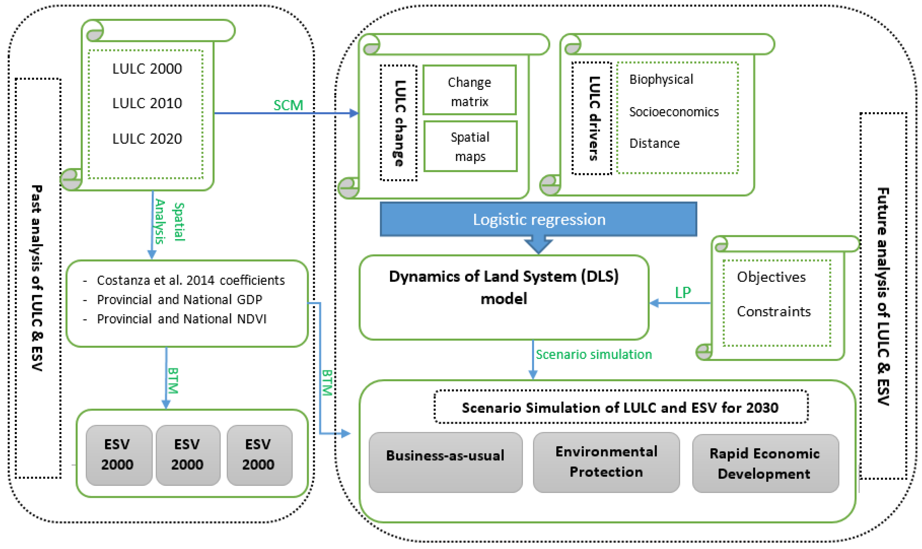
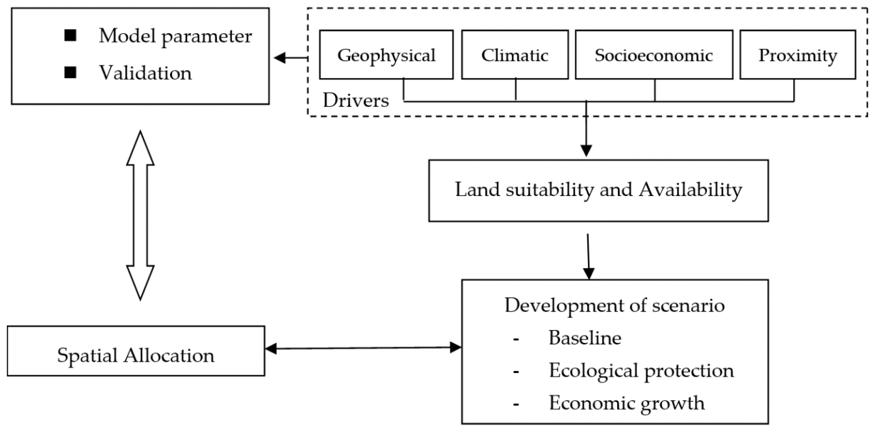
Although some studies have attempted to trace the trends and drivers of LULC change in various small regions in Afghanistan [54,55,56,57,58,59], nationwide studies are still lacking. The approaches adopted by some studies were also questionable. Most importantly, to our knowledge, impact assessments of the aforementioned changes on ESV (in monetary values) in Afghanistan are completely lacking. This study, therefore, aimed to fill this research gap. Firstly, we set out to utilize the 30 m resolution land cover product from GlobeLand30 to estimate the monetary values of ecosystem services in relation to LULC changes in Afghanistan between 2000, 2010, and 2020. Secondly, we sought to establish rational scenarios and simulate future LULC and ESV for 2030. For this purpose, as both scarcity and LULC quality effects are crucial to the provision of ecosystem services, our study adopted the methodology proposed by Fie, et al. [43] to assess ecosystem service changes in Afghanistan.

The significance of this study is twofold. Firstly, such quantitative assessments are urgently needed in the data-scarce region of Afghanistan, where human-induced environmental degradation is accelerating [51,60]. Secondly, the study innovatively couples linear programming with LULC simulation modeling to develop more rational scenarios. Our assessment of the supply of future ecosystem services under various rational scenarios is particularly important for the creation of suitable policy measures in LULC management. Most ecosystem service valuation studies have largely focused on spatiotemporal trends and ignored future change under national policy scenarios which are relevant to LULC. Some studies from elsewhere have applied LULC simulation models to predict ESV at small scales [21,43,56]. However, the creation of logical scenarios of future land-use change remains a challenging task in the literature. Except for the business-as-usual scenario, which explains the status quo, the land allocation process under other scenarios remains ambiguous and mostly based on researchers’ judgement. In this study, a more logical scenario development process is used, i.e., defining future objectives and identifying the constraints on the achievement thereof. This is crucial, because the rationalization of object and constraint functions provides the luxury of utilizing linear programming to estimate future land allocations in land-use simulation modeling, instead of depending on human judgment.

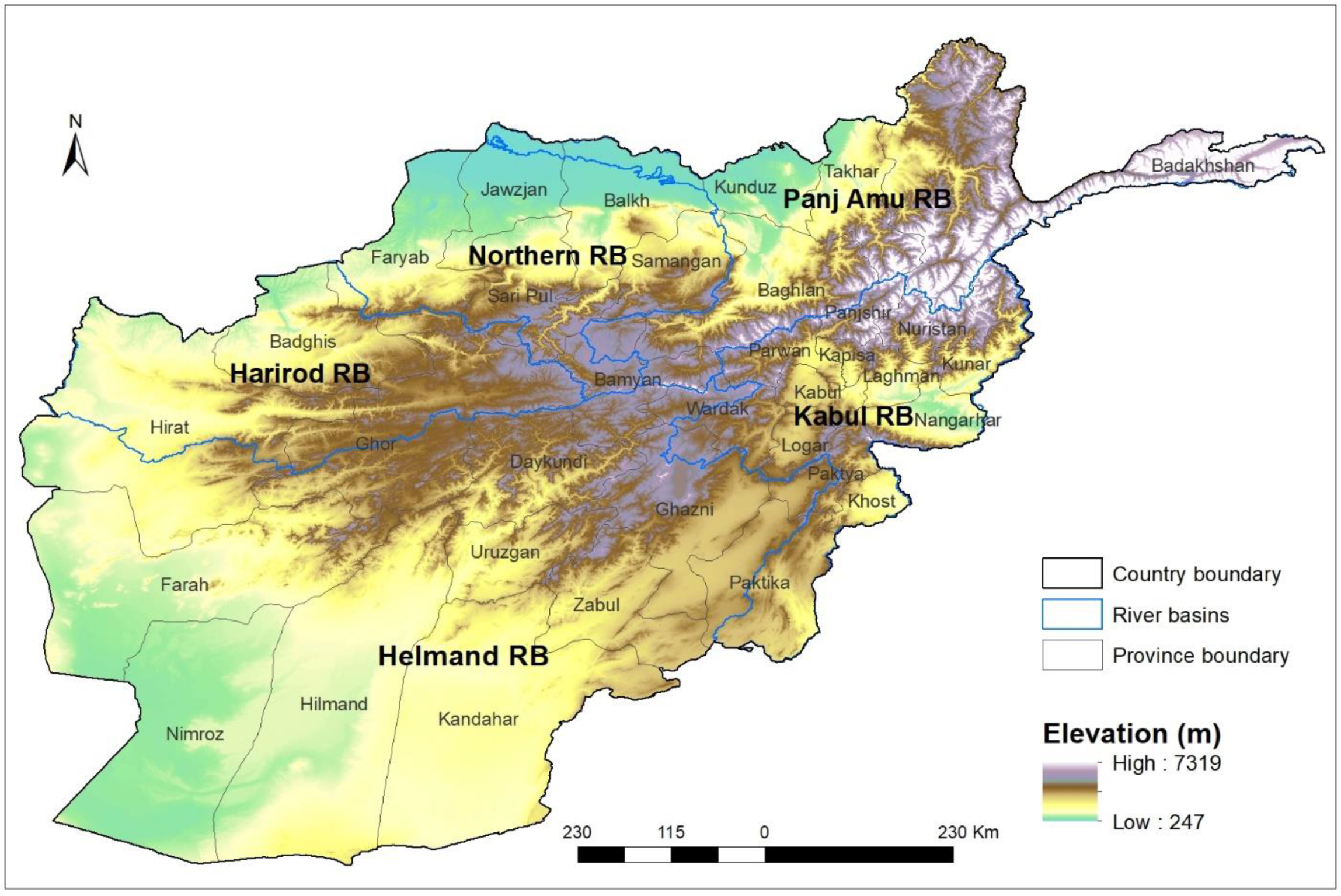
Establishing such functions for this study is significant because, in Afghanistan, maximizing value benefits from ecosystem services by enhanced land-use management is hindered by major constraints such as water scarcity, limited financing, and access to productive lands. Afghanistan is located in a semi-arid region, where a reliable, timely, and sufficient water supply for agricultural, environmental, and industrial uses remains challenging. Limited access to water resources has traditionally constrained the attainment of economic and environmental goals [61]. In many areas, for instance, water scarcity has forced farmers to leave nearly one-third of their cultivated land fallow [47,62,63]. Similarly, land has an economic value that can play a significant role in achieving economic growth [64,65]. Land in Afghanistan is particularly scarce; the overall terrain is dominated by dry craggy mountains, which leaves only 12–15% for natural vegetation and economic activities [46]. Besides water and land scarcities, financial capital is also significantly limited for the implementation of economic and environmental development programs. Afghanistan is one of the poorest economies in the world, and its development budget is hugely dependent on foreign funding. Currently, the announced budget for 2022 under the Taliban government is faced with a 20% budget deficit [66].

2. Materials and Methods

2.1. Study Framework

Figure 1 explains the general framework of this study. Broadly, this research is divided into two directions, i.e., (1) past and (2) future assessments of LULC-induced ESV changes. The past trends analysis was conducted with the primary objective of estimating the value changes of ecosystem services between 2000, 2010, and 2020. For this purpose, the study adopted the BTM approach and utilized Globland30 high resolution LULC data (for 2000, 2010 and 2020), the coefficients of [22], and GDP and NDVI information. This process allowed us to make estimations of ESV for 2000, 2010 and 2020.

The second part of this study was guided by the objective of assessing various possible future scenarios of ESV change in Afghanistan. Here, we first conducted a LULC cover change analysis by using actual LULC data and applying the Special Calculation Model (SCM) and change matrix analysis. The outputs of this analysis were spatial change maps and a change matrix (transition matrix). The spatial change maps were coupled with spatial layers of hypothesized LULC change drivers to conduct a regression analysis. Statistically significant coefficients were then used as the inputs for the Dynamic Land System (DLS) model. Similarly, the transition matrix and the results of Linear Programming (LP) of objective and constraint functions were used to allocate pixels of various LULC types under the identified scenarios. Based on this analysis, we allocated LULC types in DLS modeling. The final outputs of the DLS modeling were spatial maps of LULC for 2030 under BAU, ENP, and RED scenarios. Finally, we once again used the BTM approach and predicted ESV for 2030 from the simulated LULC maps.

2.2. Study Area

The study area covers the entirety of Afghanistan, a landlocked country which is located in a semi-dry region. It shares borders with Iran in the west, Pakistan in the east and south, China and Tajikistan in the northeast, Uzbekistan in the north and Turkmenistan in the northwest (Figure 2). Administratively, Afghanistan is divided into 34 provinces and 365 districts. In terms of hydrological topography, Afghanistan shares five major river basins, namely, the Amu Darya basin, the Helmand basin, the Kabul (Indus) basin, the Harirod-Morghab basin, and the Northern basin. Altitude in Afghanistan varies from high Hindu Kush Mountains in the north to the plain deserts in the south. Although it is an agriculturally dependent country, 65% of Afghanistan’s land is covered by mountains, with only 12% of its total area being arable land.

The highly variable topography in Afghanistan results in significant climatic variation. For instance, the temperature ranges from about −50 °C in winter in the northern high mountains to about +50 °C in the summer in the southern deserts. Winter snowfalls are actually the origin of life-supporting river systems that flow across the five aforementioned river basins [61]. The spatiotemporal distribution of precipitation also varies amongst the regions. Overall, Afghanistan is a dry country with marginal annual rainfall. However, the level of dryness changes from one region to another [67,68]. In contrast to other regions, the eastern area is characterized by a semi-monsoon climate that provides the basis for forest cover in the country [69,70]. Such climatic variation affects the vegetation cover significantly [67], which subsequently affects the supply of ecosystem services [43,71,72,73].

Likewise, over the past two decades Afghanistan has experienced immense socioeconomic changes which may have disturbed the supply–demand balance of ecosystem services, as indicated elsewhere [21,40]. During the period in which the USA and allied nations were present in Afghanistan, GDP increased from 8689 million US dollars in 2003 to 21,969 million US dollars in 2017 [60]. However, this economic growth was characterized by regional variations that were evidenced by increasing the Gini-coefficient [74]. Similarly, according to World Bank data, Afghanistan’s population has grown from about 22 million in 2002 to about 38 million in 2020 [75,76].

2.3. Data Preparation

This study utilized LULC, climatic, socioeconomic, and biophysical data to achieve its research objectives. Most of the obtained datasets were utilized for the purpose of identifying the drivers of change (regression analyses) in the LULC simulation process. Furthermore, this research required all the datasets in spatial raster format. Tabulated GDP data were preferred over global datasets to minimize errors. The interpolation functions of the geographical information system (GIS) were applied to convert tabulated data into the required gridded format [77]. As LULC data were the main source utilized for ESV estimates, their accuracy and resolution were crucial to obtain accurate results. Therefore, amongst the publicly available datasets, the Globland30 LULC product was selected for this research. It is a 30 m high resolution LULC dataset which is available for the years 2000, 2010 and 2020. This global LULC product was developed using various satellite images, such as Landsat TM/ETM+ and HJ-1 imagery, and adopting a pixel-object-knowledge (POK)-based classification approach [78,79]. Globland30 products have been shown to have good overall average accuracy and a kappa coefficient of 82% and 0.80, respectively [80,81]. Brief details of the datasets that were used in the regression analysis are provided in the

Table 1. Description of the datasets used in this study.

Dataset	Description	Source/Download link
LULC	Land-use land-cover	[79]/www.globeland30.org (accessed on 12 February 2022)
ET	Actual evapotranspiration (mm)	[82]/www.ntsg.umt.edu (accessed on 12 March 2021)
Elevation	Derived from digital elevation model (DEM)	[83]/Earthdata|Earthdata (nasa.gov)
Slope	Area lope derived from DEM (degree)	[83]/Earthdata|Earthdata (nasa.gov)
Soil pH	pH value	[83]/SoilGrids250m 2.0
Soil Density	Soil density (g/cm3)	[83]/SoilGrids250m 2.0
Temperature	Average annual temperature (°C)	[84] https://crudata.uea.ac.uk/cru/data/hrg/ (accessed on 5 January 2022)
Precipitation	Average annual rainfall (mm)	[84] https://crudata.uea.ac.uk/cru/data/hrg/ (accessed on 5 January 2022)
Population density	Person/Km2	[85]/www.worldpop.org.uk (accessed on 12 February 2022)
GDP	$/person	[86]/cso.gov.af (accessed on 12 March 2021)
Irrigation expansion investment	$ required for expansion of Km2 irrigated	[86]/cso.gov.af (accessed on 12 March 2021)
Province capital coordinates	Distance of pixels to the closest city	Google Earth
Main roads	Distance of pixels to the closest road	[87]/www.diva-gis.org (accessed on 12 March 2021)
NDVI	Vegetation cover	[82]/www.ntsg.umt.edu (accessed on 12 March 2021)

.

2.4. Analytical Tools

2.4.1. LULC Change Analysis of Afghanistan

LULC change between 2000 and 2020 was estimated using the spatial calculating model (SCM) [88].

$$L{U}_i=\left(\frac{\left(L{A}_{\left(i,t1\right)}-UL{A}_i\right)+\left(L{A}_{\left(i,t2\right)}-UL{A}_i\right)}{L{A}_{\left(i,t1\right)}}\right)·\frac{1}{T_2-T_1}·100\%$$

(1)

where LU_i is the percentage change of ith LULC between T₁ and T₂; T₁ and T₂ are years 2000 and 2020, respectively; $L{A}_{\left(i,t1\right) }$ and $L{A}_{\left(i,t2\right)}$ represent the area of i_th LULC type in t₁ and t₂, respectively; and $UL{A}_i$ is the unchanged area of i_th LULC type during this period.

The directions of change were analyzed by developing a change matrix of six LULC types. Using GIS functions, the pixels of a LULC type which changed to another LULC type between the study years were assessed, and the following matrix was developed:

$$\left[\begin{array}{cccccc}L{C}_{AgAg}& L{C}_{AgFr}& L{C}_{AgWb}& L{C}_{AgWb}& L{C}_{AgBl}& L{C}_{AgUl}\\ L{C}_{FrAg}& L{C}_{FrFr}& L{C}_{FrGr}& L{C}_{FrWb}& L{C}_{FrBl}& L{C}_{FUl}\\ L{C}_{GrAg}& L{C}_{GrFr}& L{C}_{GrGr}& L{C}_{GrWb}& L{C}_{GrBl}& L{C}_{GrUl}\\ L{C}_{WbAg}& L{C}_{WbFr}& L{C}_{WbGr}& L{C}_{WbWb}& L{C}_{WbBl}& L{C}_{WbUl}\\ L{C}_{BlAg}& L{C}_{BlFr}& L{C}_{BlGr}& L{C}_{BlWb}& L{C}_{BlBl}& L{C}_{BlUl}\\ L{C}_{UlAg}& L{C}_{UlFr}& L{C}_{UlGr}& L{C}_{UlWb}& L{C}_{UlBl}& L{C}_{UlUl}\end{array}\right]$$

(2)

where LC is LULC, Ag is agricultural land, Fr is forest area, Gr is grassland, Wb is water bodies, Bl is built-up land, and Ul is unused land.

2.4.2. Estimate of ESV

This study adopted the BTM approach to assign economic values to each of the nine services derived from land surface ecosystem. The method was based on ascribed coefficients (published by [22]) that represent the relative economic value of ecosystem services derived from the various land-types (

Table 2. The adopted coefficients [22] (US$ ha⁻¹ yr⁻¹) for an ecosystem service valuation (ESV) of similar LULC types in Afghanistan.

Type	Sub Type	AG	FR	GR	WB	BL	UL
Provisioning	Food production	2323	200	1192	106	0	0
	Raw materials	219	84	54	0	0	0
Regulating	Gas regulation	0	12	9	0	0	0
	Climate regulation	411	2044	40	0	0	0
	Disturbance regulation	0	66	0	0	0	0
	Water regulation	0	8	3	7514	0	0
	Water supply	400	27	60	1808	0	0
	Waste treatment	397	120	75	918	0	0
Supporting	Erosion control	107	337	44	0	0	0
	Soil formation	532	14	2	0	0	0
	Nutrient cycling	0	3	0	0	0	0
	Pollination	22	30	35	0	0	0
	Biological control	33	11	31	0	0	0
	Habitat/refugia	0	39	1214	0	0	0
	Genetic resources	1042	1517	1214	0	0	0
Recreation and culture	Recreation	82	867	26	2166	0	0
	Cultural	0	2	167	0	0	0
Total Ecosystem Value		5568	5381	4166	12,512	0	0

) [21].

The authors of [22] estimated the ESV coefficients for the 16 globally identified biomes. The coefficients of six identified biomes were used in our study as equivalents to the six LULC types in Afghanistan. We used agricultural land as an equivalent of cultivated land, forestland as an equivalent of forestland, grassland as an equivalent of grasslands and shrublands, urban land as an equivalent of built-up land, and desert/tundra/ice and rock as an equivalent of unused land.

However, the use of these coefficients to determine the ecosystem service value per unit of land is inappropriate if the study area specification is ignored. Therefore, we incorporated the NDVI and GDP information of the study area to adjust the coefficients for our ecosystem service valuation of the study area, as also done elsewhere [43]. Therefore, ESV was calculated by the following equation:

$$ES{V}_t=\sum \left(A_{it}\times V{C}_i\times R\times A\right)$$

(3)

where ESV_t represents the total ESV in year t, A_it represents the area of LULC type i in t, VC_i represents the ESV coefficient (US$ ha⁻¹ yr⁻¹) of the given i type LULC, and R represents the landscape quality effect on the supply of ecosystem services, which is calculated as follows:

$$R=\frac{NP{P}_{Pr}}{NP{P}_{Af}}$$

(4)

where NPP_Pr and NPP_Af represent the net primary productivity of a province and all of Afghanistan, respectively. NPP was estimated using the Thornthwaite Memorial model, which considers a comprehensive set of environmental factors [89]. The formula of the Thornthwaite Memorial model is as follows:

$$NPP=3000[1-e^{-0.0009695\left(V-20\right)}$$

(5)

$$V=\frac{1.05Pre}{\sqrt{1+{\left(1+\frac{1.05Pre}{L}\right)}^2}}$$

(6)

$$L=300+25Tmp+0.05Tm{p}^3$$

(7)

where NPP represents the net primary production potential of the natural landscape (t/ha/a), V represents evapotranspiration (mm/year), L represents annual mean evapotranspiration (mm), Tmp represents annual average temperature ($°$C), and Pre represents annual precipitation (mm)

In Equation (3), A represents the demand change effect on ESV, which is calculated as follows:

$$A=\frac{GD{P}_{Pr}}{GD{P}_{Af}}$$

(8)

where GDP_Pr and GDP_Af represent the per capita GDP (USD/person) of a province and of all of Afghanistan, respectively.

2.4.3. LULC and ESV Simulation with the DLS Model

To predict the future scenario of ESV changes in Afghanistan, we first simulated the LULC change for 2030 and then predicted ESV for the same year. The LULC of 2010 and 2020 were taken as the baseline data and incorporated into the DLS model. DLS is a land-use simulation model that combines a group of functions to predict future LULC changes based on information about the actual LULC, about driving factors and about established scenarios. It has two main favorable features: (1) it applies a dual stagey to reach a demand balance, and (2) in incorporates driving factors into the simulation process [90]. Hence, simulations with the DLS model include scenario development and analyses of specific driving factors of the study area.

The DLS framework includes three main modules (Figure 3). The first concerns the spatial regression modeling through which DLS integrates the variability of various driving factors and establishes the relationship of a piece of land with its driving factors. The second module concerns scenario analyses; this helps DLS to create demands for various LULC. The final module is a spatially explicit allocation module which allocates land use changes from regional to pixel level based on information from regression and scenario analyses. The predicted LULC maps can be validated against the actual LULC, which can also feedback the selection of variables.

Regression Analysis

Regression modeling was conducted to identify the driving forces of LULC change in Afghanistan. The coefficients of statistically significant LULC change drivers were required as DLS input parameters for LULC prediction. For this, various LULC change drivers were hypothesized to have significant impacts on LULC change. These variables were selected based on previous studies [55,91,93,94,95]. The hypothesized variables were then tested for significance using binomial logistic regression (BLR) [91,96]. The formula of BLR is as follows:

$$Y={\beta }_0+{\beta }_1{x}_1+{\beta }_2{x}_2+{\beta }_3{x}_3+\dots +{\beta }_n{x}_n+$$

(9)

where Y is the likelihood of a pixel of land changing to a LULC type due to the influence of driving factors x, x₂,..., x_n, and β₁, β₂,..., β_n are the coefficients of independent variables, while β₀ is a constant.

Table 3. Statistical description of the coefficients of influencing factors of land.

Driving factors	Agricultural	Forest	Grassland	Water	Built-Up	Unused
Temperature	−0.072 *	0.40 *	−0.05 *	0.02	−0.56 *	0.03
Precipitation	0.005 *	0.05 *	−0.01 *	0.03 *	−0.04 *	−0.01 *
Soil pH	−0.08 *	−0.41 *	0.02 *	0.16 *	0.16 *	0.10 *
Soil density	0.06 *	0.01 *	0.01 *	0.01 *	0.18 *	−0.01 *
Elevation	−0.03 *	−0.01 *	0.01 *	0.01 *	−0.01	0.01 *
Slope	−0.04 *	0.03 *	0.04 *	−0.03 *	−0.16 *	−0.04 *
Road distance	−0.03 *	0.01 *	−0.01 *	0.01 *	−0.01 *	0.01 *
City distance	−0.01 *	−0.01 *	−0.01 *	0.01 *	−0.01 *	0.01
Invest on irrigation	0.01 *	−0.06 *	−0.01 *	0.06 *	0.07 *	0.01 *
GDP/capita	−0.01 *	−0.01 *	−0.01 *	0.01 *	0.01 *	0.01 *
Population	−0.04 *	−0.01 *	−0.01 *	0.01	0.01 *	−0.01 *
AUC	0.83	0.84	0.78	0.76	0.76	0.80

Note: t statistics in parentheses: * p < 0.05.

shows the regression coefficients that were achieved by conducting BLR analysis. The negative coefficients indicate that a unit increase of a given independent variable may decrease the portability of an area change to a LULC type. On the other hand, positive coefficients show that a unit increase of a given independent variable increases the probability of an area being changed to a LULC type. For instance, the positive coefficient of precipitation under the agricultural land column suggests that a unit increase in rainfall will increase the probability of land being changed to agricultural area, while the negative coefficient of temperature in the same column explains the opposite. Although each coefficient requires detailed discussion and reasoning, we avoid this discussion as it is not relevant to the main objective of this research. Nonetheless, two features of the regression table should be mentioned here. Firstly, most of the regressed independent variables were statistically significant, which indicates that most of the hypothesized factors had the ability to explain land-use spatial allocation. Secondly, the values of the areas under the ROC curves for all the six classes were higher than 0.75, indicating the satisfactory accuracy level of our regression modeling.

Scenario Development Process

LULC was simulated using three scenarios: business-as-usual (BAU), rapid economic development (RED) and environmental protection (ENP). Under the BAU condition, government policies pertaining to economic development and environmental protection were assumed to remain unchanged. On other hand, the RED and ENP scenarios were considered with changes to the status quo. The ENP scenario was assumed to be subject to strict environmental protection policies to protect and restore natural lands. On the other hand, the RED scenario was assumed to involve intensive economic development policies to achieve rapid economic growth.

The scenario development process of this study included the establishment objective and constraint functions. These functions were defined based on the nature of the study area, as discussed in the introduction section. These functions were identified as follows:

$$Obj.Max \left(p\right)=P_{x }X+P_y Y$$

(10)

$$X\ge 0; Y\ge 0$$

(11)

The above functions are subject to the following constraints:

$$X+Y\le total land for economic and environment \mathrm{uses}$$

(12)

$$Bd{g}_x X+Bd{g}_y Y\le total budget available$$

(13)

$$W_x X+W_y Y\le total availabe water$$

(14)

where, X represents the total land-use for rapid economic development (in hectares); Y represents the total land-use for environmental protection purposes (in hectares); $P_{x }$ and $P_y$ represent the per-hectare ecosystem service value gained from X and Y, respectively; $Bd{g}_x$ and $Bd{g}_y$ represent the per-hectare investment needed for economic and environmental development, respectively; and $W_x$ and $W_y$ represent the per-hectare water use for economic and environment land-use, respectively. Considering the government development priorities on land-use management, in this study, we classified agricultural and infrastructure/built-up areas as economic development-oriented land-use, while forest, rangeland, and water areas were regarded as environmental protection-oriented land-use.

DLS Model Validation

The LULC simulation results obtained from the DLS modeling were validated against actual land-use to assess the accuracy level of our methods. For this purpose, we used Globland30 land cover images for 2000 and 2010 and predicted the LULC layer for 2020, as was also done elsewhere [91,97,98]. Then, we compered the agreement between the simulated and the actual LULC (

Table 4. Contingency table of simulated and actual LULC in 2020 (in%).

Actual LULC in 2020	Simulated LULC in 2020
	AG	FR	GR	WB	BT	UL	Total
AG	7.6	0.0	0.8	0.0	0.0	1.5	10.0
FR	0.0	0.9	0.5	0.0	0.0	0.3	1.7
GR	0.6	0.1	35.0	0.0	0.0	2.8	39.1
WB	0.0	0.0	0.0	0.2	0.0	0.1	0.3
BT	0.0	0.0	0.0	0.0	0.3	0.0	0.3
UL	1.1	0.1	1.6	0.1	0.0	45.2	48.6
Total	9.5	1.1	38.3	0.3	0.4	50.4	100.0
Overall accuracy	89%
Kappa value	0.78

). Table 4 shows the fraction of simulated pixels which agreed with those of the actual LULC. Through this validation process, we estimated an overall accuracy of 89%, with a Kapa value of 0.78. The validation results as per the criteria outlined in [99] suggest that the applied simulation process could produce results with a good level of overall accuracy.

3. Results

3.1. The LULC Pattern in Afghanistan

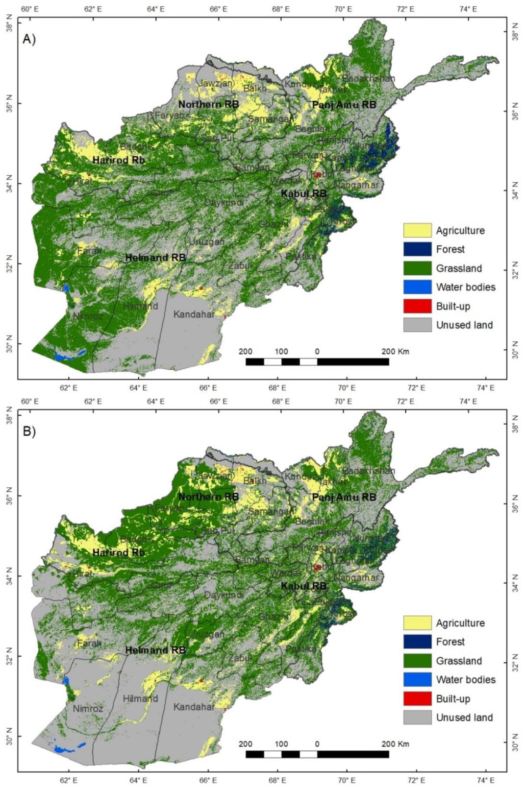
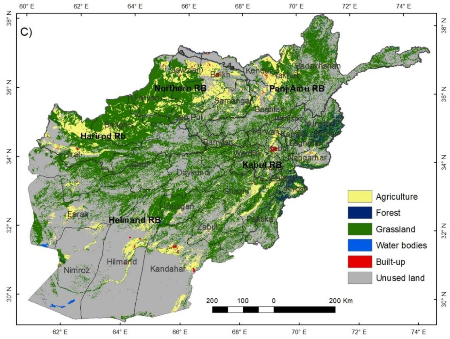
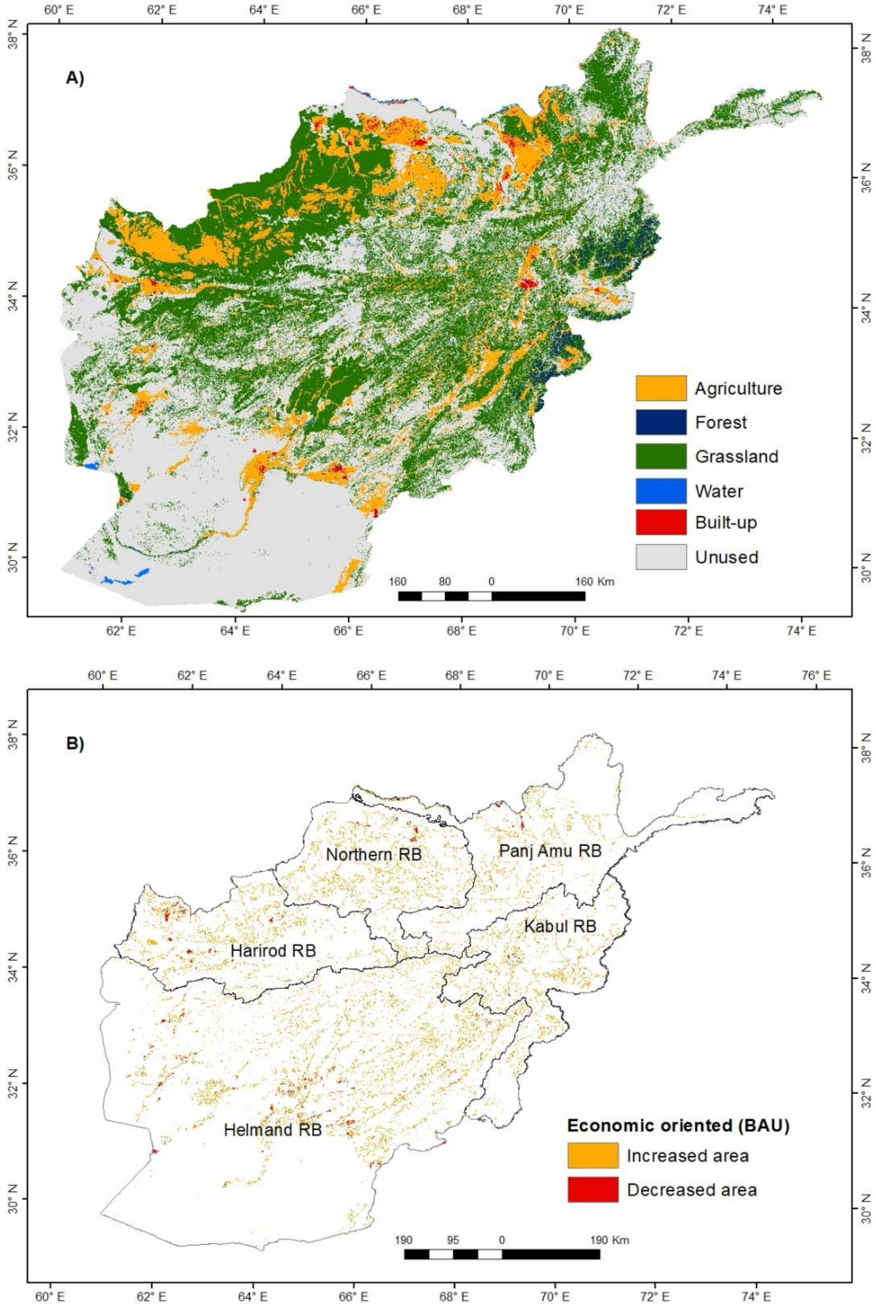
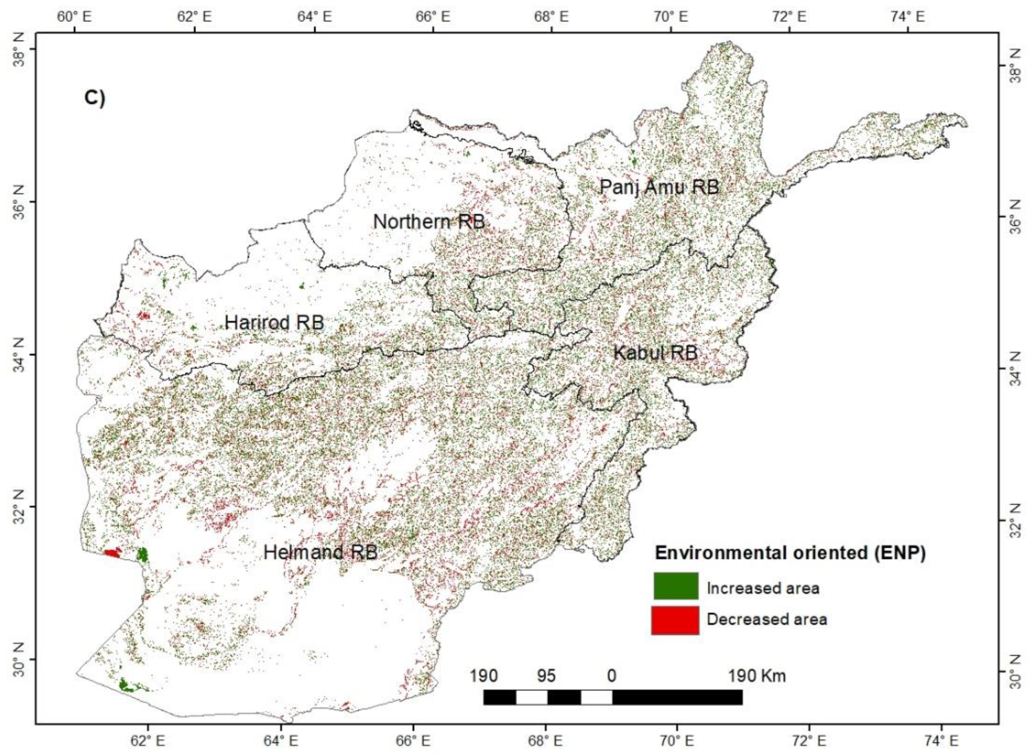
The spatial distribution of Afghanistan’s LULC in 2000, 2010 and 2020 is presented in Figure 4. A comparison of the six LULC types showed that unused land was the most dominant land type in Afghanistan, covering about 46% of the national total in 2000 (

Table 5. Magnitude of LULC change in Afghanistan.

Area in km2
Period	AG	FR	GR	WB	BT	UL	Total
2000	58,748	8776	276,230	2138	1035	298,908	645,835
2010	60,836	6927	248,382	2010	1076	326,604	645,835
2020	61,409	6967	247,875	2036	2262	325,286	645,835
% of total land
2000	9.1	1.36	42.8	0.33	0.16	46.25	100
2010	9.42	1.07	38.5	0.31	0.17	50.53	100
2020	9.51	1.08	38.4	0.32	0.35	50.34	100
% of change
2000–2010	3.6	−21.1	−10.1	−6.0	4.0	9.3	0
2010–2020	0.9	0.6	−0.2	1.3	110.2	−0.4	0
2000–2020	4.53	−20.61	−10.27	−4.75	118.50	8.83	0

). With proper investments, some proportion of these unproductive lands could potentially be used for economic or environmental purposes. From the remaining LULC area, about 44% was shared by environmental-oriented LULC types (i.e., grassland, forests, and water bodies), while less than 10% was shared by economic-oriented LULC types (agriculture and built-up). Grassland was the second most dominant land class, covering 42.8% of the total national area in 2000. Grassland is ecologically important and offers substantial provisioning and supporting ecosystem services in Afghanistan [100]. However, forestland and water bodies, that are considered to have highest ecosystem service values, together made up only about 2% of the area. Forest cover in Afghanistan is not only small, but tree density is also low [101].

As for economic-oriented LULC types, agricultural land occupied about 9.1% of the total national area in 2000. However, only about half of the agricultural land is used for cultivation; the remaining areas are left as fallows, mainly due to a lack of irrigation [3]. Investment in irrigation systems could, therefore, potentially make these lands suitable for cultivation, doubling the current agricultural production and boosting economic growth [102]. Built-up areas are the smallest LULC, covering less than 1% of the area. They are given a zero ecosystem service coefficient (as per Costanza, de Groot, Sutton, van der Ploeg, Anderson, Kubiszewski, Farber and Turner [22] study), even though their value for economic development is immense. The high concentration of built-up areas, however, can add to the pressure on natural lands and reduce ecosystem service supply.

The regional distribution of various LULC also shows significant variation. Most of the agricultural land is shared by Northern river (in the north) and Helmand river basins (in the south and southwest). Together, they make up about 60% of the agricultural land in Afghanistan. Most of the northern cultivated areas are a mix of irrigated and rainfed crops, while southern cultivated areas mostly comprise irrigation-based crops [42]. Forestland distribution, on other hand, is greatly skewed toward the Kabul river basin in the east of Afghanistan. This region possesses more than 80% of the total forests [43,44], mostly shared between the provinces of Paktia, Paktika, Kunar, and Nuristan. As for water bodies (comprise rivers, lakes and wetlands), more than 55% of them are in the Helmand river basin. The existence of these water bodies, coupled with irrigation infrastructure, has provided the basis for a comparatively higher concentration of irrigated agricultural land in this region [103,104]. Similarly, most of the built-up areas were distributed within Kabul and the Northern river basin; these areas also represent more than half of the built-up areas in Afghanistan.

A comparison of five river basins revealed that more than 50% of lands in Harirod and Kabul river basins are of environmental-oriented LULC types. The environmental-oriented land of Harirod is dominted by grassland, while in Kabul river basin is dominated by forests. As for the economic-oriented land, it is highly concentrated in the Northern river basin (23%), followed by Harirod (15%). This aligns with fact that the Northern river basin contained most of the agricultural and urban lands in 2000.

3.2. Magnititude of LULC Change

The overall magnitude change of LULC during the study period (i.e., 2000–2020) suggested that built-up land had increased at a maximal rate of 118% (

Table 6. Magnitude of LULC change in Afghanistan.

Area in km2
Period	AG	FR	GR	WB	BT	UL	Total
2000	58,748	8776	276,230	2138	1035	298,908	645,835
2010	60,836	6927	248,382	2010	1076	326,604	645,835
2020	61,409	6967	247,875	2036	2262	325,286	645,835
% of total land
2000	9.1	1.36	42.8	0.33	0.16	46.25	100
2010	9.42	1.07	38.5	0.31	0.17	50.53	100
2020	9.51	1.08	38.4	0.32	0.35	50.34	100
% of change
2000–2010	3.6	−21.1	−10.1	−6.0	4.0	9.3	0
2010–2020	0.9	0.6	−0.2	1.3	110.2	−0.4	0
2000–2020	4.53	−20.61	−10.27	−4.75	118.50	8.83	0

). This was followed by 8.8% increase of unused land and a 4.5% increase of agricultural land. On the other hand, forestland, grassland, and water lands decreased in size by 20.6%, 10.2%, and 4.7%, respectively. The most significant feature of LULC change during the study period was that the environmental development-oriented LULC types decreased in size, in contrast to economic development-oriented LULC types. The rapid increase of economic-oriented land was associated with massive socioeconomic growth. Since 2002, for instance, GDP and population have increased by at least 2.5 and 1.7 times, respectively [75,76]. On the other hand, rapid urbanization and population growth [105], unsustainable management [106], and challenging climatic conditions [107] are major causes of natural vegetation loss in Afghanistan.

A periodical breakdown of the study period shows that except for built-up land, the change rates of all LULC types during the first ten years were significantly higher than in the following ten years. The change rate of agricultural land, for instance, was by about four times more rapid from 2000 to 2010 (period I) than from 2010 to 2020 (period II). Similarly, the change rates of forestland, grassland, and water bodies were many fold faster in period I than in period II. Built-up land, however, grew 27 times more rapidly during the second period. In this period, the change rates of forest and water bodies shifted from decreasing to increasing. The decrease of grassland also slowed from 10.1% to 0.2%. Increased awareness of the importance of these landscapes could be a major reason of this shift in dynamics.

3.3. The Direction of LULC

The transition matrix (

Table 7. Direction of LULC change.

Transition Matrix of LULC Change (in Km2)
AG	FR	GL	WB	BL	UL
54452	80	2613	95	103	4066
16	4666	1457	8	0	820
2297	2963	174,294	232	24	68,063
181	29	276	1148	1	402
873	1	184	2	901	301
929	1037	97,406	653	6	225,255

Note 1: The non-diagonal figures in the table represent the changed area of each LULUC class during the period of 2000 to 2020, while the diagonal figures (in bold) represent the unchanged area of each class. The figures in the rows depict the area of other classes by ith class, while the columns show the area of ith class converted to another typology. Note 2: AG = Agricultural land, FR = forest area, GL = grassland, WB = water bodies, BL = built-up land and UL = unused land.

) shows the stability and change direction of six LULC types during the study period. From 2000 to 2020, agricultural and built-up land were the most stable LULC types. About 93% of agricultural land (i.e., 54,452 km² of 58,748 km²) and 87% of built-up land (i.e., 901 km² of 1035 km²) did not change. Meanwhile, the instability of forestland, water bodies, and grassland were noticeable, respectively remaining unchanged by only 53%, 54%, and 63%.

The directional changes show that the decrease in agricultural land was mostly a result of increases in grassland, unused land, and built-up areas. Notably, from the 4297 km² decrease in agricultural land, 2297 km² (53%), 929 km² (21%), and 873 km² (20%) were respectively converted to grassland, unused land, and built-up areas. During the same period, agricultural land also increased by about 6957 km², of which 4966 km² (58%) was formerly unused land and 2613 km² (38%) was formerly grassland. Similarly, the majority of the converted forestland became either grassland or unused land. From 4110 km² of forestland, 2963 km² became grassland and 1037 km² became unused land. Most of the changed grassland became unused land or forestland. Of the 101,936 km² of grassland, 97,406 km² changed to unused land and 2613 km² to agricultural land.

While water bodies and built-up land hold the smallest LULC proportions in Afghanistan, they are important indicators of environmental and economic development, respectively. From 2138 km² of water areas, about 990 km² was converted to other LULC types, mainly unused land (653 km² (66%)), grassland (232 km² (23%)), or croplands (95 km² (10%)). Productive agricultural land around residential areas was severely threatened by the expansion of built-up areas. This was evident by the fact that 77% of the built-up land expansion took place on agricultural land.

The severe instability of forests, grassland, and water bodies during the 20 year study period emphasizes the vulnerability of ecologically important LULC categories in Afghanistan. Likewise, the corresponding sprawl of economic development-oriented LULC into natural ecosystems implies increasing human expansion into natural ecosystems, as observed by others [105].

3.4. Ecosystem Services Pattern

Ecosystem services in Afghanistan largely comprise supporting services (SS) and provisioning services (PS). Together, these accounted for more than 80% of all ecosystem services in 2000 (

Table 8. Estimated values for various ecosystem functions in Afghanistan.

Service Type	Sub-Type	ESV (Billion $ ha−1 Year−1)			Change (%)
		2000	2010	2020	Period II	Period II
Provisioning	Total	49.68	46.74	46.8	−6.00	0.20
	Food production	46.81	43.97	44.03	−6.10	0.20
	Raw material	2.87	2.77	2.77	−3.50	0.00
Regulating	Total	21.41	25.5	22.97	19.20	−10.00
	Gas regulation	0.26	0.23	0.23	−11.60	0.00
	Climate regulation	5.32	4.93	4.95	−7.40	0.50
	Disturbance regulation	0.27	0.46	0.35	70.40	−24.00
	Water regulation	1.43	1.07	1.22	−25.20	14.10
	Water supply	4.38	4.23	4.27	−3.50	1.00
	Waste treatment	9.75	14.58	11.94	49.60	−18.20
Supporting	Total	82.85	76.55	76.12	−7.70	−0.60
	Erosion control	2.3	2.3	2.22	0.00	−3.50
	Soil formation	3.19	3.3	3.33	3.50	1.00
	Nutrient cycling	0.03	0.05	0.04	66.70	−20.00
	Pollination	1.12	1.02	1.02	−9.00	0.00
	Biological control	1.07	1.01	1	−5.70	−1.00
	Habitant/refugia	34.14	31.31	30.95	−8.30	−1.20
	Genetic resources	41	37.56	37.56	−8.40	0.00
Recreation & culture	Total	7.07	6.39	6.38	−9.70	−0.20
	Recreation	2.42	2.18	2.19	−10.00	0.50
	Cultural	4.64	4.21	4.18	−9.30	−0.80
	Grand Total	161	155.19	152.27	−3.70	−1.90

). Cultural services (CS), on the other hand, made the smallest contribution, i.e., only 4.3%. The overall value of ecosystem services during the 20 year study period was reduced by 5.4% (8.73 billion USD). This decline was mainly driven by a 65% decrease of RS and a 27% decrease of PS services. Positively, regulating services (RS) during the study period increased by nearly 7.2% (1.6 billion USD). A comparison of the two periods showed that the decline of ESV during period I was by nearly two times greater than that in the later period. A total ESV reduction of 5.8 billion USD and 2.9 billion USD during periods I and II was estimated, respectively. The higher decline in ESV during first period was attributed to a rapid decrease in environmental-oriented LULC change.

As for the ESV changes of various groups during period I, all groups apart from RS showed decreasing trends. Although CS value was found to have the highest annual decline rate of 1%, the largest contributions to the overall ESV decrease also came from RS (64%) and PS (28%). Rapid annual rates of decline of SS (about 0.8%) and PS (about 0.6%) were also noticeable during this period. In contrast, the value of RS was found to have the highest change rate, i.e., about a 2% annual increase. During the later period, however, this positive trend changed drastically, becoming the highest declining trend. The other noticeable feature of period II was that the PS value changed to positive while the values of the remaining groups retained their negative trends. Importantly, the annual decreasing trend of SS and CS were significantly slowed.

Overall, the negative change in ESV was significantly slower during period II compared to period I. This could be associated with increased awareness of the importance of the ecosystem, which resulted in enhanced management of ecosystems. With the involvement of the USA and allied nations during the initial years of period I, a new governmental setup with low capacity was formed that inefficiently used most of the received funding for economic development without consideration of the environmental consequences. However, this scenario gradually changed and investments were later used more effectively, resulting in a slowing of the negative impact on LULC and ESV changes in Afghanistan.

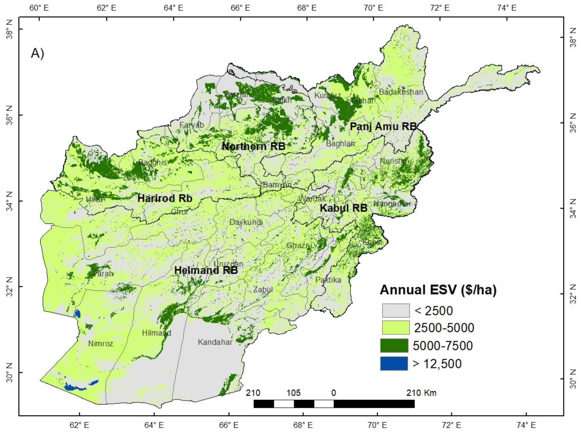
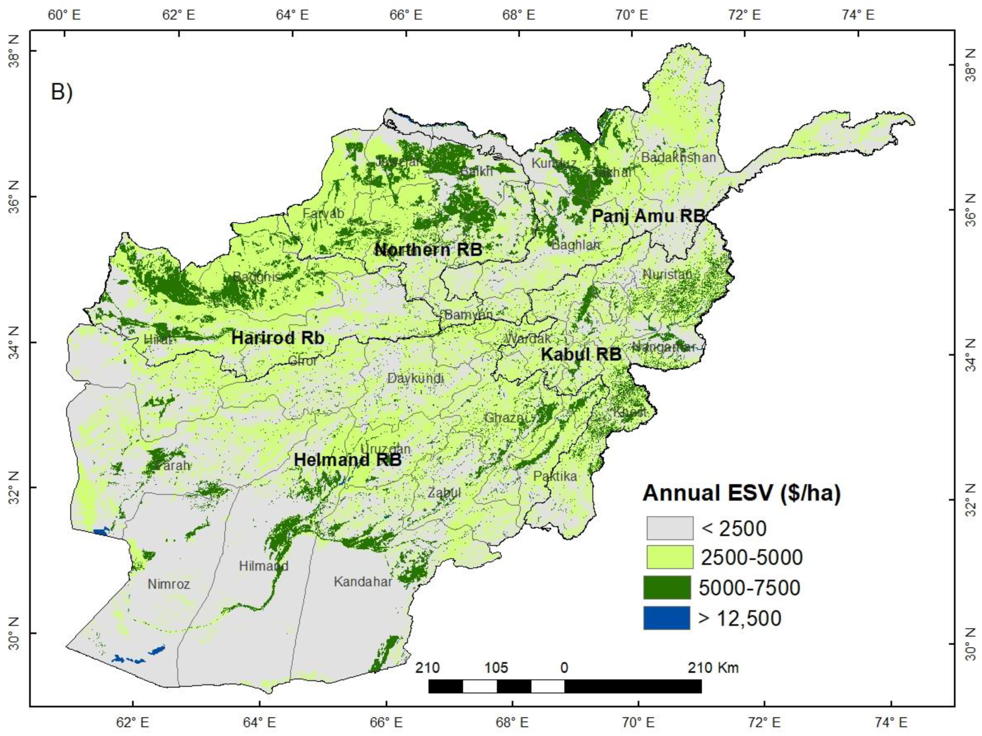
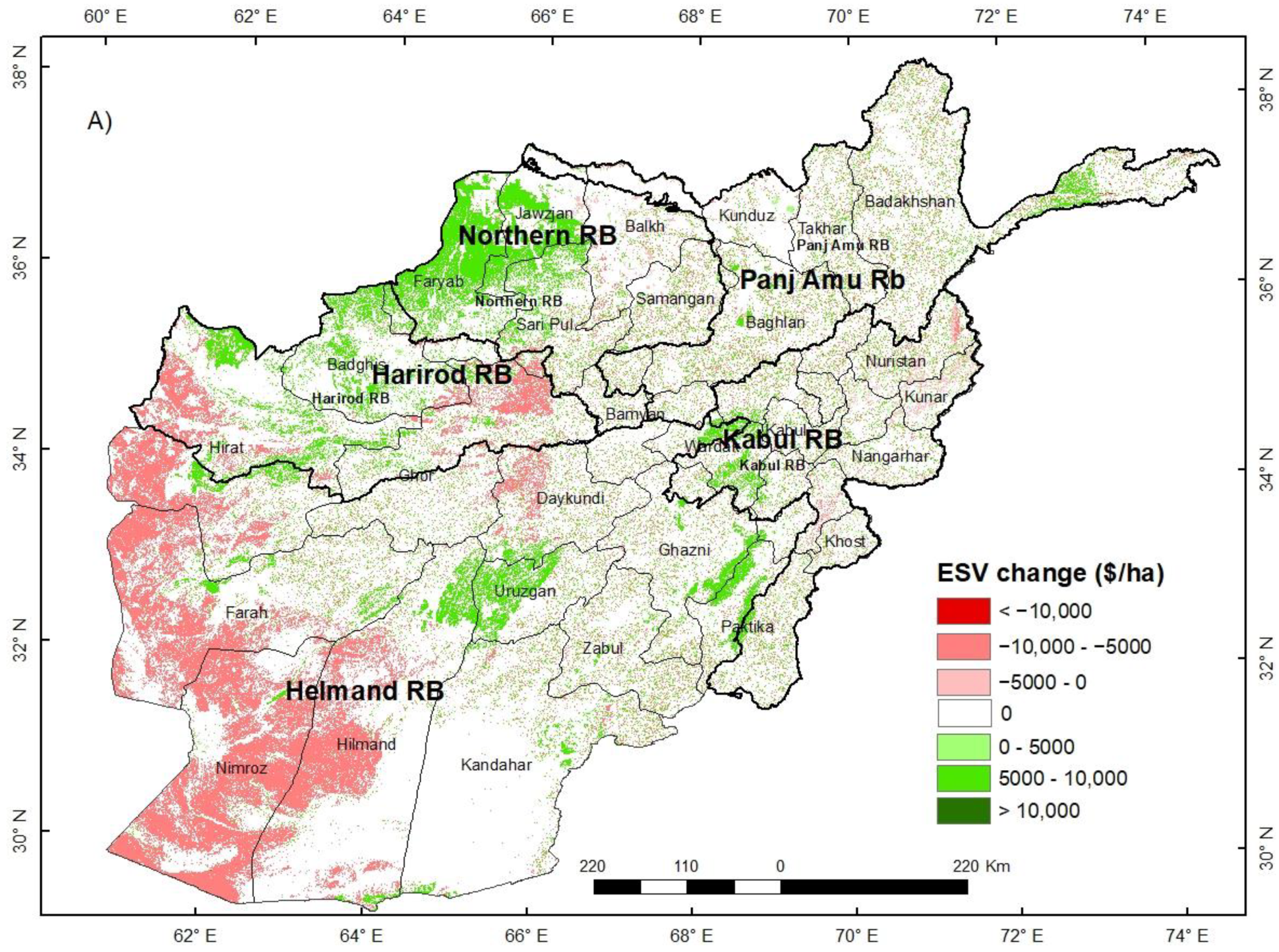
From the perspective of the spatial distribution of ESV, the north and northwest regions (stretching from the Harirod basin to the Amu basins) contained many of the hotspots for ESV (Figure 5). The annual per ha ecosystem service value in these hotspots reached up to 7500 USD. On the other hand, the south and southwest regions contained large patches of land with near to zero ESV. Nonetheless, a few patches with high ESV were located in this region. The annual per ha ESV of these hotspots reached more than 12,500 USD. Furthermore, this region also showed the most noticeable spatial changes of ESV from 2000 to 2020. During these periods, large areas in this region were from moderate (<5000 USD ha⁻¹ yr⁻¹) to small ESV (<250 USD ha⁻¹ yr⁻¹).

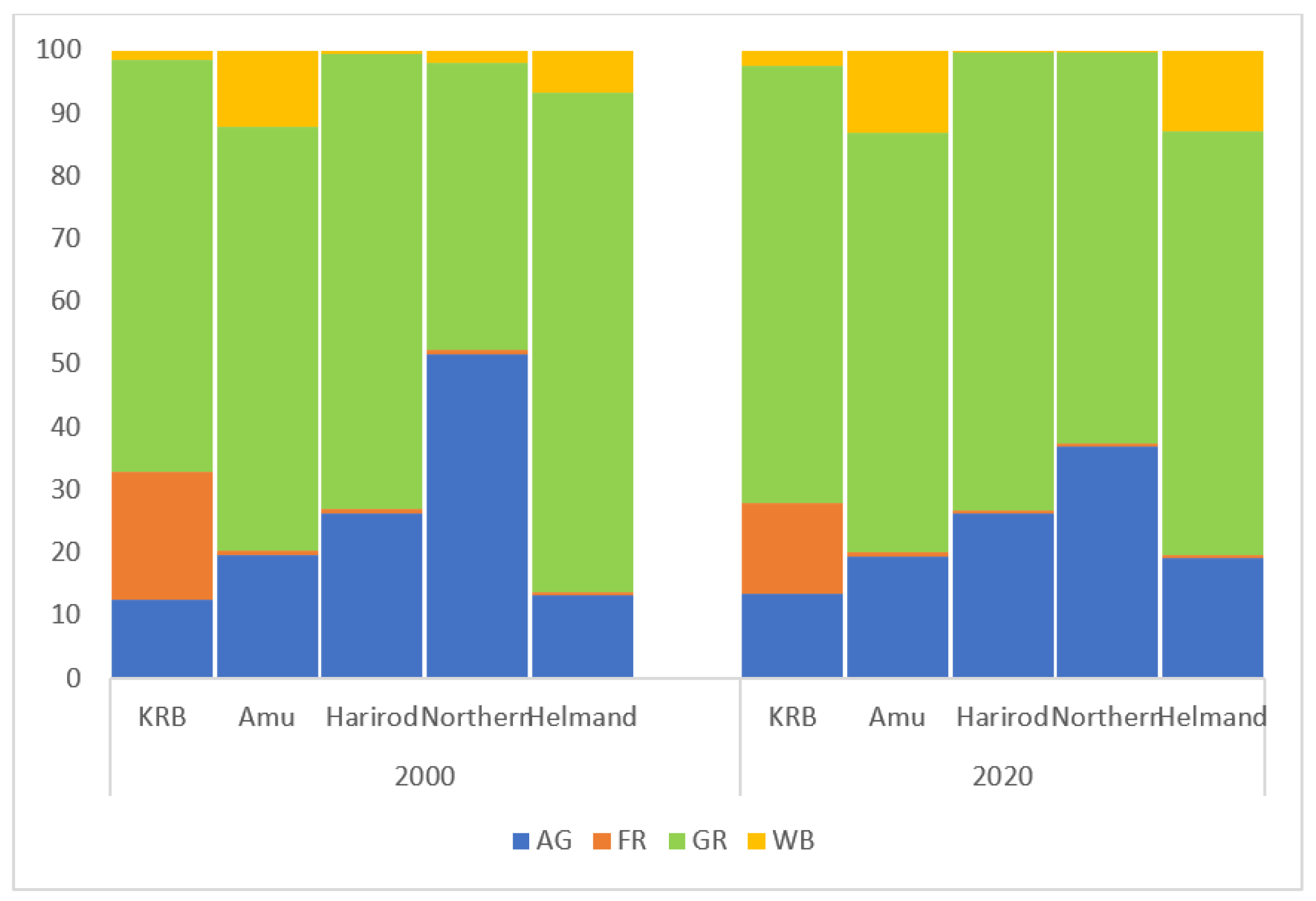
Overall, grassland was the second biggest LULC type in Afghanistan, accounting for more than 70% of the total ESV in 2000 (Figure 6). The highest contribution was grassland, followed by agricultural land, with more than 20%, and water bodies, with more than 5%. The percentage of forest cover reached nearly 2.5%. A comparison of the river basins also revealed that (except for Northern river basin) the contributions of grassland ecosystem services to total ESV were the highest across all river basins in 2000. Agricultural land, as the second greatest contributor, provided the highest share in the Northern river basin. The share of agricultural land in other regions was also noticeable. Water ecosystem services were most significant in the Amu and Helmand river basin regions. More than 80% of the forest ecosystem in Afghanistan was concentrated toward the eastern region, i.e., the Kabul river basin. However, these forest services were considerably reduced during the 2000–2020 period. The decrease of agricultural land in the Northern river basin was also notable during that time. On the positive side, the contributions of water ecosystems in the Amu and Helmand river basins increased. This may have resulted from the substantial investments in water storage capacity enhancement during the study period.

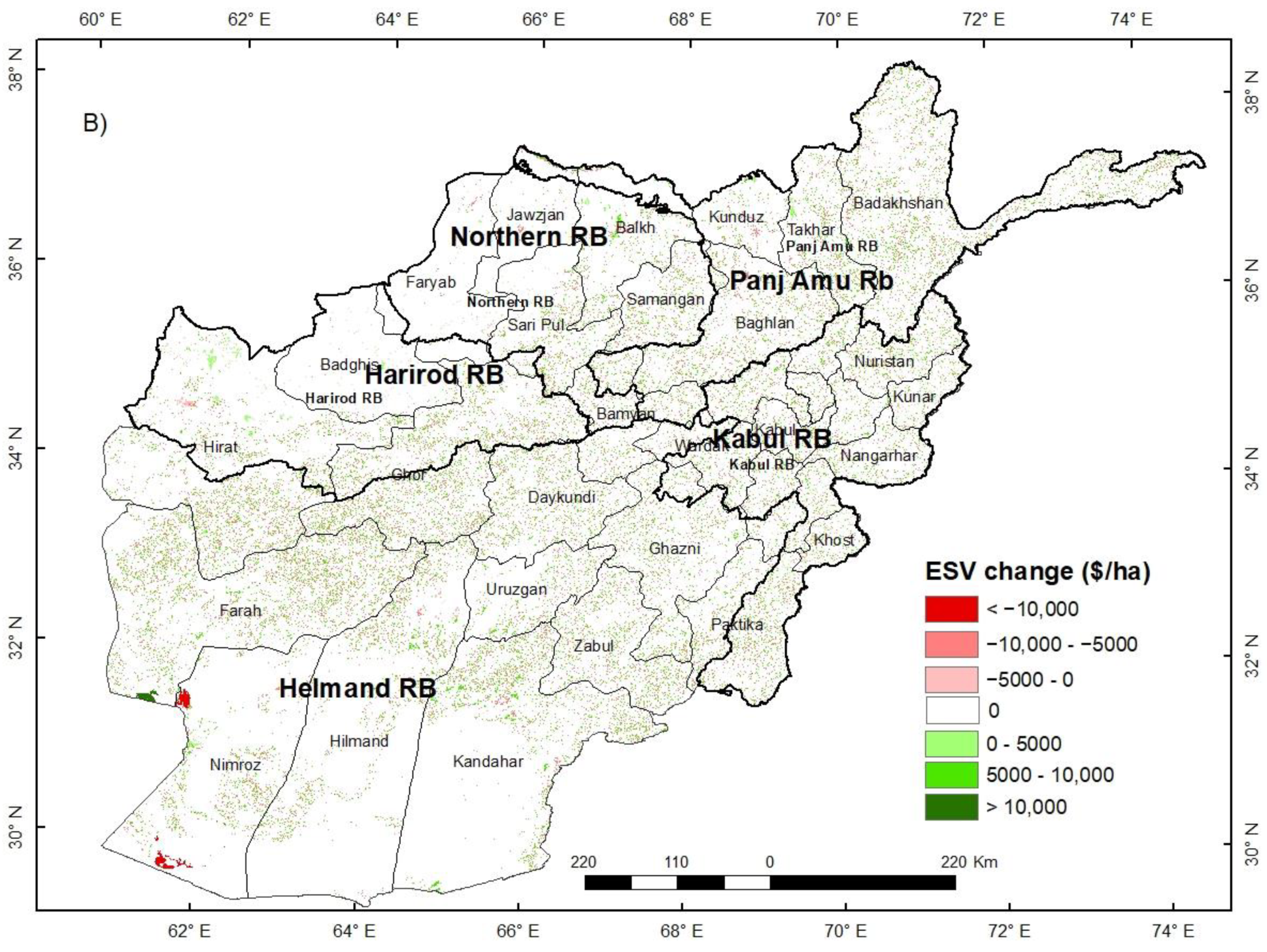
The spatial distribution of ESV change during periods I and II is shown in Figure 7. The figure clearly shows that ESV changes throughout the country were more prominent in period I as compared to period II.

3.5. LULC and ESV Simulations

3.5.1. LULC Simulation Results

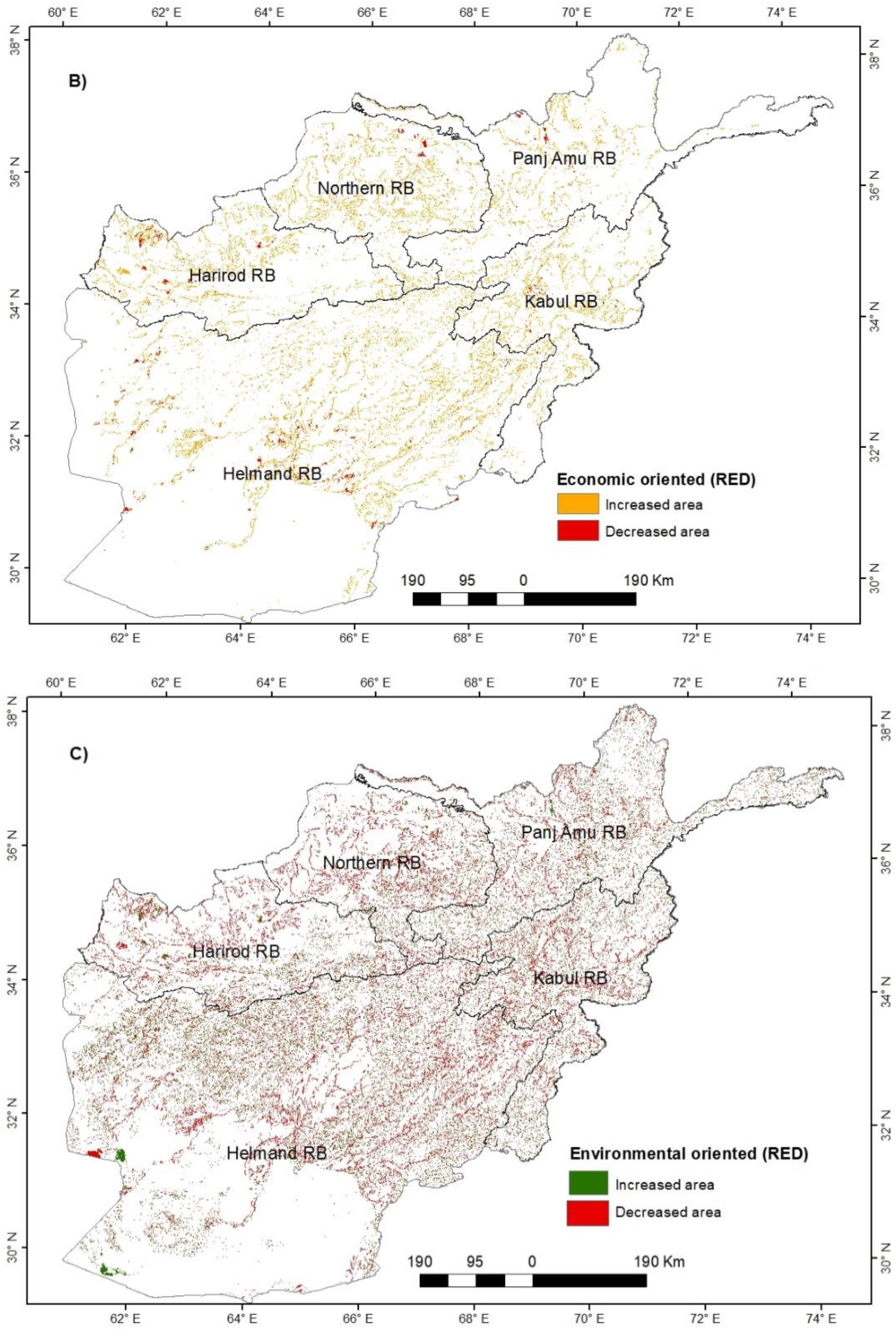
The spatial distribution of the simulated LULC under the business-as-usual, rapid economic development and environmental protection scenarios are presented in Figure 8, Figure 9 and Figure 10, respectively. The simulation under the BAU scenario predicted subtle changes of economic-oriented LULC classes, as compared to environmental-oriented LULC types (Figure 8B). Furthermore, a spatial increase of economic-oriented LULC types was predicted. Importantly, the spatial distribution of economic-oriented LULC was predicted to occur in scattered pattern across the entire country. On the other hand, environmental-oriented LULC types (Figure 8C) were predicted to undergo significant changes. However, the spatial patterns of the predicted increased and decreased areas of environmental-oriented LULC types did not show any significant difference. Additionally, the predicted changes were concentrated in the eastern and central regions, particularly in the Kabul river basin.

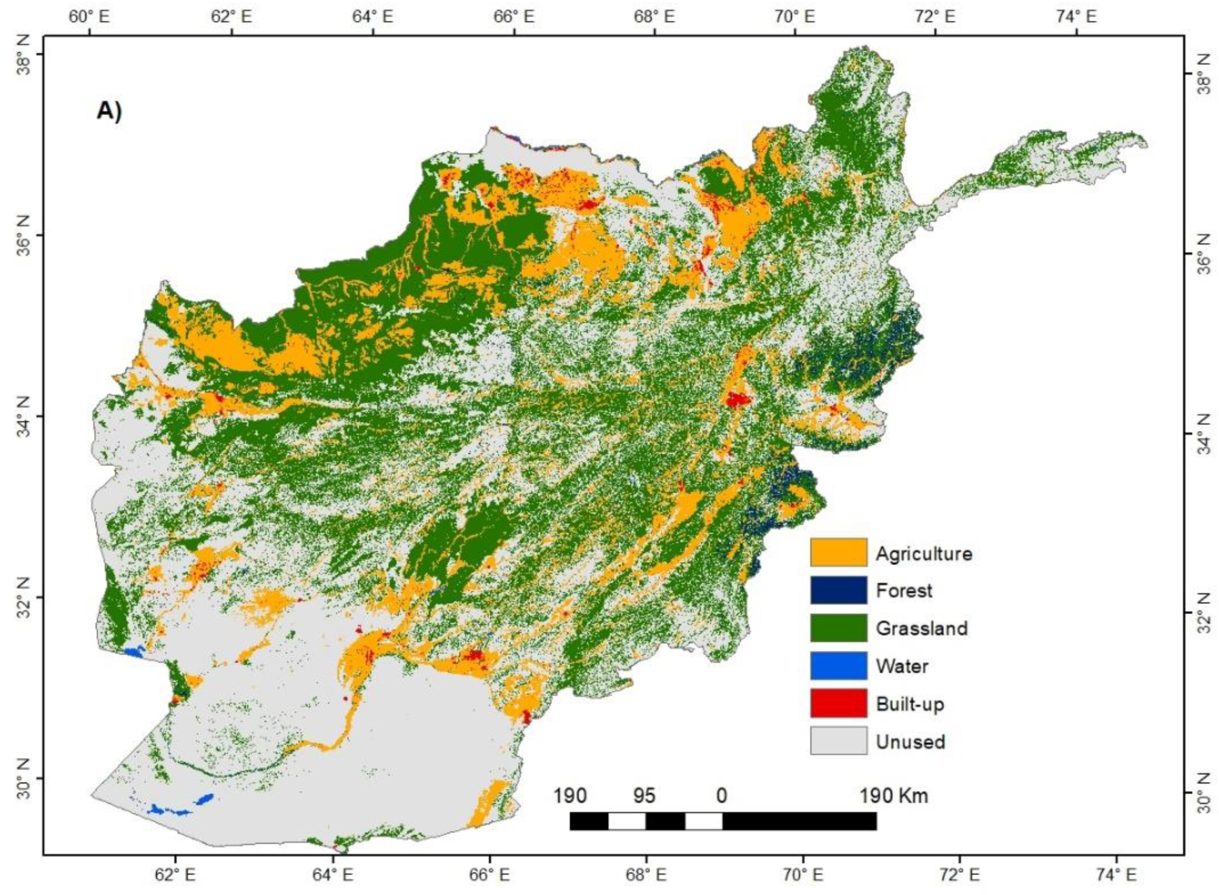
The RED scenario represented a situation where rapid economic development becomes a central focus of governmental development planning. The spatial simulation LULC under that scenario predicted significant changes in economic-oriented LULC types, as compared to other two scenarios (Figure 9). The increase of economic-oriented LULC classes was also predicted to be significantly higher than their decrease. Similar to the BAU scenario, the overall distribution of increased economic-oriented LULC types was predicted to be scattered over the study area (Figure 9B), with a slightly higher concentration being predicted in the eastern region. The eastern region is considered to be a socioeconomic development hub, where major economic cities such as Kabul, Jalalabad, and Khost are located. The north and northwest regions were also predicted to show a considerable increase in economic-oriented areas. The main economic development of these regions would be driven by agricultural land development, as they account for a high proportion of the total agricultural area in Afghanistan [42]. The predicted spatial pattern of environmental-oriented lands followed a more or less similar pattern to that of the BAU scenario (Figure 9C). However, understandably, the decrease of environmental development-focused land was higher here. This implies that if development policies are focused only on rapid economic development, environmental degradation could occur more rapidly. Similar to BAU, most of the predicted changes in environmental-oriented lands under the RED scenario were concentrated in the eastern and central regions.

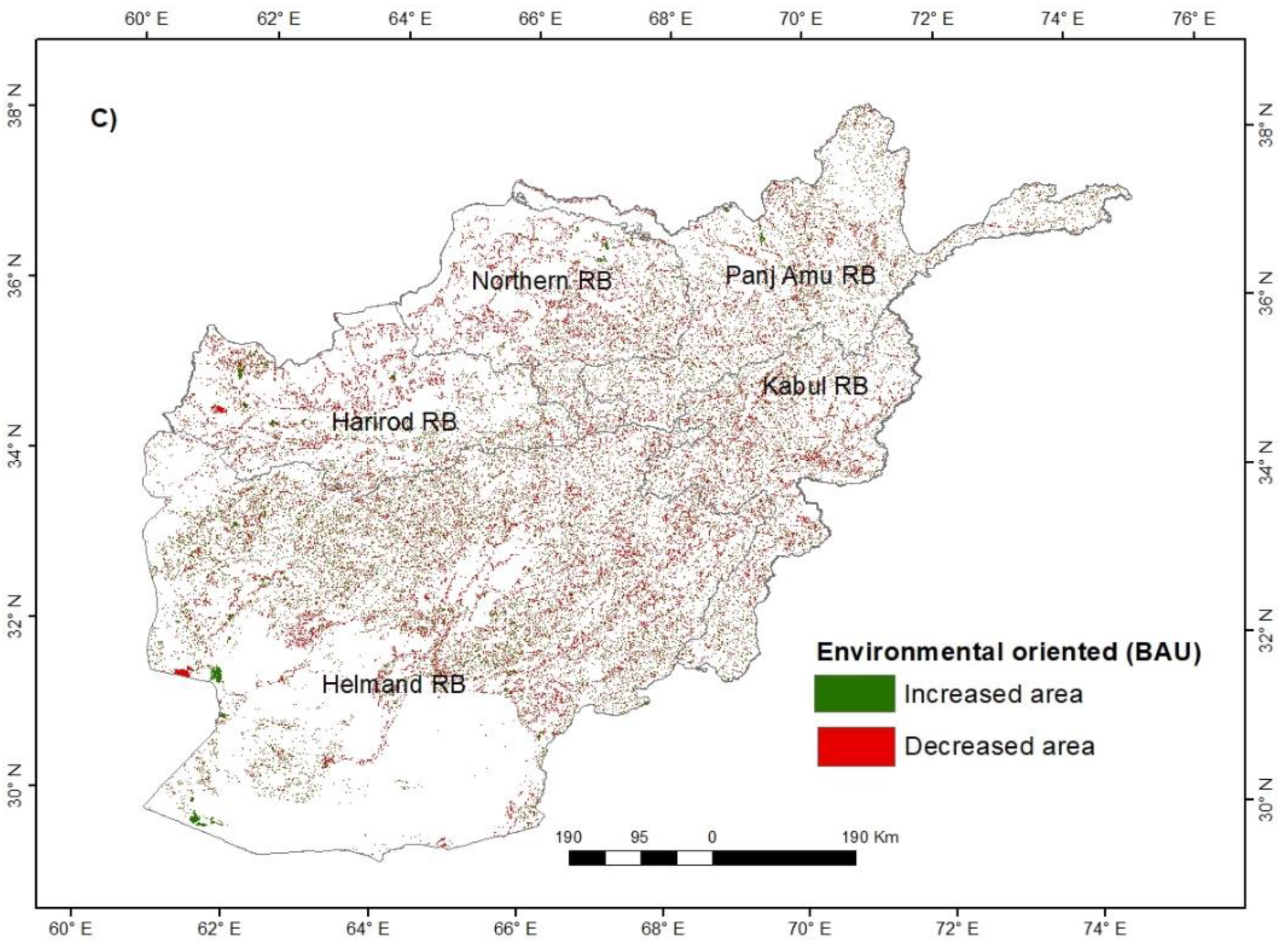
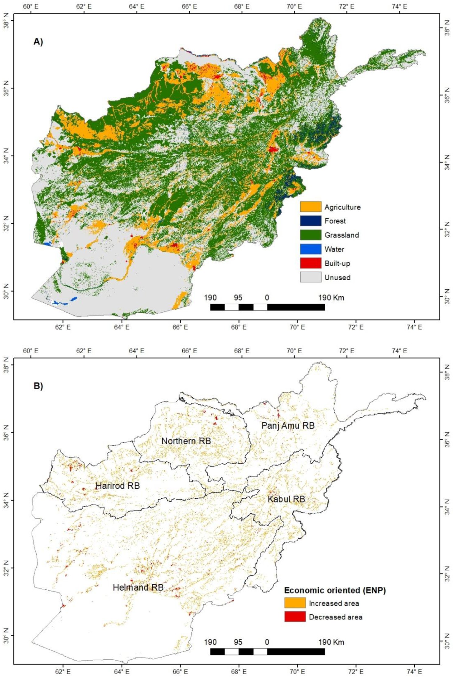
The ENP scenario represents a situation where environmental protection becomes the main focus of development policies. The spatial distribution of LULC under that scenario predicted significant change in economic-oriented LULC types, similar to the BAU scenario (Figure 10B). However, the predicted decrease in areas of economic-oriented land was noticeably higher than in the BAU scenario. Most importantly, environmental-oriented LULC types were expected to undergo significant growth (Figure 10C). As a result of strict environmental protection measures, this scenario would likely lead to the restoration of large areas degraded grasslands, forest, and water bodies. For instance, the conversion of vast areas of grasslands to economic-oriented classes in the north and northwest was predicted to significantly slow, in contrast to the expected outcomes under the other two scenarios.

The predicted magnitude changes of six LULC types by 2030 are presented in

Table 9. LULC dynamics in actual and predicted scenarios.

Scenario	Year	AG	FR	GR	WB	BL	UL
Actual	2020	61,409	6967	247,875	2036	2262	325,286
BAU	2030	61,988	6934	247,438	2070	3413	323,992
	Change	0.93	−0.48	−0.18	1.64	33.72	−0.40
RED	2030	62,288	6624	246,838	2020	3863	324,202
	Change	1.4	−5.2	−0.4	−0.8	41.4	−0.3
ENP	2030	61,915	7796	247,956	2202	3264	322,702
	Change	0.82	10.63	0.03	7.54	30.70	−0.80

. The BAU scenario predicted that forest, grassland, and unused land will likely decrease by 0.48%, 0.18% and 0.40%, respectively, and be converted to typologies. Their decrease will add to the size of remaining LULC types. Under this scenario, agricultural land, water bodies, and built-up areas are likely to grow by 0.93%, 1.64%, and 33.72%, respectively. The RED scenario predicted substantial growth of agricultural and built-up lands, i.e., by 1.4% and 41.4%, respectively. However, due to rapid expansion of economic-oriented lands, forests, grassland, and water bodies are likely to be affected, leading to reductions of 5.2%, 0.4% and 0.8%, respectively. On the other hand, the ENP scenario will increase the protection of these ecologically important lands. Under that scenario, the expansion of agricultural land and built-up land will slow, which will reduce the vulnerability of forest, grassland, and water areas, and forests and water areas will increase by 10.63% and 7.54%, respectively; grassland will also increase by 0.03%. From the prospective of ecosystem service protection, this scenario is the best options for policy makers.

3.5.2. Predicted ESV

The predicted values of various ecosystem services under all of the studied scenarios are presented in the

Table 10. Simulated scenarios of total ESV of Afghanistan.

Service Type	Sub-Type	Actual (2020)	BAU (2030)		RED (2030)		ENP (2030)
		ESV	$\mathbf{ESV} ({10}^{-9}\$)$	Change (%)	$\mathbf{ESV} ({10}^{-9}\$)$	Change (%)	$\mathbf{ESV} ({10}^{-9}\$)$	Change (%)
Provisioning	Total	46.8	46.88	0.16	46.87	0.15	46.91	0.25
	Food production	44.03	44.1	0.16	44.09	0.14	44.13	0.22
	Raw material	2.77	2.77	0.18	2.78	0.2	2.79	0.59
Regulating	Total	22.97	21.82	−5.27	21.73	−5.42	23.52	2.38
	Gas regulation	0.23	0.23	0.43	0.23	0.04	0.23	0.94
	Climate regulation	4.95	4.96	0.28	4.91	−0.76	5.14	3.88
	Disturbance regulation	0.35	0.3	−16.73	0.3	−14.9	0.36	3.86
	Water regulation	1.22	1.32	7.5	1.28	4.99	1.35	10.38
	Water supply	4.27	4.31	0.93	4.31	0.91	4.32	1.25
	Waste treatment	11.94	10.7	−11.63	10.7	−10.43	12.11	1.41
Supporting	Total	76.12	75.91	−0.28	75.75	−0.49	76.31	0.25
	Erosion control	2.22	2.18	−1.87	2.17	−2.27	2.25	1.47
	Soil formation	3.33	3.36	0.8	3.37	1.27	3.35	0.73
	Nutrient cycling	0.04	0.03	−17.71	0.03	−15.27	0.04	3.79
	Pollination	1.02	1.02	0.31	1.02	0.08	1.03	0.59
	Biological control	1	1	−0.4	0.99	−0.52	1	0.09
	Habitant/refugia	30.95	30.75	−0.64	30.68	−0.87	30.93	−0.07
	Genetic resources	37.56	37.56	0	37.47	−0.23	37.7	0.38
Recreation & culture	Total	6.38	6.37	−0.14	6.32	−0.86	6.49	1.65
	Recreation	2.19	2.2	0.55	2.17	−1.09	2.31	5.32
	Cultural	4.18	4.17	−0.27	4.16	−0.51	4.18	−0.03
Total ESV		152.27	150.97	−5.53	150.67	−6.62	153.22	4.53

. Overall, more than 80% of the predicted ESV under all three scenarios are composed of supporting services (SS) and provisioning services (PS), while regulating (RS) and cultural services (CS) share less than 20% of the total ESV. This trend is aligned with the ESV estimated using actual LULC. By 2030, ESV under the RED and BAU scenarios were predicted to undergo further declines of 6.6% and 5.5%, respectively. Under these scenarios, all four groups of ecosystem services i.e., PS, SS, CS and RS, will decrease. The highest predicted decline of ESV under the RED scenario would mainly be driven by the 6.4% decrease of environmental-oriented LULC types.

On the other hand, the ESV with ENP scenarios will increase by about 4.5% and will add another 1 billion USD to the ESV in 2020. This scenario is likely to boost the value of all four types of ecosystem services. The highest value addition under this scenario was predicted for regulating services, i.e., a 2.38% increase in 10 years. The second highest increase was predicted for recreational and cultural services, with a 1.65% increase. Although this scenario is the most desirable from the prospective of ecosystem management, its implementation depends heavily on the implementation of rational environmental protection measures and efficient management efforts.

4. Discussion

4.1. Impact of LULC Change on Ecosystem Services in Afghanistan

In Afghanistan, LULC management is important, as people’s livelihoods are heavily dependent on local landscape services. Grassland, agricultural land, forest, water bodies, and built-up land are important LULC classes in Afghanistan that are used for economic and environmental purposes. Depending upon the regional conditions, the distribution of economic- and environmental-oriented LULC types varies significantly around the country. The 20 year LULC change analysis showed that the economic-oriented LULC types such as agricultural and built-up land had increased by 4.5% and 118%, respectively. This increase in economic-oriented land was synchronized with the rapid growth of GDP and population [60]. However, in contrast to economic-oriented LULC types, the size of environmental-oriented LULC types such as forest, grassland, and water bodies were reduced by 20.6%, 10.2%, and 4.2%, respectively. Furthermore, severe instability in environmental-oriented LULC classes during the study period were noticed, which emphasizes the vulnerability of these LULC classes in Afghanistan. Various studies have reported rapid urbanization [105], poor management [106], and worsening climatic conditions [107] as some of the major underlining reasons of environmental-oriented land cover loss.

However, the study period breakdown analysis revealed improved conditions for environmental-oriented LULC classes during the second period. From 2010 to 2020 (period II), the negative change trends of forest and water bodies were shifted to positive, and the decreasing rate of grassland slowed from 10.1% to 0.2%. Increased awareness among decision makers of the importance of environmental-oriented LULC types could be a major driver of this shift. It is also noticeable that due to massive reductions of foreign funding during period II, economic development-related investment was significantly reduced. This scenario possibly minimized the pressure on natural ecosystems, leading to improved ecological conditions.

By using the Costanza et al. (2014) coefficients coupled with the study area NDVI and GDP information and the estimated size of the six LULC biomes, we determined that the total ESV in Afghanistan was reduced by 5.4% (8.73 billion USD) from 2000 to 2020. This negative change was mainly attributed to massive grassland and forest land changes, especially during first ten years. Grassland ecosystems alone account for more than 70% of the total ESV in Afghanistan, followed by agricultural land at 20%. The second period of the study expectedly revealed a much slower decreasing trend of ESV. This trend was aligned with the improved conditions of environmental-oriented LULC classes during these years. The spatial distribution of ESV across the regions of Afghanistan were also proportional to the composition of LULC classes.

From the prospective ecosystem management, the simulation results of LULC and ESV revealed a worse situation with the RED scenario. By 2030, ESV under this scenario will further decrease by about 6.6%, followed by the BAU scenario, with a 5.5% decrease. This is aligned with fact that rapid economic development accelerates the conversion of environmental-oriented LULC types to the highest rate (6.4%), which will result in a further decline of ecosystem service supplies. This situation is particularly likely when the implementation of environmental protection plans is subject to water, land, and money constraints [46,61,65,66]. Focusing on only rapid economic development will further divert these resources from environmental development projects to industrial and agricultural development, which may result in the loss of ecosystem services.

On the other hand, the ENP scenario was predicted to yield the highest growth of ESV by 2030. ESV in this scenario will increase by 4.5% and will add another 1 billion USD in 2020. The values of all four types of ecosystem services are expected to grow under this scenario. As such, this scenario is the most desirable one as far as ecosystem services sustainability is considered. However, the successful achievement of this scenario largely depends on meeting reforestation goals, i.e., 60,000 ha each five years, and ending the current degradation of rangelands and water areas [53]. Therefore, rationalized environmental protection measures and efficient management efforts are urgently needed. Considering the low capacity of the current government, the support of international organizations, especially those providing funds for the restoration and protection of natural land in Afghanistan, will be of major significance.

The overall results of our study reveal that the expansion of economic-oriented land such agricultural and built-up lands has led to decreased of natural land and ESV. This result is aligned with the findings of other studies that used similar ESV assessment methods in other regions of the world [12,108,109,110].

4.2. Limitation of the Study

Some methodological limitations should be noted in the applied benefit transfer method. The major one comes from the assumption of ecosystem service value homogeneity within the entire range of LULC classes, which allows the use of average unit values estimated in another place for specific goods to the current study area [32,111]. The services may have higher value in some areas than in the original study area [24,112]. Furthermore, this method is also assumed to be valid only after empirical links between ecosystem characteristics and final services have been established [113]. In this study, we tried to minimize the effect of this limitation by incorporating specific information from some study areas, like NDVI and GDP, into the adopted coefficients. Despite these shortcomings, the BTM approach may be the best option for researchers to cost-effectively and rapidly assess multiple ecosystem services at large geographical scales [113]. The other limitation of this study comes from data scarcity. Afghanistan is a data-scarce region; much of the required data is either not available or of low quality. For instance, the incorporation of the angel coefficient [43] to the adopted coefficients would have further improved our results. However, this was avoided due to the unavailability of this data in Afghanistan.

5. Conclusions and Recommendations

A high level of dependency on LULC-induced services has increased the risk of ecosystem service loss in Afghanistan. This dynamic underlines the need of economic valuations of ecosystem services. This study fills this research gap and provides a much-needed national assessment of the impact of LULC changes on ESV in Afghanistan from 2000 to 2020. Furthermore, it provides a future prospective of various ESV scenarios. The results of this study reveal significant LULC changes in Afghanistan during 2000 to 2020. The overall LULC change analysis revealed that while economic-oriented LULC types increased, environmental development-oriented LULC types such as forest cover, grassland, and water bodies decreased by 20.6%, 10.2%, and 4.7%, respectively. The directional changes of these LULC types also indicated their instability and vulnerability, compared to agriculture and built-up lands. The ESV analysis showed that 80% of the ecosystem services in Afghanistan serve to support and provide services. During the entire study period, the total ESV declined from 161 billion USD in 2000 to 152.27 billion USD in 2020, which is a nearly 5% reduction. The highest decrease of value was estimated in cultural services, followed by supporting and regulating services. However, the rate of decrease was considerably slower during the last 10 years (3.7%) compared to the initial 10 years (1.9%). This could have been due to increased awareness among decision makers of the importance of ecosystem services.

The simulation results revealed that built-up and agricultural land will grow the least under the ENP scenario, i.e., by 0.8 and 30.7%, respectively, while, they will grow faster under the RED scenario, i.e., by 1.4% and 41.4%, respectively. However, the rapid economic development of the RED scenario will accelerate the reduction of forest, grassland and water areas by 5.2%, 0.4% and 0.8%, respectively.

On a more positive note, the expansion of natural lands such as forests, grassland, and water areas were predicted to occur more rapidly under the ENP scenario. Under ENP, the expansion of agricultural and built-up land will slow down, reducing the pressure on forest, grassland, and water areas. Under this scenario, forest and water areas will increase by 10.6% and 7.5%, respectively. The overall predicted ESV also largely consists of supporting and provisioning services. The overall ESV under RED and BAU is likely to further decline from 152.27 to 150.6 and 150.9 billion USD by 2030. The decline of ESV in the RED scenario was the highest; this is a result of the rapid decrease of environmental-oriented LULC types. On the other hand, ESV under ENP will likely increase from 152.27 to 153.22 billion USD. This situation could occur if 60,000 ha of reforestation every 5 years is maintained and degraded rangelands and water areas are restored. However, this would require substantial resources and better execution.

The current decreasing ESV trend suggests the need for a more balanced approach of economic and environmental development. This is required for the comprehensive development of nations. Some quick actions, such as providing alternative fuel sources, will reduce the pressure on forests in the short term. Currently, forest resources are widely used for household energy. Also, the support of international donors may play a significant role in the implementation of environmental development programs. Government and non-government partners need to work with local communities to increase the management capacities of the latter. The rapidly growing population is a major challenge for ecosystem management. It is perhaps time for Afghanistan to take steps regarding population control, obviously while respecting the nuances of local culture. Lastly, as water management remains the most crucial factor for both economic and environmental development, suitable measures need to be taken to optimize water utilization, both through constructing water storage facilities and improving water use efficiency.

References

1. Skewes, T.; Hunter, C.; Butler, J.; Lyne, V.; Suadnya, W.; Wise, R. The Asset Drivers, Well-being Interaction Matrix (ADWIM): A participatory tool for estimating future impacts on ecosystem services and livelihoods. Clim. Risk Manag. 2016, 12, 69–82. [Google Scholar] [CrossRef] [Green Version]
2. Butler, J.; Suadnya, W.; Puspadi, K.; Sutaryono, Y.; Wise, R.; Skewes, T.; Kirono, D.; Bohensky, E.; Handayani, T.; Habibi, P. Framing the application of adaptation pathways for rural livelihoods and global change in eastern Indonesian islands. Glob. Environ. Chang. 2014, 28, 368–382. [Google Scholar] [CrossRef]
3. Zhan, J. Impacts of Land-use Change on Ecosystem Services; Springer: Berlin/Heidelberg, Germany, 2015. [Google Scholar]
4. Costanza, R.; d’Arge, R.; De Groot, R.; Farber, S.; Grasso, M.; Hannon, B.; Limburg, K.; Naeem, S.; O’neill, R.V.; Paruelo, J. The value of the world’s ecosystem services and natural capital. Nature 1997, 387, 253–260. [Google Scholar] [CrossRef]
5. Millennium Ecosystem Assessment. Ecosystems and Human Well-Being; Island Press: Washington, DC, USA, 2005; Volume 5. [Google Scholar]
6. de Groot, R.S.; Alkemade, R.; Braat, L.; Hein, L.; Willemen, L. Challenges in integrating the concept of ecosystem services and values in landscape planning, management and decision making. Ecol. Complex. 2010, 7, 260–272. [Google Scholar] [CrossRef]
7. Alcamo, J.; Van Vuuren, D.; Cramer, W.; Alder, J.; Bennett, E.; Carpenter, S.; Christensen, V.; Foley, J.; Maerker, M.; Masui, T. Changes in ecosystem services and their drivers across the scenarios. Ecosyst. Hum. Well-Being 2005, 2, 297–373. [Google Scholar]
8. Quintas-Soriano, C.; Castro, A.J.; Castro, H.; García-Llorente, M. Impacts of land use change on ecosystem services and implications for human well-being in Spanish drylands. Land Use Policy 2016, 54, 534–548. [Google Scholar] [CrossRef]
9. Deng, X.; Li, Z.; Huang, J.; Shi, Q.; Li, Y.; Zhang, R.; Huang, J. Reviews on impact assessments of land-use change on key ecosystem services. In Impacts of Land-Use Change on Ecosystem Services; Springer: Berlin/Heidelberg, Germany, 2015; pp. 1–35. [Google Scholar]
10. Ellis, E.; Pontius, R. Land-use and land-cover change. Encycl. Earth 2007, 1, 1–4. [Google Scholar]
11. Lambin, E.F.; Meyfroidt, P. Global land use change, economic globalization, and the looming land scarcity. Proc. Natl. Acad. Sci. USA 2011, 108, 3465–3472. [Google Scholar] [CrossRef] [Green Version]
12. Chen, J.; Sun, B.-M.; Chen, D.; Wu, X.; Guo, L.-Z.; Wang, G. Land use changes and their effects on the value of ecosystem services in the small Sanjiang plain in China. Sci. World J. 2014, 2014, 752846. [Google Scholar] [CrossRef] [Green Version]
13. Robertson, G.P.; Swinton, S.M. Reconciling agricultural productivity and environmental integrity: À grand challenge for agriculture. Front. Ecol. Environ. 2005, 3, 38–46. [Google Scholar] [CrossRef]
14. Balvanera, P.; Pfisterer, A.B.; Buchmann, N.; He, J.S.; Nakashizuka, T.; Raffaelli, D.; Schmid, B. Quantifying the evidence for biodiversity effects on ecosystem functioning and services. Ecol. Lett. 2006, 9, 1146–1156. [Google Scholar] [CrossRef] [Green Version]
15. Mendoza-González, G.; Martínez, M.L.; Lithgow, D.; Pérez-Maqueo, O.; Simonin, P. Land use change and its effects on the value of ecosystem services along the coast of the Gulf of Mexico. Ecol. Econ. 2012, 82, 23–32. [Google Scholar] [CrossRef]
16. de Groot, R.; Brander, L.; van der Ploeg, S.; Costanza, R.; Bernard, F.; Braat, L.; Christie, M.; Crossman, N.; Ghermandi, A.; Hein, L.; et al. Global estimates of the value of ecosystems and their services in monetary units. Ecosyst. Serv. 2012, 1, 50–61. [Google Scholar] [CrossRef]
17. Metzger, M.J.; Rounsevell, M.D.A.; Acosta-Michlik, L.; Leemans, R.; Schröter, D. The vulnerability of ecosystem services to land use change. Agric. Ecosyst. Environ. 2006, 114, 69–85. [Google Scholar] [CrossRef]
18. Lawler, J.J.; Lewis, D.J.; Nelson, E.; Plantinga, A.J.; Polasky, S.; Withey, J.C.; Helmers, D.P.; Martinuzzi, S.; Pennington, D.; Radeloff, V.C. Projected land-use change impacts on ecosystem services in the United States. Proc. Natl. Acad. Sci. USA 2014, 111, 7492–7497. [Google Scholar] [CrossRef] [PubMed] [Green Version]
19. Kumar, P. The Economics of Ecosystems and Biodiversity: Ecological and Economic Foundations; Routledge: London, UK, 2012. [Google Scholar]
20. Gómez-Baggethun, E.; Barton, D.N. Classifying and valuing ecosystem services for urban planning. Ecol. Econ. 2013, 86, 235–245. [Google Scholar] [CrossRef]
21. Bryan, B.A.; Ye, Y.; Connor, J.D. Land-use change impacts on ecosystem services value: Incorporating the scarcity effects of supply and demand dynamics. Ecosyst. Serv. 2018, 32, 144–157. [Google Scholar] [CrossRef]
22. Costanza, R.; de Groot, R.; Sutton, P.; van der Ploeg, S.; Anderson, S.J.; Kubiszewski, I.; Farber, S.; Turner, R.K. Changes in the global value of ecosystem services. Glob. Environ. Change 2014, 26, 152–158. [Google Scholar] [CrossRef]
23. McDonald, R.; Guneralp, B.; Zipperer, W.; Marcotullio, P. The future of global urbanization and the environment. Solutions 2014, 2014, 60–69. [Google Scholar]
24. Yi, H.; Güneralp, B.; Filippi, A.M.; Kreuter, U.P.; Güneralp, İ. Impacts of Land Change on Ecosystem Services in the San Antonio River Basin, Texas, from 1984 to 2010. Ecol. Econ. 2017, 135, 125–135. [Google Scholar] [CrossRef]
25. Talberth, J. Valuing Ecosystem Services in the Lower Mekong Basin: Country Report for Cambodia; USAID Mekong ARCC: Washington, DC, USA, 2015. [Google Scholar]
26. Arowolo, A.O.; Deng, X.; Olatunji, O.A.; Obayelu, A.E. Assessing changes in the value of ecosystem services in response to land-use/land-cover dynamics in Nigeria. Sci. Total Environ. 2018, 636, 597–609. [Google Scholar] [CrossRef]
27. Bateman, I.J.; Brainard, J.S.; Lovett, A.A. Modelling Woodland Recreation Demand Using Geographical Information Systems: A Benefit Transfer Study; Centre for Social and Economic Research on the Global Environment: Norwich, UK, 1995. [Google Scholar]
28. Luken, R.A.; Johnson, F.R.; Kibler, V. Benefits and costs of pulp and paper effluent controls under the Clean Water Act. Water Resour. Res. 1992, 28, 665–674. [Google Scholar] [CrossRef]
29. Kask, S.B.; Shogren, J.F. Benefit transfer protocol for long-term health risk valuation: A case of surface water contamination. Water Resour. Res. 1994, 30, 2813–2823. [Google Scholar] [CrossRef]
30. Brisson, I.; Pearce, D. Benefits Transfer for Disamenity from Waste Disposal; 0967–8875; Centre for Social and Economic Research on the Global Environment (RU): Norwich, UK, 1995. [Google Scholar]
31. Deng, X.; Li, Z.; Huang, J.; Shi, Q.; Li, Y. A revisit to the impacts of land use changes on the human wellbeing via altering the ecosystem provisioning services. Adv. Meteorol. 2013, 2013, 907367. [Google Scholar] [CrossRef] [Green Version]
32. Crespin, S.J.; Simonetti, J.A. Loss of ecosystem services and the decapitalization of nature in El Salvador. Ecosyst. Serv. 2016, 17, 5–13. [Google Scholar] [CrossRef]
33. Kindu, M.; Schneider, T.; Teketay, D.; Knoke, T. Changes of ecosystem service values in response to land use/land cover dynamics in Munessa–Shashemene landscape of the Ethiopian highlands. Sci. Total Environ. 2016, 547, 137–147. [Google Scholar] [CrossRef]
34. Fei, L.; Shuwen, Z.; Jiuchun, Y.; Kun, B.; Qing, W.; Junmei, T.; Liping, C. The effects of population density changes on ecosystem services value: A case study in Western Jilin, China. Ecol. Indic. 2016, 61, 328–337. [Google Scholar] [CrossRef]
35. Long, H.; Liu, Y.; Hou, X.; Li, T.; Li, Y. Effects of land use transitions due to rapid urbanization on ecosystem services: Implications for urban planning in the new developing area of China. Habitat Int. 2014, 44, 536–544. [Google Scholar] [CrossRef]
36. Zang, S.; Wu, C.; Liu, H.; Na, X. Impact of urbanization on natural ecosystem service values: A comparative study. Environ. Monit. Assess. 2011, 179, 575–588. [Google Scholar] [CrossRef]
37. Liu, Y.-g.; Zeng, X.-x.; Xu, L.; Tian, D.-l.; Zeng, G.-m.; Hu, X.-j.; Tang, Y.-f. Impacts of land-use change on ecosystem service value in Changsha, China. J. Cent. South Univ. 2011, 18, 420–428. [Google Scholar] [CrossRef]
38. Song, W.; Deng, X. Land-use/land-cover change and ecosystem service provision in China. Sci. Total Environ. 2017, 576, 705–719. [Google Scholar] [CrossRef] [PubMed]
39. Bateman, I.J.; Harwood, A.R.; Mace, G.M.; Watson, R.T.; Abson, D.J.; Andrews, B.; Binner, A.; Crowe, A.; Day, B.H.; Dugdale, S. Bringing ecosystem services into economic decision-making: Land use in the United Kingdom. Science 2013, 341, 45–50. [Google Scholar] [CrossRef] [PubMed]
40. Batabyal, A.A.; Kahn, J.R.; O’Neill, R.V. On the scarcity value of ecosystem services. J. Environ. Econ. Manag. 2003, 46, 334–352. [Google Scholar] [CrossRef]
41. Mankiw, N.G. Principles of Economics; Cengage Learning: Boston, MA, USA, 2020. [Google Scholar]
42. Ye, Y.; Bryan, B.A.; Zhang, J.E.; Connor, J.D.; Chen, L.; Qin, Z.; He, M. Changes in land-use and ecosystem services in the Guangzhou-Foshan Metropolitan Area, China from 1990 to 2010: Implications for sustainability under rapid urbanization. Ecol. Indic. 2018, 93, 930–941. [Google Scholar] [CrossRef]
43. Fei, L.; Shuwen, Z.; Jiuchun, Y.; Liping, C.; Haijuan, Y.; Kun, B. Effects of land use change on ecosystem services value in West Jilin since the reform and opening of China. Ecosyst. Serv. 2018, 31, 12–20. [Google Scholar] [CrossRef]
44. Xie, G.; Zhang, C.-X.; Zhang, L.-M.; Chen, W.; Li, S. Improvement of the evaluation method for ecosystem service value based on per unit area. J. Nat. Resour 2015, 30, 1243. [Google Scholar]
45. Saidajan, A. Effects of war on biodiversity and sustainable agricultural development in Afghanistan. J. Dev. Sustain. Agric. 2012, 7, 9–13. [Google Scholar]
46. MAIL. National Comprehensive Agriculture Development Priority Program 2016–2020. Final Draft. Government of Islamic Republic of Afghanistan Ministry of Agriculture. 2016. Available online: https://www.lse.ac.uk/GranthamInstitute/wp-content/uploads/laws/4850.pdf (accessed on 1 September 2022).
47. World Bank. Islamic Republic of Afghanistan Agricultural Sector Review: Revitalizing Agriculture for Economic Growth, Job Creation and Food Security; World Bank: Washington, DC, USA, 2014. [Google Scholar]
48. Milbrandt, A.; Overend, R. Assessment of Biomass Resources in Afghanistan; National Renewable Energy Lab. (NREL): Golden, CO, USA, 2011. [Google Scholar]
49. Gouhari, S.; Forrest, A.; Roberts, M. Cost-effectiveness analysis of forest ecosystem services in mountain areas in Afghanistan. Land Use Policy 2021, 108, 105670. [Google Scholar] [CrossRef]
50. Khalid, A.M. Disaster Risk Management in Afghanistan: Exploring the Possible Implications of Climate Change; Central European University: Vienna, Austria, 2018. [Google Scholar]
51. Saba, D.S. Afghanistan: Environmental degradation in a fragile ecological setting. Int. J. Sustain. Dev. World Ecol. 2001, 8, 279–289. [Google Scholar] [CrossRef]
52. Afghanistan, I.R. Fifth National Report to the United Nation’s Convention on Biological Diversity; Montenegro Ministry of Sustainable Development and Tourism: Podgorica, Montenegro, 2014. [Google Scholar]
53. Afghanistan, I.R. Afghanistan National Peace and Development Framework (Anpdf) 2017 to 2021. 2017. Available online: https://www.refworld.org/pdfid/5b28f4294.pdf (accessed on 1 September 2022).
54. Mahmoudi, P.; Shirazi, S.A.; Firoozi, F.; Jahanshahi, S.M.A.; Mazhar, N. Detection of land cover changes in Baluchistan (shared between Iran, Pakistan, and Afghanistan) using the MODIS Land Cover Product. Arab. J. Geosci. 2020, 13, 1–14. [Google Scholar] [CrossRef]
55. Najmuddin, O.; Deng, X.; Siqi, J. Scenario analysis of land use change in Kabul River Basin–a river basin with rapid socio-economic changes in Afghanistan. Phys. Chem. Earth Parts A/B/C 2017, 101, 121–136. [Google Scholar] [CrossRef]
56. Sahak, A.S.; Hotaki, M.S.F.; Ahmadi, K.; Karsli, F. Evaluating the Impact of Land Use/Land Cover Changes on the Surface Urban Heat Island Intensity: The Case Study of Kabul City, Afghanistan; Research Square: Durham, NC, USA, 2022. [Google Scholar]
57. Amin, H.; Helmi, M.R. Impacts of land-use transformation on agriculture land in Afghanistan, Kabul city as case study. Int. J. Environ. Sci. Sustain. Dev. 2021, 6, 52–62. [Google Scholar] [CrossRef]
58. Mohibbi, A.A. Land Cover Change and Prediction in Bamyan, Afghanistan; Tokyo University of Agriculture and Technology: Fuchu, Japan, 2018. [Google Scholar]
59. Arghandwal, N.A. The land use change analysis of the walled city in Afghanistan. Urban Plan. Transp. Res. 2021, 9, 306–318. [Google Scholar] [CrossRef]
60. Yusoff, N.Y.B.M. Dynamic relationships between energy use, income, and environmental degradation in Afghanistan. Int. J. Energy Econ. Policy 2020, 10, 51–61. [Google Scholar] [CrossRef]
61. Habib, H. Water related problems in Afghanistan. Int. J. Educ. Stud. 2014, 1, 137–144. [Google Scholar]
62. Persaud, S. Long-term growth prospects for wheat production in Afghanistan. Growth 2008, 10, 1–42. [Google Scholar]
63. FAO. Agriculture and Food Production in Post-War Afghanistan: A Report on the Winter Agricultural Survey 2002–2003; FAO: Rome, Italy, 2003. [Google Scholar]
64. Houghton, R.A. The worldwide extent of land-use change. BioScience 1994, 44, 305–313. [Google Scholar] [CrossRef]
65. Dai, E. Study on Sustainable Land Use: Systematic Analysis, Assessment and Management Approaches. Ph.D. Thesis, Peking University, Beijing, China, 2002. [Google Scholar]
66. Yawar, M.Y. Taliban’s First Annual Afghan Budget Foresees $501 Million Deficit. REUTERS. 2022. Available online: https://money.usnews.com/investing/news/articles/2022-05-14/talibans-first-annual-afghan-budget-foresees-501-million-deficit (accessed on 1 September 2022).
67. Rousta, I.; Olafsson, H.; Moniruzzaman, M.; Zhang, H.; Liou, Y.-A.; Mushore, T.D.; Gupta, A. Impacts of drought on vegetation assessed by vegetation indices and meteorological factors in Afghanistan. Remote Sens. 2020, 12, 2433. [Google Scholar] [CrossRef]
68. Aliyar, Q.; Dhungana, S.; Shrestha, S. Spatio-temporal trend mapping of precipitation and its extremes across Afghanistan (1951–2010). Theor. Appl. Climatol. 2022, 147, 605–626. [Google Scholar] [CrossRef]
69. Flohn, H. Zum Klima und Wasserhaushalt des Hindukuschs und der benachbarten Hochgebirge (The Climate and Water-Budget of the Hindu Kush and Neighbouring Mountain Ranges). Erdkunde 1969, 23, 205–215. [Google Scholar] [CrossRef]
70. Rathjens, C. Die Wälder von Nuristan und Paktia. Standortbedingungen und Nutzung der ostafghanischen Waldgebiete. Geogr. Z. 1974, 295–311. [Google Scholar]
71. Marquès, M.; Bangash, R.F.; Kumar, V.; Sharp, R.; Schuhmacher, M. The impact of climate change on water provision under a low flow regime: A case study of the ecosystems services in the Francoli river basin. J. Hazard. Mater. 2013, 263, 224–232. [Google Scholar] [CrossRef]
72. Bangash, R.F.; Passuello, A.; Sanchez-Canales, M.; Terrado, M.; López, A.; Elorza, F.J.; Ziv, G.; Acuña, V.; Schuhmacher, M. Ecosystem services in Mediterranean river basin: Climate change impact on water provisioning and erosion control. Sci. Total Environ. 2013, 458–460, 246–255. [Google Scholar] [CrossRef]
73. Zarrineh, N.; Abbaspour, K.C.; Holzkämper, A. Integrated assessment of climate change impacts on multiple ecosystem services in Western Switzerland. Sci. Total Environ. 2020, 708, 135212. [Google Scholar] [CrossRef]
74. Afghanistan, I.R. Afghanistan Living Conditions Survey; Islamic Republic of Afghanistan Central Statistics Organization: Kabul, Afghanistan, 2012. [Google Scholar]
75. World Bank. Population, Total—Afghanistan; World Bank: Washington, DC, USA; Available online: https://data.worldbank.org/indicator/SP.POP.TOTL?locations=AF (accessed on 1 September 2022).
76. Zank, B.; Bagstad, K.J.; Voigt, B.; Villa, F. Modeling the effects of urban expansion on natural capital stocks and ecosystem service flows: A case study in the Puget Sound, Washington, USA. Landsc. Urban Plan. 2016, 149, 31–42. [Google Scholar] [CrossRef]
77. Arowolo, A.O.; Bhowmik, A.K.; Qi, W.; Deng, X. Comparison of spatial interpolation techniques to generate high-resolution climate surfaces for Nigeria. Int. J. Climatol. 2017, 37, 179–192. [Google Scholar] [CrossRef]
78. Chen, J.; Chen, J.; Liao, A.; Cao, X.; Chen, L.; Chen, X.; He, C.; Han, G.; Peng, S.; Lu, M. Global land cover mapping at 30 m resolution: A POK-based operational approach. ISPRS J. Photogramm. Remote Sens. 2015, 103, 7–27. [Google Scholar] [CrossRef] [Green Version]
79. GlobLand30. Global Geo-Information Public Product, 2014th ed.; GlobLand30: Beijing, China, 2014. [Google Scholar]
80. Zhan, J.; Sun, Z.; Wang, Z.; Chen, J.; Li, Z. Simulated water productivity in Gansu Province, China. Phys. Chem. Earth Parts A/B/C 2015, 79, 67–75. [Google Scholar] [CrossRef]
81. Zhang, L.-P.; Zhang, S.-W.; Zhou, Z.-M.; Sen, H.; Huang, Y.-F.; Cao, W.-D. Spatial distribution prediction and benefits assessment of green manure in the Pinggu District, Beijing, based on the CLUE-S model. J. Integr. Agric. 2016, 15, 465–474. [Google Scholar] [CrossRef] [Green Version]
82. Mu, Q.; Zhao, M.; Running, S.W. Improvements to a MODIS global terrestrial evapotranspiration algorithm. Remote Sens. Environ. 2011, 115, 1781–1800. [Google Scholar] [CrossRef]
83. Jarvis, A.; Reuter, H.I.; Nelson, A.; Guevara, E. Hole-filled SRTM for the Globe Version 4. 2008. Available online: http://srtm.csi.cgiar.org (accessed on 1 September 2022).
84. Harris, I.; Osborn, T.J.; Jones, P.; Lister, D. Version 4 of the CRU TS monthly high-resolution gridded multivariate climate dataset. Sci. Data 2020, 7, 1–18. [Google Scholar] [CrossRef] [Green Version]
85. WorldPop. WorldPop Country Datasets, 2013th ed.; WorldPop: Southampton, UK, 2016. [Google Scholar]
86. Afghanistan, G. National Risk and Vulnerability Assessment 2011; OCHA (United Nations Office for the Coordination of Humanitarian Affairs): Kabul, Afghanistan, 2011; pp. 1–11. [Google Scholar]
87. DIVA-GIS. Download Data by Country. Available online: https://www.diva-gis.org/gdata (accessed on 1 September 2022).
88. Zhang, X.; Pan, Q.; Wang, Z.; Chen, X. Spatial calculating analysis model research of land-use change in urban fringe districts. Sci. China Ser. E Technol. Sci. 2008, 51, 186–194. [Google Scholar] [CrossRef]
89. Lieth, H. Evapotranspiration and primary productivity: CW Thornthwaite memorial model. Pub. Climatol. 1972, 25, 37–46. [Google Scholar]
90. Jiang, Q.o.; Cheng, Y.; Jin, Q.; Deng, X.; Qi, Y. Simulation of forestland dynamics in a typical deforestation and afforestation area under climate scenarios. Energies 2015, 8, 10558–10583. [Google Scholar] [CrossRef]
91. Hasan, S.S.; Deng, X.; Li, Z.; Chen, D. Projections of future land use in Bangladesh under the background of baseline, ecological protection and economic development. Sustainability 2017, 9, 505. [Google Scholar] [CrossRef] [Green Version]
92. Deng, X.; Su, H.; Zhan, J. Integration of multiple data sources to simulate the dynamics of land systems. Sensors 2008, 8, 620–634. [Google Scholar] [CrossRef] [Green Version]
93. Arowolo, A.O.; Deng, X. Land use/land cover change and statistical modelling of cultivated land change drivers in Nigeria. Reg. Environ. Chang. 2018, 18, 247–259. [Google Scholar] [CrossRef]
94. Hyandye, C.; Mandara, C.G.; Safari, J. GIS and logit regression model applications in land use/land cover change and distribution in Usangu catchment. Am. J. Remote Sens. 2015, 3, 6–16. [Google Scholar] [CrossRef] [Green Version]
95. Kim, I.; Le, Q.B.; Park, S.J.; Tenhunen, J.; Koellner, T. Driving forces in archetypical land-use changes in a mountainous watershed in East Asia. Land 2014, 3, 957–980. [Google Scholar] [CrossRef]
96. Cox, D.R. Two further applications of a model for binary regression. Biometrika 1958, 45, 562–565. [Google Scholar] [CrossRef]
97. Li, Z.; Deng, X.; Wu, F.; Hasan, S.S. Scenario analysis for water resources in response to land use change in the middle and upper reaches of the Heihe River Basin. Sustainability 2015, 7, 3086–3108. [Google Scholar] [CrossRef] [Green Version]
98. Samie, A.; Deng, X.; Jia, S.; Chen, D. Scenario-based simulation on dynamics of land-use-land-cover change in Punjab Province, Pakistan. Sustainability 2017, 9, 1285. [Google Scholar] [CrossRef] [Green Version]
99. Saraux, A.; Tobón, G.J.; Benhamou, M.; Devauchelle-Pensec, V.; Dougados, M.; Mariette, X.; Berenbaum, F.; Chiocchia, G.; Rat, A.C.; Schaeverbeke, T. Potential classification criteria for rheumatoid arthritis after two years: Results from a French multicenter cohort. Arthritis Care Res. 2013, 65, 1227–1234. [Google Scholar] [CrossRef] [PubMed]
100. Stanfield, J.D.; Safar, Y.; Salam, A.; Brick, J.; Deininger, K.; Augustinus, C.; Enmark, S.; Munro-Faure, P. Rangeland administration in (post) conflict conditions: The case of Afghanistan. In Innovations in Land Rights Recognition, Administration and Governance; Deininger, K., Augustinus, C., Enmark, S., Munro-Faure, P., Eds.; The World Bank: Washington, DC, USA, 2010. [Google Scholar]
101. UNEP. Biodiversity Profile of Afghanistan; UNEP: Nairobi, Kenya, 2008. [Google Scholar]
102. Mahmoodi, S.M. Integrated water resources management for rural development and environmental protection in Afghanistan. J. Dev. Sustain. Agric. 2008, 3, 9–19. [Google Scholar]
103. Tiwari, V.; Matin, M.A.; Qamer, F.M.; Ellenburg, W.L.; Bajracharya, B.; Vadrevu, K.; Rushi, B.R.; Yusafi, W. Wheat area mapping in Afghanistan based on optical and SAR time-series images in google earth engine cloud environment. Front. Environ. Sci. 2020, 8, 77. [Google Scholar] [CrossRef]
104. Qureshi, A.S. Water Resources Management in Afghanistan: The Issues and Options; Iwmi: Colombo, Sri Lanka, 2002; Volume 49. [Google Scholar]
105. Shalizi, M.N.; Khurram, S.; Groninger, J.W.; Akamani, K.; Morrissey, R.C. Redbud woodlands conservation status in Afghanistan: Implications for sustaining vulnerable ecosystems under multiple drivers of change. Glob. Ecol. Conserv. 2020, 22, e00942. [Google Scholar] [CrossRef]
106. Reddy, C.S.; Saranya, K. Earth observation data for assessment of nationwide land cover and long-term deforestation in Afghanistan. Glob. Planet. Chang. 2017, 155, 155–164. [Google Scholar] [CrossRef]
107. Savage, M.; Dougherty, B.; Hamza, M.; Butterfield, R.; Bharwani, S. Socio-Economic Impacts of Climate Change in Afghanistan; Stockholm Environment Institute: Oxford, UK, 2009. [Google Scholar]
108. Li, R.-Q.; Dong, M.; Cui, J.-Y.; Zhang, L.-L.; Cui, Q.-G.; He, W.-M. Quantification of the impact of land-use changes on ecosystem services: A case study in Pingbian County, China. Environ. Monit. Assess. 2007, 128, 503–510. [Google Scholar] [CrossRef]
109. Zhao, B.; Kreuter, U.; Li, B.; Ma, Z.; Chen, J.; Nakagoshi, N. An ecosystem service value assessment of land-use change on Chongming Island, China. Land Use Policy 2004, 21, 139–148. [Google Scholar] [CrossRef]
110. Wang, Z.; Zhang, B.; Zhang, S.; Li, X.; Liu, D.; Song, K.; Li, J.; Li, F.; Duan, H. Changes of land use and of ecosystem service values in Sanjiang Plain, Northeast China. Environ. Monit. Assess. 2006, 112, 69–91. [Google Scholar] [CrossRef] [PubMed]
111. Schmidt, S.; Manceur, A.M.; Seppelt, R. Uncertainty of monetary valued ecosystem services–value transfer functions for global mapping. PLoS ONE 2016, 11, e0148524. [Google Scholar] [CrossRef] [PubMed] [Green Version]
112. Eigenbrod, F.; Armsworth, P.R.; Anderson, B.J.; Heinemeyer, A.; Gillings, S.; Roy, D.B.; Thomas, C.D.; Gaston, K.J. Error propagation associated with benefits transfer-based mapping of ecosystem services. Biol. Conserv. 2010, 143, 2487–2493. [Google Scholar] [CrossRef]
113. Wong, C.P.; Jiang, B.; Kinzig, A.P.; Lee, K.N.; Ouyang, Z. Linking ecosystem characteristics to final ecosystem services for public policy. Ecol. Lett. 2015, 18, 108–118. [Google Scholar] [CrossRef] [PubMed]
Figure 1. Schematic diagram of the study work.
Land 11 01906 g001
Figure 2. The location of Afghanistan, its provinces, river basins and topography.
Land 11 01906 g002
Figure 3. DLS model functioning framework [91,92].
Land 11 01906 g003
Figure 4. LULC maps of Afghanistan in (A) 2000; (B) 2010; (C) 2020.
Land 11 01906 g004aLand 11 01906 g004b
Figure 5. The spatial distribution of ESV in Afghanistan; (A) 2000; (B) 2020.
Land 11 01906 g005aLand 11 01906 g005b
Figure 6. Regional contribution of various LULC in total ESV.
Land 11 01906 g006
Figure 7. Spatial distribution of ESV changes during; (A) Period I (2000–2010) and (B) Period II (2010–2020).
Land 11 01906 g007aLand 11 01906 g007b
Figure 8. Spatial distribution of the predicted LULC in 2030 under the BAU scenario; (A) overall simulated LULC; (B) Simulated changes in economic-oriented LULC classes; (C) Simulated changes in environmental-oriented LULC classes.
Land 11 01906 g008aLand 11 01906 g008b
Figure 9. Spatial distribution of predicted LULC in 2030 under the RED scenario; (A) overall simulated LULC; (B) Simulated changes in economic-oriented LULC classes; (C) Simulated changes in environmental-oriented LULC classes.
Land 11 01906 g009aLand 11 01906 g009b
Figure 10. Spatial distribution of predicted LULC in 2030 under the ENP scenario; (A) overall simulated LULC; (B) Simulated changes in economic-oriented LULC types (C) Simulated changes in environmental-oriented LULC classes.
Land 11 01906 g010aLand 11 01906 g010b