
A Joint Bayesian Optimization for the Classification of Fine Spatial Resolution Remotely Sensed Imagery Using Object-Based Convolutional Neural Networks

Abstract
:1. Introduction
- Establish an image segmentation using the multiresolution segmentation (MRS) technique to help classification tasks by providing additional spatial and contextual features.
- Construct a CNN model to extract low- and high-level features.
- Employing joint Bayesian optimization to find the best segmentation parameters and updating the CNN’s network weights by transfer learning.
- Apply decision-level fusion based on best segmentation output, using Gaussian filtering to further improve the quality of classification results.
2. Related Work
2.1. Deep Learning Based on Object-Level Features
2.2. Feature-Level Fusion
2.3. Decision-Level Fusion
2.4. Deep Learning with Context Patches
2.5. Deep Learning with Filtered Patches
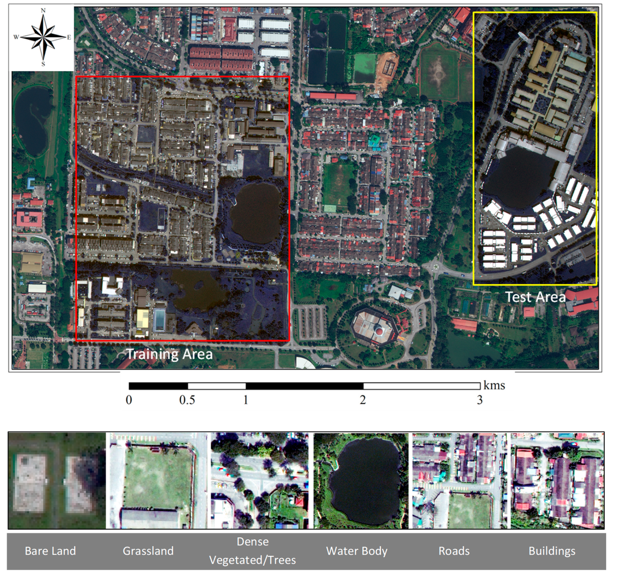
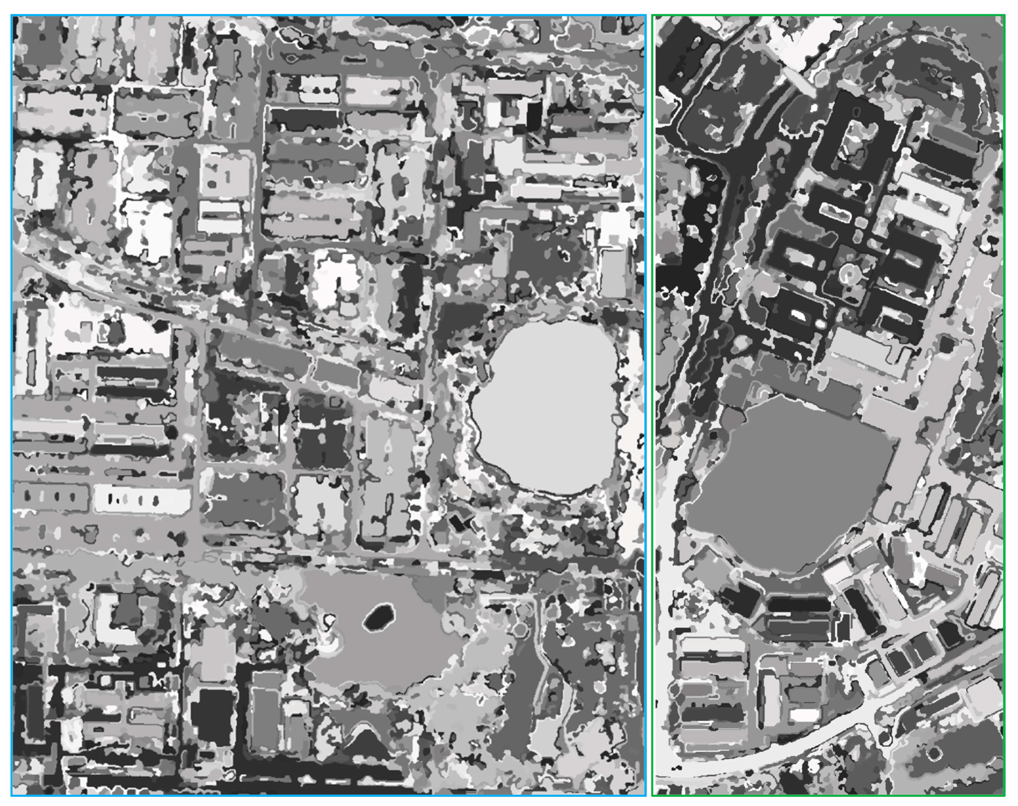
3. Study Area and Dataset
4. Methodology
4.1. Data Preprocessing
4.2. Image Segmentation
4.3. Object-Based Convolutional Neural Networks (OCNN)
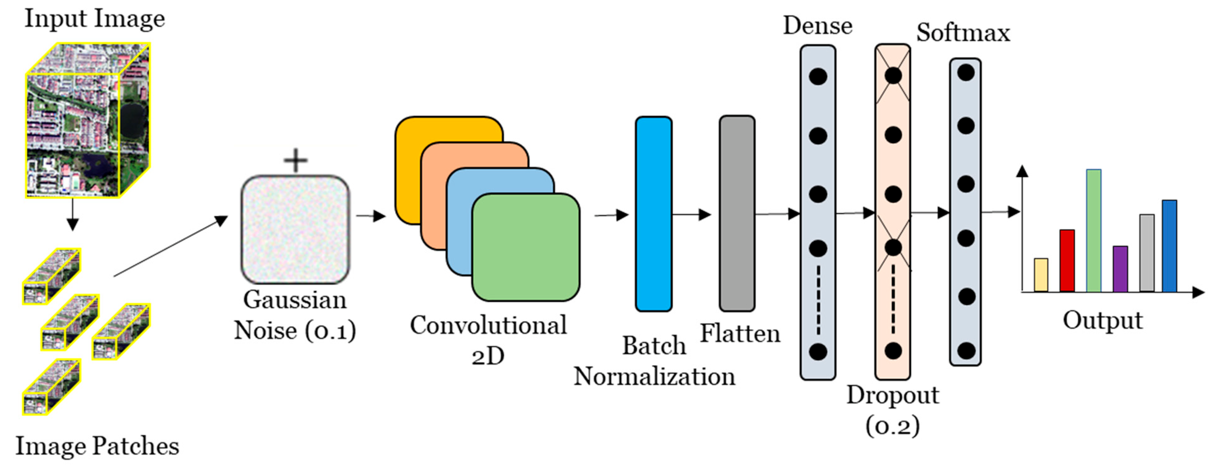
4.3.1. The Backbone Convolutional Neural Network (CNN)
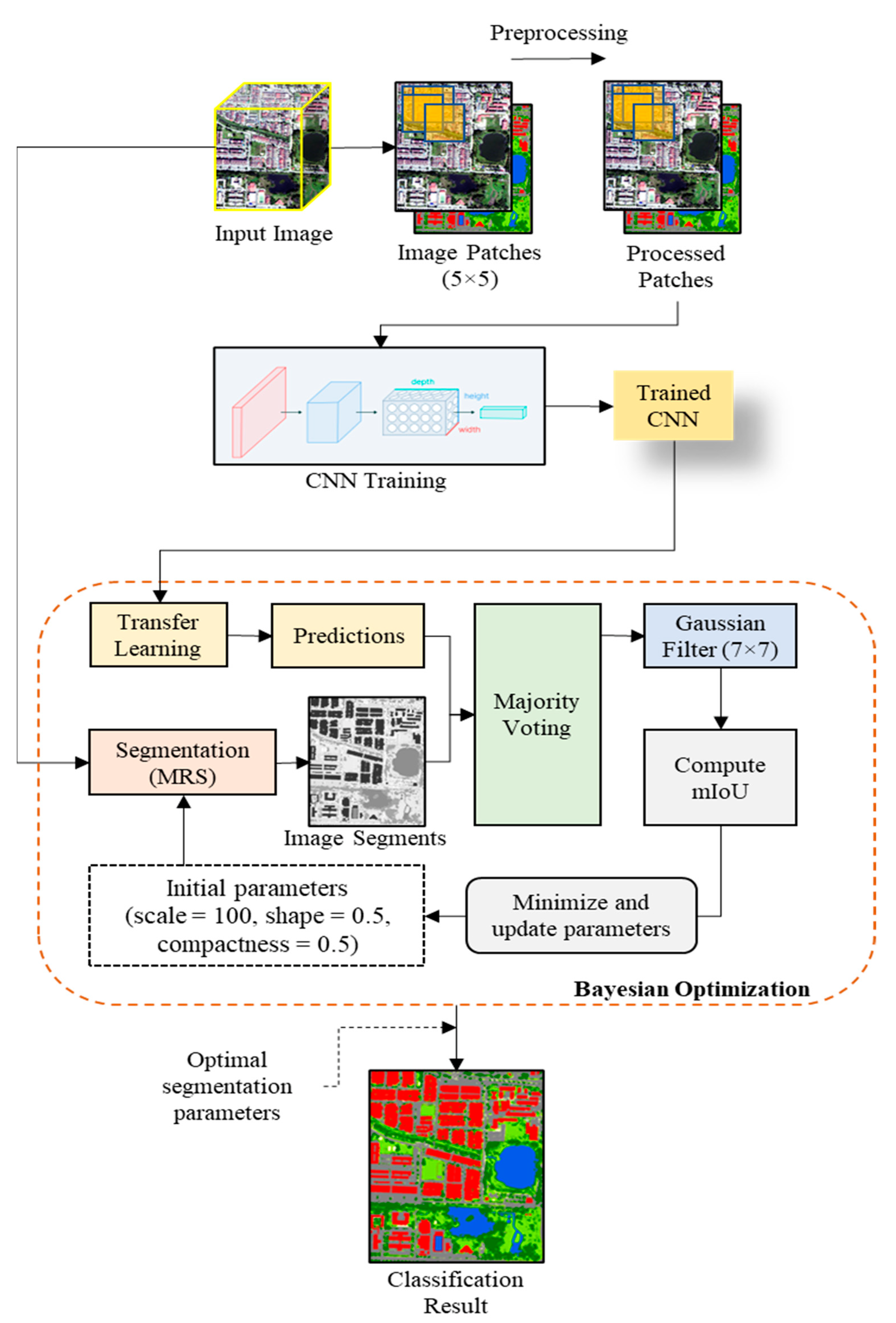
4.3.2. The Proposed OCNN Framework (OCNN-JO)
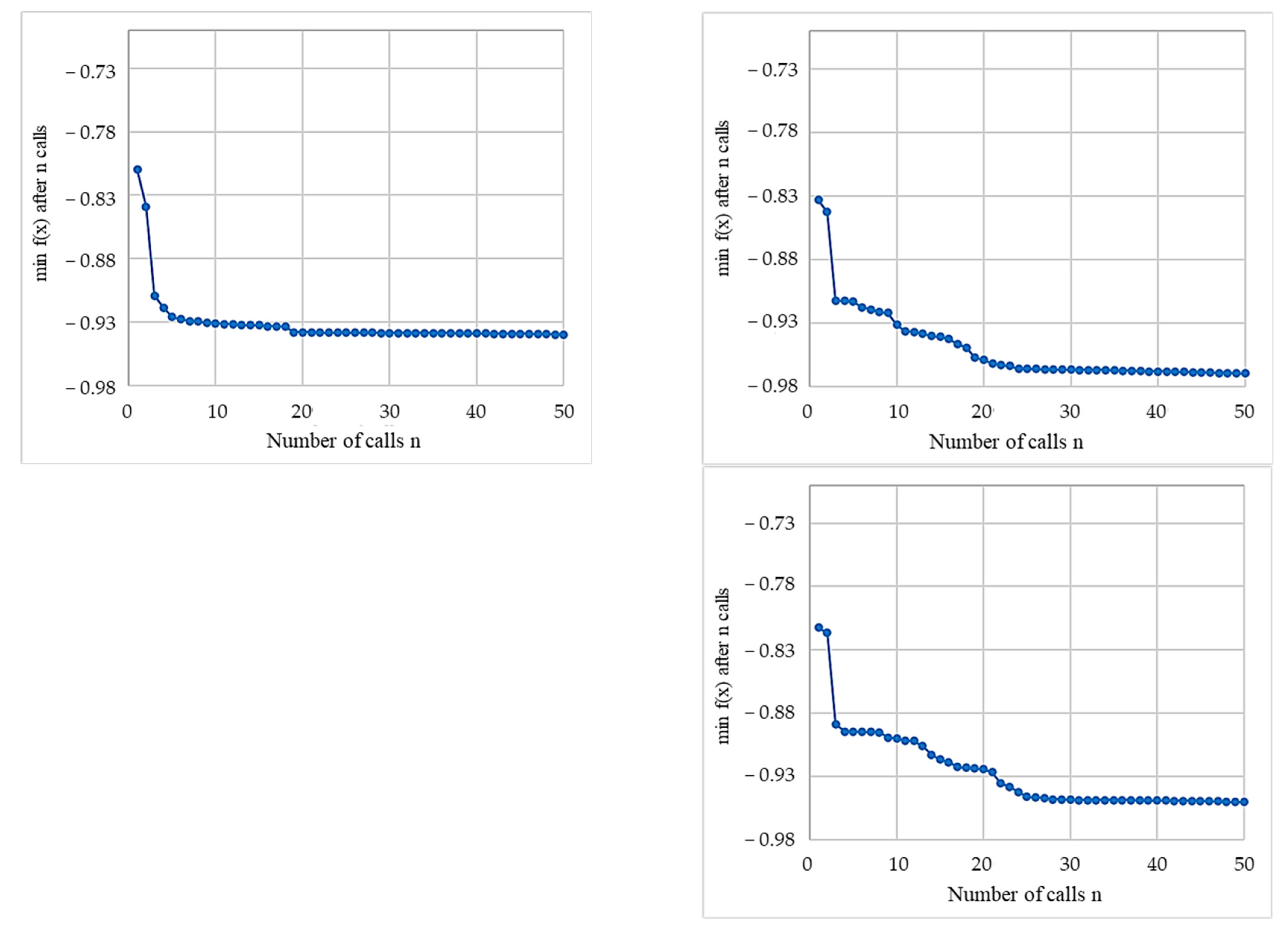
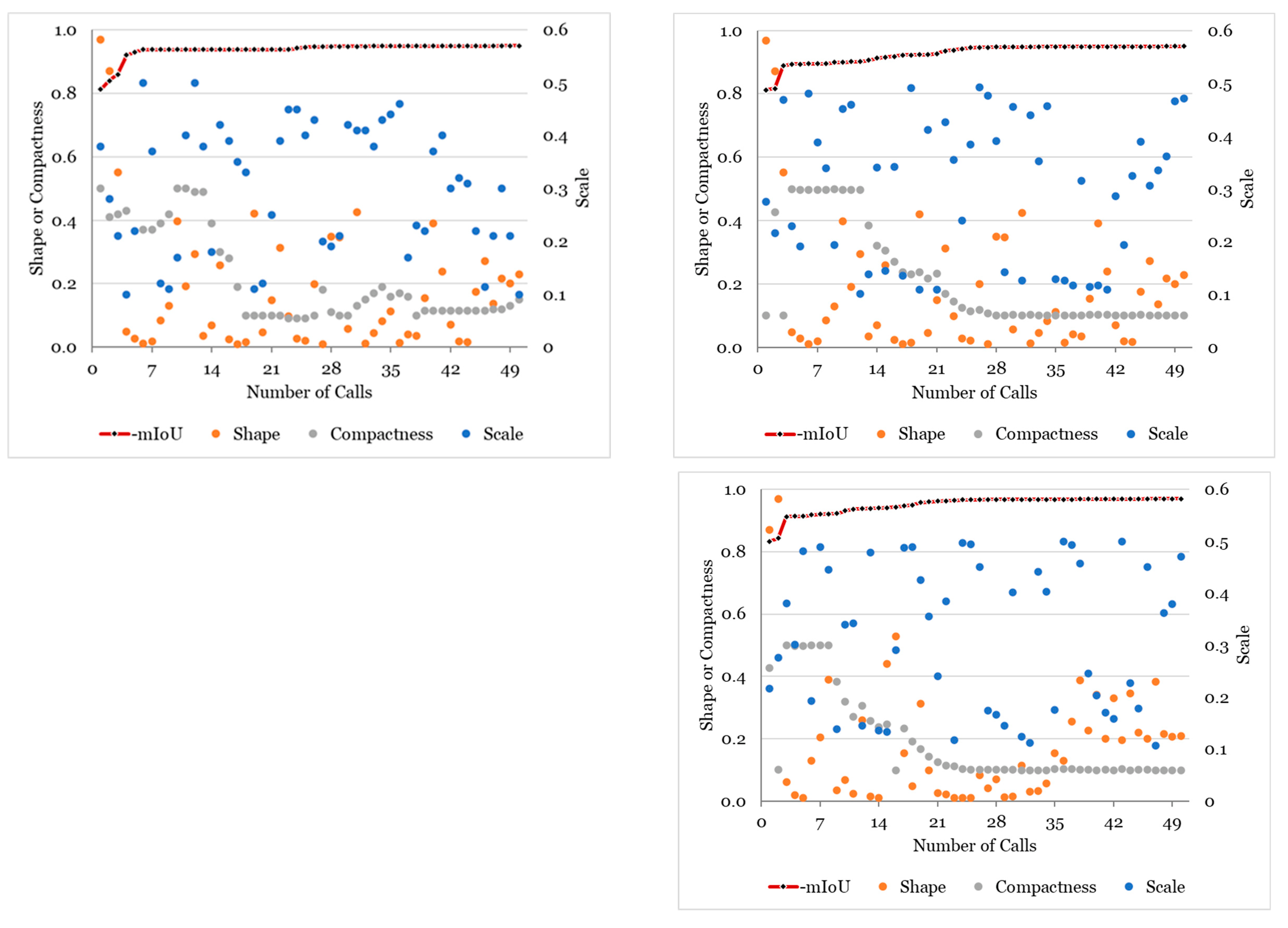
- Bayesian Optimization
- Transfer Learning
- Majority Voting
- Gaussian Filtering
- Training Strategy
4.4. Benchmark Methods
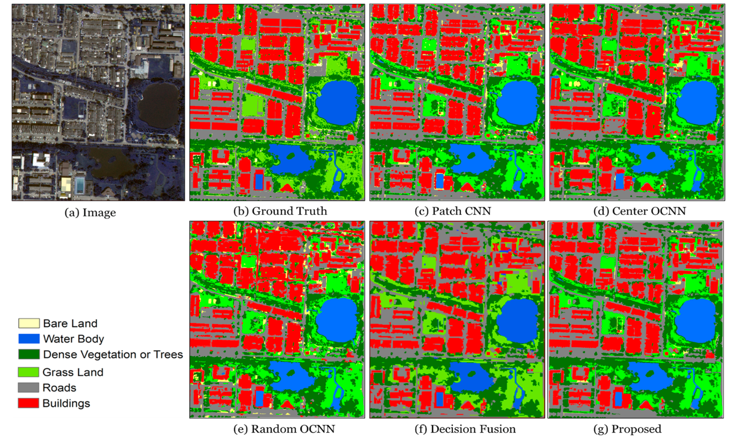
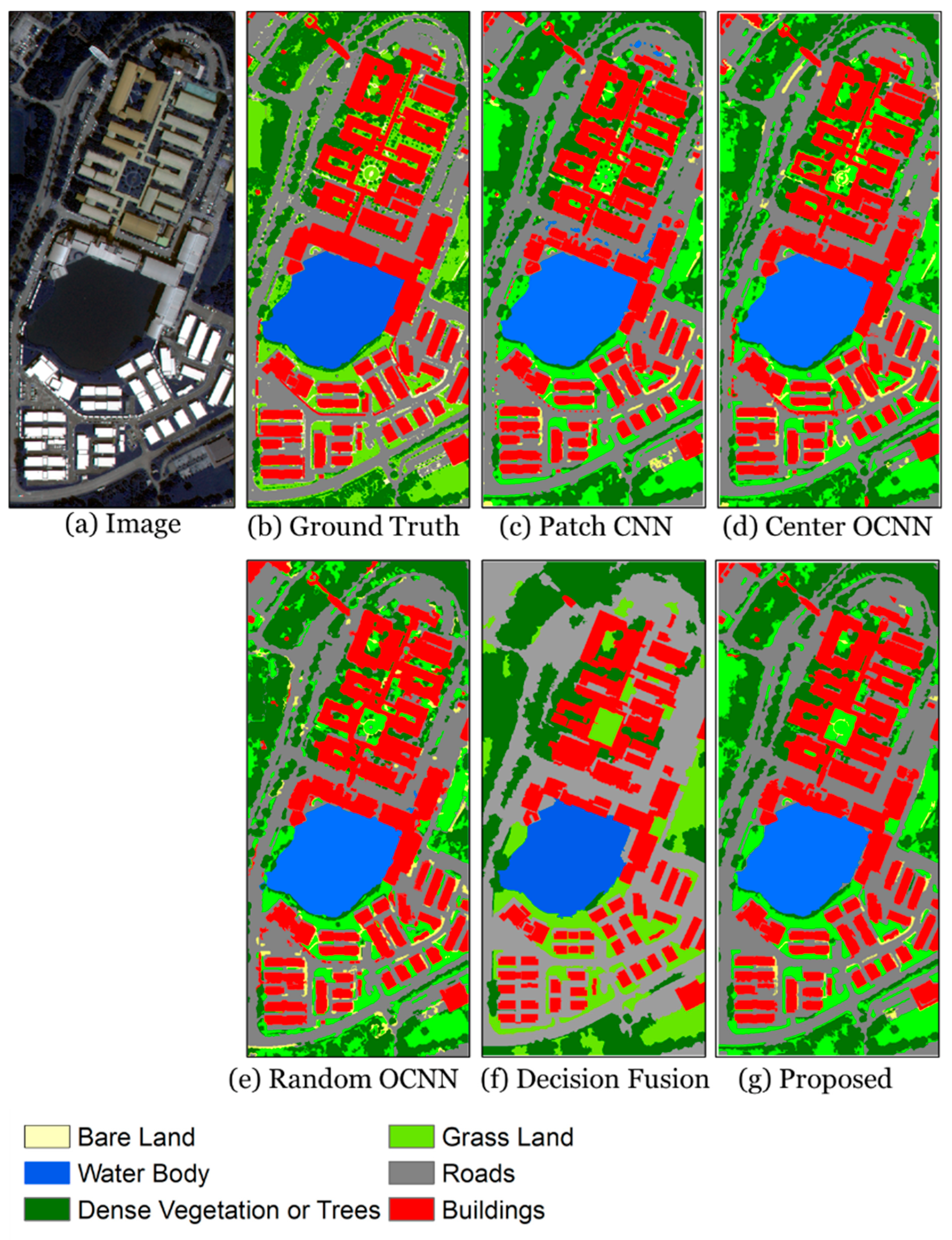
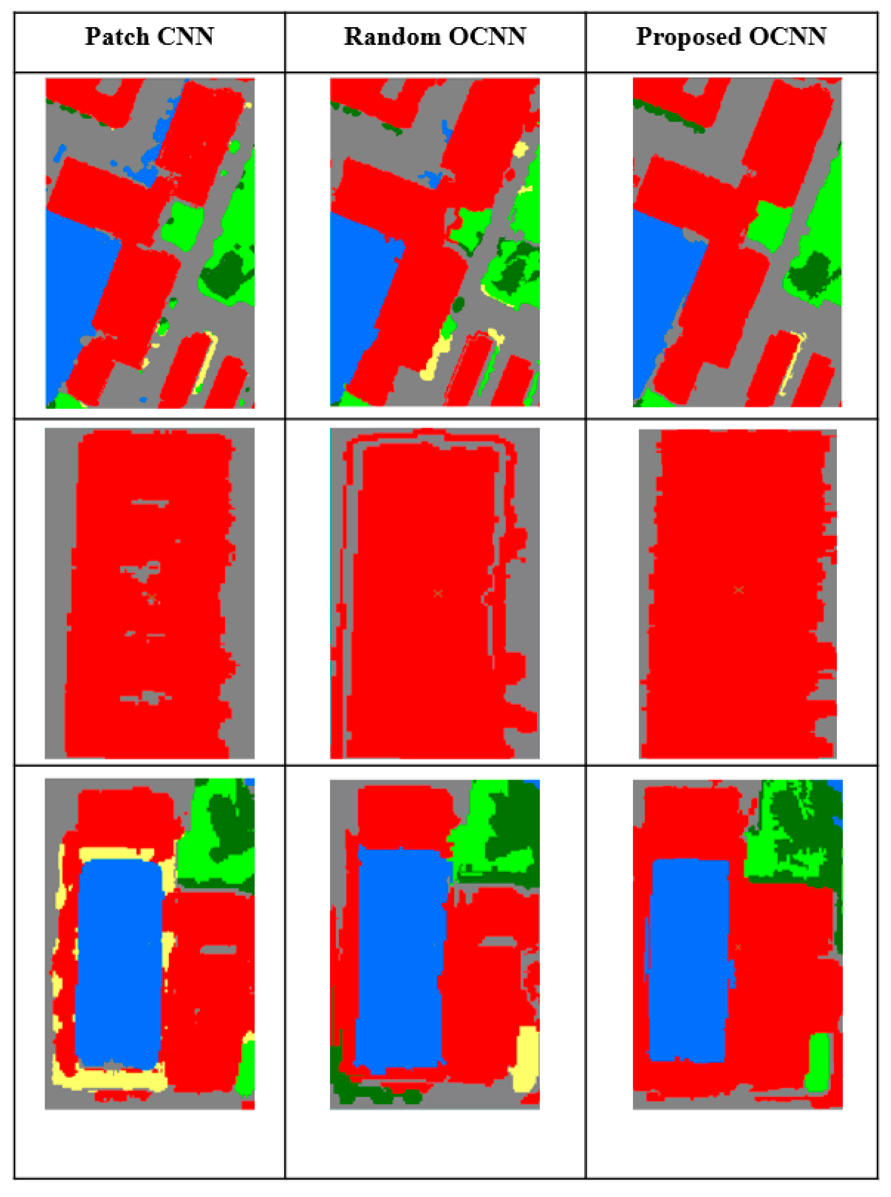
- Patch CNN: This model is based on densely overlapping patches with the size of a 9 × 9 set experimentally. The number of convolutional layers and their corresponding number of filters are also set experimentally to 2 and 64, respectively.
- Center-Point OCNN: In contrast to pixel-wise CNN, this model uses image segmentation to extract patches at the objects’ centers. The segmentation parameter scale, shape, and compactness were set experimentally to 4500, 0.15, and 0.1, respectively.
- RMV-OCNN: This model works principally as the CPOCNN; however, it randomly generates N convolutional positions within each image segment and trains the CNN. The same segmentation parameters are chosen for this model. The network’s architecture and hyperparameters are also identical to the CPOCNN.
- Decision-Fusion OCNN: This model generates predictions for each image pixel within image segments by using the PCNN and subsequently fuses them with a majority voting strategy to achieve the final classification results.
4.5. Accuracy Assessment
4.5.1. Classification Accuracy Assessment
4.5.2. Segmentation Quality Assessment
5. Results and Discussions
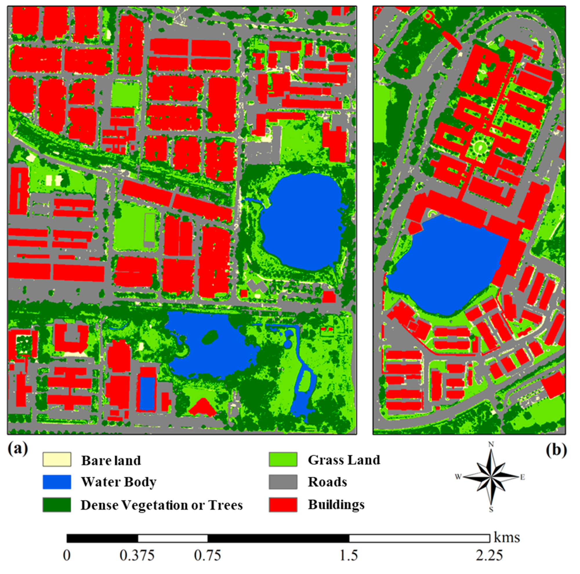
5.1. Segmentation Results
5.2. The Results of the Proposed Model
5.3. Performance Comparison with Benchmark Models
5.4. Sensitivity Analysis
5.4.1. Sensitivity Analysis of the Segmentation Parameters
5.4.2. The Effect of Patch Size
5.4.3. Computational Efficiency
5.5. Discussion
6. Conclusions
- Bayesian optimization could find comparable optimal MRS parameters for the training and testing areas with excellent quality measured by AFI (0.046, −0.037) and QR (0.945, 0.932). The best scales were 4705 and 4617 for the training and test areas, respectively. The best shape and compactness values were 0.2 and 0.1 for the training area and 0.14 and 0.1 for the test area.
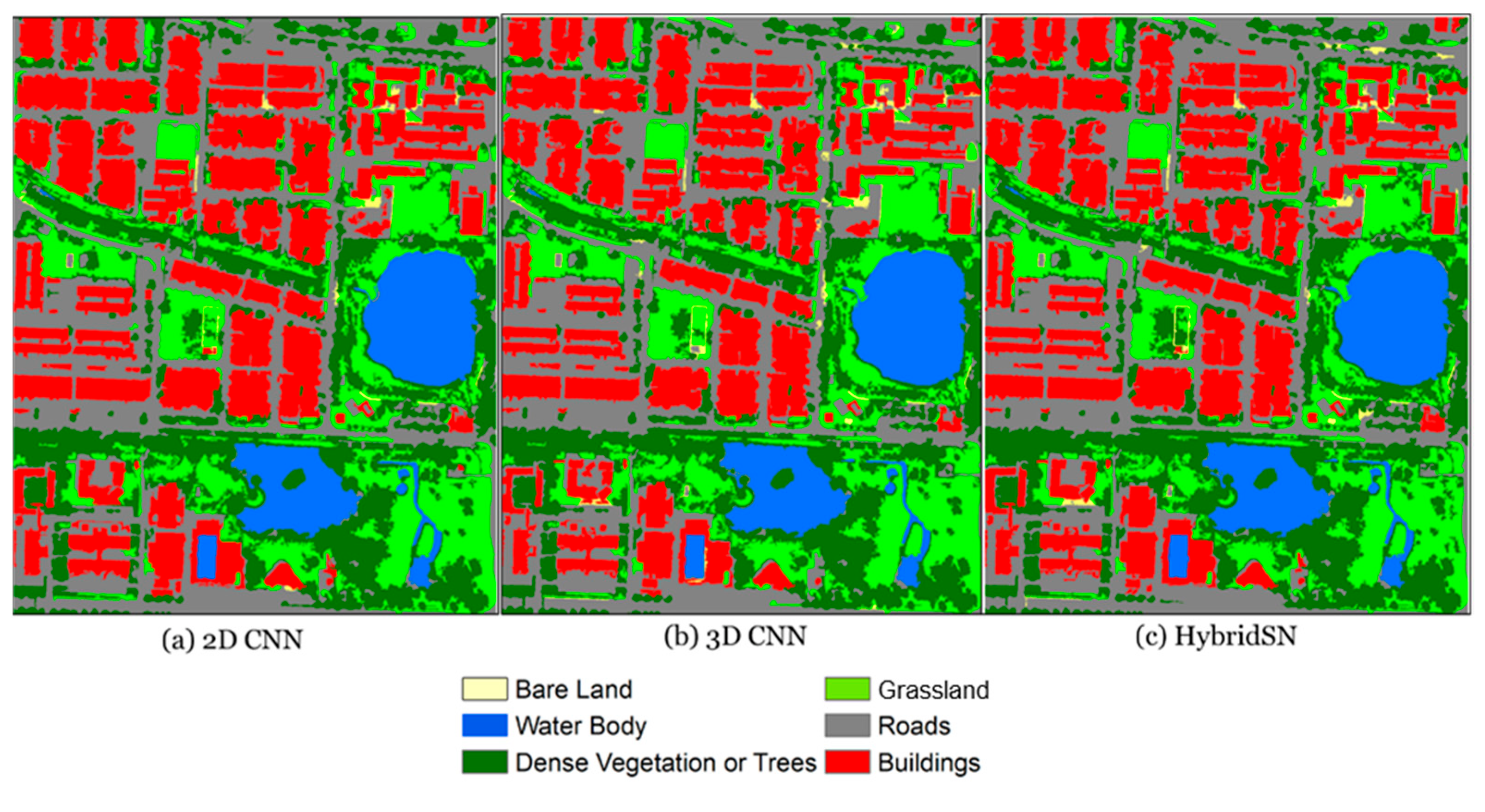
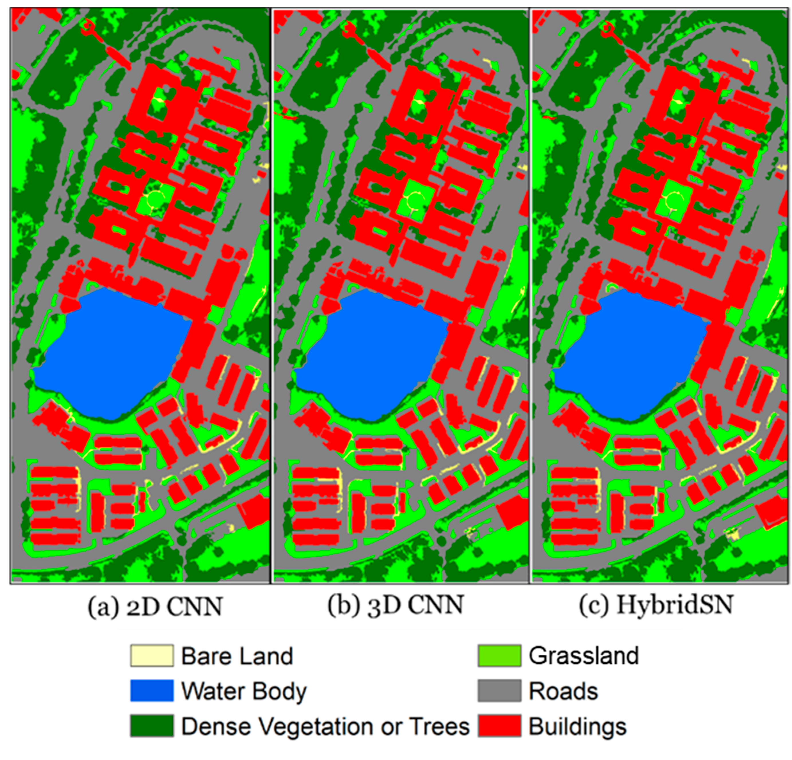
- For the proposed classification workflow, the HybridSN model achieved the best results compared to 2D and 3D CNNs. In the training area, the HybridSN model achieved 0.96 OA and mIoU and 0.95 Kappa. Slightly better accuracies (0.97 OA and mIoU and 0.96 Kappa) were obtained for this model in the test area. The 3D CNN layers and combining 3D and 2D CNN layers (HybridSN) yielded slightly better accuracies than the 2D CNN layers regarding geometric fidelity, object boundary extraction, and separation of adjacent objects.
- A comparison of the proposed model with several benchmark methods showed that the proposed model achieved the highest accuracy, reaching 0.96 OA, 0.95 Kappa, and 0.96 mIoU in the training area and 0.97 OA, 0.96 Kappa, and 0.97 mIoU in the test area.
- Sensitivity analysis on patch size used for CNN showed that higher accuracies could be obtained with larger patch sizes and the largest patch size (9 × 9) achieved accuracies as high as 0.94 for 2D CNN, 0.95 for 3D CNN, and 0.97 for HybridSN.
- The computational efficiency assessment of the presented model and the implemented benchmark methods showed that all the methods could be trained on a normal computer with no GPU in a relatively short time (<25 s for the most complex model).
Author Contributions
Funding
Data Availability Statement
Acknowledgments
Conflicts of Interest
References
- Chen, B.; Xu, B.; Gong, P. Mapping essential urban land use categories (EULUC) using geospatial big data: Progress, challenges, and opportunities. Big Earth Data 2021, 5, 410–441. [Google Scholar] [CrossRef]
- Pauleit, S.; Ennos, R.; Golding, Y. Modeling the environmental impacts of urban land use and land cover change—A study in Merseyside, UK. Landsc. Urban Plan 2005, 71, 295–310. [Google Scholar] [CrossRef]
- Zhang, C.; Sargent, I.; Pan, X.; Li, H.; Gardiner, A.; Hare, J.; Atkinson, P.M. An object-based convolutional neural network (OCNN) for urban land use classification. Remote Sens. Environ. 2018, 216, 57–70. [Google Scholar] [CrossRef] [Green Version]
- Zhang, P.; Ke, Y.; Zhang, Z.; Wang, M.; Li, P.; Zhang, S. Urban Land Use and Land Cover Classification Using Novel Deep Learning Models Based on High Spatial Resolution Satellite Imagery. Sensors 2018, 18, 3717. [Google Scholar] [CrossRef] [PubMed] [Green Version]
- Pesaresi, M.; Huadong, G.; Blaes, X.; Ehrlich, D.; Ferri, S.; Gueguen, L.; Halkia, M.; Kauffmann, M.; Kemper, T.; Lu, L.; et al. A Global Human Settlement Layer from Optical HR/VHR RS Data: Concept and First Results. IEEE J. Sel. Top. Appl. Earth Observ. Remote Sens. 2013, 6, 2102–2131. [Google Scholar] [CrossRef]
- Pan, G.; Qi, G.; Wu, Z.; Zhang, D.; Li, S. Land-Use Classification Using Taxi GPS Traces. IEEE Trans. Intell. Transp. Syst. 2013, 14, 113–123. [Google Scholar] [CrossRef]
- Zhu, Q.; Lei, Y.; Sun, X.; Guan, Q.; Zhong, Y.; Zhang, L.; Li, D. Knowledge-guided land pattern depiction for urban land use mapping: A case study of Chinese cities. Remote Sens. Environ. 2022, 272, 112916. [Google Scholar] [CrossRef]
- Zhang, T.; Su, J.; Xu, Z.; Luo, Y.; Li, J. Sentinel-2 Satellite Imagery for Urban Land Cover Classification by Optimized Random Forest Classifier. Appl. Sci. 2021, 11, 543. [Google Scholar] [CrossRef]
- Jozdani, S.E.; Johnson, B.A.; Chen, D. Comparing Deep Neural Networks, Ensemble Classifiers, and Support Vector Machine Algorithms for Object-Based Urban Land Use/Land Cover Classification. Remote Sens. 2019, 11, 1713. [Google Scholar] [CrossRef] [Green Version]
- Zhang, C.; Sargent, I.; Pan, X.; Li, H.; Gardiner, A.; Hare, J.; Atkinson, P.M. Joint Deep Learning for land cover and land use classification. Remote Sens. Environ. 2018, 221, 173–187. [Google Scholar] [CrossRef]
- Xu, Y.; Du, B.; Zhang, L.; Cerra, D.; Pato, M.; Carmona, E.; Prasad, S.; Yokoya, N.; Hansch, R.; Le Saux, B. Advanced Multi-Sensor Optical Remote Sensing for Urban Land Use and Land Cover Classification: Outcome of the 2018 IEEE GRSS Data Fusion Contest. IEEE J. Sel. Top. Appl. Earth Obs. Remote Sens. 2019, 12, 1709–1724. [Google Scholar] [CrossRef]
- Huang, B.; Zhao, B.; Song, Y. Urban land-use mapping using a deep convolutional neural network with high spatial resolution multispectral remote sensing imagery. Remote Sens. Environ. 2018, 214, 73–86. [Google Scholar] [CrossRef]
- Shendryk, Y.; Rist, Y.; Ticehurst, C.; Thorburn, P. Deep learning for multi-modal classification of cloud, shadow and land cover scenes in PlanetScope and Sentinel-2 imagery. ISPRS J. Photogramm. Remote Sens. 2019, 157, 124–136. [Google Scholar] [CrossRef]
- Wang, C.; Shu, Q.; Wang, X.; Guo, B.; Liu, P.; Li, Q. A random forest classifier based on pixel comparison features for urban LiDAR data. ISPRS J. Photogramm. Remote Sens. 2018, 148, 75–86. [Google Scholar] [CrossRef]
- Herold, M.; Couclelis, H.; Clarke, K.C. The role of spatial metrics in the analysis and modeling of urban land use change. Comput. Environ. Urban. Syst. 2005, 29, 369–399. [Google Scholar] [CrossRef]
- Blaschke, T. Object based image analysis for remote sensing. ISPRS J. Photogramm. Remote Sens. 2010, 65, 2–16. [Google Scholar] [CrossRef] [Green Version]
- Lv, X.; Shao, Z.; Ming, D.; Diao, C.; Zhou, K.; Tong, C. Improved object-based convolutional neural network (IOCNN) to classify very high-resolution remote sensing images. Int. J. Remote Sens. 2021, 42, 8318–8344. [Google Scholar] [CrossRef]
- Li, H.; Zhang, C.; Zhang, Y.; Zhang, S.; Ding, X.; Atkinson, P.M. A Scale Sequence Object-based Convolutional Neural Network (SS-OCNN) for crop classification from fine spatial resolution remotely sensed imagery. Int. J. Digit. Earth 2021, 14, 1528–1546. [Google Scholar] [CrossRef]
- Chen, Y.; Tang, L.; Yang, X.; Bilal, M.; Li, Q. Object-based multi-modal convolution neural networks for building extraction using panchromatic and multispectral imagery. Neurocomputing 2019, 386, 136–146. [Google Scholar] [CrossRef]
- Rajesh, S.; Nisia, T.G.; Arivazhagan, S.; Abisekaraj, R. Land Cover/Land Use Mapping of LISS IV Imagery Using Object-Based Convolutional Neural Network with Deep Features. J. Indian Soc. Remote Sens. 2019, 48, 145–154. [Google Scholar] [CrossRef]
- Zhao, W.; Du, S.; Emery, W.J. Object-Based Convolutional Neural Network for High-Resolution Imagery Classification. IEEE J. Sel. Top. Appl. Earth Obs. Remote. Sens. 2017, 10, 3386–3396. [Google Scholar] [CrossRef]
- Blaschke, T.; Hay, G.J.; Kelly, M.; Lang, S.; Hofmann, P.; Addink, E.; Feitosa, R.Q.; van der Meer, F.; van der Werff, H.; van Coillie, F.; et al. Geographic Object-Based Image Analysis—Towards a new paradigm. ISPRS J. Photogramm. Remote Sens. 2014, 87, 180–191. [Google Scholar] [CrossRef] [PubMed] [Green Version]
- Rastner, P.; Bolch, T.; Notarnicola, C.; Paul, F. A Comparison of Pixel- and Object-Based Glacier Classification With Optical Satellite Images. IEEE J. Sel. Top. Appl. Earth Obs. Remote Sens. 2013, 7, 853–862. [Google Scholar] [CrossRef]
- Mayr, A.; Klambauer, G.; Unterthiner, T.; Steijaert, M.; Wegner, J.K.; Ceulemans, H.; Clevert, D.-A.; Hochreiter, S. Large-scale comparison of machine learning methods for drug target prediction on ChEMBL. Chem. Sci. 2018, 9, 5441–5451. [Google Scholar] [CrossRef] [PubMed] [Green Version]
- Gorishniy, Y.; Rubachev, I.; Khrulkov, V.; Babenko, A. Revisiting deep learning models for tabular data. Adv. Neural Inf. Process. Syst. 2021, 34, 18932–18943. [Google Scholar]
- Schäfl, B.; Gruber, L.; Bitto-Nemling, A.; Hochreiter, S. Hopular: Modern Hopfield Networks for Tabular Data. arXiv 2022, arXiv:2206.00664. [Google Scholar]
- Shwartz-Ziv, R.; Armon, A. Tabular data: Deep learning is not all you need. Inf. Fusion 2022, 81, 84–90. [Google Scholar] [CrossRef]
- Abdollahi, A.; Pradhan, B.; Shukla, N. Road Extraction from High-Resolution Orthophoto Images Using Convolutional Neural Network. J. Indian Soc. Remote Sens. 2020, 49, 569–583. [Google Scholar] [CrossRef]
- Lam, O.H.Y.; Dogotari, M.; Prüm, M.; Vithlani, H.N.; Roers, C.; Melville, B.; Zimmer, F.; Becker, R. An open source workflow for weed mapping in native grassland using unmanned aerial vehicle: Using Rumex obtusifolius as a case study. Eur. J. Remote Sens. 2020, 54, 71–88. [Google Scholar] [CrossRef]
- Attaf, D.; Djerriri, K.; Cheriguene, R.S.; Karoui, M.S. One-dimensional convolution neural networks for object-based feature selection. Proc. SPIE 2018, 10789, 107891N. [Google Scholar] [CrossRef]
- Majd, R.D.; Momeni, M.; Moallem, P. Transferable Object-Based Framework Based on Deep Convolutional Neural Networks for Building Extraction. IEEE J. Sel. Top. Appl. Earth Obs. Remote Sens. 2019, 12, 2627–2635. [Google Scholar] [CrossRef]
- Li, H.; Zhang, C.; Atkinson, P.M. A hybrid OSVM-OCNN Method for Crop Classification from Fine Spatial Resolution Remotely Sensed Imagery. Remote Sens. 2019, 11, 2370. [Google Scholar] [CrossRef]
- Sutha, J. Object based classification of high resolution remote sensing image using HRSVM-CNN classifier. Eur. J. Remote Sens. 2019, 53, 16–30. [Google Scholar] [CrossRef] [Green Version]
- Hong, L.; Zhang, M. Object-oriented multiscale deep features for hyperspectral image classification. Int. J. Remote Sens. 2020, 41, 5549–5572. [Google Scholar] [CrossRef]
- Tang, Z.; Li, M.; Wang, X. Mapping Tea Plantations from VHR Images Using OBIA and Convolutional Neural Networks. Remote Sens. 2020, 12, 2935. [Google Scholar] [CrossRef]
- Guirado, E.; Blanco-Sacristán, J.; Rodríguez-Caballero, E.; Tabik, S.; Alcaraz-Segura, D.; Martínez-Valderrama, J.; Cabello, J. Mask R-CNN and OBIA Fusion Improves the Segmentation of Scattered Vegetation in Very High-Resolution Optical Sensors. Sensors 2021, 21, 320. [Google Scholar] [CrossRef]
- Liu, S.; Qi, Z.; Li, X.; Yeh, A.G.-O. Integration of Convolutional Neural Networks and Object-Based Post-Classification Refinement for Land Use and Land Cover Mapping with Optical and SAR Data. Remote Sens. 2019, 11, 690. [Google Scholar] [CrossRef] [Green Version]
- Abdi, G.; Samadzadegan, F.; Reinartz, P. Deep learning decision fusion for the classification of urban remote sensing data. J. Appl. Remote Sens. 2018, 12, 016038. [Google Scholar] [CrossRef]
- Robson, B.A.; Bolch, T.; MacDonell, S.; Hölbling, D.; Rastner, P.; Schaffer, N. Automated detection of rock glaciers using deep learning and object-based image analysis. Remote Sens. Environ. 2020, 250, 112033. [Google Scholar] [CrossRef]
- Timilsina, S.; Aryal, J.; Kirkpatrick, J. Mapping Urban Tree Cover Changes Using Object-Based Convolution Neural Network (OB-CNN). Remote Sens. 2020, 12, 3017. [Google Scholar] [CrossRef]
- He, S.; Du, H.; Zhou, G.; Li, X.; Mao, F.; Zhu, D.E.; Xu, Y.; Zhang, M.; Huang, Z.; Liu, H.; et al. Intelligent mapping of urban forests from high-resolution remotely sensed imagery using object-based u-net-densenet-coupled network. Remote Sens. 2020, 12, 3928. [Google Scholar] [CrossRef]
- Bengoufa, S.; Niculescu, S.; Mihoubi, M.K.; Belkessa, R.; Abbad, K. Rocky shoreline extraction using a deep learning model and object-based image analysis. ISPRS Int. Arch. Photogramm. Remote Sens. Spat. Inf. Sci. 2021, XLIII-B3-2, 23–29. [Google Scholar] [CrossRef]
- Martins, V.S.; Kaleita, A.L.; Gelder, B.K.; da Silveira, H.L.; Abe, C.A. Exploring multiscale object-based convolutional neural network (multi-OCNN) for remote sensing image classification at high spatial resolution. ISPRS J. Photogramm. Remote Sens. 2020, 168, 56–73. [Google Scholar] [CrossRef]
- Pan, X.; Zhao, J.; Xu, J. An object-based and heterogeneous segment filter convolutional neural network for high-resolution remote sensing image classification. Int. J. Remote Sens. 2019, 40, 5892–5916. [Google Scholar] [CrossRef]
- Wang, J.; Zheng, Y.; Wang, M.; Shen, Q.; Huang, J. Object-Scale Adaptive Convolutional Neural Networks for High-Spatial Resolution Remote Sensing Image Classification. IEEE J. Sel. Top. Appl. Earth Obs. Remote Sens. 2020, 14, 283–299. [Google Scholar] [CrossRef]
- Russ, J.C. The Image Processing Handbook; CRC Press: Boca Raton, FL, USA, 2006; p. 832. [Google Scholar]
- Atik, S.; Ipbuker, C. Integrating Convolutional Neural Network and Multiresolution Segmentation for Land Cover and Land Use Mapping Using Satellite Imagery. Appl. Sci. 2021, 11, 5551. [Google Scholar] [CrossRef]
- Lourenço, P.; Teodoro, A.; Gonçalves, J.; Honrado, J.; Cunha, M.; Sillero, N. Assessing the performance of different OBIA software approaches for mapping invasive alien plants along roads with remote sensing data. Int. J. Appl. earth Obs. Geoinf. ITC J. 2020, 95, 102263. [Google Scholar] [CrossRef]
- Zhou, T.; Fu, H.; Sun, C.; Wang, S. Shadow Detection and Compensation from Remote Sensing Images under Complex Urban Conditions. Remote Sens. 2021, 13, 699. [Google Scholar] [CrossRef]
- Xue, Y.; Zhao, J.; Zhang, M. A Watershed-Segmentation-Based Improved Algorithm for Extracting Cultivated Land Boundaries. Remote Sens. 2021, 13, 939. [Google Scholar] [CrossRef]
- Dawei, L.; Shujing, G. Object Oriented Road Extraction from Remote Sensing Images Using Improved Watershed Segmentation. J. Phys. Conf. Ser. 2021, 2005, 012077. [Google Scholar] [CrossRef]
- Li, Y.; Ouyang, S.; Zhang, Y. Combining deep learning and ontology reasoning for remote sensing image semantic segmentation. Knowl. Based Syst. 2022, 243, 108469. [Google Scholar] [CrossRef]
- Baatz, M. Multi resolution segmentation: An optimum approach for high quality multi scale image segmentation. In Beutrage zum AGIT-Symposium; Salzburg: Heidelberg, Germany, 2000; pp. 12–23. [Google Scholar]
- Hossain, M.D.; Chen, D. Segmentation for Object-Based Image Analysis (OBIA): A review of algorithms and challenges from remote sensing perspective. ISPRS J. Photogramm. Remote Sens. 2019, 150, 115–134. [Google Scholar] [CrossRef]
- Chen, T.; Trinder, J.C.; Niu, R. Object-Oriented Landslide Mapping Using ZY-3 Satellite Imagery, Random Forest and Mathematical Morphology, for the Three-Gorges Reservoir, China. Remote Sens. 2017, 9, 333. [Google Scholar] [CrossRef] [Green Version]
- Definiens, A.G. Definiens Professional 5 User Guide; Definiens AG: Munich, Germany, 2006. [Google Scholar]
- Munyati, C. Optimising multiresolution segmentation: Delineating savannah vegetation boundaries in the Kruger National Park, South Africa, using Sentinel 2 MSI imagery. Int. J. Remote Sens. 2018, 39, 5997–6019. [Google Scholar] [CrossRef]
- Shahabi, H.; Jarihani, B.; Piralilou, S.T.; Chittleborough, D.; Avand, M.; Ghorbanzadeh, O. A Semi-Automated Object-Based Gully Networks Detection Using Different Machine Learning Models: A Case Study of Bowen Catchment, Queensland, Australia. Sensors 2019, 19, 4893. [Google Scholar] [CrossRef] [Green Version]
- Fu, T.; Ma, L.; Li, M.; Johnson, B.A. Using convolutional neural network to identify irregular segmentation objects from very high-resolution remote sensing imagery. J. Appl. Remote Sens. 2018, 12, 025010. [Google Scholar] [CrossRef]
- Strigl, D.; Kofler, K.; Podlipnig, S. Performance and Scalability of GPU-Based Convolutional Neural Networks. In Proceedings of the 2010 18th Euromicro Conference on Parallel, Distributed and Network-based Processing, Pisa, Italy, 17–19 February 2010; pp. 317–324. [Google Scholar]
- Schmidhuber, J. Deep Learning in Neural Networks: An Overview. Neural Netw. 2015, 61, 85–117. [Google Scholar] [CrossRef] [Green Version]
- Lee, T.; Lee, K.B.; Kim, C.O. Performance of Machine Learning Algorithms for Class-Imbalanced Process Fault Detection Problems. IEEE Trans. Semicond. Manuf. 2016, 29, 436–445. [Google Scholar] [CrossRef]
- Brochu, E.; Cora, V.M.; De Freitas, N. A tutorial on Bayesian optimization of expensive cost functions, with application to active user modeling and hierarchical reinforcement learning. arXiv 2020, arXiv:1012.2599. [Google Scholar]
- Frazier, P.I. A tutorial on Bayesian optimization. arXiv 2018, arXiv:1807.02811. [Google Scholar]
- Shahriari, B.; Swersky, K.; Wang, Z.; Adams, R.P.; de Freitas, N. Taking the Human Out of the Loop: A Review of Bayesian Optimization. Proc. IEEE 2015, 104, 148–175. [Google Scholar] [CrossRef] [Green Version]
- Snoek, J.; Larochelle, H.; Adams, R.P. Practical Bayesian optimization of machine learning algorithms. Adv. Neural Inf. Process Syst. 2012, 25. [Google Scholar]
- Rathbun, S.L.; Stein, M.L. Interpolation of Spatial Data: Some Theory for Kriging. J. Am. Stat. Assoc. 2000, 95, 1010. [Google Scholar] [CrossRef]
- Jones, D.R.; Schonlau, M.; Welch, W.J. Efficient Global Optimization of Expensive Black-Box Functions. J. Glob. Optim. 1998, 13, 455–492. [Google Scholar] [CrossRef]
- Kingma, D.P.; Ba, J. Adam: A method for stochastic optimization. arXiv 2014, arXiv:1412.6980. [Google Scholar]
- Zhang, X.; Han, L.; Zhu, L. How well do deep learning-based methods for land cover classification and object detection perform on high resolution remote sensing imagery? Remote Sens. 2020, 12, 417. [Google Scholar] [CrossRef]
- El-Naggar, A.M. Determination of optimum segmentation parameter values for extracting building from remote sensing images. Alex. Eng. J. 2018, 57, 3089–3097. [Google Scholar] [CrossRef]
- Paoletti, M.E.; Haut, J.M.; Plaza, J.; Plaza, A. A new deep convolutional neural network for fast hyperspectral image classification. ISPRS J. Photogramm. Remote Sens. 2018, 145, 120–147. [Google Scholar] [CrossRef]
- Kavzoğlu, T.; Yilmaz, E. Analysis of patch and sample size effects for 2D-3D CNN models using multiplatform dataset: Hyperspectral image classification of ROSIS and Jilin-1 GP01 imagery. Turk. J. Electr. Eng. Comput. Sci. 2022, 30, 2124–2144. [Google Scholar] [CrossRef]
- Nababan, B.; Mastu, L.O.K.; Idris, N.H.; Panjaitan, J.P. Shallow-Water Benthic Habitat Mapping Using Drone with Object Based Image Analyses. Remote Sens. 2021, 13, 4452. [Google Scholar] [CrossRef]
- Zaabar, N.; Niculescu, S.; Kamel, M.M. Application of Convolutional Neural Networks With Object-Based Image Analysis for Land Cover and Land Use Mapping in Coastal Areas: A Case Study in Ain Témouchent, Algeria. IEEE J. Sel. Top. Appl. Earth Obs. Remote Sens. 2022, 15, 5177–5189. [Google Scholar] [CrossRef]


| Land-Cover Class | Pixels | Percentage | ||
|---|---|---|---|---|
| Training Area | Test Area | Training Area | Test Area | |
| Buildings | 275,441 | 144,260 | 26.10% | 23.90% |
| Roads | 288,816 | 191,106 | 27.36% | 31.66% |
| Grassland | 168,018 | 87,707 | 15.92% | 14.53% |
| Dense Vegetation/Trees | 215,104 | 111,872 | 20.38% | 18.53% |
| Water Body | 85,762 | 54,183 | 8.13% | 8.98% |
| Bare Land | 22,284 | 14,469 | 2.11% | 2.40% |
| SUM | 1,055,425 | 603,597 | 100.00% | 100.00% |
| Parameter | Search Space | Initial Value | Best Value (Training Area) | Best Value (Test Area) |
|---|---|---|---|---|
| Scale | Integer [25, 5000] | 100 | 4705 | 4617 |
| Shape | Real [10−2, 100] | 0.5 | 0.2 | 0.14 |
| Compactness | Real [10−2, 100] | 0.5 | 0.1 | 0.1 |
| Dataset | AFI | QR |
|---|---|---|
| Training Area | 0.046 | 0.945 |
| Test Area | −0.037 | 0.932 |
| Training Area | Test Area | |||||
|---|---|---|---|---|---|---|
| Class | 2D CNN | 3D CNN | HybridSN | 2D CNN | 3D CNN | HybridSN |
| Buildings | 0.94 | 0.94 | 0.97 | 0.95 | 0.96 | 0.97 |
| Roads | 0.98 | 0.96 | 0.94 | 0.98 | 0.98 | 0.98 |
| Grass Land | 0.93 | 0.93 | 0.95 | 0.93 | 0.91 | 0.94 |
| Dense Vegetation/Trees | 0.93 | 0.96 | 0.94 | 0.9 | 0.91 | 0.95 |
| Water Body | 0.98 | 0.97 | 0.98 | 0.98 | 0.98 | 0.99 |
| Bare Land | 0.88 | 0.92 | 0.98 | 0.93 | 0.95 | 0.98 |
| OA | 0.94 | 0.95 | 0.96 | 0.94 | 0.95 | 0.97 |
| Kappa | 0.92 | 0.94 | 0.95 | 0.93 | 0.94 | 0.96 |
| mIoU | 0.94 | 0.95 | 0.96 | 0.94 | 0.95 | 0.97 |
| Class | Patch CNN | Center OCNN | Random OCNN | Decision Fusion | Proposed |
|---|---|---|---|---|---|
| Buildings | 0.85 | 0.96 | 0.85 | 0.84 | 0.97 |
| Roads | 0.85 | 0.87 | 0.83 | 0.83 | 0.94 |
| Grass Land | 0.91 | 0.95 | 0.94 | 0.8 | 0.95 |
| Dense Vegetation/Trees | 0.93 | 0.93 | 0.94 | 0.84 | 0.94 |
| Water Body | 0.96 | 0.98 | 0.98 | 0.93 | 0.98 |
| Bare Land | 0.93 | 0.98 | 0.98 | 0.89 | 0.98 |
| OA | 0.89 | 0.93 | 0.9 | 0.89 | 0.96 |
| Kappa | 0.86 | 0.91 | 0.87 | 0.88 | 0.95 |
| mIoU | 0.89 | 0.93 | 0.9 | 0.89 | 0.96 |
| Class | Patch CNN | Center OCNN | Random OCNN | Decision Fusion | Proposed |
|---|---|---|---|---|---|
| Buildings | 0.9 | 0.96 | 0.96 | 0.92 | 0.97 |
| Roads | 0.91 | 0.93 | 0.94 | 0.89 | 0.98 |
| Grass Land | 0.89 | 0.94 | 0.89 | 0.9 | 0.94 |
| Dense Vegetation/Trees | 0.96 | 0.96 | 0.93 | 0.94 | 0.95 |
| Water Body | 0.99 | 0.97 | 0.98 | 0.98 | 0.99 |
| Bare Land | 0.97 | 0.98 | 0.98 | 0.95 | 0.98 |
| OA | 0.93 | 0.95 | 0.94 | 0.93 | 0.97 |
| Kappa | 0.91 | 0.94 | 0.9 | 0.92 | 0.96 |
| mIoU | 0.93 | 0.95 | 0.93 | 0.93 | 0.97 |
| Patch Size | mIoU | ||
|---|---|---|---|
| 2D CNN | 3D CNN | HybridSN | |
| 3 | 0.93 | 0.94 | 0.95 |
| 5 | 0.93 | 0.94 | 0.95 |
| 7 | 0.94 | 0.95 | 0.96 |
| 9 | 0.94 | 0.95 | 0.97 |
| Model | Base CNN | Segmentation (s) | Data Preparation and Preprocessing (s) | Training Time (s/epoch) | Post-Processing Time (s) | Total (s) |
|---|---|---|---|---|---|---|
| Patch CNN | 2D CNN | - | 5.3 | 2.27 | 0 | 7.57 |
| Center OCNN | 2D CNN | 2 | 17.66 | 0.001 | 2 | 21.661 |
| Random OCNN | 2D CNN | 2 | 15.61 | 0.003 | 3 | 20.613 |
| Decision Fusion | 2D CNN | 2 | 5.3 | 2.27 | 3 | 12.57 |
| Proposed | 2D CNN | 2 | 5.3 | 2.27 | 5 | 10.57 |
| Proposed | 3D CNN | 2 | 5.5 | 11.13 | 5 | 23.63 |
| Proposed | HybridSN | 2 | 5.5 | 12.14 | 5 | 24.64 |
| Bayesian Optimization (per iteration) | - | - | - | 13 | - | 13 |
Publisher’s Note: MDPI stays neutral with regard to jurisdictional claims in published maps and institutional affiliations. |
© 2022 by the authors. Licensee MDPI, Basel, Switzerland. This article is an open access article distributed under the terms and conditions of the Creative Commons Attribution (CC BY) license (https://creativecommons.org/licenses/by/4.0/).
Share and Cite
Azeez, O.S.; Shafri, H.Z.M.; Alias, A.H.; Haron, N.A. A Joint Bayesian Optimization for the Classification of Fine Spatial Resolution Remotely Sensed Imagery Using Object-Based Convolutional Neural Networks. Land 2022, 11, 1905. https://doi.org/10.3390/land11111905
Azeez OS, Shafri HZM, Alias AH, Haron NA. A Joint Bayesian Optimization for the Classification of Fine Spatial Resolution Remotely Sensed Imagery Using Object-Based Convolutional Neural Networks. Land. 2022; 11(11):1905. https://doi.org/10.3390/land11111905
Chicago/Turabian StyleAzeez, Omer Saud, Helmi Z. M. Shafri, Aidi Hizami Alias, and Nuzul Azam Haron. 2022. "A Joint Bayesian Optimization for the Classification of Fine Spatial Resolution Remotely Sensed Imagery Using Object-Based Convolutional Neural Networks" Land 11, no. 11: 1905. https://doi.org/10.3390/land11111905