Article

Estimating Precipitation Using LSTM-Based Raindrop Spectrum in Guizhou

1
College of Electronic Engineering, Chengdu University of Information Technology, Chengdu 610225, China
2
Key Laboratory of Land Surface Process and Climate Change in Cold and Arid Regions, Chinese Academy of Sciences, Lanzhou 730000, China
*
Author to whom correspondence should be addressed.
Atmosphere 2023, 14(6), 1031; https://doi.org/10.3390/atmos14061031
Submission received: 20 April 2023 / Revised: 25 May 2023 / Accepted: 10 June 2023 / Published: 15 June 2023

Abstract

:
The change in raindrop spectrum characteristics is an important factor affecting the accuracy of estimations of precipitation. The in-depth study of raindrop spectrum characteristics is of great interest for understanding precipitation process and improving quantitative radar precipitation estimation. In this paper, the raindrop size distributions at Longli (57913), Puding (57808) and Luodian (57916) stations in Guizhou were analyzed from the perspective of precipitation microphysical characteristics. The results showed that the raindrop size distribution was different among different regions. The correlation coefficients of the mass-weighted average diameter for the rain intensities at these three stations were 46.89%, 49.51%, and 47.03%, respectively, which were slightly lower than the normal correlation coefficients of the average volume diameter for the rain intensities: 67.80%, 71.28%, and 71.46%, respectively. Based on the data from the Guiyang weather radar, raindrop spectrometer, and automatic rain gauge, the dynamic Z-I relationship method and the LSTM neural network method were used to estimate precipitation. The correlation coefficients of the dynamic Z-I relationship method and the LSTM neural network method at the three stations studied were 0.8432, 0.7763, and 0.8658 and 0.8745, 0.9125, and 0.8676, respectively. Regarding the process of stratiform cloud precipitation, the correlation coefficients of the dynamic Z-I relationship method and LSTM neural network method at the three stations were 0.6933, 0.0902, and 0.1409 and 0.7114, 0.4984, and 0.4902, respectively. In the estimation of cumulative precipitation for 45 days from 1 July to 16 August 2020, the relative errors of the neural network estimation at the three stations were −4.25%, −11.35%, and −8.68% and the relative errors of the dynamic Z-I relationship estimation were −2.68%, −7.41%, and −21.23%, respectively. The final relative error of the neural network was slightly worse than that of the dynamic Z-I relationship in the cumulative precipitation estimations of Longli station and Puding station, but the overall correlation coefficients of the LSTM neural network method were better than those of the dynamic Z-I relationship method.

1. Introduction

Raindrop spectrum analysis is an important part of cloud precipitation physics. Through the analysis of the raindrop spectrum, the accuracy of radar quantitative estimations of precipitation can be further improved. The accuracy of precipitation is of great significance for predicting and preventing flood disasters; for forecasting hydrological water resource systems, agricultural crop production, and ecological environmental changes; and for providing decision-making support for the work of agricultural and water conservancy and other relevant departments, as well as for the formulation of corresponding policy measures. As a device for directly detecting the ground raindrop spectrum, many scholars have studied the distribution characteristics of the raindrop spectrum. Huang et al. [1] classified the raindrop spectrum data of Anxi in Fujian Province from 2017 to 2020 based on the precipitation season and type. The results showed that the raindrop spectrum’s spectral width and number concentrations in summer are the highest in the precipitation season. The raindrop spectrum of stratiform clouds is narrower than that of convective clouds in their precipitation types. The average particle size is smaller and the number and concentration are lower. Chakravarty et al. [2] statistically analyzed the particle distribution characteristics before, during, and after the monsoon in Pune, India. The results showed that the strong updraft affected convective precipitation after the monsoon period, which reduced the small particle size and increased the average particle diameter. In order to study the influences of underlying surface, precipitation type, and other factors on the characteristics of the raindrop spectrum, Zhao et al. [3] analyzed the parts of the raindrop spectrum in the summer of 2017–2018 in mountainous and plain areas of Beijing. The results showed that the particle size of the peak concentration of the raindrop spectrum in mountainous regions is larger, and convective cloud precipitation has a larger mass-weighted average diameter and spectral width than stratiform cloud precipitation. Zhang et al. [4] analyzed the raindrop size distribution and microphysical characteristics of different precipitation types in summer at the southern foot of the Qilian Mountains. It was concluded that the number, concentration, average diameter, and maximum diameter of convective cloud precipitation are higher than those of stratiform cloud precipitation. The GAMMA distribution was closer to the actual raindrop size distribution. Chen [5] used the machine learning method to establish a convolutional neural network model with which to identify the type of precipitation based on the base data of the ground-based raindrop spectrometer. The model was distinguished by extracting the characteristics of particle size, particle velocity, and number density distribution in the raindrop spectrum distribution image. Compared with the traditional measurement method, the accuracy rate was improved by 11.87%.
With the deepening of the research on the raindrop spectrum, many scholars have applied raindrop spectrometer data to radar quantitative precipitation estimation in order to improve the accuracy of precipitation estimation. Jing et al. [6] used the observation data of large-area heavy precipitation processes, collected with the ground raindrop spectrometer and S-band weather radar in Guangzhou, to analyze and correct the deviation between the aerial reflectance observed by radar and the ground reflectance obtained with the raindrop spectrometer. The results showed that the relative error of precipitation estimated with the raindrop spectrometer combined with the weather radar method was 25% higher than that of the traditional Z-I relationship method. Liu et al. [7] used a ground raindrop spectrometer combined with dual-polarization weather radar data for precipitation inversion research. In the analysis of inversion results, it was found that the inversion effect was related to the mass-weighted average diameter of the precipitation process and the size range of precipitation intensity. Zhang et al. [8] used the raindrop spectrometer network method and the traditional radar quantitative estimation method to estimate precipitation. The results showed that the two methods have a better estimation effect on stratiform cloud precipitation, and the raindrop spectrometer network method is more accurate. Zhou et al. [9] analyzed the characteristics of the raindrop spectrum in the stratocumulus mixed cloud precipitation process using the raindrop spectrometer’s observation data. The results showed that the precipitation intensity mainly depends on the maximum raindrop diameter. It is also positively correlated with the raindrop concentration, but has little relationship with the average diameter. The fitting parameters of Γ distribution provide the exact change trend with time, and the fluctuation of each appropriate parameter during the heavy precipitation period is slow. The values remain at the same level.
Meteorological data have the characteristics of solid periodicity, space–time, uncertainty, and high attribute correlation, the variability of which make it challenging to analyze and process meteorological data by conventional methods (Peng Yuzhong et al. [10]). In recent years, with the continuous development of machine learning technology, researchers are increasingly applying it to natural science. Machine learning is an artificial intelligence algorithm different from traditional prediction methods. Because the machine learning model has strong expression and fitting ability, it is especially suitable for solving nonlinear problems. Kang et al. [11] used nine input variables in order to construct a short-term long memory (LSTM) model. They refined the selected meteorological variables, according to the relative importance of the input variables, to reconstruct the LSTM model. The LSTM model of the final selected input variable was used to predict precipitation, and the performance was compared with other classical statistical and machine learning algorithms. The results show that LSTM is suitable for precipitation prediction. Shen et al. [12] used long-term and short-term memory networks in order to predict precipitation. The results showed that the prediction capability of the LSTM network is better than those of the stepwise regression, BP neural network, and model output methods. The LSTM network has a specific prediction ability for the overall precipitation situation. Tang et al. [13] used the LSTM method to predict short-term rainfall, and collected debris flow data and daily cumulative rainfall data. The statistical classification method was used to delineate the precipitation warning threshold of debris flow, and the predicted value and point were compared. The results showed that the threshold warning accuracy of rainfall-induced debris flow exceeds 90%, and the error of LSTM-predicted rainfall results is less than 1.5 mm. Liu et al. [14] used a long short-term memory neural network (LSTM) to predict monthly precipitation on the Qinghai–Tibet Plateau. The results showed that the spatial range of R2 ≥ 0.6 in the LSTM model was much larger than that in the traditional model, and the RMSE value of LSTM prediction was lower than that of other models under different prediction lengths. Chen et al. [15] used the LSTM neural network in order to construct a monthly precipitation prediction model. They compared the precipitation prediction accuracy based on LSTM and random forest (RF) models under different covariates. The results show that the LSTM model has higher accuracy when using climatic factors (C) and historical precipitation data (H) as input variables than under single-input C and H variables. Compared with the RF model, the LSTM-based precipitation prediction model has higher prediction performance. Yashon O. Ouma et al. [16] applied the LSTM neural network and wavelet neural network (WNN) in the spatiotemporal prediction of precipitation and runoff time series trends in hydrological basins. The results showed that LSTM performed better than WNN. Yang et al. [17] predicted precipitation with reasonable accuracy by establishing a coupling model with the ensemble empirical mode decomposition and long short-term memory neural network (LSTM).
Firstly, this paper analyzes the characteristics of Longli (57913), Puding (57808), and Luodian (57916) stations in Guizhou, and finds the diameter parameter with a strong correlation with precipitation intensity to pave the way for precipitation estimation. Thereafter, based on the multi-source data from the Guiyang weather radar, raindrop spectrometer, and automatic rain gauge, the precipitation is estimated using the LSTM neural network method and the dynamic Z-I method.

2. Data and Quality Control

2.1. Data Sources

2.1.1. Weather Radar Data

The weather radar data comes from Guiyang CINRAD/CD new generation Doppler weather radar in Guizhou Province, China. The station number is Z9851, located at (106.7264° E, 26.5903° N), with an altitude of 1255.7 m, a reflectivity factor distance resolution of 250 m, and a maximum detection distance of 250 km. The radar volume scanning mode of this department is VCP21; that is, one body scan can scan 9 elevation angles in 6 min, and the elevation angles are 0.5°, 1.5°, 2.4°, 3.4°, 4.3°, 6.0°, 9.9°, 14.6°, and 19.5°.

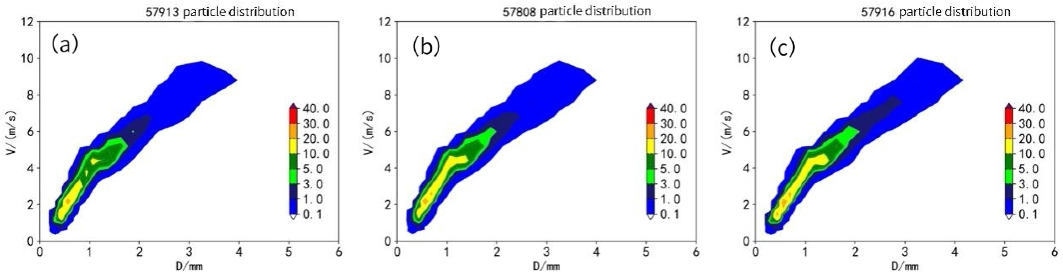
2.1.2. Raindrop Spectrometer and Rain Gauge Data

The raindrop spectrometers used in this paper are all OTT-Parsivel laser raindrop spectrometers, which detect the particle size and particle velocity by measuring the width and time of the laser beam with a wavelength of 650 mm, through the plane of 30 mm wide and 180 mm long. The rain gauge data used are from the tipping bucket rain gauge of the automatic meteorological observation station in Guizhou Province, and the detection accuracy is 0.1 mm. In order to ensure the spatial position coincidence of the raindrop spectrometer and rain gauge, the data from the two instruments used in this paper are from the same meteorological station. The detection time resolutions of the raindrop spectrometer and of the rain gauge are set to 1 min, which ensures the time matching of the two data.Table 1 lists the basic site information.

2.2. Data Quality Control

2.2.1. Data Quality Control of Raindrop Spectrometer

Firstly, the gross error is eliminated. The research shows that raindrop particles more than 6 mm in nature are extremely rare, so this part is destroyed. Subsequently, in order to ensure the stability of the droplet spectrum measurement, the data in which the number of detected raindrops is less than 10 in a single sample are removed as noise. Finally, according to the local D-V relationship, the errors of particle overlap and raindrop spectrometer rain cover splashing particles are eliminated.
ATLA D et al. [18] (1973) found that the final velocity formula of precipitation particles under ideal windless conditions is as follows:
v = 0 , x < 0.03   mm v = 4.323 × x 0.03 v = 9.65 10.3 × e 0.6 x , x > 0.6   mm , 0.03   mm < x 0.6   mm
In the formula, x is the particle diameter, whose unit is mm; v represents the final velocity of the particle, whose unit is m/s.
By counting different types of precipitation samples, the D-V curve of local precipitation particles is fitted, representing the particle size and particle velocity characteristics of regional precipitation. Referring to the data method proposed by Kruger et al. [19] to eliminate the excessive dispersion of velocity sampling, the threshold is set to eliminate the particles in the interval with significant deviation from the reference curve, and the precipitation particles can be retained.

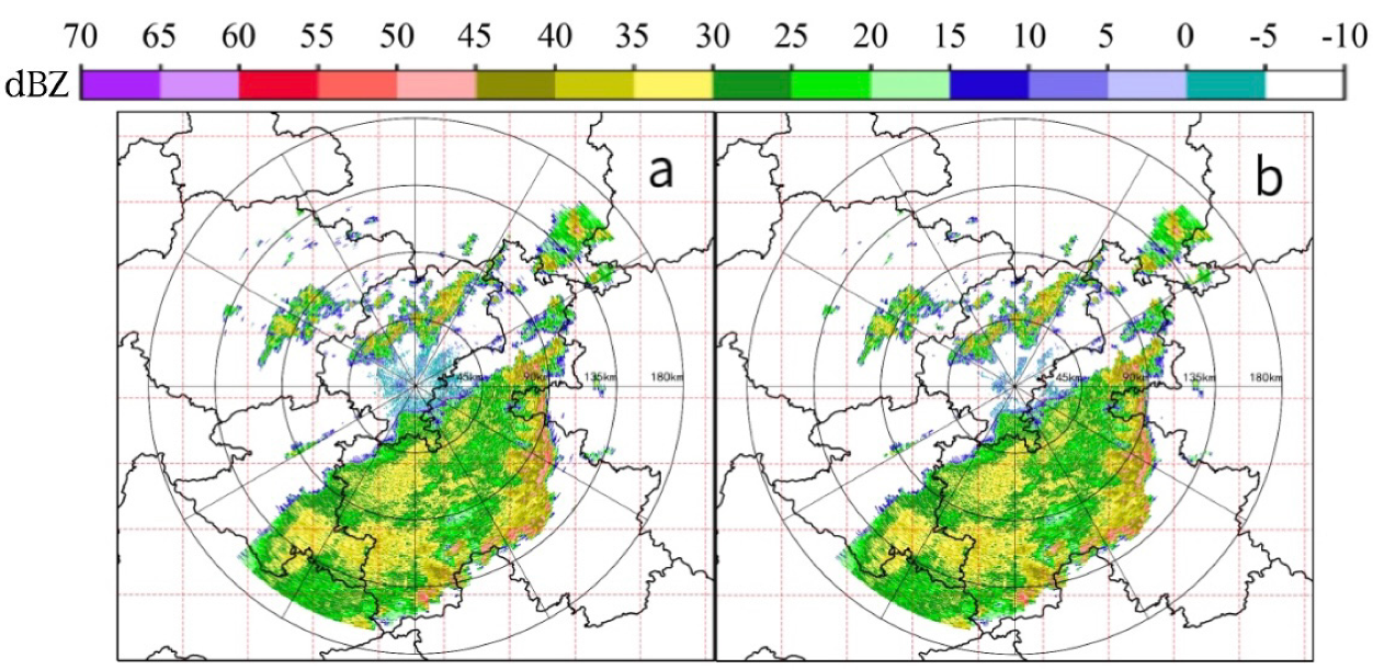
2.2.2. Weather Radar Data Quality Control

Weather radar will detect both meteorological and non-meteorological echoes in the detection process. For some isolated echoes, or thin line-shaped echoes caused by birds, insects, aircraft, etc., speckle filtering can be used to eliminate them. The formula is as follows:
P X = N / N total
In the formula, Ntotal is the total number of distance libraries contained in the 5 × 5 grid centered on the X-th distance library, N is the number of libraries with radar reflectivity values in Ntotal, and Px is the percentage of radar reflectivity in the grid. When Px is less than a certain threshold (default 75% in this paper), the X-distance library calibrated in the radar base data is regarded as the non-meteorological echo being eliminated.
However, it is difficult to eliminate large-scale ground clutter in some areas close to the radar using speckle filtering alone. For this part of the clutter, texture filtering is needed to eliminate it. Firstly, the horizontal texture feature parameter TdBZ is calculated. The horizontal texture feature parameter TdBZ can describe the smoothness of adjacent distance and radial data in the same elevation layer. The formula is as follows:
T d B Z = j = 1 N A i = 1 N B Z i , j Z i , j + 1 2 / N A × N B
In the formula, Zi,j is the radar reflectivity intensity, whose unit is dBZ; i and j are the distance library serial number and the azimuth serial number in the reflectivity library, respectively. NA and NR are the numbers of calculation libraries centered on the calibration distance library in distance and azimuth, respectively.
The vertical texture feature parameter VdBZ can describe the continuity of the echo in the adjacent elevation layers of the same distance library. The VdBZ of the calibrated distance library can be calculated using the following formula:
V d B Z = Z i Z i + 1 / H i + 1 H i
In the formula, Zi and Zi+1 are the radar reflectivity intensity of the upper elevation angle of the calibration range library and the calibration range library, respectively, and their unit is dBZ. Hi and Hi+1 correspond to the elevation angles of the upper layer of the calibration distance bank and the calibration distance bank, respectively.
The horizontal texture features can distinguish stratiform cloud precipitation echo and convective cloud echo, but cannot distinguish precipitation echo and non-precipitation echo. The vertical texture features can distinguish non-precipitation echo and stratiform cloud echo, but cannot distinguish non-precipitation echo and convective cloud echo. Therefore, it is necessary to combine the two. The non-precipitation echo formula is as follows:
V d B Z > 20 dB / km T d B Z > 10 dB 2
It can be seen from Figure 1 that the ground clutter in the area near the radar is effectively suppressed, and some sporadic echoes at the edge of the precipitation echo are also eliminated. After quality control, a complete precipitation echo area can still be obtained.

3. Calculation and Characteristic Analysis of Raindrop Spectrum Parameters

3.1. Calculation of Raindrop Spectrum Parameters

3.1.1. Number Density

The particle number density N(D) represents the total number of raindrop particles per unit volume, and its unit is m−3m−1. The calculation formula is as follows:
N D = i = 1 32 j = 1 32 n i j A × Δ T × V j
In Equation (6), nij represents the number of particles in the i-th particle diameter and the j-th particle velocity; A is the sampling base area of raindrop spectrometer 5400 mm2; ∆T is the sampling time of 60 s; Vj is the sampling particle velocity in m/s.

3.1.2. Precipitation Intensity

The precipitation intensity is the amount of precipitation per unit of time, and the unit is mm/h. The calculation formula was proposed by Pruppacher and Klett [20] as follows:
I = 6 π 10 4 i = 1 32 D i 3 V D i N D i
In Equation (7), Di represents the diameter of the sampled particle, and N(Di) is the number of particles at the current particle diameter and particle velocity.

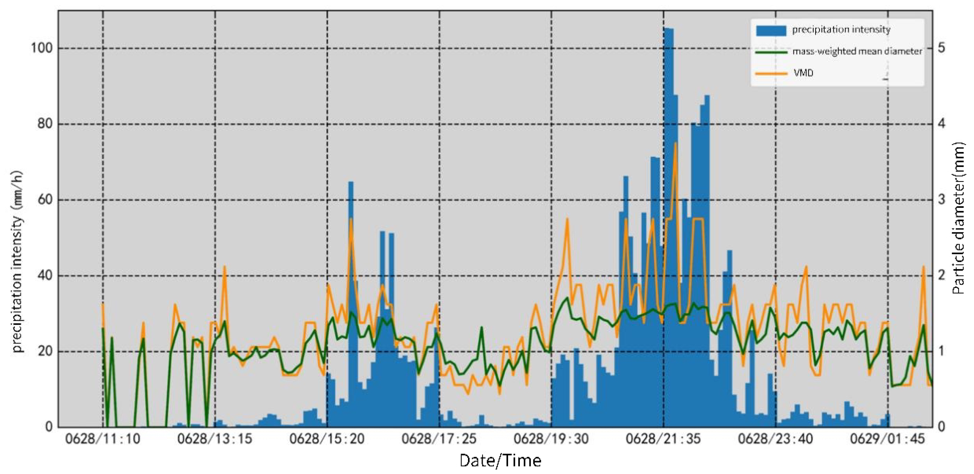
3.1.3. Mean Diameter

The average diameter is the sum of the diameters of all raindrops divided by the total number of raindrops. The formula is as follows:
D l = i = 1 32 N D i D i i = 1 32 N D i

3.1.4. Mass-Weighted Average Diameter

The mass-weighted average diameter is the average diameter of the weighted mass of all particles in the unit volume relative to the total mass of the particles. The unit is mm. The calculation formula is as follows:
D m = i = 1 32 N D i D i 4 i = 1 32 N D i D i 3

3.1.5. VMD

The average volume diameter represents the diameter of the equivalent raindrop whose volume is equal to the average raindrop volume. Its unit is mm. The calculation formula is as follows:
D v = i = 1 32 N D i D i 3 i = 1 32 N D i 1 3

3.1.6. M-P Distribution and GAMMA Distribution

Marshall and Palmer [21] first proposed the M-P distribution. They found that the exponential function can be used to describe the distribution of raindrop size distribution, and established the following formula:
N D = N 0 × exp λ D
In Equation (11), the unit of the particle number density parameter N0 is mm−1m−3, and the unit of the particle size parameter λ is mm−1.
It can be seen from previous studies that the M-P distribution formula is simple and easy to calculate. Still, when describing the small-particle-size and large-particle-size regions, there is an inevitable error between the actual observation data. To illustrate the raindrop size distribution more accurately, Ulbrich [22] proposed a method based on the M-P distribution to regard the raindrop size distribution as the GAMMA distribution. This method can correct the distribution pattern in the regions with small particle size or large particle size. At this time, the raindrop spectrum description function changes from the original two-parameter exponential function to the three-parameter function form. The formula is as follows:
N D = N 0 × D μ × exp λ D
The shape factor u in Equation (12) is a dimensionless parameter. When μ > 0, the function curve bends upward. When μ < 0, the function curve bends downward. When μ = 0, the formula becomes an M-P distribution.

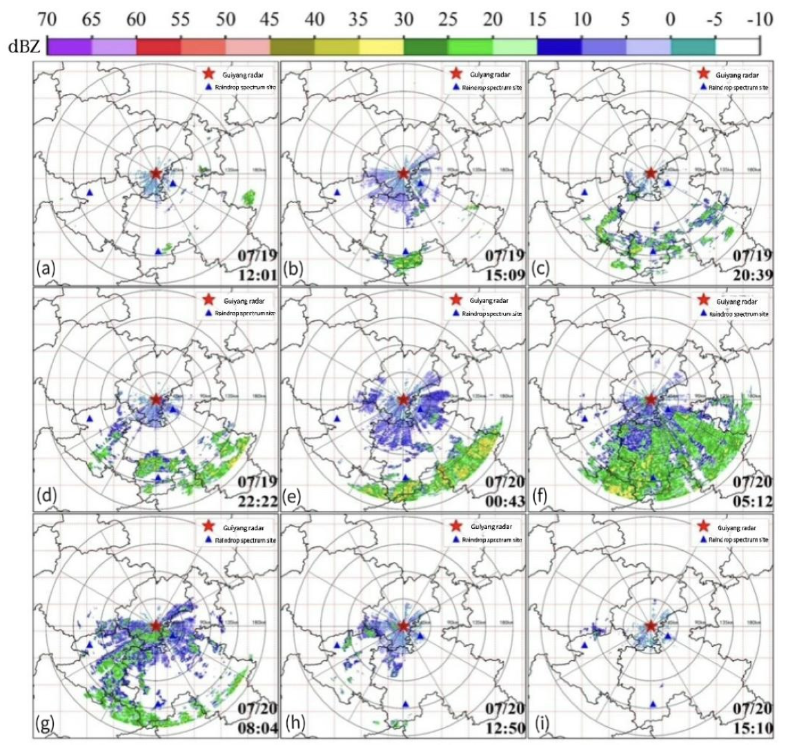
3.2. Analysis of Raindrop Spectrum Characteristics

In Figure 2, the horizontal axis is the particle diameter, the vertical axis represents the final velocity of the particle, and different particle number densities are distinguished by color. It can be seen from the average distribution of particles from March to August 2020 in the figure that the corresponding particle size terminal velocities and particle distribution patterns of the three stations are similar, and they are concentrated in the small-particle-size area. The difference is that the particle concentration from the Longli (57913) station, in the range of 1–1.5 mm, is more dispersed than those of the other two stations, and the spectrum width of the Luodian (57916) station is wider than those of the other two stations.
Figure 3 shows the particle number density distribution corresponding to each particle size in the average raindrop spectrum. The horizontal axis represents the particle size, and the vertical axis represents the particle number density. The fitting coefficients of the three-site M-P distribution and the GAMMA distribution are shown in Table 2.
The correlation coefficient parameters in Table 2 and Table 3 show that the GAMMA distribution’s fitting effect is significantly more potent than that of the M-P distribution. The three-parameter GAMMA distribution is more flexible than the two-parameter M-P distribution, which can depict more curve details. At the same time, the natural raindrop spectrum of the three stations is unimodal, resulting in a significant error between the M-P distribution and the actual value in the small-particle-size area. When the GAMMA distribution fits the unimodal particle spectrum, the steeper the curve on both sides of the peak, the larger the μ and λ values needed. Still, this would cause a great N0 value to reduce the error between the peak value of the fitting curve and the actual value. It would also lead to underestimation in the large-particle-size (D > 1 mm) area, where the slope of the actual value curve is relatively moderate, and the M-P distribution in the large particle-size-area performs better.
The average diameter, mass-weighted average diameter, and average volume diameter are used as parameters that can reflect the characteristics of the particle spectrum. Finding the parameters with the highest consistency with rainfall intensity lays the foundation for estimating precipitation later. The correlation coefficient between each diameter and rainfall intensity is shown in Table 4.
The data used in Table 4 are the precipitation data of three stations, taken from March to August 2020. To ensure the quality of the sample, the samples with rainfall intensity of less than 1 mm/h are eliminated. The data in the table show that the correlation coefficient between the average diameter and rainfall intensity is the lowest, and the correlation between the average volume diameter and rainfall intensity is the highest. Figure 4 selects a heavy precipitation process in order to find the area where the mass-weighted average diameter and the average volume diameter differ.
Figure 4 shows a heavy precipitation process on 28 June. The horizontal axis represents the precipitation process time, the left axis represents the precipitation intensity, and the right axis represents the particle diameter of the mass-weighted average diameter and the average volume diameter. The precipitation intensity value of this process shows a bimodal distribution. It can be seen that, when the precipitation intensity is not high early, late, and between the two peaks of precipitation, the curves of the mass-weighted average diameter and average volume diameter almost coincide, which are in good agreement with the precipitation intensity value. However, the performance of the average volume diameter in the heavy precipitationarea is better than that of the mass-weighted average diameter. The correlation coefficients between the mass-weighted average diameter and average volume diameter, and the precipitation intensity were 54.84% and 69.15%, respectively.

4. Precipitation Estimation Method and Result Analysis

4.1. Precipitation Estimation Method

4.1.1. Dynamic Z-I Relationships

The dynamic Z-I relationship method is based on the Z = aIb index relationship, and the fast real-time updated radar-automatic rainfall station data adjust the a and b coefficients in the relationship. Different Z-I relationships can be used to estimate precipitation with the change in the precipitation process. This method uses the weather radar detection data and the automatic rainfall station data from the previous hour to calculate the optimal parameters of the current Z-I relationship. It uses this relationship to estimate the recent precipitation. Firstly, the value range of the a and b coefficients is determined. Wang et al. [23] pointed out in their study that the value range of a is 16–1200, and that of b is 1–2.87. In order to save calculation time, when calculating the optimal coefficient, 60 a values are taken, from 16 to 1200 with an interval of 20, and 38 b values are taken, from 1 to 2.87 with an interval of 0.05, to calculate 60 × 38 groups of Z = amIbn (m = 1, 2,……., 59, 60; n = 1, 2,….., 37, 38), and simultaneously calculate 60 × 38 discriminant functions, CTF2 (Zhang Peichang et al. [24]), as follows.
C T F 2 = min H i G i 2 + H i G i
In Equation (13), Hi is the inversion precipitation of the Z-I relationship, Gi is the precipitation measured at the automatic rainfall station, and i is the sequence of the automatic rainfall station. The Z-I relationship with the lowest CTF2 value is the optimal one to apply to radar echo estimation precipitation.

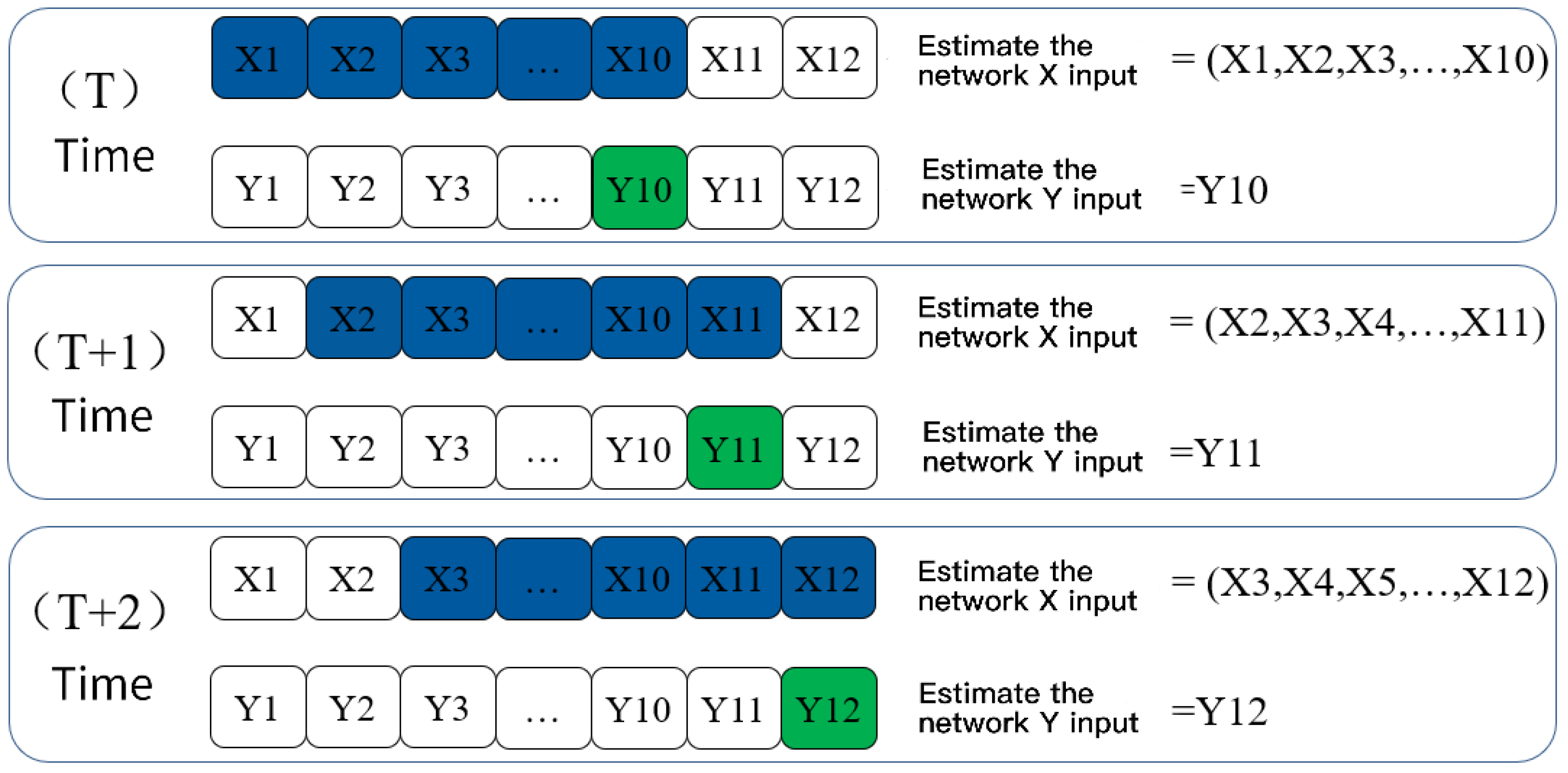
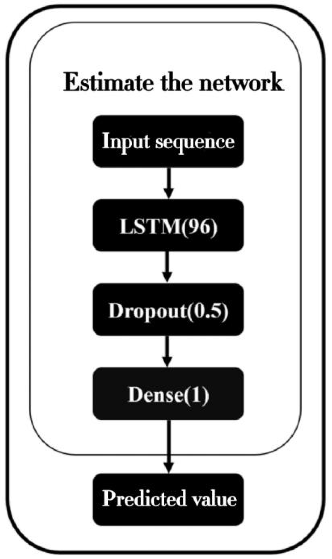
4.1.2. Neural Network Method

Considering the temporal characteristics of precipitation, this paper uses the LSTM neural network to build and train the model. In terms of data, Guiyang weather radar data, raindrop spectrometer, and the automatic rain gauge data from Longli (57913), Puding (57808), and Luodian (57916) automatic weather stations were used. The data overview is shown in Table 5.
The construction of the data set is significant for using the neural network to estimate precipitation. The closer the relationship between the input eigenvalues and the calibration values to be output, the more accurate the final training results. The calibration value to be estimated in this paper is precipitation. Therefore, the reflectivity data in the weather radar, as well as the particle diameter, particle falling speed, and particle number density parameters in the inversion formula of the raindrop spectrum precipitation intensity were selected as the input eigenvalues of the neural network. Considering the distance between the raindrop spectrum station and the radar station, and drawing on experience in the process of model debugging, select 1–3 lamination scan data as feature value input, as shown in Table 6.
When establishing the neural network input data set, the time sliding construction is used to enrich the data set, and the input diagram of the estimated data set is shown in Figure 5.
As shown in Figure 5, the X input of the estimation network keeps the ten sample sizes unchanged and slides on the time axis in turn. The Y input maintains the time corresponding to the last sample of the X input—that is, using the data from the previous hour to estimate the current time’s precipitation.
The basic structure of the neural network is shown in Figure 6.
The data are first entered into the LSTM layer for temporal feature extraction, and then the dropout layer is used to increase the network’s generalization ability. Finally, the predicted value is output in the BP layer of a single neuron.
In this paper, according to the method of dividing convective clouds and stratiform clouds proposed by Tokay et al. [25], two representative precipitation processes and 45-day cumulative precipitation were selected to estimate rainfall using the dynamic Z-I method and neural network method, respectively. The data were used to compare the effects of the Longli (57913), Puding (57808), and Luodian (57916) automatic weather stations. The station information is shown in the table.
In terms of the estimation accuracy evaluation index, correlation coefficient (Cor), mean relative error (MRE), mean absolute error (MAE), and root mean square error (RMSE) are used. The calculation formula is as follows:
C o r = i = 1 n R e s t i R e s t ¯ R r e a l i R r e a l ¯ i = 1 n R e s t i R e s t ¯ 2 R r e a l i R r e a l ¯ 2
M R E = 1 n i = 1 n R e s t i R r e a l i R r e a l i × 100 0 0
M A E = 1 n i = 1 n R e s t i R r e a l i
R M S E = 1 n i = 1 n R e s t i R r e a l i 2
The correlation coefficient can compare the linear correlation between the two sequences. The higher the correlation is, the closer the correlation coefficient is to 1. The average absolute error is the average value of the fundamental error, which can reflect the positive and negative offset parts of the error. The average relative error is the average value of the absolute error percentage to the actual value, representing the measurement results’ reliability. The root means the square error is the square root of the mean fair sum of the deviation between the observed value and the actual value, and is used to measure the divergence between the observed value and the actual value. It is more sensitive to singular values.

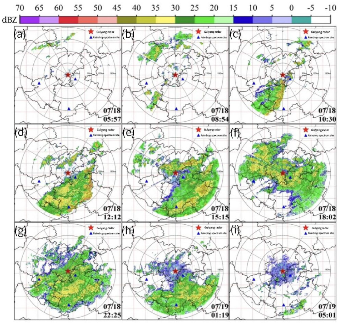
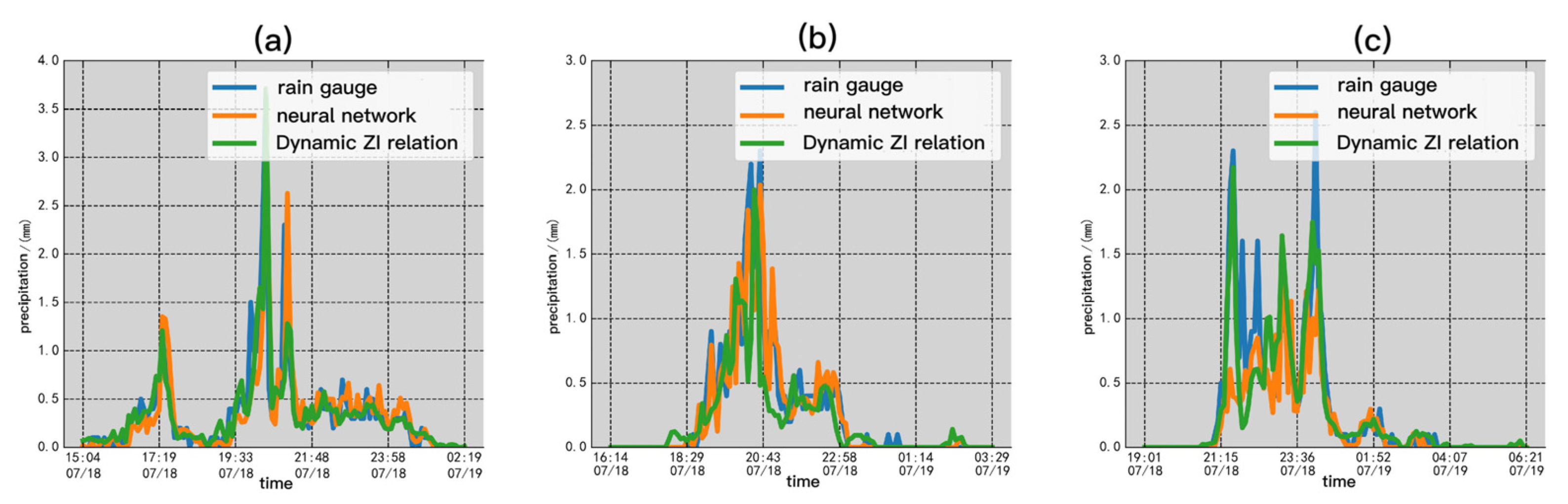
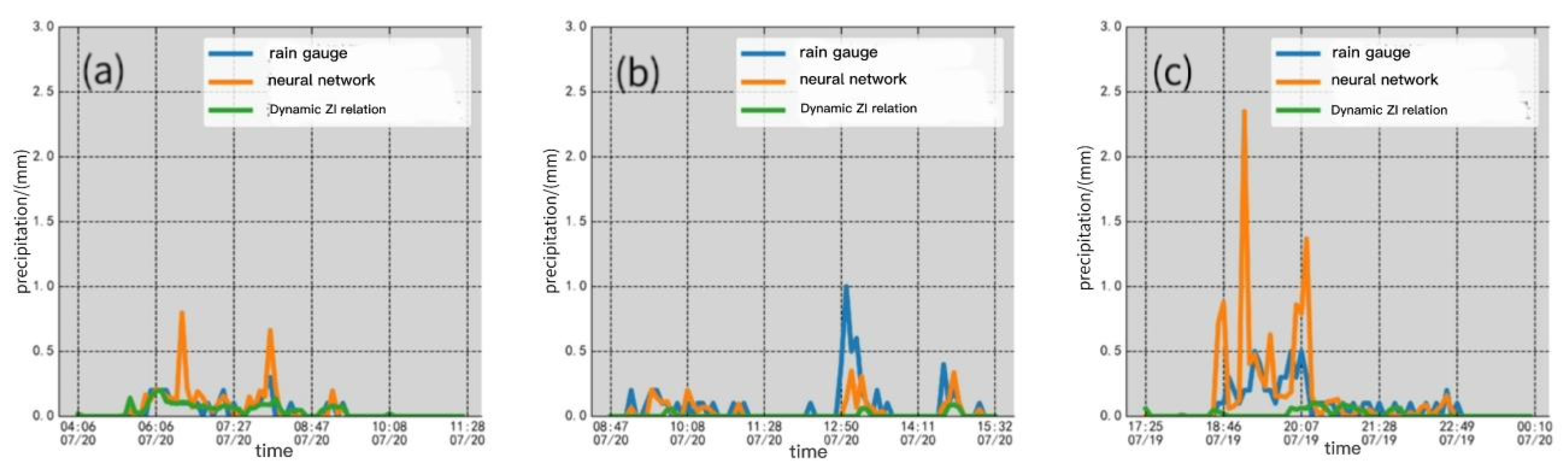
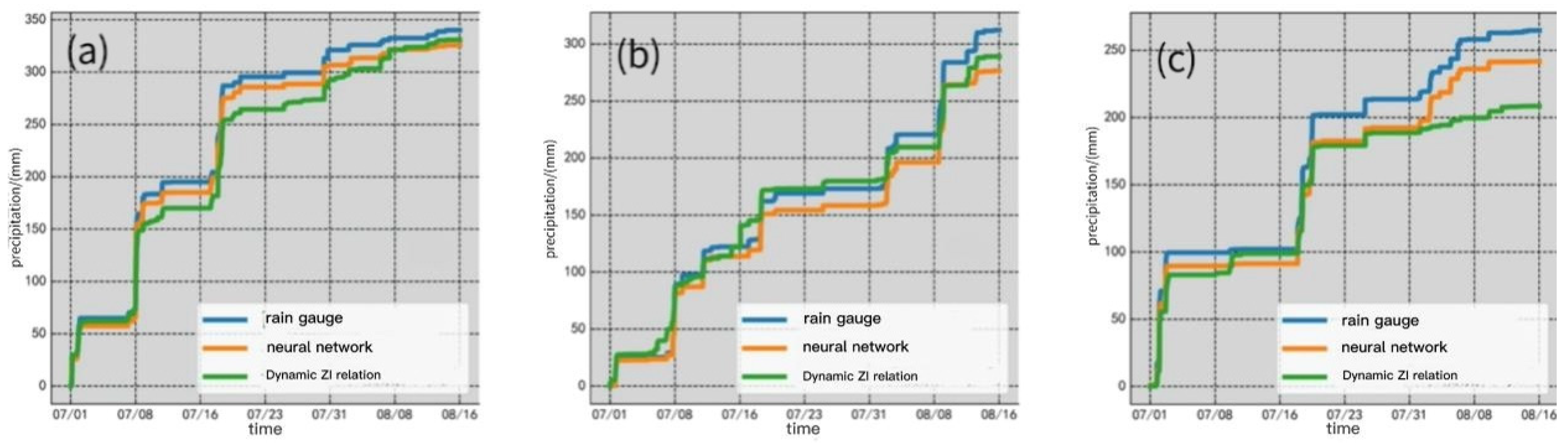
4.2. Analysis of Precipitation Estimation Results

Firstly, a convective cloud precipitation process occurring on 18 July 2020 was selected for analysis. The weather development process is as follows.
As shown in Figure 7, at 5:57 on 18 July 2020, an unmistakable echo appeared near the junction of Bijie, Zunyi, and Luzhou in Sichuan Province, in the northwest direction from Guiyang. The maximum combined reflectivity reached 53.2 dBZ, and the echo continued to develop and move southeastward. At about 8:00 BST, a strong echo band appeared over the junction of southwest Anshun and southwest Guizhou in the southwest of Guiyang, and quickly moved to the northeast. From Figure 7d, it can be seen that the echo gradually evolved into a northeast–southwest squall line echo. At this time, the lower atmosphere in southern Guizhou showed a strong wind field convergence phenomenon. At 14:00, with the continuous development of the weather phenomenon, the squall line the squall line gradually gradually weakens and tends to die, but the rear part of the squall line still maintains a high reflectivity intensity. The echo area covered most of southern Guizhou, and the two independent echoes were connected and began to merge, affecting the region. At 18:00, the echo over the Qiannan area dissipated, but the precipitation cloud was continuously transported from the solid southeast wind to the Qiannan area. Within a few hours, the echo area slowly moved southward, the precipitation echo was evenly distributed, and the intensity remained unchanged with short-term strong wind. Until 5 o’clock on 19 July 2020, the precipitation area continued to dissipate.
The convective cloud precipitation estimated with the neural network method and dynamic Z-I relationship method is shown in Figure 8.
The real-time estimation of the rainfall evaluation index is shown in Table 7.
From the fitting curve in Figure 8 and the data in Table 7, it can be seen that the neural network method outperforms the dynamic Z-I relationship method at all three stations in terms of real-time correlation coefficients. For MRE, MAE, and RMSE, the error of the neural network method in the Longli (57913) and Puding (57808) stations is smaller than that of the dynamic Z-I relationship method, and slightly higher than that of the dynamic Z-I relationship method at Luodian (57916) station. Dynamic Z-I relationship: The Z-I relationship is corrected using the first ten body sweep data and raingauge data. When the automatic rain gauge does not detect precipitation information, the Z-I relationship is set Z = 16 × I1.0. Only a tiny intensity of radar reflectivity can invert a certain precipitation intensity. The advantage of this setting is that it can make up for the residual error from the tipping bucket of the automatic rain gauge to a certain extent. Still, it is limited to the quality of the radar data and the automatic rain gauge data. If the radar detection echo is shorter before the precipitation data, it will prevent the precipitation from being overestimated. The neural network method is less effective at estimating the precipitation start period, and there is a specific lag phenomenon. This is because the neural network needs to learn from rich samples in order to establish the model, including precipitation samples, non-precipitation samples, and some samples with mismatched precipitation information. Therefore, for the neural network to determine the precipitation start time, the input sample needs to contain a sufficient amount of precipitation samples, so it will affect the determination of the precipitation start time. When the precipitation intensity in the latter part of the precipitation is large and the precipitation is continuous, the actual precipitation can be accurately reflected regardless of the neural network or the dynamic Z-I relationship. The dynamic Z-I relationship and the neural network method can accurately describe the convective cloud precipitation process, independent of the distance from the station to the radar.
Secondly, a continuous stratiform cloud precipitation process on 19 July 2020 was selected for analysis. The weather process is as follows.
As shown in Figure 9, at 12:00 on 19 July, scattered echoes appeared and developed slowly over the junction of southern Guizhou, Guangxi, and Yunnan. During this period, the wind force in Guizhou was low, and the wind field was relatively stable. At 17:00, the echo development gradually covered the target site. At this time, under the influence of slight southeast wind, the echo development accelerated but remained stable, and the space did not change much. The echo gradually attenuated and dissipated by 0:00 on 20 July. Then, a slight southerly wind carried a large area of echoes and continued to affect the southern part of Guizhou until the end of the weather process at 13:00 on 20 July. From the radar echo map, the weather phenomenon has low precipitation intensity and a simple process. The echo is not seen in the second and third layers of the radar volume scan, it indicating that the development of precipitation clouds is thin, and the wind direction and wind speed are relatively stable during the entire duration of precipitation, and there is no apparent convergence phenomenon.
The convective cloud precipitation estimated with the neural network method and dynamic Z-I relationship method is shown in Figure 10.
Table 8 shows the real-time rainfall estimation evaluation indicators.
It can be seen from the data shown in Table 8 that, except for the similar results obtained using the two methods at Longli (57913) station, which is close to the radar station, the neural network method is far better than the dynamic Z-I method in the precipitation estimation of the other two stations. Still, the overall estimation effect is far less than the convective cloud process estimation. Figure 10b,c show that the dynamic Z-I relationship method does not invert precipitation on the time series estimated at the Puding (57808) and Luodian (57916) stations. From the weather background, it can be seen that the precipitation process is weak, and the clouds are thin. Examining the radar base data, it is found that the two stations far from the radar station can detect very little echo information, which directly affects the estimation effect of the dynamic Z-I relationship. The neural network method uses multi-source data from radar and a raindrop spectrometer for estimation. Compared with the single-source data, the dependence is reduced, and the estimation effect is improved compared with the dynamic Z-I relationship method. However, due to the lack of precipitation information detected during the stratiform cloud precipitation process and the frequent interruption of precipitation, the estimation effect still needs to be significantly different from that of convective cloud precipitation.
Finally, the neural network and the dynamic Z-I methods were used to estimate the total precipitation of the three stations for 45 days from 1 July 2020, to 16 August 2020, respectively. Calculating cumulative rainfall in an area can reflect the applicability of the estimation method and the universality of different types of precipitation. The cumulative precipitation of rain gauges at the Longli (57913), Puding (57808), and Luodian (57916) stations during the selected period were 340.0 mm, 312.0 mm, and 264.6 mm, respectively. The results are shown in Figure 11.
Table 9 lists the estimated cumulative rainfall evaluation indexes of the three stations.
From the precipitation measured with the rain gauge, the rainfall estimated using the neural network, and the precipitation estimated using the dynamic Z-I relationship shown in Figure 11, along with the comprehensive evaluation index, it can be seen that the rainfall estimates made using the dynamic Z-I relationship method and the neural network method have a firm consistency with the measured rainfall. Still, the dynamic Z-I relationship is reflected in some weak precipitation processes, but the dynamic Z-I relationship did not reflect satisfactory effects in some weak precipitation processes, such as Puding (57808); the dynamic Z-I relationship of multiple inefficient precipitation processes after August in Luodian (57916) station also shows apparent underestimation, and a weak precipitation process on July 10 was overestimated. By examining the base data and radar echo map on 10 July, it is found that the radar detected a strong echo lasting about one hour before the automatic rainfall station detected the precipitation. Because the dynamic Z-I relationship was Z = 16 × I10 when the rainfall data of the rainfall station is 0, the strong echo in the period of 0 times the rainfall station data caused the weak precipitation process to be overestimated. The relative errors of Longli (57913), Puding (57808) and Luodian (57916) stations using dynamic Z-I relationships to estimate cumulative precipitation were −2.68%, −7.41% and −21.23%, respectively, and the relative errors estimated by neural networks were −4.25%, −11.35% and −8.68%. With regards to the cumulative precipitation of the Longli and Puding stations, the final relative error of the neural network is slightly worse than that of the dynamic Z-I relationship. Still, the neural network is better than the dynamic Z-I relationship in terms of the correlation coefficient index. Combined with Figure 11a, it can be found that the dynamic Z-I relationship shows a certain underestimation in several heavy precipitation processes. Still, it shows apparent overestimation in several weak precipitation processes in August, and finally offers a small cumulative error and low correlation coefficient. From Figure 11c, it can be obtained that dynamic Z-I is affected by the quality of radar detection data, and the estimation effect of stratomorph cloud precipitation is poor at a distance from the radar station, which is directly reflected in the cumulative precipitation error of −21.23% at Luodian (57916) station.

5. Conclusions

In this paper, the characteristics of the raindrop spectra of Longli (57913), Puding (57808), and Luodian (57916) stations in Guizhou Province were analyzed to find the diameter parameters with a strong correlation with rainfall intensity. Thereafter, the multi-source data from weather radar, raindrop spectrometer, and surface rain gauge in Guiyang, Guizhou Province, were used to estimate precipitation. The conclusions are as follows:
(1) After analyzing the raindrop spectral distribution at Longli, Puding, and Luodian stations, it was found that the peak value and spectral width of particle distribution at Luodian (57916) station were different from those of the other two stations, indicating that the raindrop spectral distribution was further between different regions. The correlation coefficients of the three sites, as fitted using the M-P distribution, were 83.52%, 85.25%, and 81.69%, respectively. The correlation coefficients provided using the GAMMA distribution were 95.65%, 95.84%, and 94.82%, indicating that the fitting effect of the GAMMA distribution was better. The correlation coefficients between the mass-weighted average diameter of the three stations and the rainfall intensity were 46.89%, 49.51%, and 47.03%, respectively, slightly lower than the 67.80%, 71.28%, and 71.46% of the mass-weighted average diameter. Using a heavy rainfall example, it was found that the two diameters had the same fitting effect on the rainfall intensity at low rainfall intensity. Still, the average volume diameter was more sensitive at heavy rainfall intensity.
(2) Based on the three-source data from the Guiyang weather radar, Parsivel raindrop spectrometer, and automatic rain gauge, the neural network and dynamic Z-I relationship methods were used to estimate the precipitation. In the process of convective cloud precipitation, the correlation coefficients of the neural network method and the dynamic Z-I relationship method at the three stations were 0.8745, 0.9125, and 0.8676 and 0.8432, 0.7763, and 0.8658, respectively. This shows that the dynamic Z-I relationship and the LSTM neural network method are both consistent with the measured rainfall of the automatic rain gauge.
(3) In stratiform cloud precipitation, the correlation coefficients of the neural network and dynamic Z-I relationship methods at the three stations were 0.7114, 0.4984, and 0.4902 and 0.6933, 0.0902, and 0.1409, respectively. The dynamic Z-I relationship method is greatly affected by weather radar detection data. At stations where the echo development is thin and far away from the weather radar, the weather radar cannot stably provide high-quality detection data. Currently, the neural network method using multi-source data has more advantages.
(4) Based on the three-source data from the Guiyang weather radar, Parsivel raindrop spectrometer, and automatic rain gauge, the neural network method and the dynamic Z-I relationship method were used to estimate the total precipitation of the three stations for 45 days. In the comparison of cumulative estimated rainfall, it was found that there is a strong consistency between the dynamic Z-I relationship method and the neural network method to estimate precipitation and the measured precipitation. The relative errors of the three sites using neural network estimation were −4.25%, −11.35%, and −8.68%, respectively. The relative errors of the cumulative precipitation estimated using the dynamic Z-I relationship were −2.68%, −7.41%, and −21.23%, respectively. The final comparable mistake of the neural network in the cumulative precipitation of the Longli and Puding stations was slightly worse than that of the dynamic Z-I relationship. Still, the correlation coefficient between the precipitation estimated using the neural network and the real value remained higher than that of the dynamic Z-I relationship.

Author Contributions

Conceptualization, F.W., Y.C., Q.W., T.Z. and D.S.; methodology, T.Z.; writing—original draft preparation, F.W., Y.C. and Q.W.; writing—review and editing, F.W.; supervision, D.S.; funding acquisition, F.W. All authors have read and agreed to the published version of the manuscript.

Funding

This work was supported by the Sichuan Provincial Natural Science Foundation (2022NSFSC0208) and the Open Fund Project of the Key Laboratory of Land Surface Processes and Climate Change in Cold and Arid Regions, Chinese Academy of Sciences (LPCC2020009).

Institutional Review Board Statement

Not applicable for studies not involving humans or animals.

Informed Consent Statement

Not applicable for studies not involving humans.

Data Availability Statement

The data used to support the findings of this study are available from the corresponding author upon request.

Conflicts of Interest

The authors declare no conflict of interest.

References

  1. Huang, Z.W.; Peng, S.Y.; Zhang, H.R.; Zheng, J.F.; Zeng, Z.M.; Wang, Y.Y. Characteristics of raindrop size distribution in Anxi, Fujian. J. Appl. Meteorol. Sci. 2022, 33, 205–217. [Google Scholar]
  2. Chakravarty, K.; Raj, P.E. Raindrop size distributions and their association with characteristics of clouds and precipitation during monsoon and post-monsoon periods over a tropical Indian station. Atmos. Res. 2013, 124, 181–189. [Google Scholar] [CrossRef]
  3. Zhao, C.C.; Zhang, L.J.; Liang, H.H.; Li, L.; Liu, Y.L. Analysis of summer raindrop spectrum characteristics in Beijing mountainous and plain areas. Meteorol. Mon. 2021, 47, 830–842. [Google Scholar]
  4. Zhang, Y.X.; Han, H.B.; Guo, S.Y.; Tian, J.B.; Tang, W.T. Characteristics of raindrop size distribution and Z-R relationship of different precipitation clouds in summer at the southern foot of Qilian Mountains. Arid Zone Res. 2021, 38, 1048–1057. [Google Scholar]
  5. Chen, S. Research on Precipitation Phenomenon Recognition Technology Based on Raindrop Spectrum and Machine Learning; Nanjing University of Information Science and Technology: Nanjing, China, 2021. [Google Scholar]
  6. Jing, G.F.; Luo, L.; Guo, J.; Cui, X.L. Application of raindrop spectrometer in weather radar precipitation estimation. Foreign Electron. Meas. Technol. 2020, 39, 11–18. [Google Scholar] [CrossRef]
  7. Liu, S.N.; Wang, G.L. The influence of DSD parameters on precipitation estimation by dual-frequency radar. Plateau Meteorol. 2020, 39, 570–580. [Google Scholar]
  8. Zhang, Y.; Liu, L.P.; He, J.X.; Wen, H. Application of raindrop spectrometer network data in radar quantitative precipitation estimation. Torrential Rain Disasters 2016, 35, 173–181. [Google Scholar]
  9. Zhou, L.M.; Zhang, H.S.; Wang, J.; Wang, Q.; Chen, X.L. Characteristics of raindrop spectrum of a typical stratocumulus mixed cloud precipitation process. Meteorol. Sci. Technol. 2010, 22, 73–77. [Google Scholar]
  10. Peng, Y.Z.; Wang, Q.; Yuan, C.A.; Lin, K.P. Application of data mining technology in meteorological forecast research. J. Drought Meteorol. 2015, 33, 19–27. [Google Scholar]
  11. Kang, J.L.; Wang, H.M.; Yuan, F.F.; Wang, Z.P.; Huang, J.; Qiu, T. Prediction of Precipitation Basedon Recurrent Neural Networks in Jingdezhen, Jiangxi Province, China. Atmosphere 2020, 11, 246. [Google Scholar] [CrossRef] [Green Version]
  12. Shen, H.J.; Luo, Y.; Zhao, Z.C.; Wang, H.J. Research on summer precipitation prediction in China based on LSTM network. Clim. Chang. Res. 2020, 16, 263–275. [Google Scholar]
  13. Tang, W.; Ma, S.C.; Chen, R. The early warning method of rainfall-induced debris flow in northwestern Sichuan based on LSTM. J. Guilin Univ. Technol. 2020, 40, 719–725. [Google Scholar]
  14. Liu, X.; Zhao, N.; Guo, J.Y.; Guo, B. Prediction of monthly precipitation over the Tibetan Plateau based on LSTM neural network. J. Earth Inf. Sci. 2020, 22, 1617–1629. [Google Scholar]
  15. Chen, H.; Qi, Z.F. Monthly precipitation prediction in eastern Sichuan based on LSTM network. Water Resouces Power 2021, 39, 14–17+13. [Google Scholar]
  16. Yashon, O.O.; Rodrick, C.; Alice, N.W. Rainfall and Runoff Time-Series Trend Analysis Using LSTM Recurrent Neural Network and Wavelet Neural Network with Satellite-Based Meteorological Data: Case Study of Nzoia Hydrologic Basin. Complex Intell. Syst. 2021, 8, 213–236. [Google Scholar]
  17. Yang, Q.; Qin, L.; Gao, P.; Zhang, R.B. Based on the EEMD-LSTM model, the annual precipitation prediction of the economic belt on the northern slope of the Tianshan Mountains. Arid Zone Res. 2021, 38, 1235–1243. [Google Scholar]
  18. Atlas, D.; Srivastava, R.C.; Sekhon, R.S. Doppler characteristics of precipitation at vertical incidence. Rev. Geophys. Space Phys. 1973, 11, 1–35. [Google Scholar] [CrossRef]
  19. Kruger, A.; Krajewski, W.F. Two-dimensional video disdrometer: A description. J. Atmos. Ocean. Technol. 2002, 19, 602–617. [Google Scholar] [CrossRef]
  20. Pruppacher, H.R.; Klett, J.D.; Wang, P.K. Microphysics of Clouds and Precipitation; Springer: Berlin/Heidelberg, Germany, 1998. [Google Scholar]
  21. Marshall, J.S.; Palmer, W.M. The distribution of raindrops with size. J. Atmos. Sci. 1948, 5, 165–166. [Google Scholar] [CrossRef]
  22. Ulbrich, C.W. Natural variations in the analytical form of the raindrop size distribution. J. Clim. Appl. Meteorol. 1983, 22, 1764–1775. [Google Scholar] [CrossRef]
  23. Wang, Y.; Feng, Y.R.; Cai, J.H.; Hu, S. Z-I relationship estimation method of radar quantitative precipitation dynamic classification. J. Trop. Meteorol. 2011, 27, 601–608. [Google Scholar]
  24. Zhang, P.C.; Du, B.Y.; Dai, T.P. Radar Meteorology; Meteorological Press: Beijing, China, 2001; pp. 181–187. [Google Scholar]
  25. Tokay, A.; Petersen, W.A.; Gatlin, P.; Matthew, W. Comparison of Raindrop Size Distribution Measurements by Collocated Disdrometers. J. Atmos. Ocean. Technol. 2013, 30, 1672–1690. [Google Scholar] [CrossRef]
Figure 1. Quality control effect diagram of weather radar base data (a) before quality control and (b) after quality control.
Atmosphere 14 01031 g001
Figure 2. Particle distribution map: (a) Longli (57913) station, (b) Puding (57808) station, and (c) Luodian (57916) station.
Atmosphere 14 01031 g002
Figure 3. Average raindrop size distribution, M-P distribution, and GAMMA distribution fitting: (a) Longli (57913) station, (b) Puding (57808) station, and (c) Luodian (57916) station.
Atmosphere 14 01031 g003
Figure 4. Changes in mass-weighted average diameter and average volume diameter with precipitation intensity.
Atmosphere 14 01031 g004
Figure 5. Estimate network and benchmark network input diagram.
Atmosphere 14 01031 g005
Figure 6. The basic structure diagram of the estimated neural network.
Atmosphere 14 01031 g006
Figure 7. Radar echo of precipitation process on 18 July 2020: (a) 07/18 05:57, (b) 07/18 08:54, (c) 07/18 10:30, (d) 07/18 12:12, (e) 07/18 15:15, (f) 07/18 18:02, (g) 07/18 22:25, (h) 07/19 01:19, and (i) 07/19 05:01.
Atmosphere 14 01031 g007
Figure 8. Rainfall estimation of convective cloud precipitation process: (a) Longli (57913) station, (b) Puding (57808) station, and (c) Luodian (57916) station.
Atmosphere 14 01031 g008
Figure 9. Radar echo of precipitation process on 19 July 2020: (a) 07/19 12:01, (b) 07/19 15:09, (c) 07/19 20:39, (d) 07/19 22:22, (e) 07/20 00:43, (f) 07/20 05:12, (g) 07/20 08:04, (h) 07/20 12:50, (i) 07/19 15:10.
Atmosphere 14 01031 g009
Figure 10. Estimated precipitation of stratiform cloud precipitation process: (a) Longli (57913) station, (b) Puding (57808) station, and (c) Luodian (57916) station.
Atmosphere 14 01031 g010
Figure 11. Comparison of estimated cumulative rainfall: (a) Longli (57913) station, (b) Puding (57808) station, and (c) Luodian (57916) station.
Atmosphere 14 01031 g011
Table 1. Basic information of raindrop spectrum stations.
Station NumberStation NameGeographical CoordinatesDistance from Radar
57913Longli106.98° E, 26.45° N30.21 km
57808Puding105.74° E, 26.31° N99.95 km
57916Luodian106.76° E, 25.43° N129.03 km
Table 2. Mean raindrop spectrum M-P distribution fitting parameters.
Station Name Station NumberN0λCorrelation Coefficient
Longli (57913)85.5219−1.150783.52%
Puding (57808)84.5301−1.024385.25%
Luodian (57916)69.1213−0.915881.69%
Table 3. GAMMA distribution fitting parameters of average raindrop size distribution.
Station Name Station NumberN0µλCorrelation Coefficient
Longli(57913)1,177,999.136.020911.109295.65%
Puding(57808)154,920.625.16948.630195.84%
Luodian(57916)62,872.314.30277.739694.82%
Table 4. Correlation coefficients between diameter and rainfall intensity.
Station Name Station NumberCorrelation Coefficient between Average Diameter and Rainfall IntensityCorrelation Coefficient between Mass Weighted Average Diameter and Rainfall IntensityCorrelation Coefficient between Average Volume Diameter and Rainfall Intensity
Longli (57913)25.04%46.89%67.80%
Puding (57808)28.45%49.51%71.28%
Luodian (57916)18.13%47.03%71.46%
Table 5. Data Overview.
DataStateStart TimeDeadlineSample Size
Raindrop spectrometer,
weather radar,
automatic rain gauge
train15 April 2019 0:00
3 March 2020 0:04
17 July 2019 23:58
30 June 2020 23:57
49,297
inspection1 July 2020 0:0316 August 2020 06:0512,126
Table 6. Estimated neural network input overview.
EigenvalueEstimated Value
Radar reflectivity intensity (1–3 layers)A rain gauge measures precipitation
Inversion of particle number density with raindrop spectrometer
Average particle velocity inversion with raindrop spectrometer
Raindrop spectrometer inversion average volume diameter
Table 7. Evaluation index of rainfall estimation in convective cloud precipitation process.
SiteEstimating MethodReal-Time Correlation CoefficientMREMAERMSE
Longli (57913)Dynamic Z-I0.84320.50460.14620.2745
Neural network0.87450.46460.12280.2454
Puding (57808)Dynamic Z-I0.77630.80390.13240.2962
Neural network0.91250.76280.09350.1884
Luodian (57916)Dynamic Z-I0.86580.77990.13570.3379
Neural network0.86760.79860.13720.3412
Table 8. Rainfall estimation and evaluation index of the stratiform cloud precipitation process.
SiteEstimating MethodReal-Time Correlation CoefficientMREMAERMSE
Longli (57913)Dynamic Z-I0.69330.80680.02670.0479
Neural network0.71140.80080.04010.1047
Puding (57808)Dynamic Z-I0.09020.97940.07040.1721
Neural network0.49840.87710.05640.1416
Luodian (57916)Dynamic Z-I0.14090.93960.08800.1445
Neural network0.49020.84090.11830.3211
Table 9. Estimated cumulative rainfall evaluation index.
SiteEstimating MethodCorrelation CoefficientMREMAERMSERelative Error
Longli (57913)Dynamic Z-I0.99510.081619.421122.0374−2.68%
Neural network0.99980.052610.315610.5963−4.25%
Puding (57808)Dynamic Z-I0.99380.09869.367211.4746−7.41%
Neural network0.99920.091114.367216.8846−11.35%
Luodian (57916)Dynamic Z-I0.98620.154226.671232.5039−21.23%
Neural network0.99960.112216.415417.3465−8.68%
Disclaimer/Publisher’s Note: The statements, opinions and data contained in all publications are solely those of the individual author(s) and contributor(s) and not of MDPI and/or the editor(s). MDPI and/or the editor(s) disclaim responsibility for any injury to people or property resulting from any ideas, methods, instructions or products referred to in the content.

