Article

A New Progressive EOFs Quality Control Method for Surface Pressure Data Based on the Barometric Height and Biweight Average Correction

1
Wuhan Meteorological Bureau, Wuhan 430040, China
2
CMA Earth System Modeling and Prediction Center, Beijing 100081, China
3
State Key Laboratory of Severe Weather, Beijing 100081, China
4
National Meteorological Center, Beijing 100081, China
*
Author to whom correspondence should be addressed.
Atmosphere 2023, 14(6), 1032; https://doi.org/10.3390/atmos14061032
Submission received: 31 March 2023 / Revised: 11 June 2023 / Accepted: 12 June 2023 / Published: 15 June 2023
(This article belongs to the Section Atmospheric Techniques, Instruments, and Modeling)

Abstract

:
When assimilating surface pressure data in synoptic-scale models, we find the utilization rate of surface pressure data in zones with complex terrains is not high. Therefore, it is particularly important and urgent to carry out quality control of surface pressure data. Numerical weather prediction model analysis and forecasting provide essential data that can be compared with surface observations. The main adverse effects on surface pressure quality control include elevation differences between the model terrain and the observation stations and continuous outliers with the same characteristics in the initiation stage of quality control. Therefore, we propose a progressive empirical orthogonal function (EOF) with simulated observation (EOFs) combining barometric height correction (BHC) and biweight average correction (BAC) methods for the quality control of surface pressure data in this study. From the quality control results of the surface pressure data in regions with complex topography in China during June–August 2013, it was found that the BHC method could effectively reduce the deviations caused by elevation differences between the model terrain and the observation stations, and the BAC method could obviously reduce systematic deviations due to physical processes and the parameterization schemes of the models. The BHC-BAC method integrated the advantages of both methods and had the best correction effect. When continuous outliers with the same characteristics occurred in the initiation stage of quality control, the progressive EOF method might unreasonably eliminate observations. However, the progressive EOFs method could effectively solve this problem and had better performance in data quality control. The progressive EOFs quality control method with the combined BHC-BAC method could obviously reject outliers. The observation increment (deviations between observations and background field) after quality control by the progressive EOFs method was the closest to normal distribution, satisfying the Gaussian distribution assumption of data assimilation.

1. Introduction

Surface observation data are obtained from observations at the land-atmosphere interaction layer, which are closely related to the complex land surface and boundary layer processes. With the development of observation technology, automatic weather stations can regularly observe and record surface weather information at fixed points and can conduct unattended observations over complex terrain [1]. However, the development of automatic weather observation also brings some new problems. For example, with the realization of automated observation, the instability of surface observation technology leads to quality problems with surface observation data [2,3]. The greatest advantage of surface observation data is that they can directly describe model state variables near the ground rather than remotely sensed variables such as radiation, and they have very high spatio-temporal resolution. Surface observation data contain rich small- and meso-scale information, and they are important sources of data for the assimilation of numerical models [4,5] However, quality control (QC) of surface observation data is an essential step before assimilation [6].
Surface-based observations differ from those in the free atmosphere [7], and there are few sources of observations that can be used for intercomparison. Therefore, data QC based on the statistical and physical relationships of meteorological elements is the main method for surface observation QC at present [8,9], mainly including extreme-value check [10,11], temporal consistency check [12], interior consistency check [13], spatial consistency check [14,15], background-field check [16], and comprehensive QC using two or more of the above methods, e.g., [17,18,19,20]. In recent years, some scholars have also conducted research on artificial intelligence (AI)-based QC methods. Li [21] proposed an AI-based blackboard model for the QC of meteorological data, but it was only used for surface-based aviation meteorological operation. Zhou [22] proposed a K-means dynamic cluster analysis method, which used a single-point temperature for comparison with the overall temperature. This method had low complexity and was suitable for the calculation of large input datasets, but it was extremely dependent on the threshold setting. Ye [23] proposed a QC method based on autoregression and inverse distance weighting. It could control the quality of meteorological data in both the temporal and spatial dimensions with high stability and high applicability. Although these AI-based methods focused on the QC of surface observations, most of them focused on the correctness of single-station observation.
With the development of computing capability and numerical models, the analysis (forecast) fields of numerical models have become an essential data source for intercomparison with surface observations [24,25]. Qin [26] comparatively analyzed the period and amplitude characteristics of the 2-m temperature observation and reanalysis data from the National Center for Environmental Prediction. These authors well eliminated the influence of weather variation on data quality by using the empirical orthogonal function (EOF) analysis method to extract periodic variations, such as diurnal variation of temperature, that may have induced large differences between the observation and reanalysis data. Therefore, they provided an essential theoretical basis for establishing an EOF QC method for the 2-m temperature. Based on this, Xu [27] proposed a 2-m temperature QC method combining the biweight average correction (BAC) method with progressive EOF analysis, which effectively improved systematic deviation in the model and identification of data with consecutive errors. Zhao [28] further examined the assimilation effects of surface observations after applying the EOF QC method and demonstrated that the quality-controlled surface observations could remarkably improve the short-term forecasts of precipitation. Shen [29] proposed a data repair method based on iterative EOF, which obtained better data spatial and temporal continuity with the surrounding observations. Shao [30] used the EOF method to perform the QC of the temperature observed by automatic weather stations with high spatial and temporal resolution in central-eastern China. This method could reject anomalous observations well, showing the application prospects of the EOF QC method.
However, over complex terrains, the periodic and amplitude characteristics of surface pressure are different from those of the 2-m temperature for both observations and reanalysis data. Therefore, the background analysis field needs to be revised from the model terrain height to the terrain height of the automatic weather stations when performing the QC of surface pressure data [31]. In addition, the reconstructed field in the initiation period of the EOF-based QC considers continuous outliers with consistent characteristics as the “real” state of atmospheric anomalies, which will affect the effects of QC in the initiation period. Therefore, in this study, the progressive EOF method for surface pressure QC was modified, and a progressive EOF with simulated observation (EOFs) for surface pressure QC was proposed to solve the above problems, which combined barometric height correction (BHC) and biweight average correction (BAC). To test the effectiveness of the modified surface pressure QC scheme for research and operational use, QC experiments were performed on surface observations from China and the surrounding regions during the period of June to August 2013.
The remainder of this paper is organized as follows. Section 2 introduces the data and methods used in this study. Section 3 presents the correction of the background field. Section 4 analyzes the data QC results. The conclusions and discussion are presented in Section 5.

2. Data and Methods

2.1. Data

The 6-h surface pressure observations from June to August 2013 were used in this research, and the data from stations with few observations were excluded. These data were from observations in China and neighboring regions and labeled in the following format:
P k , t obs ,   k = 1 ,   2 ,     ,   m ;   t = 1 , 2 ,     , n ,
where P k , t obs denotes the surface pressure observation, k is the station serial number, and t is the observation time. In addition, m is 3039, and n is 368. In this study, the 6-h surface pressure ( P b ), 2-m temperature ( T b ), and 2-m humidity ( R H b ) of the T639 (CMA-T639L60 Global Medium Range Forecast System, 0.28125° × 0.28125°) analysis from 17 May to 31 August 2013 were used as the background field. These background data were interpolated with the first order Lagrange polynomial interpolation, and the interpolation results at the observation stations were recorded as P k , t b , T k , t b , and R H k , t b . The T639 surface pressure data from 17 to 31 May 2013 were used to simulate observations, and those during June–August 2013 were selected as the background for QC.

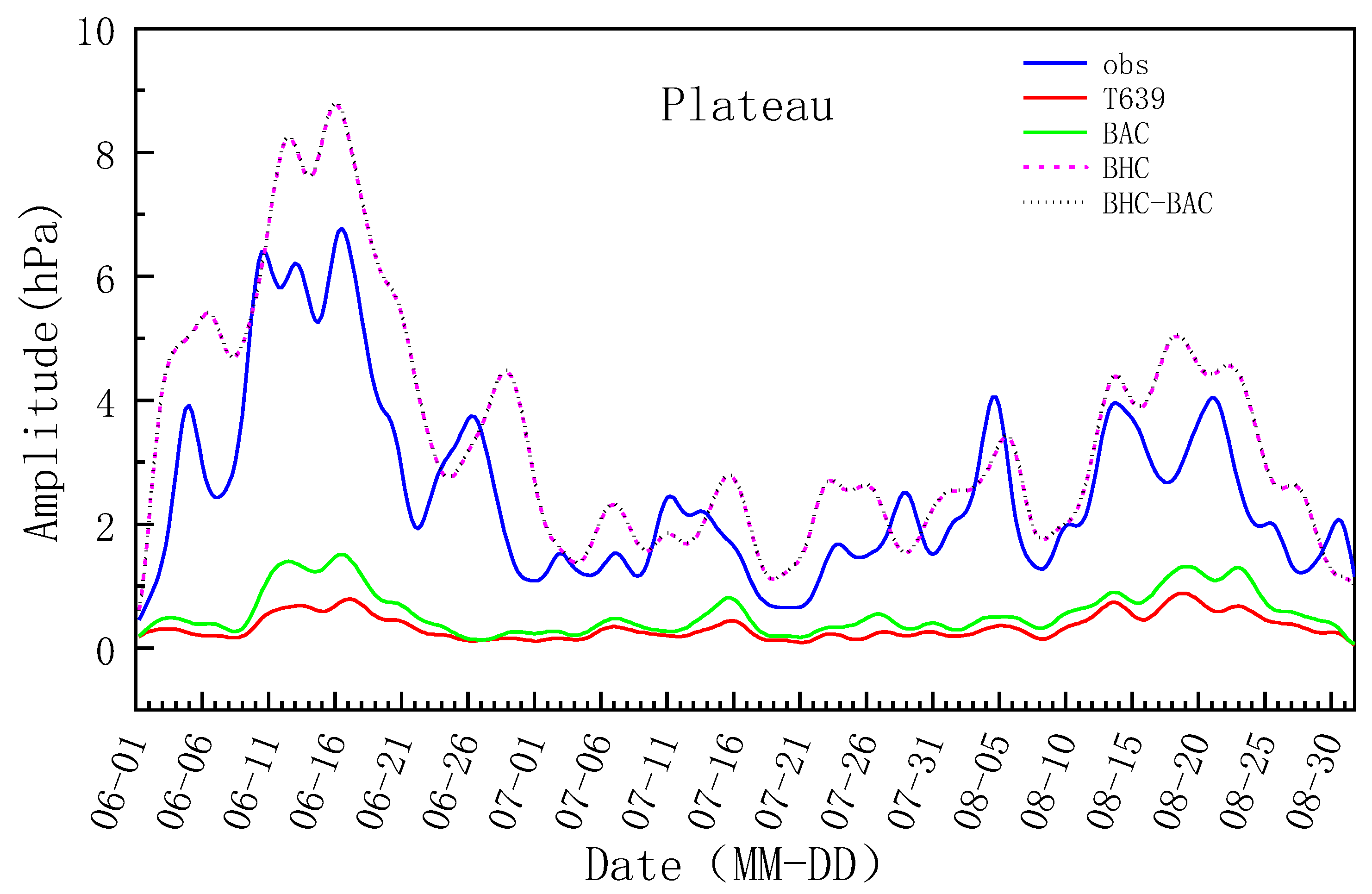
2.2. Analysis Method for the Cycle and Amplitude

Power spectrum analysis can provide the average amplitude, phase, and power contribution of a data series in the whole time domain, and it is widely applied in climatic research. Wavelet analysis shows good local properties in the time and frequency domains and can characterize the amplitude variation over time at a fixed frequency or cycle. In addition, wavelet analysis can be used to analyze the daily variation characteristics of a series, especially the amplitude variation corresponding to the diurnal cycle with time. Therefore, power spectra were used to analyze the series cycle in this study, and wavelet analysis was adopted to analyze the amplitude. The specific calculation methods are shown in Appendix A.

2.3. Progressive EOFs Method

In the progressive EOFs QC method proposed in this research, a simulated observation sequence was added prior to the original observation sequence. Then, the data QC was performed starting from the simulated observation sequence, thus guaranteeing the quality of data in the initial stage of QC. In order to guarantee the performance of QC on the actual observations, the simulated observation sequence should be consistent with the actual observations to ensure a smooth transition to the actual observations. Therefore, the simulated observations must satisfy two basic principles, i.e., the deviations between the simulated observation and background field should meet Gaussian distribution characteristics, and their mean square errors (or standard deviations) should be consistent with those between the observation and background field. In this study, the Gaussian perturbation method was used to simulate observations that satisfied the above two requirements. The method steps are as follows:
First, the T639 surface pressure analysis during 17–31 May (a total of 60 times) was selected to generate simulated observations, and the T639 data were interpolated to observation stations through the bilinear interpolation method. The correction method proposed in this study was used to correct the T639 surface pressure, and the corrected data were expressed as P k , t b , cal ( t = 1 , 2 ,     , 60 ) .
Then, the Gaussian perturbation method was used to generate a Gaussian random sequence. This method was proposed by Box and Muller [32] and improved by Marsaglia and Bray [33] as a polar method. The basic principle of this method is that in the polar coordinate system, the origin is taken as the unit circle center, and a random point series is selected in the unit circle. X and Y denote the horizontal and vertical coordinates of this random series, respectively. The sum of squares of this series can be expressed as S = X 2 + Y 2 . When S 1 or S = 0 , the random points are re-selected until all 60 samples are selected, thus obtaining 60 consistent deviations ( S ) at the interval of (0, 1). Two sets of standard normal distribution random quantities, Z 1 and Z 2 , are generated by Equations (1) and (2).
Z 1 = X 2 ln S S
Z 2 = Y 2 ln S S
Both Z 1 and Z 2 obey standard normal distribution, i.e., the mean values are zero and the standard deviations are 1. Select the first set, Z 1 , as the Gaussian random sequence P k , t Gauss ( t = 1 , 2 ,     , 60 ) .
Finally, the random perturbations, P k , t noise , were generated by the standard deviation product of the Gaussian random sequence P k , t Gauss ( t = 1 , 2 ,     , 60 ) and P k , t obs     P k , t T 639 , cal ( t = 1 , 2 ,     , 368 ; samples during June–August). P k , t T 639 , cal represents the corrected T639 surface pressure analysis. The simulated observations P k , t S - obs ( t = 1 , 2 ,     , 60 ) were generated by adding the random perturbations P k , t noise ( t = 1 , 2 ,     , 60 ) to P k , t b , cal ( t = 1 , 2 ,     , 60 ) .
The Kolmogorov-Smirnov goodness-of-fit method was adopted to test the normality of the simulated observations P k , t S - obs ( t = 1 , 2 ,     , 60 ) , and this normality passed the significance test at the 95% confidence level. Thus, the simulated observations obeyed normal distribution. The observation sequence used in the progressive EOF quality control method was only P k , t obs ( t = 1 , 2 ,     , 368 ) , while that in the progressive EOFs quality control method was the combination of P k , t obs ( t = 1 , 2 ,     , 368 ) and the simulated observation sequence P k , t S - obs ( t = 1 , 2 ,     , 60 ) , where P k , t S - obs ( t = 1 , 2 ,     , 60 ) was in front of P k , t obs ( t = 1 , 2 ,     , 368 ) .

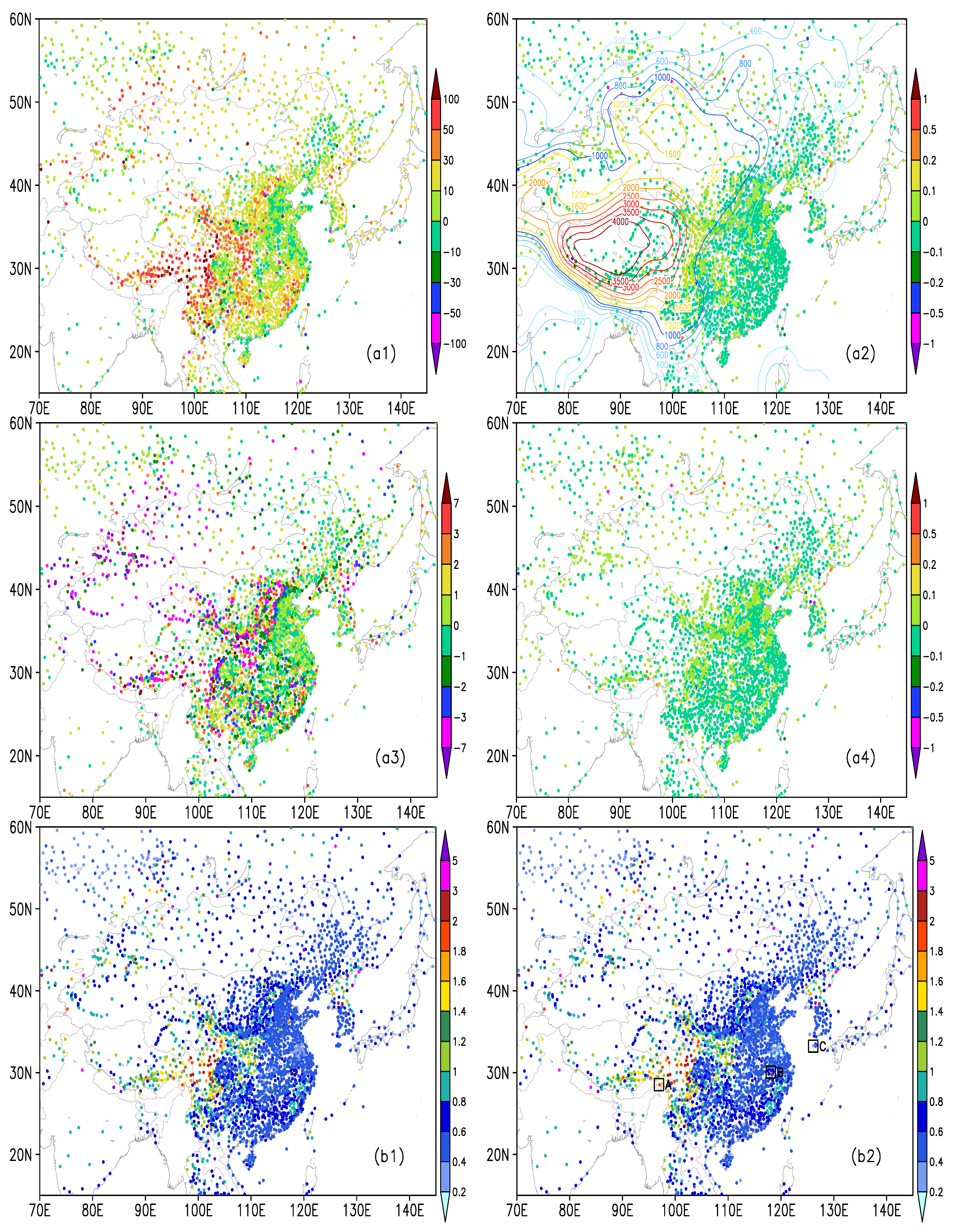
3. Background Correction

The terrain of a model surface is relatively smooth, but there are elevation differences between the model and actual terrain [4]. Therefore, it is necessary to correct the surface pressure analysis (forecast) of the model for surface pressure quality control. The selection of an interpolation correction method is more critical in the Tibetan Plateau with complex topography. Additionally, Liu [31] suggested that there was a great difference in the periodic characteristic of surface pressure from the T639 analysis before and after correction in the Tibetan Plateau. Therefore, the Tibetan Plateau (25° N–40° N, 74° E–104° E) was selected as the study area for analyzing the cycle and amplitude characteristics of surface pressure. In this study, three correction schemes were selected for comparative analysis, namely the barometric height correction (BHC) method [31], the biweight average correction method [27] (BAC), and the method of combining BHC with BAC (BHC-BAC). Note that the principle of the BHC-BAC method is that the BHC method is carried out first, followed by the BAC method.
As presented in Figure 1, the surface pressure observations (4 observation times each day) showed semidiurnal and diurnal cycles in the Tibetan Plateau, corresponding to the frequencies of 0.5000 and 0.2500, respectively. In addition, the observations had an obvious cycle of about 10 days (passing the significance test at the 95% confidence level), and the corresponding frequency was 0.0273. The power spectrum value of the diurnal cycle of the T639 surface pressure was about 10. The spectrum value of the surface pressure observation was about 102. The results in winter were similar to those in summer, and there were also obvious semidiurnal and diurnal cycles. The difference was that there was a long cycle of about 16 days (figure omitted). Therefore, it was necessary to adjust the quality control of the long period sequences by analyzing the long period characteristics of different seasons. The signal strength of the diurnal cycle of the T639 surface pressure was far smaller than that of the observations. The power spectra of the T639 surface pressure before and after correction with the BAC method were basically similar. However, the power spectrum values of the diurnal cycle of the T639 surface pressure corrected by the BHC and BHC-BAC methods exceeded 102, which were larger than those before correction (Figure 1c,d). The semidiurnal cycle signal was also apparently enhanced after correction with the BHC and BHC-BAC methods, and the cycle characteristics were close to those of the observations.
The daily amplitude of the T639 surface pressure data showed a great difference from that of the observations in the Tibetan Plateau, which hardly captured the characteristics of observed daily amplitude (Figure 2). The daily amplitude values of the T639 surface pressure and their variation over time were much smaller than those of the observations, especially during 3–5, 11–21, and 20–26 June, when the daily amplitude of the T639 surface pressure could not catch the variation characteristics of the observed peak amplitude. The daily amplitude of the T639 surface pressure corrected by the BAC method was slightly improved but still much smaller than that of the observations. The daily amplitude of the T639 surface pressure corrected by the BHC and BHC-BAC methods was markedly improved, close to that of the observations. The daily amplitude of the T639 surface pressure corrected by the BAC method differed greatly from the observed amplitude. The daily amplitude of the T639 surface pressure corrected by the BHC and BHC-BAC methods could accurately describe the actual situation, and thus the corrected data could be used for comparison with the surface pressure observations.
Overall, the elevation difference between the model surface and the observation stations cannot be ignored in regions with complex terrains such as the Tibetan Plateau. The results of this study showed that the cycle and amplitude characteristics of the T639 surface pressure corrected by the BHC method were basically consistent with the observations. The T639 surface pressure should have been corrected by the BHC method since the pressure varied nonlinearly with height. Although the BAC method performed well in correcting the 2-m temperature [27], it could not effectively correct the cycle and amplitude of the T639 surface pressure. Therefore, the cycle and amplitude of the T639 surface pressure corrected by the BAC method still showed noticeable differences from the observations.
The performance of the three correction methods was evaluated from the perspective of the daily variation cycle and amplitude above. In the following, the statistical indicators, mean error and root mean square error (RMSE), were also used to evaluate the performance of the three methods to correct the T639 surface pressure, as shown in Figure 3. The results suggested that observation stations with large mean errors between the T639 surface pressure and the observations were distributed with the terrain, i.e., the higher and more complex the topography around the observation stations, the larger the mean errors. Note that the maximum mean error value exceeded 100 hPa. Additionally, the stations with large RMSE values between the T639 surface pressure and the observations were generally distributed with the complex terrain, and these stations were mainly located in large undulating topographic areas, such as western Sichuan and the Tibetan Plateau. The maximum RMSE value was more than 5 hPa. For the T639 surface pressure corrected by the BHC method, the RMSE values were greatly reduced compared with those before correction, and the RMSE values at most stations in complex terrain regions, such as western Sichuan and the Tibetan Plateau, decreased to below 1.2 hPa. In addition, the mean absolute error (MAE) values were also obviously reduced (Table 1), but the magnitude of the reduction was smaller than that for the BAC method. In terms of the T639 surface pressure corrected by the BAC method, the mean errors decreased remarkably compared with those before correction, with values ranging from −0.1 to 0.1 hPa at most stations. However, the RMSE values were almost the same as those before correction. Hence, the BHC method could effectively reduce the RMSE values between the T639 surface pressure and the observations, while the BAC method could obviously decrease the mean errors. The BHC-BAC method could reduce both the mean error and RMSE values, and mean error and RMSE values for the BHC-BAC method were the smallest among the correction results from the three methods. Therefore, the BHC-BAC method achieved the best data correction among the three correction methods.
Further, three representative stations were selected for the 6-h time series analysis of T639 surface pressure and the observations (Figure 4). The three stations are marked as stations A, B, and C. Station A (28.5° N, 97.0° E) had an elevation of 1528 m, while the elevation of the T639 model terrain at this location was 3448.9 m. The elevation of station B (30.1° N, 118.2° E) was 1840 m, while the elevation of the T639 model terrain at this location was 380.5 m. The elevations of station C (33.23° N, 126.55° E) and the corresponding position of the T639 model terrain were 50 and 79.6 m, respectively. At station A, obviously, there was a great difference between the T639 surface pressure and the observations. Specifically, the observations at station A varied between 835 and 850 hPa, with a clear daily cyclic variation. However, the T639 surface pressure was smaller than the observations, ranging from 700 to 705 hPa, with a weak daily cyclic variation. In terms of the mean values, the T639 surface pressure corrected by the BAC method was close to the observations, suggesting that the BAC method could effectively correct the systematic deviations of the T639 surface pressure. However, the daily cyclic variation of the corrected T639 surface pressure was basically consistent with that before correction. The daily cyclic variation characteristic of the T639 pressure data corrected by the BHC method was close to that of the observations, but the corrected values were higher than the observations. Moreover, in terms of the T639 surface pressure corrected by the BHC-BAC method, the daily cyclic variation and values were close to those of the observations. Hence, for the correction of the T639 surface pressure at station A, the corrected values from the BHC-BAC method were the closest to the observations, and thus the BHC-BAC method performed best at station A among the three methods.
From Figure 4b, it could be found that the diurnal cyclic variation characteristic of the surface pressure observed at station B was weaker than that at station A, but the observations at station B showed an apparent long-term periodic variation. The T639 surface pressure at station B was larger than the observations. In contrast, the values of the T639 surface pressure corrected using the three methods were closer to the observations than those before correction. For the T639 surface pressure corrected by the BAC method, there were obvious deviations in some periods. For example, the corrected values on 1–5 and 7–15 June were apparently greater than the observations, while the corrected values on 23–31 July and 5–19 August were obviously less than the observations. Hence, the values corrected by the BHC method were close but slightly smaller than the observations. The values corrected by the BHC-BAC method were the closest to the observations, and thus the correction performance of the BHC-BAC method on the T639 surface pressure at station B was the best.
Compared with the situation in stations A and B, the elevation difference between station C and the corresponding position of the T639 model terrain was relatively small. The diurnal cycle of the observed surface pressure at station C was not apparent, but there was a clear long-term periodic variation similar to station B. In addition, the observations at station C were greater than the T639 surface pressure. The T639 surface pressure corrected by the BAC method was close to the observations, while that corrected by the BHC method was smaller than the observations. Moreover, the T639 surface pressure corrected by the BHC-BAC method was basically consistent with that corrected by the BAC method. In comparison, the correction performance of the BHC-BAC method was still the best at station C among the three correction methods.
The above analysis indicated that the BHC method could effectively reduce the surface pressure deviations between the background field (model analysis or forecast field) and the observations caused by elevation differences, thereby decreasing the RMSE values and mean errors of the surface pressure. The BAC method could obviously reduce the systematic surface pressure deviations between the background field and the observations caused by physical processes and the parameterization schemes of the numerical models, and it could decrease the mean errors of the surface pressure. However, the BAC method showed little improvement in correcting the surface pressure in terms of the RMSE values. The BHC-BAC method integrated the advantages of the BHC and BAC methods, which could effectively reduce the RMSE and mean error values of the surface pressure between the background field and the observations. Hence, the correction performance of the BHC-BAC method was the best. From the time series analysis of single-station observations, it was also found that although the BAC method performed well in correcting systematic deviations, it could not reduce the large differences in cycle and amplitude of the surface pressure between the observations and the background field caused by elevation differences between the model terrain and the actual stations. Therefore, the BHC method was needed to solve this problem. The correction performance of the BHC-BAC method was the best among the three schemes, which made the corrected background field close to the observations, guaranteeing the data quality of the background field used for the quality control of surface pressure.

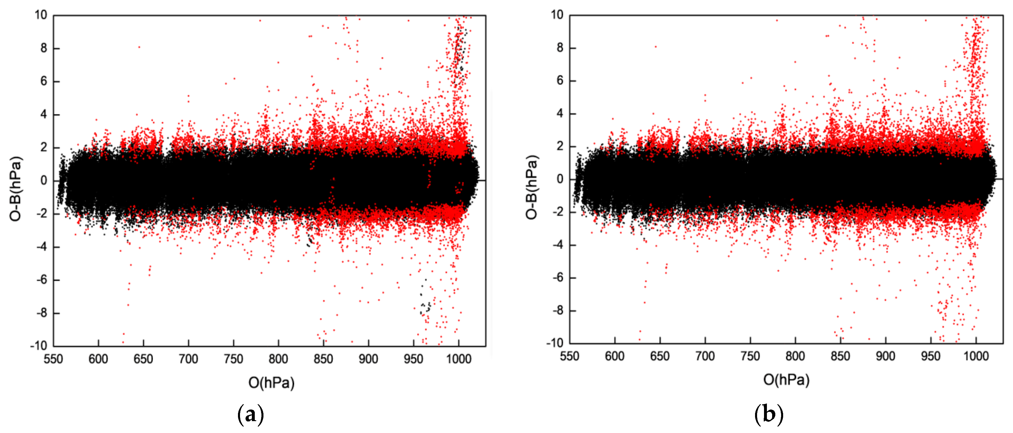
4. Result Analysis of Quality Control

The characteristic analysis of the data in Section 3 revealed that the surface pressure not only had semidiurnal and daily cycles, but it also had a cycle of about 10 days (passing the significance test at the 95% confidence level). Thereby, the progressive EOF and EOFs methods used in this study took 10 days as a cycle, i.e., 40 time data as a set, to calculate the EOF. The explained variance of the first mode was more than 99%, indicating that the first mode could better characterize the daily and semidiurnal cycles of the surface pressure. Thus, the first mode was selected to reconstruct the data series. The simulated observations used in the EOFs method were generated from background fields greater than one cycle.
Figure 5 shows the biweight standard deviations of the P k , t obs     P k , t T 639 , cal after quality control by the progressive EOF and EOFs methods. The biweight standard deviations from the two quality control methods were the same, indicating that the simulated observations met the quality control requirements. The biweight standard deviations of the P k , t obs P k , t T 639 , cal showed an east–west distribution, i.e., larger biases were concentrated in the area west of 110° E, and smaller biases were mainly distributed in the area east of 110° E. This result was different from the north–south division of the 2-m temperature [34]. In the region with large biweight standard deviations, the difference between the observations and the background field was large. In order to better match the observations with the background field, more outliers should be removed in areas with large biweight standard deviations, and vice versa. The Z-score was 3.5 in the area west of 110° E and 4.0 in the area east of 110° E.
Quality control should both eliminate as many outliers as possible and should retain as much correct data that characterizes anomalous atmospheric conditions as possible. Figure 6 shows the deviation scatter plots of the data eliminated by the progressive EOF and EOFs quality control methods. The data rejection rate of the progressive EOF method was 0.74%, and that of the progressive EOFs method was 0.77%. Thus, the amount of data eliminated by the progressive EOFs method was slightly more than that of the progressive EOF method. From Figure 6, it could be found that the absolute values of the P obs P T 639 , cal deviations eliminated by the progressive EOF method were generally more than 2 hPa. The eliminated data were basically the data with large deviations between the T639 surface pressure and the observations. The deviations between the rejected and background data fluctuated slightly at different altitudes, which may have been due to the variable sliding standard used in the progressive EOF method to reject data. Figure 6a shows that the progressive EOF method retained a small number of observations with absolute values of the deviation exceeding 4 hPa, while it unreasonably rejected some observations with absolute values of the deviation less than 1 hPa. When the simulated observations were used in the progressive EOFs method for quality control, these unreasonable phenomena did not exist (Figure 6b).
From the time series of the data elimination percentages of the progressive EOF and EOFs methods from 1 June to 16 July 2013 (Figure 7), it could be found that the data rejection rate of the progressive EOFs method was higher than that of the progressive EOF method in the initial stage (before June 10) of quality control. After June 10, the elimination percentages of the two quality control methods were close, indicating that the difference in quality control performance between the progressive EOFs and EOF methods was mainly in the early stage of quality control.
Figure 8 presents the skewness and kurtosis coefficients of the P EOF res obs P EOF res T 639 , cal before and after quality control using the progressive EOF and EOFs methods. P EOF res obs and P EOF res T 639 , cal respectively indicate the residual terms of the observations and the T639 surface pressure, as detailed in the introduction of the progressive EOF quality control method [27] The results showed that for both the progressive EOF and EOFs methods, the skewness coefficient of the data after the background correction by the BHC-BAC method and quality control was closer to 0 than before correction, and the kurtosis coefficient was closer to 3. The kurtosis and skewness coefficients for the two methods were similar.
The difference in the rejection rate between the progressive EOF and EOFs methods mainly appeared in the initial stage of quality control, with little impact on quality control in the later stage. Therefore, the spatial distribution of the data rejection rates of the two quality control methods was quite similar (Figure 9), mainly showing that the data rejection rate was relatively low in the eastern region and high in the western region. In addition, the stations with data rejection rates higher than 3% were located in areas with large RMSE values, such as western Sichuan, the Tibetan Plateau, northern Xinjiang, and the surrounding regions with complex terrain.
Four representative stations with large differences in the data rejection rates of the two quality control methods were selected to analyze the time series of the surface pressure. These stations are marked in Figure 9 as stations A (38.4° N, 127.3° E; 352 m a.s.l.), B (38.5° N, 126.5° E; 97 m a.s.l.), C (28.2° N, 116.82° E; 47 m a.s.l.), and D (44.17° N, 87.97° E; 547 m a.s.l.).
Figure 10 indicates that there was a difference in the quality control performance between the progressive EOF and EOFs methods. The absolute O-B values of surface pressure at station A were relatively large from 0000 UTC on 1 June to 1200 UTC on 7 June, with most of the absolute O-B values greater than 5 hPa. The absolute O-B values were less than 1 hPa from 1800 UTC on 7 June to 0000 UTC on 13 June, especially at 1800 UTC on 7 June (only 0.3 hPa). The progressive EOF method identified and rejected (indicated by green and blue dots) some outliers from 0000 UTC on 1 June to 1200 UTC on 7 June, while it identified and rejected all observation data as outliers in the period from 1800 UTC on 7 June to 0000 UTC on 13 June. The progressive EOFs method identified and rejected all of the observation data with large absolute O-B values during 1–7 June, while it retained the observations with small absolute O-B values in the subsequent period. After 0000 UTC on 13 June, the two methods had the same effect on identifying outliers, both for observations with large absolute O-B values.
The time series of the observations at station B showed that the data at this station were incorrect. The observations were larger than the T639 surface pressure before 16 July, while they decreased rapidly after 16 July and were far smaller than the T639 surface pressure. Most absolute O-B values were above 5 hPa before 25 June and above 15 hPa after 16 July. Although the progressive EOF and EOFs methods had the same elimination effect on the observations at station B in the later period, the progressive EOF method performed worse before 0000 UTC on 15 June, rejecting only a small number of outliers. In contrast, the progressive EOFs method identified all of the outliers, showing a better effect on quality control.
The absolute O-B values at station C were mostly above 5 hPa before 1800 UTC on 4 June, and both quality control methods were able to identify the outliers in this period. However, the progressive EOF method also rejected the outliers with small absolute O-B values in the subsequent period. This unreasonable phenomenon did not appear when using the progressive EOFs method. At station D, the difference in surface pressure between the observations and T639 surface pressure was small, and the results of the two quality control methods were similar. Specifically, the absolute O-B values of the outliers eliminated using the progressive EOF method alone were 1.8 hPa, while those eliminated using the progressive EOFs method alone were 2.2, 2.3, 3.0, and 2.7 hPa. Hence, using the progressive EOFs method to reject outliers was more reasonable.
Overall, when the observations had continuous outliers with the same characteristic at the initial stage of quality control, the progressive EOF method could not effectively identify outliers, which may have affected data quality control in the subsequent period. Nevertheless, this unreasonable phenomenon did not appear when using the progressive EOFs method, mainly because the progressive EOF method used the reconstructed residual field P EOF res obs P EOF res T 639 , cal (mainly including certain random errors) to identify outliers. The progressive EOF method assumed only a few outliers in the samples. Suppose there were continuous outliers with the same characteristic in the initial stage of quality control at a station. In that case, the progressive EOF method considered that the samples consisting of these outliers were correct and they were retained. These retained outliers could cause the correct data to be identified as outliers and rejected in the next period. In the progressive EOFs method, the background-based simulated observations with matching observation characteristics were sequenced in front of the observation series. Thus, the progressive EOFs method effectively avoided the influence of continuous outliers with the same characteristic at the initial stage of quality control, ensuring the data quality in the whole period.

5. Conclusions and Discussion

In this study, we analyzed the cycle and amplitude characteristics of the 6-h T639 surface pressure data (background field) and observations on the Tibetan Plateau from June to August 2013. Using different correction methods, we corrected the background field from the elevation of the model surface to that of the observation stations. Based on this, a progressive EOFs quality control method based on the BHC-BAC method was proposed in this research for the quality control of surface pressure data. The main conclusions are as follows.
The daily variation cycle and amplitude characteristics of the observed surface pressure and the T639 surface pressure are inconsistent on the Tibetan Plateau, and the T639 analysis field can hardly describe the diurnal variation cycle and amplitude of the observations due to elevation differences between the model terrain and the observation stations. After correcting the T639 surface pressure from the model surface to the elevation of the observation stations using the BHC or BHC-BAC methods, the cycle and amplitude characteristics of the corrected data showed good consistency with the observations. For the T639 surface pressure corrected by the BAC method, the diurnal variation amplitude was slightly improved while the cycle characteristics remained essentially the same as before correction, which were obviously different from the observations.
The BHC method could effectively reduce the deviations and RMSE values between the background field and the observations caused by elevation differences. The BAC method could obviously decrease the systematic deviations caused by physical processes and the parameterization schemes of models, and it could greatly reduce the mean errors. However, the BAC method could not decrease the RMSE values. The BHC-BAC method integrated the advantages of the BHC and BAC methods, which could effectively reduce the RMSE and mean error values between background field and the observations. Thus, the correction performance of the BHC-BAC method was the best.
The results of quality control using the progressive EOF and EOFs methods were close to normal distribution. The two quality control methods had similar spatial distributions of the data rejection rate, and the elimination percentage in the eastern region was lower than that in the western region. In addition, the data rejection rate of the progressive EOFs method was slightly higher than that of the progressive EOF method.
When there were outliers with the same characteristics at the initial stage of quality control, the progressive EOF method could unreasonably reject observation data. The progressive EOFs method effectively solved this problem, and the quality control effect in the subsequent period was not affected. Therefore, the progressive EOFs method performed better than the progressive EOF method.
The BHC and BHC-BAC methods can be applied not only to the quality control and assimilation scheme of surface pressure, but also to the processing of surface pressure products for model analysis and forecasting. The differences in the results of the quality control methods between the 2-m temperature and the surface pressure indicate that the quality control of different observations and elements should be carried out based on an analysis and understanding of the data characteristics. Developing corresponding quality control methods according to the data characteristics is necessary rather than applying them directly. There are still some shortcomings in this study. In the next step, it is necessary to conduct research on observation stations with high missing test rates, combine model background analysis and AI-based methods with alternate missed observation values, and use data assimilation experiments to test the effect of improving quality control. Moreover, we need to carry out corresponding research on different cycle and amplitude characteristics in different seasons.

Author Contributions

Conceptualization, P.L. and Z.X.; data curation, P.L. and Z.X.; formal analysis, Z.X.,P.L., J.G. and W.C.; funding acquisition, Z.X. and J.G.; investigation, P.L. and Z.X.; methodology, Z.X., P.L. and J.G.; project administration, Z.X. and J.G.; resources, Z.X. and J.G.; software, P.L.; supervision, J.G.; validation, P.L.; visualization, P.L. and Z.X.; writing—original draft, P.L. and Z.X.; writing—review and editing, P.L., Z.X., J.G. and W.C. All authors have read and agreed to the published version of the manuscript.

Funding

This research was supported by the National Natural Science Foundation of China (No. 41275105) and Science and Technology Development Fund Project of Hubei Meteorological Bureau (No.2022Y16, No.2023Y11).

Institutional Review Board Statement

Not applicable.

Informed Consent Statement

Not applicable.

Data Availability Statement

The 6-h surface observations and the T639 (T639L60 Global Medium Range Forecast System, 0.28125° × 0.28125°) analysis from June to August 2013 are used in this research. These data were obtained from China’s National Meteorological Center.

Acknowledgments

We thank Y. Wang for his help and guidance on the progressive EOF quality control method and Nanjing Hurricane Translation for reviewing the English language quality of this paper.

Conflicts of Interest

The authors declare no conflict of interest.

Appendix A

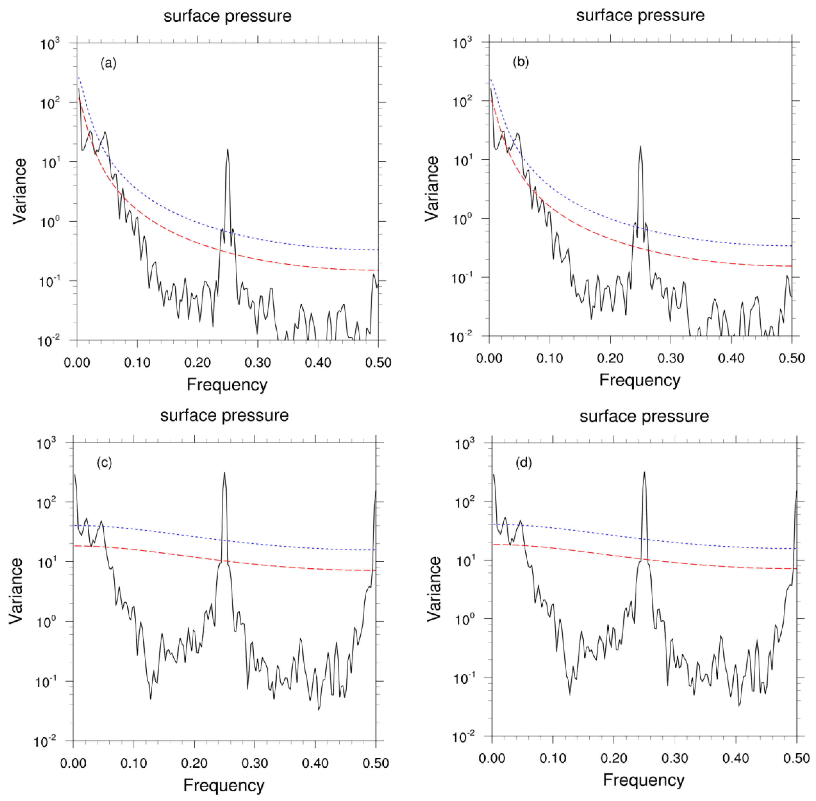
Appendix A.1. Power Spectrum Analysis

Power spectra can diagnose the main cycle of the sequence, and frequency–domain analysis based on the Fourier transform can decompose the total energy of the sequence into different frequency domains. Then, the main period of the sequence is diagnosed according to the wave power (variance contribution) with different frequencies.
The specific calculation process is as follows, and the algorithm refers to Wei [35]. Here, the summer surface pressure observations on the Tibetan Plateau are taken as an example, and there were 216 stations in this area. Firstly, the average value P t obs of the surface pressure in this area at each time is calculated. Then, the correlation coefficient r ( j ) is calculated using Equation (A1).
r ( j ) = 1 n - j i = 1 n ( P t obs     P - obs s P t obs ) ( P i + j obs P - obs s P t obs ) ,   j   =   0 , 1 , 2 ,     , m
where n (368) denotes the sample size of the time series P t obs ; P - obs is the average value of P t obs ; and s P t obs is the standard deviation of P t obs . The maximum lag time length m is taken as 40 in this section, and its range is between n 10 and n 3 . r j represents the correlation coefficient at the j th time interval. The rough spectrum estimates of different wavenumbers k are calculated using Equations (A1) and (A2).
s k = 1 m r 0 + 2 j = 1 m 1 r j cos k π j m + r m cos k π ,   k = 0 , 1 , , m
Finally, the power spectrum estimates S ^ k obtained by Equations (A1)–(A3) are processed with the Hanning smoothing coefficient, as given by Equation (A4).
s 0 = 1 2 m r 0 + r m + 1 m j = 1 m 1 r j s k = 1 m r 0 + 2 j = 1 m 1 r j cos k π j m + r m cos k π s m = 1 2 m r 0 + 1 m   r m 1 m j = 1 m 1 1 j   r j
s 0 = 0.5 s ^ 0 + 0.5 s ^ 1 s k = 0.25 s ^ k 1 + 0.5 s ^ k + 0.25 s ^ k + 1 s m = 0.5 s ^ m 1 + 0.5 s ^ m
Determination of the cycle: when m is large, there is a sharp spectral peak of the spectral estimates near a certain frequency, while the power spectral values are relatively small at other frequencies. In this case, the reciprocal of the frequency corresponding to this spectral peak is the implied cycle [36]. The relationship of the cycle T k with wavenumber k is T k = 2 m k .

Appendix A.2. Wavelet Analysis

The wavelet analysis method has good local properties in the time and frequency domains. In addition, it can analyze the local characteristics of periodic variations of a time series, thereby more clearly characterizing the variation of each cycle over time. The algorithm refers to Wei [35] and Wu [37]. Morlet wavelets are generated because of the amplitudes of the sine and cosine waves being modulated by Gaussian functions. In this section, the standard Morlet wavelets are selected as the mother wavelet, as given by Equation (A5).
ψ t = e i 2 π t e t 2 2
The continuous form of the mother wavelet is as follows (Equation (A6)).
w a , b = x , Ψ a , b = a 1 2 x t Ψ * t b a d t
where the symbol ( , ) represents the inner product, * is the conjugate, a is the expansion scale, b is the translation parameter, and x t is the analyzed object.
f ( t ) = x ( t ) x ¯ ( t ) s ( t )
where x ¯ ( t ) denotes the average value of x t , s ( t ) the standard deviation of x t , and w a , b the wavelet coefficient. The discrete expression is as follows (Equation (A8)).
w a , b = f , Ψ a , b = a 1 2 Δ t i = t n f i Δ t Ψ * i Δ t b a
where Δ t represents the sampling interval, and n indicates the sample size. The discrete wavelet transform forms the normal orthogonal system, which expands the field of practical applications. In this study, the modulus of wavelet coefficient w a , b is collectively referred to as amplitude [37], and its unit is dimensionless.
Wavelet analysis can show the variations of amplitude and power contribution over time for a given frequency or cycle.

References

  1. Zhang, H. The importance of analyzing data from automatic stations for weather Forecasting. Agric. Technol. 2012, 32, 124. (In Chinese) [Google Scholar] [CrossRef]
  2. Zhang, Y.C.; Yao, R.J.; Xiong, X.; Shen, Y.P. Application of PSO-PSR-ELM-based ensemble learning algorithm in quality control of surface temperature observations. Clim. Environ. Res. 2017, 22, 59–70. (In Chinese) [Google Scholar] [CrossRef]
  3. Xu, H.R. The disadvantage and countermeasure of surface meteorological observation automation. Henan Sci. Technol. 2019, 22, 151–152. (In Chinese) [Google Scholar]
  4. Xu, Z.F.; Gong, J.D.; Wang, J.J.; Li, Z.C. A study of assimilation of surface observational data in complex terrain part I: Influence of the elevation difference between model surface and observation site. Chin. J. Atmos. Sci. 2007, 31, 222–232. (In Chinese) [Google Scholar]
  5. Zhang, L.H.; Du, Q.; Chen, J.; Xiao, Y.H. Sensitive experiments of surface observation data in numerical weather precipitation over southwestern China. Meteorol. Mon. 2009, 35, 26–35. (In Chinese) [Google Scholar]
  6. Xue, J.S. Scientific issues andperspective of assimilation of meteorological satellite data. Acta Meteorol. Sin. 2009, 67, 903–911. (In Chinese) [Google Scholar] [CrossRef]
  7. Jia, B.X.; Xu, H.M.; An, Y.G. Comparisons of atmospheric specific humidity in reanalysis datasets and homogenized radiosonde dataset in China. Meteorol. Mon. 2014, 40, 1123–1131. (In Chinese) [Google Scholar] [CrossRef]
  8. Liu, X.N.; Ren, Z.H. Progress in quality control of surface meteorological data. Meteorol. Sci. Technol. 2005, 33, 199–203. (In Chinese) [Google Scholar] [CrossRef]
  9. Ye, X.L.; Chen, Y.; Yang, S.; Yang, X.; Kan, Y.J. A quality control method of surface temperature observations based on the EEMD-CES algorithm for a single station. Trans. Atmos. Sci. 2019, 42, 390–398. (In Chinese) [Google Scholar] [CrossRef]
  10. Tao, S.W.; Zhong, J.Q.; Xu, Z.F.; Hao, M. Quality control schemes and its application to automatic surface weather observation system. Plateau Meteorol. 2009, 28, 1202–1209. (In Chinese) [Google Scholar]
  11. Wang, H.J.; Yan, Q.Q.; Xiang, F.; Meng, P. Algorithm design of quality control for hourly air temperature. Plateau Meteorol 2014, 33, 1722–1729. (In Chinese) [Google Scholar] [CrossRef]
  12. Shafer, M.A.; Fiebrich, C.A.; Arndt, D.S.; Fredrickson, S.E.; Hughes, T.W. Quality assurance procedures in the oklahoma mesonet work. J. Atmos. Ocean. Technol. 2000, 17, 474–494. [Google Scholar] [CrossRef]
  13. Reek, T.; Doty, S.R.; Owen, T.W. A deterministic approach to the validation of historical daily temperature and precipitation data from the cooperative network. Bull. Am. Meteorol. Soc. 1992, 73, 753–762. [Google Scholar] [CrossRef]
  14. Eischeid, J.K.; Baker, C.B.; Karl, T.R.; Diaz, H.F. The quality control of long-term climatological data using objective data analysis. J. Appl. Meteorol. 1995, 34, 2787–2795. [Google Scholar] [CrossRef]
  15. Xiong, X.; Tang, H.S.; Zhang, Y.C.; Ye, X.L. A spatial consistency quality control method for daily surface temperature observations. J. Trop. Meteorol. 2020, 26, 461–472. [Google Scholar] [CrossRef]
  16. Dee, D.P.; Rukhovets, L.; Todling, R.; Silva, A.M.; Larson, J.W. An adaptive buddy check for observational quality control. Q. J. R. Meteorol. Soc. 2001, 127, 2451–2471. [Google Scholar] [CrossRef]
  17. Ren, Z.H.; Xiong, A.Y. Operational system development on three-step quality control of observations from AWS. Meteorol. Mon. 2007, 33, 19–24. (In Chinese) [Google Scholar]
  18. Hui, W.; Wang, X.L.; Swail, V.R. A Quality Assurance System for Canadian Hourly Pressure Data. J. Appl. Meteorol. 2007, 46, 1804–1817. [Google Scholar] [CrossRef]
  19. Xu, Z.F.; Chen, X.J.; Chen, Y. Quality control scheme for new-built automatic surface weather observation station’s data. Sci. Meteorol. Sin. 2013, 33, 26–36. (In Chinese) [Google Scholar] [CrossRef]
  20. Jiang, H.; Xu, W.H.; Yang, S.; Zhu, Y.; Zhou, Z.J.; Liao, J. Development of an integrated global land surface dataset from 1901 to 2018. J. Meteorol. Res. 2021, 35, 789–798. [Google Scholar] [CrossRef]
  21. Li, L.F.; Wang, H.J.; Liu, J.Y.; Song, S. Surface meteorological data quality control based on blackboard model. Meteorol. Sci. Technol. 2006, 34, 199–204. (In Chinese) [Google Scholar] [CrossRef]
  22. Zhou, X.T.; Chu, X.; Yao, Z.P. A dynamic method of quality control for real-time temperature measurements based on k-means clustering algorithm. Meteorol. Mon. 2012, 38, 1295–1300. (In Chinese) [Google Scholar]
  23. Ye, X.L.; Shi, L.H.; Xiong, X.; Wang, L. Application of AI method to quality control in surface temperature observation data. Clim. Environ Res. 2016, 21, 1–7. (In Chinese) [Google Scholar] [CrossRef]
  24. Zheng, W.Z.; Wei, H.; Meng, J.; EK, M.; Mitchell, K.; Derber, J.; Zeng, X.B.; Wang, Z. Improvement of land surface skin temperature in NCEP operational NWP Models and its impact on satellite data assimilation. In Proceedings of the 23rd Conference on Weather Analysis and Forecasting/19th Conference on Numerical Weather Prediction, Omaha, NE, USA, 1–5 June 2009. [Google Scholar]
  25. Han, L.; Chen, M.X.; Chen, K.K.; Chen, H.N.; Zhang, Y.; Lu, B.; Song, L.; Qin, R. A deep learning method for bias correction of ECMWF 24–240 h forecasts. Adv. Atmos. Sci. 2021, 38, 1444–1459. [Google Scholar] [CrossRef]
  26. Qin, Z.K.; Zou, X.L.; Li, G.; Ma, X.L. Quality control of surface station temperature data with non-Gaussian observation-minus-background distributions. J. Geophys. Res. 2010, 115, D16312. [Google Scholar] [CrossRef] [Green Version]
  27. Xu, Z.F.; Wang, Y.; Fan, G.Z. A two-stage quality control method for 2-m temperature observations using biweight means and a progressive EOF analysis. Mon. Weather Rev. 2013, 141, 798–808. [Google Scholar] [CrossRef]
  28. Zhao, H.; Qin, Z.K.; Wang, J.C.; Liu, Y. Case studies and applications of the Empirical Orthogonal Function: Quality control in variational data assimilation systems for surface observation data. Acta Meteorol. Sin. 2015, 73, 749–765. (In Chinese) [Google Scholar] [CrossRef]
  29. Shen, W.B.; Li, X.; Qin, Z.K.; Zhang, B. Restoration method for automatic station temperature observation data based on EOF iteration. J. Atmos. Sci. 2022, 46, 406–418. (In Chinese) [Google Scholar] [CrossRef]
  30. Shao, Y.H.; Qin, Z.K.; Li, X. Quality control based on EOF for surface temperature observations from high temporal-spatial resolution automatic weather stations. Trans Atmos Sci. 2022, 45, 603–615. (In Chinese) [Google Scholar] [CrossRef]
  31. Liu, P.T.; Xu, Z.F.; Xu, K.Y.; Wang, J.; Li, Z.C. Study of surface progressive OMB pressure quality control for data assimilation. Meteorol. Mon. 2017, 43, 1138–1151. (In Chinese) [Google Scholar] [CrossRef]
  32. Box, G.E.; Muller, M.E. A note on the generation of random normal deviates. Ann. Math. Stat. 1958, 2, 610–611. [Google Scholar] [CrossRef]
  33. Marsaglia, G.; Bray, T.A. A convenient method for generating normal variables. SIAM Rev. 1964, 6, 260–264. [Google Scholar] [CrossRef]
  34. Wang, Y.; Xu, Z.F.; Fan, G.Z. Study of EOF quality control method of 2m temperature. Plateau Meteorol. 2013, 32, 564–574. (In Chinese) [Google Scholar] [CrossRef]
  35. Wei, F.Y. Modern Climate Statistical Diagnosis and Prediction Technology, 2nd ed.; China Meteorological Press: Beijing, China, 2007; pp. 77–81. (In Chinese) [Google Scholar]
  36. Tang, J. Periodicity analysis based on power spectrum estimation. J. Shaanxi Univ. Technol. Nat. Sci. Ed. 2013, 29, 74–78. (In Chinese) [Google Scholar]
  37. Wu, H.B.; Wu, L. Methods for Diagnosing and Forecasting Climate Variability; China Meteorological Press: Beijing, China, 2005; pp. 237–254. (In Chinese) [Google Scholar]
Figure 1. Power spectra of the T639 surface pressure before (a) and after correction with the (b) BAC, (c) BHC, and (d) BHC-BAC methods, and (e) power spectrum of surface pressure observations. The black lines indicate power spectrum, the blue short-dotted lines represent the spectra passing the significance test at the 95% confidence level, and the red long-dashed lines denote the red noise power spectra. Units of frequency are day−1, and those of variance are hPa2.
Atmosphere 14 01032 g001aAtmosphere 14 01032 g001b
Figure 2. Amplitude variation of the T639 surface pressure diurnal cycle before and after correction with the BAC, BHC, and BHC-BAC methods, and the daily amplitude variation of surface pressure observations (obs).
Atmosphere 14 01032 g002
Figure 3. Distributions of the (a1a4) mean error (unit: hPa) and (b1b4) RMSE values (unit: hPa) between the observations and T639 surface pressure (a1,b1) before and after correction by the (a2,b2) BAC method, (a3,b3) BHC method, and (a4,b4) BHC-BAC methods. The color contours in (a2) represent the station terrain (unit: m). The boxes A–C in (b2) indicate three representative stations with corrected T639 surface pressure results described in this study.
Atmosphere 14 01032 g003aAtmosphere 14 01032 g003b
Figure 4. The 6-h time series of the observations and T639 surface pressure at stations A (a), B (b), and C (c) before and after correction with the BAC, BHC, and BHC-BAC methods. The right coordinates indicate the T639 surface pressure before correction, and the left coordinates denote the corrected results.
Atmosphere 14 01032 g004
Figure 5. Biweight standard deviations (unit: hPa) of the P k , t obs P k , t T 639 , cal from the (a) progressive EOF method and (b) progressive EOFs method.
Atmosphere 14 01032 g005
Figure 6. Scatter plots of P obs P T 639 , cal (O-B) and observations (O) before and after quality control by the progressive EOF (a) and EOFs (b) methods. Black dots denote the retained data, and red dots indicate the excluded outliers.
Atmosphere 14 01032 g006
Figure 7. Time series of the data elimination percentages of the progressive EOF and EOFs methods.
Atmosphere 14 01032 g007
Figure 8. Skewness and kurtosis coefficients of P EOF res obs P EOF res T 639 , cal before and after quality control using the progressive EOF and EOFs methods.
Atmosphere 14 01032 g008
Figure 9. Spatial distribution of data rejection rates (unit: %) of the (a) progressive EOF and (b) EOFs methods. Boxes A–D indicate four representative stations with quality control results described in this paper.
Atmosphere 14 01032 g009
Figure 10. Time series of the observations at stations (a) A, (b) B, (c) C and (d) D, corrected T639 surface pressure (hollow circles) and observation data rejected by the progressive EOF method (red dots), progressive EOFs method (green dots), and both quality control methods (blue dots).
Atmosphere 14 01032 g010aAtmosphere 14 01032 g010b
Table 1. Statistics of the observation stations with large MAE or RMSE values before and after correction.
Before and after CorrectionMAE
(Unit: hPa)
MAE
(Number of Observation Stations)
RMSE
(Unit: hPa)
RMSE
(Number of Observation Stations)
Without Correction305540.8776
BAC0.1480.8652
BHC34750.8317
BHC-BAC0.1410.8317
Disclaimer/Publisher’s Note: The statements, opinions and data contained in all publications are solely those of the individual author(s) and contributor(s) and not of MDPI and/or the editor(s). MDPI and/or the editor(s) disclaim responsibility for any injury to people or property resulting from any ideas, methods, instructions or products referred to in the content.

