

The Distribution and Impact Characteristics of Small-Scale Carbon Emissions in the Chengdu–Chongqing Region
Abstract
:1. Introduction
- (1)
- From the perspective of research objects, previous studies mostly focused on carbon emissions in the Yangtze River Delta, Pearl River Delta, Beijing–Tianjin–Hebei and other economically developed areas [38,39,40]. With the implementation of Western development and the “the Belt and Road Initiatives” and additional strategies, the contribution of the western region to China’s carbon emissions has gradually increased [41,42], but there are relatively few studies on carbon emissions in the western region, especially in the national emerging town clusters such as the Chengdu–Chongqing region. In addition to the lack of statistical data of energy utilization at the county level, there is no research on the detailed analysis of carbon emissions in the Chengdu–Chongqing region from the county perspective.
- (2)
- From the perspective of research ideas, existing studies reveal the impact of a single factor on carbon emissions in a simple way, the use of the geographical detector model to analyze the interaction of carbon emissions impact factors is low, and most of the relevant studies ignore the development stage and regional differences, revealing that the spatio-temporal heterogeneity of the influencing factors is relatively lacking.
- (1)
- Analyze carbon emissions in the Chengdu–Chongqing region from the county scale to improve the detailed study of carbon emissions in western China.
- (2)
- Reveal the spatio-temporal differences of the single and interactive factors affecting carbon emissions to fill the lack of studies on the spatio-temporal differences of influencing factors.
2. Study Area and Methodology
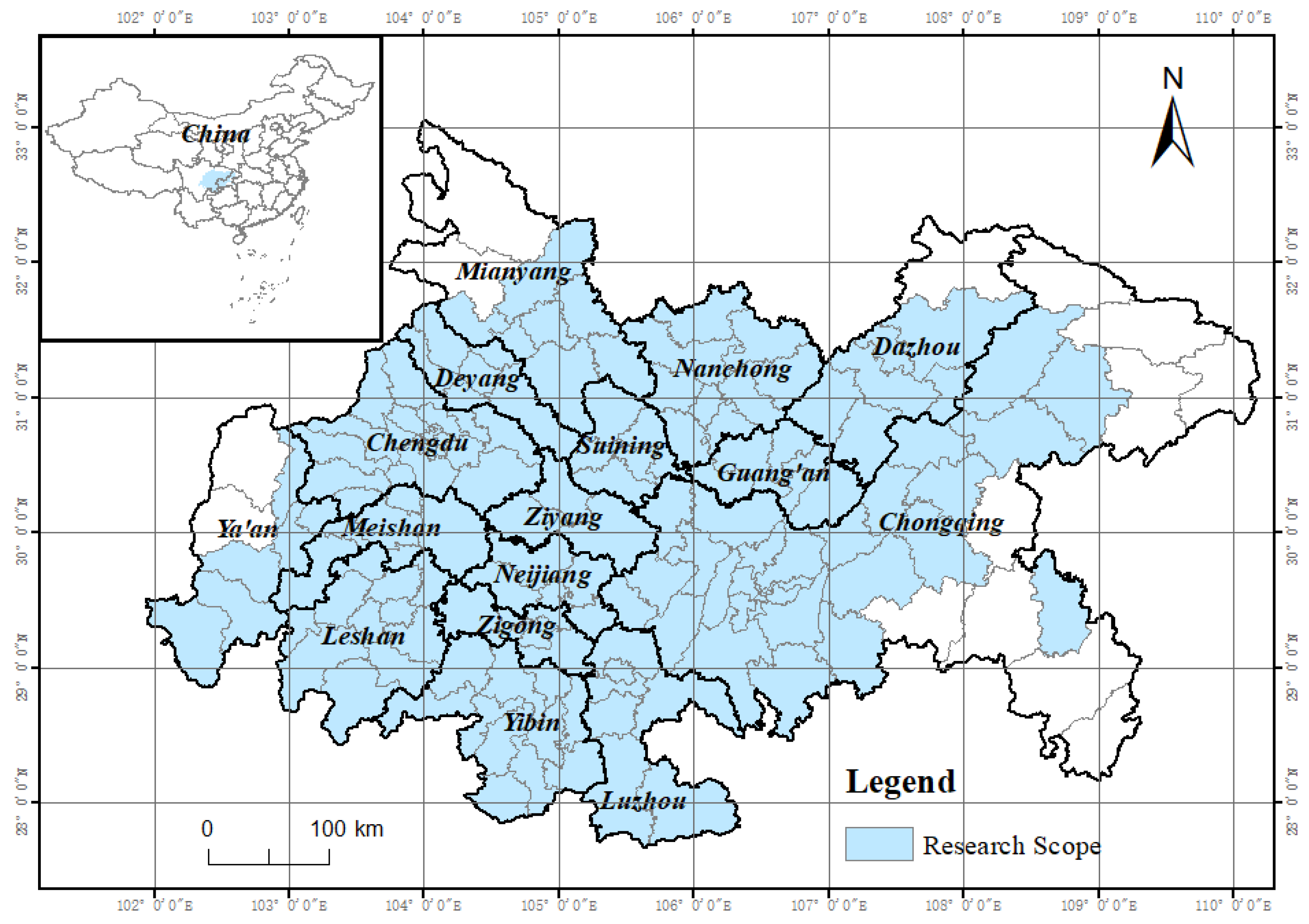
2.1. Study Area
2.2. Research Methodology
2.2.1. Spatial and Temporal Evolution Analysis Model of Carbon Emissions
2.2.2. Analysis Model of Carbon Emission Influencing Factors
- (i).
- The factor detector
- (ii).
- The interaction detector
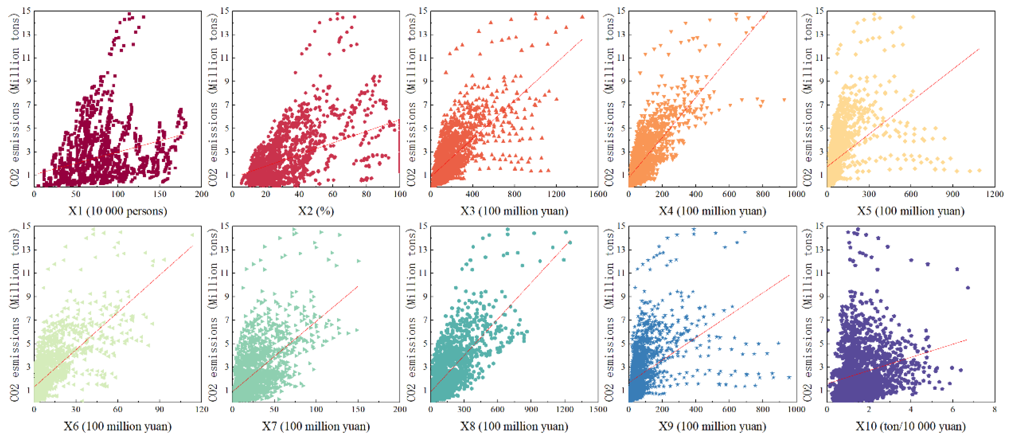
2.3. Data Sources
3. Results
3.1. Spatial and Temporal Distribution of Carbon Emissions in the Chengdu–Chongqing Region
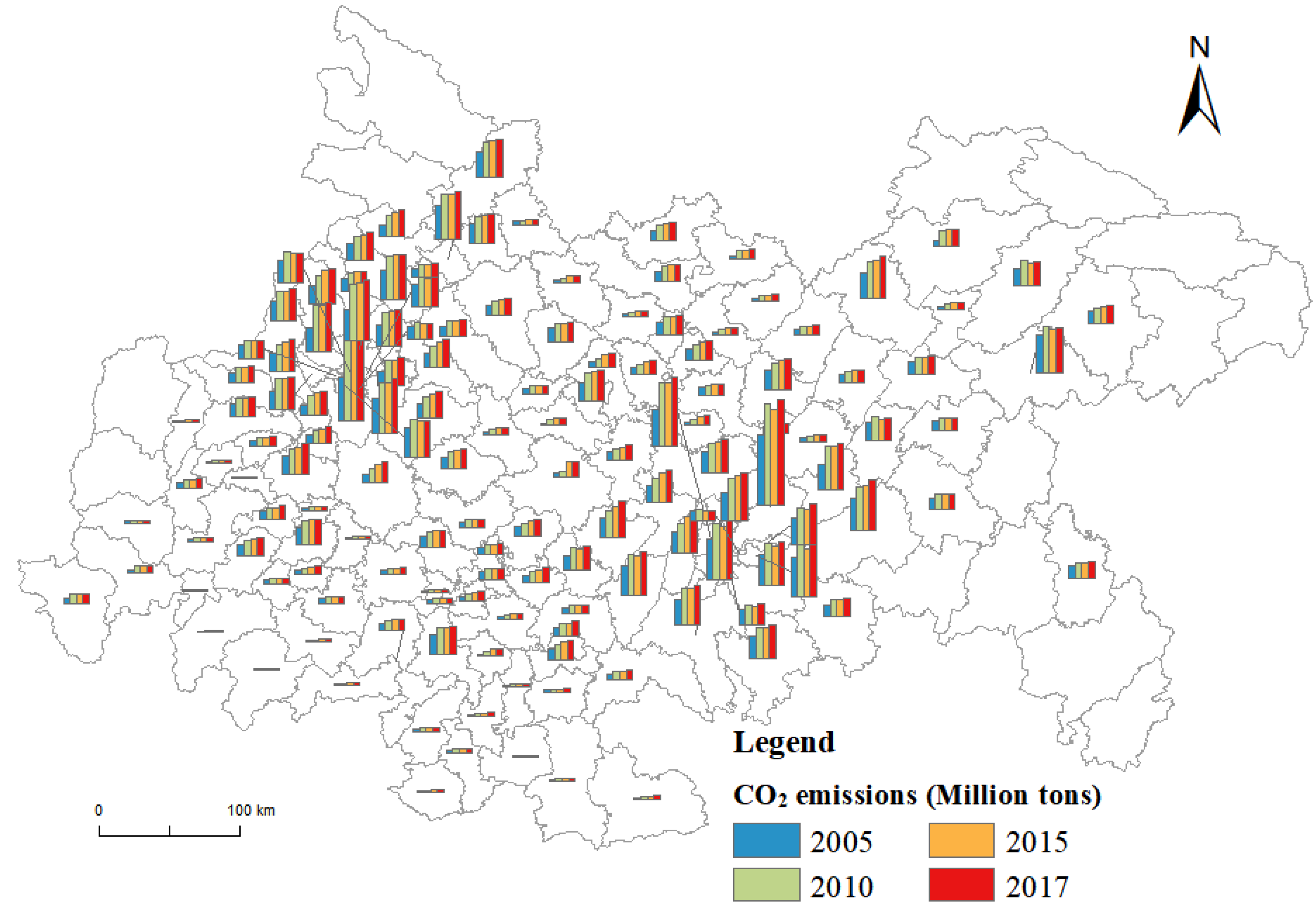
3.1.1. Spatial and Temporal Distribution Patterns of Carbon Emissions
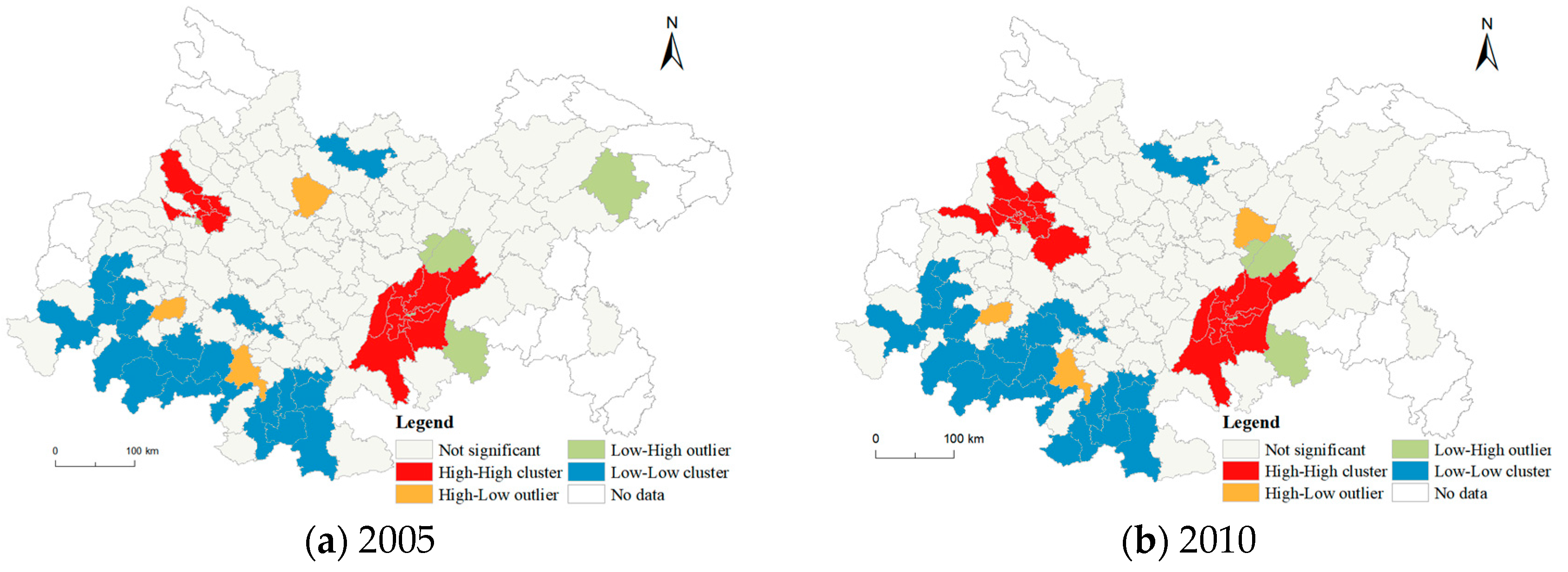
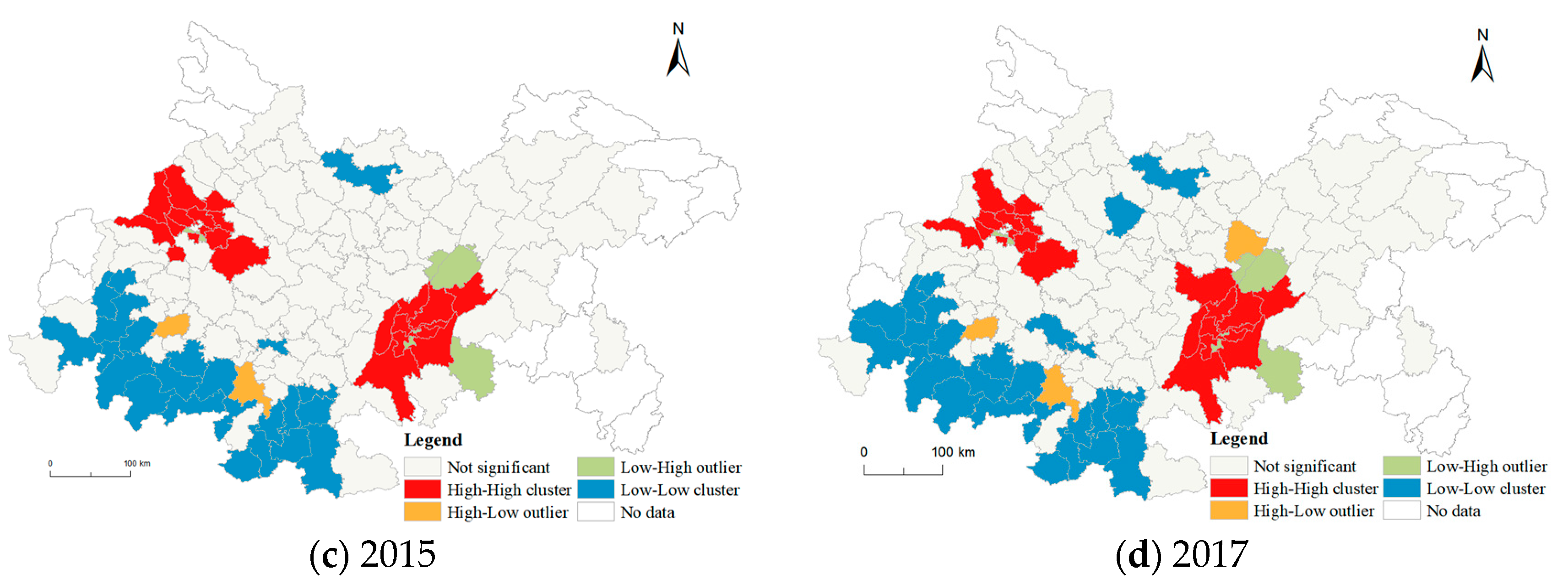
3.1.2. Spatial Autocorrelation Analysis
- (i).
- Global Autocorrelation Analysis
- (ii).
- Local Autocorrelation Analysis
3.2. Factors Influencing County-Level Carbon Emissions in the Chengdu–Chongqing Region
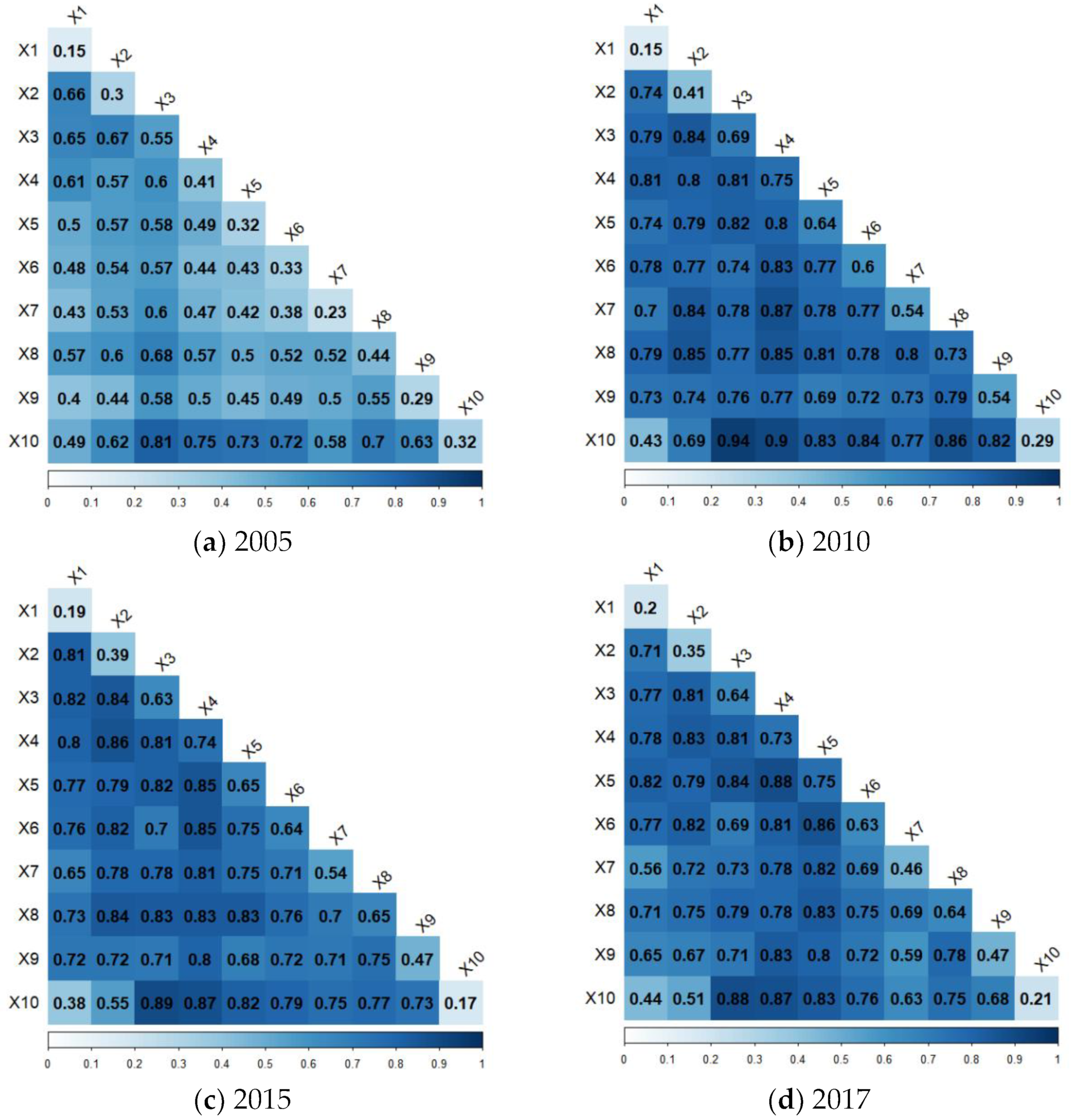
3.2.1. Temporal Variation of the Influencing Factors
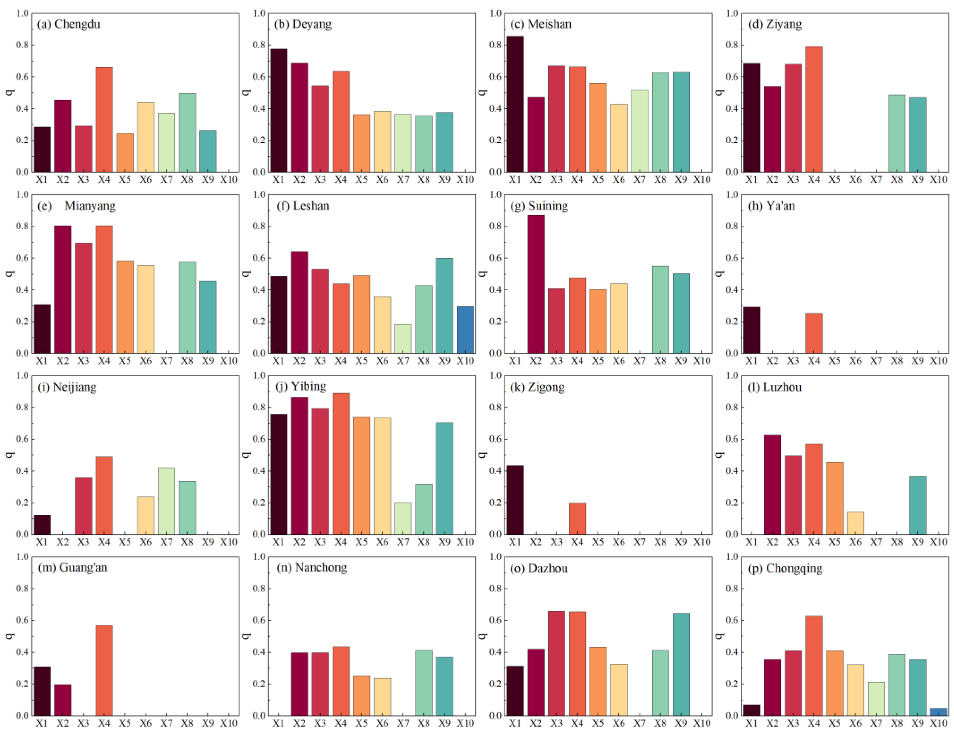
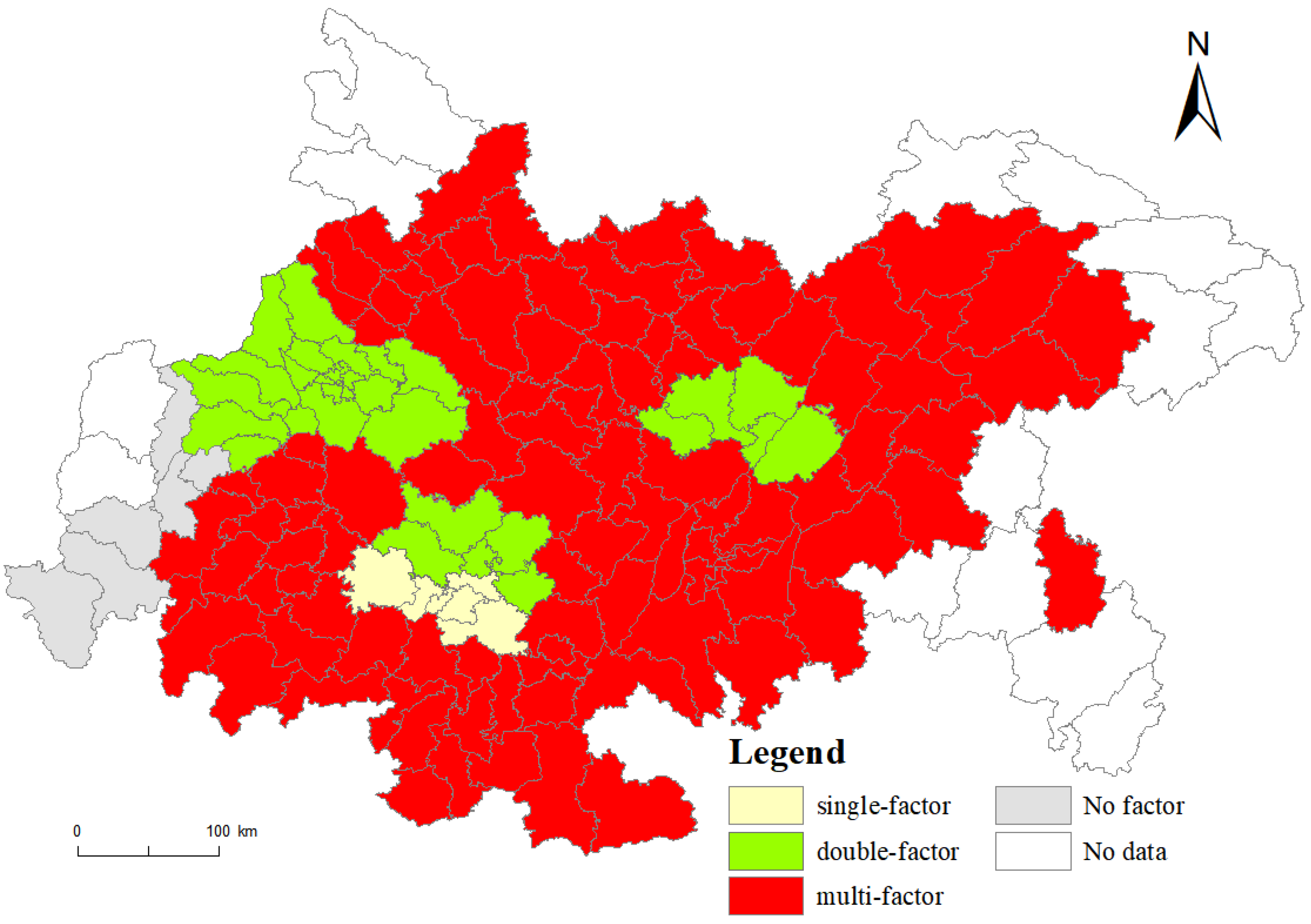
3.2.2. Regional Differences in the Influencing Factors
- (1)
- Population size influence type: The regions with strong X1 influence on carbon emissions include Meishan (0.86), Deyang (0.78), Yibin (0.76), Ziyang (0.69), Leshan (0.49), Zigong (0.44), Dazhou (0.31), Guang ‘an (0.31), Mianyang (0.31) and nine other cities.
- (2)
- Influence type of urbanization rate: The regions where carbon emissions are greatly affected by X2 include Suining (0.87), Yibin (0.87), Mianyang (0.81), Deyang (0.69), Leshan (0.64), Luzhou (0.63), Ziyang (0.54), Meishan (0.47), Chengdu (0.45), Dazhou (0.42), Nanchong (0.40), Chongqing (0.35) and another 12 cities.
- (3)
- Economic development influence type: The regions where carbon emissions are heavily affected by X3 include 12 cities, Yibin (0.80), Mianyang (0.70), Ziyang (0.68), Meishan (0.67), Dazhou (0.66), Deyang (0.55), Leshan (0.53), Luzhou (0.50), Suining (0.41), Chongqing (0.41), Nanchong (0.40) and Neijiang (0.36).
- (4)
- Industrial structure influence type: The regions where carbon emissions are strongly influenced by X4 include Yibin (0.89), Mianyang (0.81), Ziyang (0.79), Meishan (0.66), Chengdu (0.66), Dazhou (0.66), Deyang (0.64), Chongqing (0.63), Guang’an (0.57), Luzhou (0.57), Neijiang (0.49), Suining (0.48), Leshan (0.44), South Chong (0.44) and another 14 cities.
4. Discussion
4.1. Spatial and Temporal Distribution of Carbon Emissions
4.2. Factors Influencing County-Level Carbon Emissions
4.3. Limitations
- (1)
- Due to the difficulty of data acquisition at the county level, the impact factor indexes selected in this paper are not comprehensive and accurate. For example, energy utilization data at the county level is lacking, and energy-consumption-related indexes have not been considered. Technological progress should be represented by additional or comprehensive indicators such as the number of patents. Future research can be combined with regional development status, expand data collection sources, advance screen impact factors and update part of the data set to improve the timeliness of the research.
- (2)
- The geographical detector model is based on the analysis of spatial variance, and the continuous independent variables need to be discussed and converted into classification variables. The classification methods commonly used include equidistant segmentation, natural segmentation, quantile segmentation, geometric segmentation and standard deviation segmentation. This study discretized each influence factor according to the natural breakpoint method of conformity selection, which is characterized by making the difference between different types as large as possible. However, the results of the spatial discretization of continuous variables are related to the distillation method [34,63], and arbitrary zoning methods may mislead the actual relationship between geographical phenomena and their influence factors. Future research will also consider the regeneration effect, compare and analyze different discrete methods such as the natural breakpoint method, equidistant breakpoint method and quantile method, and also select the best personalization method suitable for the analysis of carbon emission impact factors in the Chengdu–Chongqing region.
5. Conclusions
- (i)
- Carbon emissions generally showed an annual growth trend of “first fast and then slow” with 2010 as the boundary. The average carbon emissions of the counties increased from 172 million tons to 283 million tons, with an annual growth rate of 4.24%. In terms of spatial distribution, the main urban areas of Chengdu and Chongqing show a circular pattern, in which the main urban areas of Chengdu and Chongqing are high-carbon-emission areas, the southern districts and counties are low-carbon-emission areas, and the central and northern regions are transition zones between high-carbon-emission areas and low-emission areas. Therefore, the economically developed areas and counties such as the main urban areas of Chengdu and Chongqing, as the key areas of carbon reduction, drive the surrounding areas and counties to gradually seek the path of low-carbon development to narrow the economic and social gap with the developed areas, so as to achieve the overall emission reduction target.
- (ii)
- Carbon emissions showed a significant spatial positive autocorrelation, the adjacent districts and counties mostly presented the spatial agglomeration characteristics of “high-high” or “low-low”, the number of high-high and low-low aggregation districts and counties was increasing, gradually spreading to the surrounding districts and counties, and the agglomeration state had a trend of strengthening. Therefore, high-carbon-emission areas such as the main urban areas of Chengdu and Chongqing should give full play to the coordination and spillover effect between neighboring districts and counties to carry out co-reduction and co-governance. Low-carbon-emission areas such as Ya ‘an City, Meishan City, Leshan City, Neijiang City, Zigong City, Yibin City and Luzhou City can learn from each other and demonstrate together.
- (iii)
- The influencing factors of carbon emission change significantly over time, and the influence of single factors is as follows in descending order: industrial structure > economic development > investment level > financial situation > social consumption > urbanization rate > technological progress > population size. The influence of the interaction factors was significantly higher than that of the single factor. However, the change trends of the influence of the single factor and the interaction factor were similar, and most of them had a trend of increasing first and then decreasing. Therefore, the key to realize the overall carbon emission reduction is to make full use of the regional social economy and resource endowment, give play to the advantages of late development, rationally regulate social and economic factors, and take the low-carbon and circular development road with the characteristics of the Chengdu–Chongqing region.
- (iv)
- There are obvious regional differences in the influencing factors of carbon emissions. County carbon emissions of 9 cities, such as Meishan, are of the population size influencing type; the district and county carbon emissions of 12 cities, such as Suining, Yibin and Mianyang, are of the urbanization rate influencing type; the district and county carbon emissions of 12 cities, such as Yibin, are of the economic development influencing type. Yibin City, Mianyang City and another 14 cities are affected by the industrial structure, showing a two-factor influence as the core, and the county carbon emission in the Chengdu–Chongqing region is affected by multiple factors. Therefore, the formulation and implementation of carbon emission reduction policies should consider the stage differences of regional development, pay attention to the mutual integration of various influence factors, and promote resource integration, so as to achieve regional carbon emission reductions.
Author Contributions
Funding
Institutional Review Board Statement
Informed Consent Statement
Data Availability Statement
Conflicts of Interest
References
- Hu, X.; Zhang, Z.; Chen, X.; Wang, Y. Geographical detection of spatial and temporal differences and influencing factors of county economic development--Gansu Province as an example. Geogr. Res. 2019, 38, 772–783. [Google Scholar] [CrossRef]
- Wang, R.; Zhang, H.; Feng, L. Impact of China’s county scale and structure on household carbon emissions: Key elements and representative indicators. Mod. Urban Res. 2021, 36, 126–132. [Google Scholar] [CrossRef]
- Sun, Y.; Zheng, S.; Wu, Y.; Schlink, U.; Singh, R. Spatiotemporal variations of city-level carbon emissions in China during 2000-2017 using nighttime light data. Remote Sens. 2020, 12, 2916. [Google Scholar] [CrossRef]
- Chen, L.; Xu, L.; Cai, Y.; Yang, Z. Spatiotemporal patterns of industrial carbon emissions at the city level. Resour. Conserv. Recycl. 2021, 169, 105499. [Google Scholar] [CrossRef]
- Cantore, N.; Padilla, E. Equality and CO2 emissions distribution in climate change integrated assessment modeling. Energy 2010, 35, 298–313. [Google Scholar] [CrossRef]
- Clarke-Sather, A.; Qu, J.; Wang, Q.; Zeng, J.; Li, Y. Carbon inequality at the sub-national scale: A case study of provincial-level inequality in CO2 emissions in China 1997–2007. Energy Policy 2011, 39, 5420–5428. [Google Scholar] [CrossRef]
- Mussini, M.; Grossi, L. Decomposing changes in CO2 emission inequality overtime: The roles of re-ranking and changes in per capita CO2 emission disparities. Energy Econ. 2015, 49, 274–281. [Google Scholar] [CrossRef]
- Liu, H.; Shao, M.; Ji, Y. The spatial pattern and distribution dynamic evolution of carbon emissions in China: Empirical study based on county carbon emission data. Sci. Geogr. Sin. 2021, 41, 1917–1924. [Google Scholar] [CrossRef]
- Wang, S.; Fang, C.; Wang, Y. Spatiotemporal variations of energy-related CO2 emissions in China and its influencing factors: An empirical analysis based on provincial panel data. Renew. Sustain. Energy Rev. 2016, 55, 505–515. [Google Scholar] [CrossRef]
- Liu, X.; Guo, R.; Zhang, Y.; Zhang, D.; Wang, Z.; Gao, C.; Xie, J. Nonparametric estimation and empirical analysis of spatial dependence structure of provincial carbon emissions in China. China Popul. Resour. Environ. 2019, 29, 40–51. [Google Scholar]
- Wang, S.; Huang, Y. Spatial spillover effect and driving forces of carbon emission intensity at city level in China. Acta Geogr. Sin. 2019, 74, 1131–1148. [Google Scholar] [CrossRef]
- Wang, Y.; He, Y. Spatial and temporal patterns and influencing factors of provincial CO2 emissions in China. World Geogr. Res. 2020, 29, 512–522. [Google Scholar] [CrossRef]
- Liu, Q.; Wu, S.; Lei, Y. Exploring spatial characteristics of city-level CO2 emissions in China and their influencing factors from global and local perspectives. Sci. Total Environ. 2021, 754, 142206. [Google Scholar] [CrossRef]
- Shen, L.; Wu, Y.; Lou, Y.; Zeng, D.; Shuai, C.; Song, X. What drives the carbon emission in the Chinese cities? A case of pilot low carbon city of Beijing. J. Clean. Prod. 2018, 174, 343–354. [Google Scholar] [CrossRef]
- Xu, S.; He, Z.; Long, R. Factors that influence carbon emissions due to energy consumption in China: Decomposition analysis using LMDI. Appl. Energy 2014, 127, 182–193. [Google Scholar] [CrossRef]
- Shuai, C.; Shen, L.; Jiao, L.; Wu, Y.; Tan, Y. Identifying key impact factors on carbon emission: Evidences from panel and time-series data of 125 countries from 1990 to 2011. Appl. Energy 2017, 187, 310–325. [Google Scholar] [CrossRef]
- Bai, Y.; Deng, X.; Gibson, J.; Zhao, Z.; Xu, H. How does urbanization affect residential CO2 emissions? An analysis on urban agglomerations of China. J. Clean. Prod. 2019, 209, 876–885. [Google Scholar] [CrossRef]
- Guo, L.; Ning, C.; Wang, W. Measurement and effect decomposition of carbon emissions on the production side of forest products in China--based on a multi-regional input-output and structural decomposition analysis model. For. Econ. 2022, 44, 23–40. [Google Scholar] [CrossRef]
- Sun, J.; Liu, Y.; Zhao, R.; Yang, W.; Wu, H.; Peng, C.; Guo, M.; Liu, K. Input-output based water-soil-carbon footprint flow analysis of inter-provincial agriculture in China. J. Ecol. 2022, 42, 9615–9626. [Google Scholar] [CrossRef]
- Wang, Z.; Li, Z.; Wu, W. Spatial and temporal evolution of carbon emissions in different classes of cities in the Yangtze River Economic Belt and its influencing factors. Environ. Sci. Res. 2022, 35, 2273–2281. [Google Scholar] [CrossRef]
- Zhou, C.; Wang, S. Examining the determinants and the spatial nexus of city-level CO2 emissions in China: A dynamic spatial panel analysis of China’s cities. J. Clean. Prod. 2018, 171, 917–926. [Google Scholar] [CrossRef]
- Wang, S.; Liu, X.; Zhou, C.; Hu, J.; Ou, J. Examining the impacts of socioeconomic factors, urban form, and transportation networks on CO2 emissions in China’s megacities. Appl. Energy 2017, 185, 189–200. [Google Scholar] [CrossRef]
- Li, A.; Zhang, A.; Zhou, Y.; Yao, X. Decomposition analysis of factors affecting carbon dioxide emissions across provinces in China. J. Clean. Prod. 2017, 141, 1428–1444. [Google Scholar] [CrossRef]
- Lioboikiene, G.; Butkus, M. Scale, composition, and technique effects through which the economic growth, foreign direct investment, urbanization, and trade affect greenhouse gas emissions. Renew. Energy 2019, 132, 13101322. [Google Scholar] [CrossRef]
- Feng, D.; Li, J. Impacts of urbanization on carbon dioxide emissions in the three urban agglomerations of China. Resour. Environ. Yangtze Basin 2018, 27, 2194–2200. [Google Scholar]
- Wang, F.; Ga, M.; Liu, J.; Qin, Y.; Wang, G.; Fan, W.; Ji, L. An empirical study on the impact path of urbanization to carbon emissions in the China Yangtze River Delta urban agglomeration. Appl. Sci. 2019, 9, 11166. [Google Scholar] [CrossRef] [Green Version]
- Wang, Q.; Su, M. The effects of urbanization and industrialization on decoupling economic growth from carbon emission—A case study of China. Sustain. Cities Soc. 2019, 51, 101758. [Google Scholar] [CrossRef]
- Wang, S.; Su, Y.; Zhao, Y. Regional inequality, spatial spillover effects and influencing factors of China’s city-level energy-related carbon emissions. Acta Geogr. Sin. 2018, 73, 414–428. [Google Scholar] [CrossRef]
- Wang, S.; Liu, Y.; Fang, C. Review of energy-related CO2 emission in response to climate change. Prog. Geogr. 2015, 34, 151–164. [Google Scholar] [CrossRef]
- Fan, J.; Zhou, L. The mechanism and effect of urbanization and real estate investment on carbon emissions in China. Sci. Geogr. Sin. 2019, 39, 644–653. [Google Scholar] [CrossRef]
- Wang, J.; Xu, C. Geographic detectors: Principles and perspectives. J. Geogr. 2017, 72, 116–134. [Google Scholar] [CrossRef]
- Liao, Y.; Zhang, Y.; He, L.; Wang, J.; Liu, X.; Zhang, N.; Xu, B. Temporal and spatial analysis of neural tube defects and detection of geographical factors in Shanxi Province, China. PLoS ONE 2016, 11, e0150332. [Google Scholar] [CrossRef]
- Shen, J.; Zhang, N.; Gexigeduren; He, B.; Liu, C.; Li, Y.; Zhang, H.; Chen, X.; Lin, H. Construction of a GeogDetector-based model system to indicate the potential occurrence of grasshoppers in Inner Mongolia steppe habitats. Bulletin of Entomological. Bull. Entomol. Res. 2015, 105, 335–346. [Google Scholar] [CrossRef] [Green Version]
- Ju, H.; Zhang, Z.; Zuo, L.; Wang, J.; Zhang, S.; Wang, X.; Zhao, X. Driving forces and their interactions of built-up land expansion based on the geographical detector: A case study of Beijing, China. Int. J. Geogr. Inf. Sci. 2016, 30, 2188–2207. [Google Scholar] [CrossRef]
- Wang, S.; Wang, Y.; Lin, X.; Zhang, H. Spatial differentiation patterns and influencing mechanism of housing prices in China: Based on data of 2872 counties. Acta Geogr. Sin. 2016, 71, 1329–1342. [Google Scholar] [CrossRef]
- Zhou, L.; Wu, J.; Jia, R.; Liang, N. Investigation of temporal-spatial characteristics and underlying risk factors of PM2.5 pollution in Beijing-Tianjin-Hebei Area. Res. Environ. Sci. 2016, 29, 483–493. [Google Scholar] [CrossRef]
- Wu, R.; Zhang, J.; Bao, Y.; Zhang, F. Geographical detector model for influencing factors of industrial sector carbon dioxide emissions in Inner Mongolia, China. Sustainability 2016, 8, 149. [Google Scholar] [CrossRef] [Green Version]
- Cao, J.; Zhou, L. Study on the spatial and temporal distribution of carbon emissions from logistics industry in Yangtze River Delta region and its influencing factors. Stat. Decis. Mak. 2021, 37, 79–83. [Google Scholar] [CrossRef]
- Lin, X.; Bian, Y.; Wang, D. Spatial and temporal evolution characteristics and influencing factors of industrial carbon emission efficiency in Beijing-Tianjin-Hebei region. Econ. Geogr. 2021, 41, 187–195. [Google Scholar] [CrossRef]
- Li, A.; Wang, Y.; Li, M.; Wang, B.; Chen, W. Structural characteristics and influencing factors of spatially linked networks of carbon emissions: A case study of three major urban agglomerations in China. Environ. Sci. Technol. 2021, 44, 186–193. [Google Scholar] [CrossRef]
- Huang, B.; Meng, L. Convergence of per capita carbon dioxide emissions in urban China: A spatio-temporal perspective. Appl. Geogr. 2013, 40, 21–29. [Google Scholar] [CrossRef]
- Wang, S.; Xie., Z.; Wang, Z. Spatial and temporal evolution of carbon emissions in Chinese counties and the influencing factors. J. Geogr. 2021, 76, 3103–3118. [Google Scholar]
- Sun, G.; Wang, C. Research on Dynamic Changes of Land Use and Landscape Pattern in Chengdu-Chongqing Economic Circle. Agric. Sci. 2022, 50, 59–63. [Google Scholar] [CrossRef]
- Zeng, H.; Shao, B.; Bian, G.; Dai, H.; Zhou, F. Analysis of Influencing Factors and Trend Forecast of CO2 Emission in Chengdu-Chongqing Urban Agglomeration. Sustainability 2022, 14, 1167. [Google Scholar] [CrossRef]
- Tille, Y.; Dickson, M.M.; Espa, G.; Giuliani, D. Measuring the spatial balance of a sample: A new measure based on Moran’s I index. Spat. Stat. 2018, 23, 182–192. [Google Scholar] [CrossRef] [Green Version]
- Anselin, L. Local Indicators of Spatial association-LISA. Geogr. Anal. 1995, 27, 93–115. [Google Scholar]
- Wang, J.; Li, X.; Christakos, G.; Liao, Y.; Zhang, T.; Gu, X.; Zheng, X. Geographical detectors-based health risk assessment and its application in the neural tube defects study of the Heshun region, China. Int. J. Geogr. Inf. Sci. 2010, 24, 107–127. [Google Scholar] [CrossRef]
- Wang, J.; Hu, Y. Environmental health risk detection with GeogDetector. Environ. Model. Softw. 2012, 33, 114–115. [Google Scholar] [CrossRef]
- Chen, G.; Luo, J.; Zhang, C.; Jiang, L.; Tian, L.; Chen, G. Characteristics and influencing factors of spatial differentiation of urban black and odorous waters in China. Sustainability 2018, 10, 4747. [Google Scholar] [CrossRef] [Green Version]
- Spatial Analysis Group, IGSNRR, 2013. Excel-GeoDetector. Chinese Academy of Sciences. Available online: http://www.sssampling.org/Excel-Geodetector/ (accessed on 10 October 2015).
- Wang, H.; Chen, C.; Pan, T.; Liu, C.; Chen, L.; Sun, L. County scale characteristics of CO2 emission’s spatial-temporal evolution in the Beijing-TianjinHebei metropolitan region. Environ. Sci. 2014, 35, 385–393. [Google Scholar]
- Peng, W.; Zhou, J.; Xu, X.; Luo, H.; Zhao, J.; Yang, C. Effect of land use changes on carbon emission and its spatial patterns in Chengdu Plain and its surrounding area, western China, from 1990 to 2010. Ecol. Sci. 2017, 36, 105–114. [Google Scholar] [CrossRef]
- Sun, X.; Shi, K.; Wu, J. Spatiotemporal dynamics of CO2 emissions in Chongqing: An empirical analysis at the county level. Environ. Sci. 2018, 39, 2971–2981. [Google Scholar]
- Wang, R.; Zhang, H.; Qiang, W.; Li, F.; Peng, J. Spatial characteristics and influencing factors of carbon emissions in county-level cities of China based on urbanization. Prog. Geogr. 2021, 40, 1999–2010. [Google Scholar] [CrossRef]
- Han, C.; Song, F.; Teng, M. Temporal and spatial dynamic characteristics, spatial clustering and governance strategies of carbon emissions in the Yangtze River. Delta 2022, 36, 24–33. [Google Scholar] [CrossRef]
- Wei, F.; Wei, Y.; Tong, X. Spatio-temporal evolution characteristics and driving factors of carbon emissions in Dongrong development area of Eastern Guangxi Zhuang Autonomous Region. Bull. Soil Water Conserv. 2022, 42, 381–389. [Google Scholar]
- Xu, J.; Pan, H.; Cao, X.; Zhao, X. County carbon emission effect of Meishan City based on LUCC. J. Sichuan Norm. Univ. 2020, 43, 683–689. [Google Scholar] [CrossRef]
- Zhao, W.; Luo, S.; Yuan, X.; Zhang, Q.; Yang, F.; Liu, Y.; Xie, W. Spatiotemporal pattern and influencing factors of carbon emissions at county level in Shanxi Province. Environ. Sci. Technol. 2022, 45, 226–236. [Google Scholar] [CrossRef]
- Li, J.; Huang, X.; Wu, C.; Zhou, Y.; Xu, G. Analysis of Spatial Heterogeneity Impact Factors on Carbon Emissions in China. Econ. Geogr. 2015, 35, 21–28. [Google Scholar] [CrossRef]
- Yu, W.; Zhang, T.; Shen, D. County-level spatial pattern and influencing factors evolution of carbon emission intensity in China: A random forest model analysis. China Environ. Sci. 2022, 42, 2788–2798. [Google Scholar] [CrossRef]
- Wang, S.; Xie, Z.; Wang, Z. The spatiotemporal pattern evolution and influencing factors of CO2 emissions at the county level of China. Acta Geogr. Sin. 2021, 76, 3103–3118. [Google Scholar] [CrossRef]
- Zhang, H.; Yuan, P.; Zhu, Z. City population size, industrial agglomeration and CO2 emission in Chinese prefectures. China Environ. Sci. 2021, 41, 2459–2470. [Google Scholar] [CrossRef]
- Cao, F.; Ge, Y.; Wang, J. Optimal discretization for geographical detectors-based risk assessment. GISci. Remote Sens. 2013, 50, 78–92. [Google Scholar] [CrossRef]


| Name | High-High Clustering | High-Low Clustering | Low-High Clustering | Low-Low Clustering |
|---|---|---|---|---|
| Correlation judgment | Space-positive correlation | Space-negative correlation | Space-positive correlation | Space-negative correlation |
| Aggregation mode | High values surrounded by high values | High values surrounded by low values | Low values surrounded by high values | Low values surrounded by low values |
| Description | Interaction |
|---|---|
| q(x1∩x2) < Min(q(x1), q(x2)) | Weakening, nonlinear |
| Min(q(x1), q(x2)) < q(x1∩x2) < Max(q(x1), q(x2)) | Weakened, unique |
| q(x1∩x2) > Max(q(x1), q(x2)) | Enhanced, bilinear |
| q(x1∩x2) = q(x1) + q(x2) | Independent |
| q(x1∩x2) > q(x1) + q(x2) | Enhanced, nonlinear |
| Variables | Indicator Description | Unit | AVG | SD | Min | Max |
|---|---|---|---|---|---|---|
| Carbon emissions | Total carbon emissions (Y) | Million tons | 2.47 | 2.22 | 0.08 | 14.75 |
| Population size | Year-end population (X1) | 10000 persons | 72.48 | 37.80 | 4.99 | 181.30 |
| Urban rate | Proportion of urban population to total population (X2) | % | 33.59 | 22.96 | 5.52 | 100.00 |
| Economic development | Gross domestic product (X3) | 100 million CNY | 194.40 | 197.63 | 6.94 | 1447.20 |
| Industrial structure | Scale of output value of secondary industry (X4) | 95.49 | 101.70 | 1.91 | 926.84 | |
| Scale of output value of tertiary industry (X5) | 77.06 | 119.97 | 1.06 | 1089.88 | ||
| Financial situation | General public budget revenue (X6) | 10.89 | 14.83 | 0.15 | 113.49 | |
| General public budget expenditure (X7) | 25.87 | 22.51 | 0.97 | 14.99 | ||
| Investment level | Total social fixed asset investment (X8) | 150.50 | 159.92 | 1.49 | 1248.22 | |
| Social consumption | Total retail sales of consumer goods (X9) | 80.81 | 112.73 | 1.10 | 956.29 | |
| Technological progress | Carbon emission intensity (X10) | Tons/10000 CNY | 1.55 | 0.98 | 0.03 | 6.72 |
| Year | 2005 | 2010 | 2015 | 2017 |
|---|---|---|---|---|
| Moran’s I | 0.446 | 0.459 | 0.460 | 0.463 |
| Z | 8.686 | 8.939 | 8.939 | 8.999 |
| P | 0.000 | 0.000 | 0.000 | 0.000 |
| Factors | 2005 | 2010 | 2015 | 2017 | Average |
|---|---|---|---|---|---|
| Scale of output value of secondary industry (X4) | 3 (0.41) | 1 (0.75) | 1 (0.74) | 2 (0.73) | 1 (0.66) |
| Gross domestic product (X3) | 1 (0.55) | 3 (0.69) | 5 (0.63) | 4 (0.64) | 2 (0.63) |
| Total social fixed asset investment (X8) | 2 (0.44) | 2 (0.73) | 3 (0.65) | 3 (0.64) | 3 (0.61) |
| Scale of output value of tertiary industry (X5) | 5 (0.32) | 4 (0.64) | 2 (0.65) | 1 (0.75) | 4 (0.59) |
| General public budget revenue (X6) | 4 (0.32) | 5 (0.60) | 4 (0.64) | 5 (0.63) | 5 (0.55) |
| General public budget expenditure (X7) | 9 (0.23) | 7 (0.54) | 6 (0.54) | 7 (0.46) | 6 (0.44) |
| Total retail sales of consumer goods (X9) | 8 (0.29) | 6 (0.54) | 7 (0.47) | 6 (0.47) | 7 (0.44) |
| Proportion of urban population to total population (X2) | 7 (0.30) | 8 (0.41) | 8 (0.39) | 8 (0.35) | 8 (0.36) |
| Carbon emission intensity (X10) | 6 (0.32) | 9 (0.29) | 9 (0.16) | 9 (0.21) | 9 (0.25) |
| Year-end population (X1) | 10 (0.15) | 10 (0.15) | 10 (0.19) | 10 (0.20) | 10 (0.17) |
Disclaimer/Publisher’s Note: The statements, opinions and data contained in all publications are solely those of the individual author(s) and contributor(s) and not of MDPI and/or the editor(s). MDPI and/or the editor(s) disclaim responsibility for any injury to people or property resulting from any ideas, methods, instructions or products referred to in the content. |
© 2023 by the authors. Licensee MDPI, Basel, Switzerland. This article is an open access article distributed under the terms and conditions of the Creative Commons Attribution (CC BY) license (https://creativecommons.org/licenses/by/4.0/).
Share and Cite
Chen, X.; Qin, J.; Yao, J.; Yang, Z.; Li, X. The Distribution and Impact Characteristics of Small-Scale Carbon Emissions in the Chengdu–Chongqing Region. Atmosphere 2023, 14, 216. https://doi.org/10.3390/atmos14020216
Chen X, Qin J, Yao J, Yang Z, Li X. The Distribution and Impact Characteristics of Small-Scale Carbon Emissions in the Chengdu–Chongqing Region. Atmosphere. 2023; 14(2):216. https://doi.org/10.3390/atmos14020216
Chicago/Turabian StyleChen, Xin, Jialing Qin, Jian Yao, Zhishan Yang, and Xuedong Li. 2023. "The Distribution and Impact Characteristics of Small-Scale Carbon Emissions in the Chengdu–Chongqing Region" Atmosphere 14, no. 2: 216. https://doi.org/10.3390/atmos14020216