Tropical Cyclone Detection from the Thermal Infrared Sensor IASI Data Using the Deep Learning Model YOLOv3

Abstract

Tropical cyclone (TC) detection is essential to mitigate natural disasters, as TCs can cause significant damage to life, infrastructure and economy. In this study, we applied the deep learning object detection model YOLOv3 to detect TCs in the North Atlantic Basin, using data from the Thermal InfraRed (TIR) Atmospheric Sounding Interferometer (IASI) onboard the Metop satellites. IASI measures the outgoing TIR radiation of the Earth-Atmosphere. For the first time, we provide a proof of concept of the possibility of constructing images required by YOLOv3 from a TIR remote sensor that is not an imager. We constructed a dataset by selecting 50 IASI radiance channels and using them to create images, which we labeled by constructing bounding boxes around TCs using the hurricane database HURDAT2. We trained the YOLOv3 on two settings, first with three “best” selected channels, then using an autoencoder to exploit all 50 channels. We assessed its performance with the Average Precision (AP) metric at two different intersection over union (IoU) thresholds (0.1 and 0.5). The model achieved promising results with AP at IoU threshold 0.1 of 78.31%. Lower performance was achieved with IoU threshold 0.5 (31.05%), showing the model lacks precision regarding the size and position of the predicted boxes. Despite that, we show YOLOv3 demonstrates great potential for TC detection using TIR instruments data.

1. Introduction

A tropical cyclone (TC) is a large-scale air mass that rotates around a strong center of low atmospheric pressure, accompanied by intense variation in physical variables such as temperature, wind speed, and pressure, inducing events such as heavy rain, storm surges, flooding, etc. [1]. It is characterized by a warm core and circular wind motion around a well-defined center, clockwise in the southern hemisphere and anti-clockwise in the northern hemisphere. According to the Atlantic Oceanographic and Meteorological Laboratory from the National Oceanic and Atmospheric Administration (NOAA), if its maximum sustained wind is under 34 knots (about 63 km/h), it is called a tropical depression [1]. When the wind exceeds that threshold, it becomes a tropical storm. Once it exceeds 64 knots, it is classified as a hurricane. In this study, we focused on detecting TCs with maximum sustained wind of at least 34 knots (tropical storms and hurricanes). More explanation is provided in Section 2.3. Due to its destructive potency, human losses, physical and economic damages can be significant. It is, therefore, essential to be able to automatically detect TCs to mitigate their risk and potentially analyze their characteristics.

As the understanding of TC remains incomplete, predicting TC activity is a challenging task. Prevalent physical models for TC detection are near real-time two-stage detectors with spatial search and temporal correlation based on thresholded criteria using high-resolution climate data (vorticity, vertical temperatures, sea-level temperature and pressure) [2,3]. Such algorithms aim to identify and track TCs in gridded climate data or even in unstructured grids [4] and connect them into a trajectory. Bourdin et al. [5] intercompared four physical models on the European Centre for Medium-Range Weather Forecasts (ECMWF) Reanalysis 5th generation (ERA5). Such methodologies have been frequently used in the past decades [4] and show great ability, and potential in assessing TC activity [6,7]. With the enhancement of computational resources, high-resolution climate datasets have been growing increasingly. Studies demonstrate that the use in climate models of datasets with higher horizontal resolution shows great promise in improving the prediction of TCs [7,8]. The downside of this type of method is that they often require setting up a number of well-defined rules or thresholds. However, complex weather phenomena such as TCs remain difficult to quantify and predict [9].

A frequently used method is the CLImatology and PERsistence (CLIPER) model [10], used as a baseline in most statistical forecasting. It is based on linear regression and uses predictors related to climatology and persistence, such as current storm location, storm motion, maximum sustained wind speed, and previous storm motion. Later on, many studies proposed methods based on the CLIPER model [11,12].

With the emergence of machine learning (ML) and, more particularly, neural network (NN) applications, such methods can be effectively applied in the meteorological domain. The advantage of such techniques over more traditional ones is that ML does not require any assumption: in contrast with explicit models based on thresholded criteria, ML techniques implicitly learn from a given set of examples from real life to provide and resolve complex and ambiguous features [9]. It can, therefore, be advantageous to use NNs to detect complex weather systems such as TCs, which are difficult to describe and quantify. Deep learning (DL) models have the advantage of being able to process high quantities of data, which is a key point as huge volumes of data are being continuously generated by satellites, radar, or ground-based instruments. Shi et al. [13] used an object detection model named Single Shot Detector (SSD) to detect extratropical cyclones at different stages (developing, mature, and declining). For their part, Kumler-Bonfanti et al. [9] used deep learning image segmentation models using the U-Net architecture to segment images and identify the areas of tropical and extratropical cyclones. Input data contained data from current t, t − 1, and t− 2 time steps for the starting t time step, giving a sense of time and cyclone rotation to the model. Both approaches have been successful in detecting cyclones.

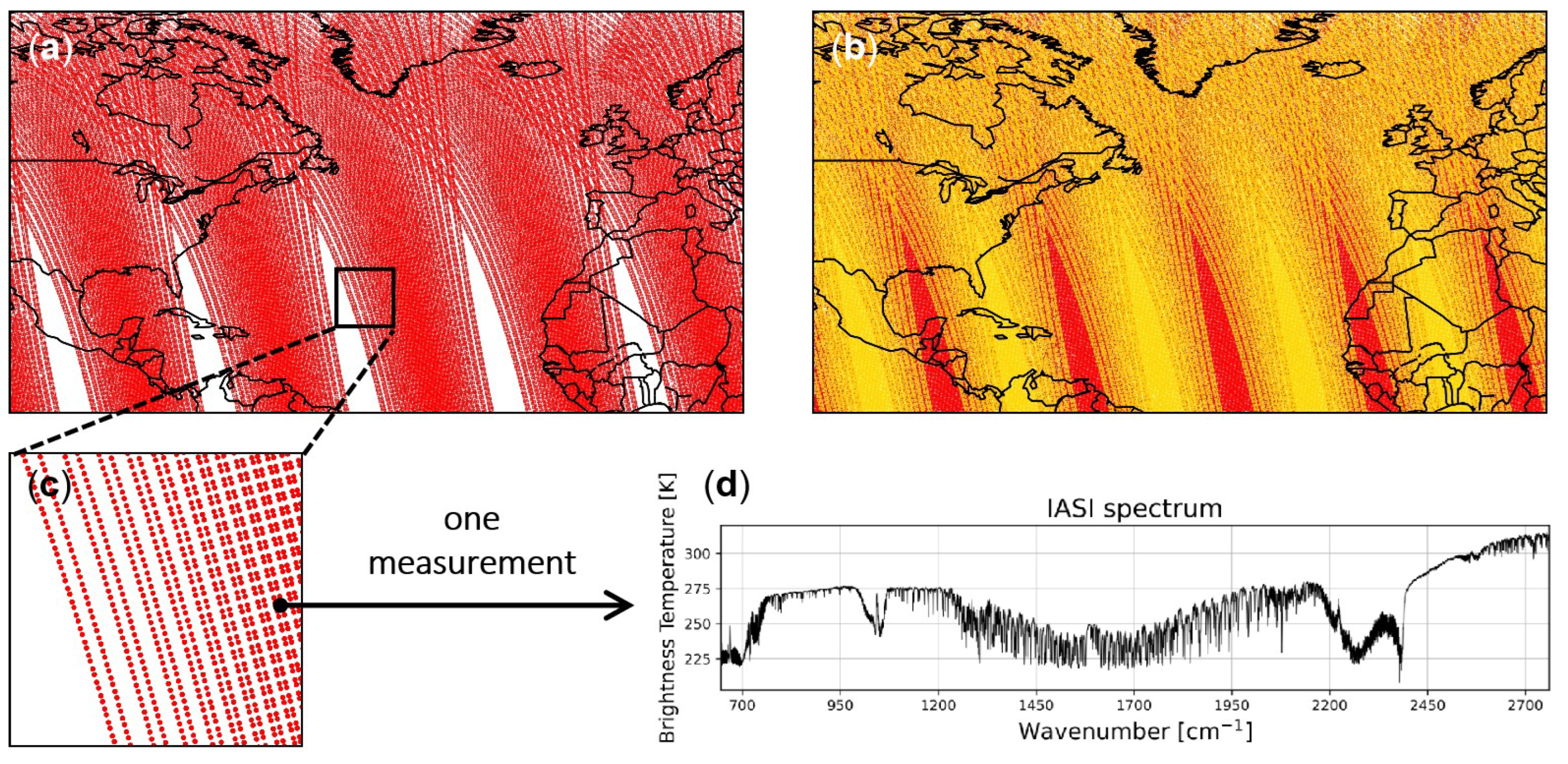
In this paper, we used data from the Infrared Atmospheric Sounding Interferometer (IASI) [14] on board the Metop satellites (more information on IASI is provided in Section 2.1). IASI is a passive remote sensor that measures the thermal infrared radiation (i.e., heat) as it exits land, through the atmosphere, and into space. It is, therefore, not the typical sensor/imager used to monitor cyclonic activity. However, it is largely used for numerical weather prediction [15] and to monitor the atmospheric composition [14,16]. Due to its excellent stability, IASI is a reference instrument that is used to calibrate other infrared sensors [17,18]. IASI radiance data is made available by the European Organisation for the Exploitation of Meteorological Satellites (EUMETSAT) dissemination system so that near real-time processing of the data is possible. More than 4 million IASI spectra covering the entire Earth are collected per day (17 Terabytes per year), from which a significant part (about 70%) is affected by the presence of clouds. Most of these cloud-contaminated data are discarded in retrieval processes of chemical species like CO, O${}_3$ or NH${}_3$ for instance [14,19]. Here we will exploit all the IASI data in an attempt to develop the value of these usually discarded cloudy data. No other instruments and no wind data are used.

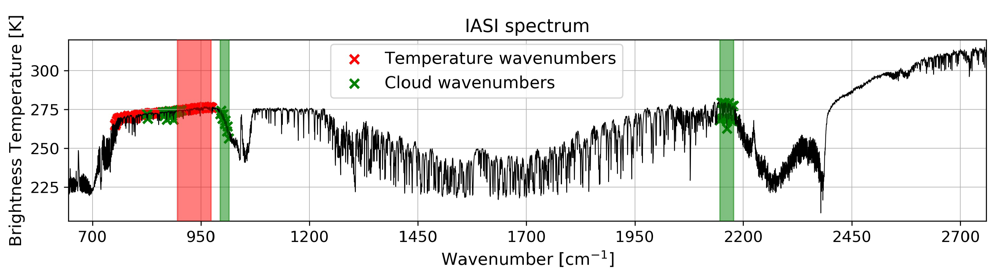
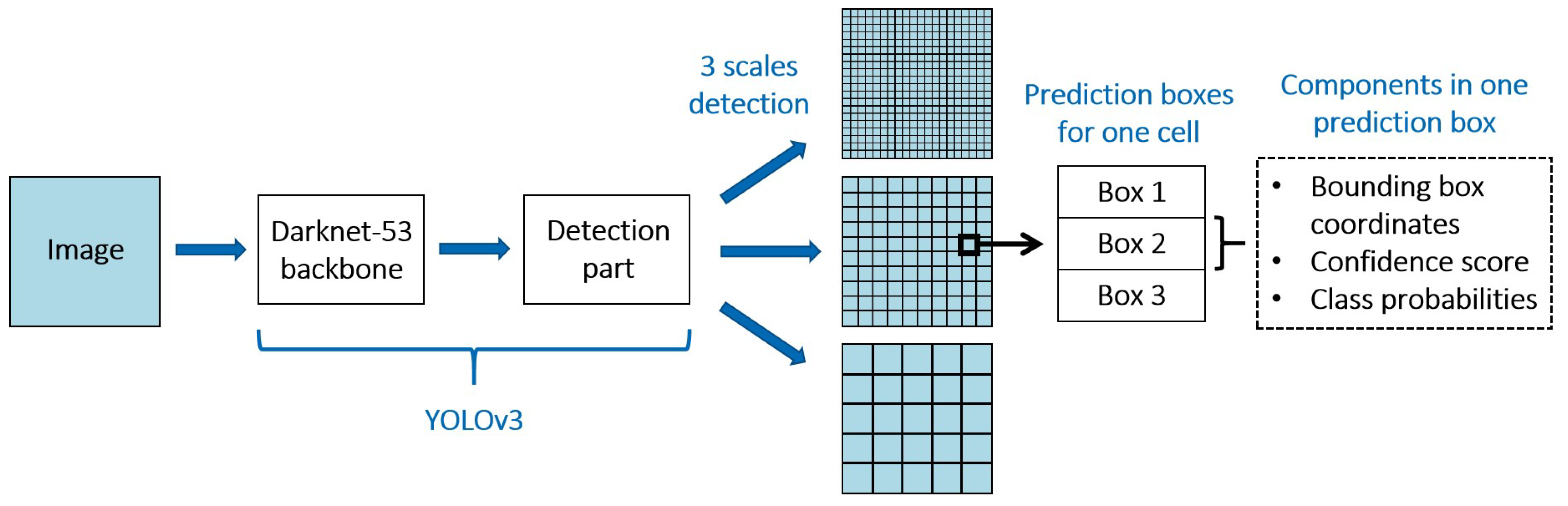
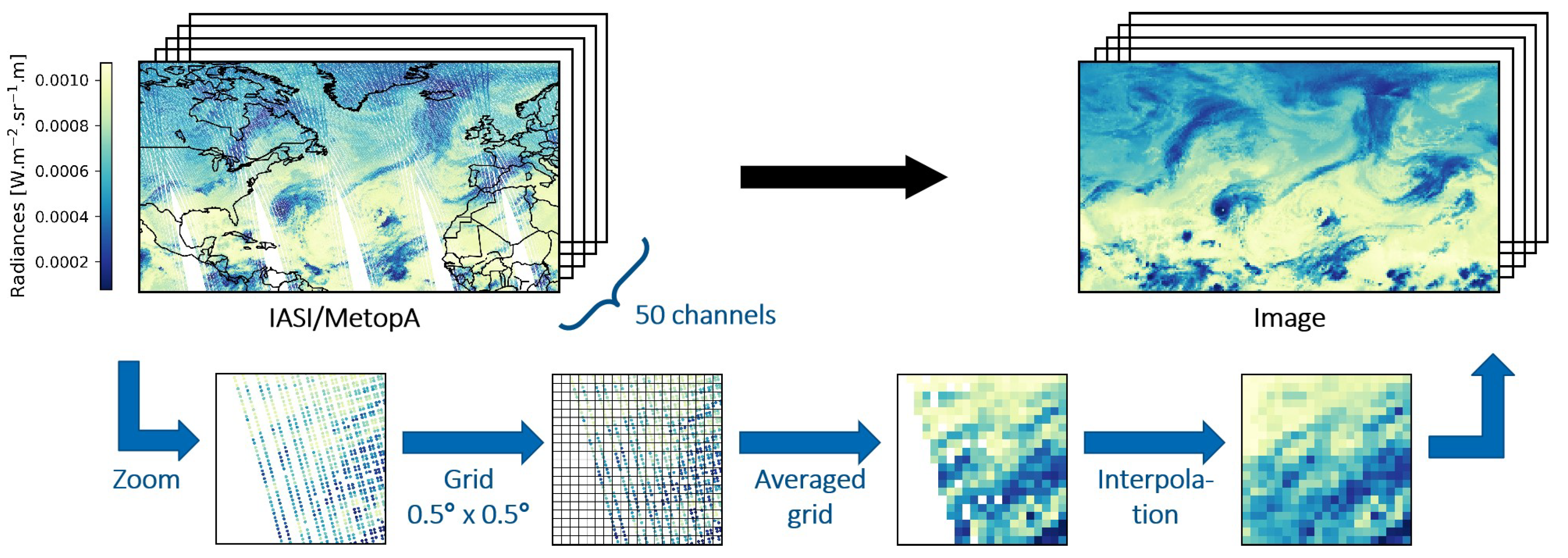
We attempt to detect TC activity in the North Atlantic Basin (between 5° and 75° N of latitude and between −110° and 18° E of longitude) using a deep learning object detection model applied to a TC dataset we created from IASI data. To our knowledge, no previous study attempted to exploit the added value of infrared sensors, such as IASI and their “raw” measurements, in the detection of TCs. The aim of the paper is to assess the performance of the YOLOv3 object detection model and the potential of the IASI data in the TC detection problem. The paper is organized as follows. In Section 2, we present the IASI data and the YOLOv3 model, as well as the dataset creation, from the processing of the IASI data to the labeling procedure. In Section 3, we describe the experiments performed on the model, assess its performance, and analyze its predictions. Finally, conclusions are presented in Section 4.

2. Materials and Methods

2.1. IASI Data

IASI is an instrument that flies onboard three Metop satellites, Metop A, B, and C, since 2006, 2012, and 2018, respectively (Metop-A was decommissioned in November 2021). One Metop satellite alone cannot fully cover the entire Earth daily, as shown in Figure 1a. Therefore for this study, to get full Earth coverage, gaps between two orbits were either interpolated (nearest-neighbor interpolation) or covered by the combination of two Metops, depending on the data availability. With about 14 orbits a day, the Metop satellites revolve around the Earth, each Metop being approximately half an orbit apart. Therefore, combining two Metop ensured a full Earth coverage as illustrated in Figure 1b. As Metop B data are only available since 9 March 2013, full coverage is only possible after this date. As to Metop C, data have been available since 21 September 2019. We used Metop A+B when Metop B was available but chose to use Metop B+C starting from the year 2020 as Metop A was decommissioned in late 2021. Choice of Metops is summarized in

Table 1. IASI/Metop used according to the period.

Period	IASI/Metop
2007/10/01–2013/03/08	A + interpolation
2013/03/09–2019/12/31	A + B
2020/01/01–2021/12/31	B + C

.

As the Metop satellites revolve around the Earth, each of the three IASI measures the infrared radiation emitted by the Earth and the atmosphere twice a day, with overpasses time at around 9:30 a.m. and 9:30 p.m. local time. The radiance spectral range extends from 15.5 to 3.62 µm, part of the thermal infrared, or 645 to 2760 cm${}^{-1}$ in wavenumber unit (inverse of the wavelength, used commonly in the research literature for IASI), sampled every 0.25 cm${}^{-1}$, providing a total of 8461 spectral channels or wavenumbers. In other words, each measurement, corresponding to a specific latitude/longitude coordinates (Figure 1c), is a spectrum composed of 8461 radiances, or brightness temperatures via Planck’s equation (assuming Earth is a black body), as illustrated in Figure 1d.

Among the 8641 wavenumbers, 49 have been selected to reduce the quantity of data, as the processing of a large quantity of data is computationally expensive. We chose to use wavenumbers/channels containing information related to temperature and clouds. The choice of the channels was made such as the information related to the retrieved quantity is maximal. For example, the wavenumbers chosen for clouds are those the most contaminated/sensitive typically to cloud presence. Those temperatures are chosen in regions of the spectrum where little other species absorb, allowing us to access the surface temperature of land when the sky is clear and the surface of the cloud in case of a cyclone, for example. Safieddine et al. [20] presented a selection of 100 wavenumbers sensitive to temperature ranked by sensitivity using an approach based on entropy reduction. We selected the 25 most sensitive. Whitburn et al. [21] provided a list of 45 wavenumbers sensitive to clouds. We chose the 24 wavenumbers whose position is distant from the 25 selected wavenumbers sensitive to temperature (Figure 2). The selected wavenumbers are listed in Appendix A. In short, we selected 25 “temperature” and 24 “cloud” sensitive channels containing good information content on each and low contamination from other molecules [20,21]. These are raw radiances, also called Level 1C data in TIR instrument jargon. To these 49 selected wavenumbers, we add one IASI product, the total water vapor column, for a total of 50 channels. The total water vapor column is not a raw measurement but a EUMETSAT product obtained by applying an algorithm to Level 1C data, called Level 2. Other attributes were considered, such as temperature at 200 hPa (about 12 km) or cloud top pressure, but could not be used due to many missing data.

2.2. YOLOv3 Model and Validation

Deep learning object detection models have attracted much research attention in recent years [22] and can be divided into two categories: single-stage detection models and two-stage models. Typical single-stage detectors are the YOLO (“You Only Look Once”) series [23,24,25] and SSD [26] while Region-based Convolutional Neural Network (R-CNN) [27], Fast R-CNN [28], and Faster R-CNN [29] are typical two-stage models. Usually, in two-stage detectors, one model is used to generate regions of interest in the input images, and a second model is used to classify and further refine the localization of the object, while single-stage detectors attempt to both locate and classify objects in images with a single network. Two-stage detectors generally have higher localization and object recognition accuracy, whereas single-stage detectors achieve higher inference speeds.

We used the YOLOv3 model [25], which is the third version of the YOLO series, where each version was improved. It has been proven successful with different kinds of datasets. Shakya et al. [30] suggested that YOLO could be used for the detection of cyclone location, and Pang et al. [31] successfully trained a YOLOv3 model to detect TC on meteorological satellite images with Average Precision (AP) of 81.39%. YOLOv3 uses Darknet-53 [25] as a backbone to extract image features: it is a convolutional neural network with 53 convolutional layers and residual connections. For the detection task, 53 more layers are stacked onto it, giving us a 106-layer fully convolutional underlying architecture for YOLOv3, with about 61.9 million parameters to set. YOLOv3 divides the input image into N × N grid cells. Each grid cell can predict B boxes, where B is the number of anchor boxes, which are pre-defined boxes. Instead of predicting boxes coordinates directly, the model predicts offsets from these anchor boxes. This simplifies the problem and makes it easier for the network to learn. These anchor boxes are the average characteristics of the groups of boxes found by K-means clustering performed on the training dataset. YOLOv3 uses 9 anchor boxes. For each box, several values are predicted:

• four offsets coordinates $t_x$, $t_y$, $t_w$, $t_h$ (center coordinates x,y of the box, width w, and height h)
• a confidence score reflecting how likely the box contains an object and how accurate is the box
• C values correspond to the class probabilities. In our case, C = 1, as we only have one class (TC).

For the detection part, YOLOv3 makes predictions at three different scales (as illustrated in Figure 3), which are precisely given by downsampling the dimensions of the input image by factors of 32, 16, and 8, respectively. This allows the model to detect objects of various sizes (small, medium, large) and helps address the issue of detecting small objects. As TCs vary in size, YOLOv3 multiple scales ensure accurate detection of both large-size and small-size TCs.

The object detector predicts multiple boxes, most of which are irrelevant or redundant, i.e., overlapping boxes predicting the same object. Ideally, for each object in the image, we must have a single box. To remove overlapping predictions, the Non-Maximum Suppression (NMS) [32] method is applied, which is a post-processing technique that selects the predictions with the maximum confidence score and suppresses all the other predictions having intersection over union (IoU) with the selected predictions greater than a threshold. The IoU is a number between 0 and 1 representing the amount of overlap between two boxes (see definition in Appendix B).

The loss function is used to compute the error between the predicted output and the ground truth and is essential for the training of the object detector. The loss is calculated for each of the three scales, then summed up for backpropagation to train the model. The loss is the combination of three loss functions: the mean squared error loss comparing the predicted box coordinates and the expected box coordinates (ground truth), the binary cross-entropy loss for the box confidence score, and the binary cross-entropy loss for the box classification. However, the loss for the classification will always be null in our case since we only have one class (TC).

To evaluate the performance of the model, we used the Average Precision (AP), which is a metric commonly used in the object detection domain. This metric is based on the IoU. If the IoU between a predicted box and a ground truth is greater than a threshold T${}_{\mathrm{IoU}}$, the detection is considered as a True Positive (TP), else as a False Positive (FP). It can be noticed that predictions whose confidence score is lesser than a threshold T${}_{\mathrm{conf}}$ are discarded to ensure a minimum confidence score for the predictions. False Negatives (FN) are the ground truths that have not been detected by the model. Using these concepts, which are summarized in Appendix B, we can define precision (Equation (A1)) and recall (Equation (A2)). We can then define the Average Precision (AP), which is the area under the Precision–Recall curve. To obtain this curve, the predictions are sorted according to their confidence score (descending order), then the precision and recall of the accumulated predictions are calculated [33]. Therefore AP is a metric to evaluate precision and recall in different T${}_{\mathrm{conf}}$ values. A perfect detector has an AP equal to 1, i.e., the detector finds all the TCs without making false detection of TC. An object detection model is considered good if its precision stays high as recall increases. A poor object detector needs to increase the number of predictions to retrieve all ground truth objects. As a result, the number of FP increases which leads to lower precision. That’s why the Precision–Recall curve usually starts with high precision values, decreasing as recall increases. As AP depends on the IoU threshold T${}_{\mathrm{IoU}}$ to determine whether a prediction is correctly predicted, we can define AP@.5 (resp. AP@.1), which is the AP with T${}_{\mathrm{IoU}}$ = 0.5 (resp. T${}_{\mathrm{IoU}}$ = 0.1), meaning that a prediction must have IoU greater or equal than 0.5 (resp. 0.1) to be considered as a True Positive.

2.3. Image Processing and Labeling

To prepare the data for the object detection model, we show in Figure 4 an example of one channel of IASI (in radiance or “raw” units) for half a day. Our area of focus is the North Atlantic Basin, a region known for high cyclonic activity, and the radiances value (the colors) reflects the presence of clouds: lower radiances are recorded in areas with high cloud cover and low temperatures, reflecting as such a possible presence of a cyclone. In fact, for each channel (shown in Figure 2), we can construct a similar map. This is also illustrated in Figure 4.

However, the raw data can not be used as it is to train the object detection model, as the latter expects images as input. Therefore we constructed “images” from the IASI data. In computer science, a typical RGB image consists of a stack of three matrices called channels, each one defining one of the red-green-blue color components. The combination of the three channels gives the color of each pixel. In this study, the concept of image is used identically: an IASI image is a stack of matrices, with each matrix defining one of the selected IASI channels (Figure 2). As the combination of IASI channels does not have any graphical meaning, each channel is individually represented, as shown in Figure 4.

To construct the IASI images, the raw data were averaged in a 0.5° × 0.5° grid, then interpolated if necessary (nearest-neighbor interpolation) to fill the empty cells as illustrated in Figure 4. This process was applied to each channel, which resulted in matrices of shape 140 × 256 × 50. We performed tests with 1° × 1° as well as 0.25° × 0.25° grids (not shown here). 0.5° × 0.5° was the best compromise to get a small cell size and avoid a large number of cells with no value.

To train the object detection model, images need to be labeled. A bounding box (bbox) surrounding each TC must be defined. HURDAT2 (HURricane DATabase 2nd generation) [34] from the National Oceanic and Atmospheric Administration (NOAA) was used to locate TC positions in the images (available at www.nhc.noaa.gov/data/hurdat, accessed on 23 May 2022). It gathers re-analyzed tracks of tropical and subtropical cyclones in the Atlantic Basin since 1851 at 6-hour intervals. More precisely, the HURDAT2 database gives:

• cyclone center location (latitude/longitude) at 0, 6, 12, and 18 h UTC
• 34 knots (about 63 km/h) wind radii maximum extent in northeastern, southeastern, southwestern, and northwestern quadrant (in nautical miles), i.e., for each of the directions, the distance until which the wind speed is more than 34 knots is given.

Bounding boxes center were directly given by the HURDAT2 database. We deduced the size of the bounding boxes based on the wind radii values as shown in Figure 5. As each wind radius gives the distance (from the cyclone center) until which the wind speed is less than 34 knots, we simply keep the maximum distance in the four directions north, south, east, and west. We then convert the distance from nautical miles to degrees of longitude (north/south direction) or latitude (east/west direction), then add/subtract it to the center coordinate to obtain the limits of the bounding box. These bboxes constitute image labels. Because this method requires the 34 knots wind radii maximum extent to label the images, only TCs with maximum sustained wind of at least 34 knots were taken into account in this study. With IASI data available starting October 2007 and the HURDAT2 database ending in 2021 (since the access date), we considered the period 2007/10/01–2021/12/31 for our study. During this period, a total of 234 TCs were tracked and listed in the database for a total of 4935 TCs positions (cyclone lifespan generally last several days).

Matching IASI and HURDAT2 data was not straightforward. As HURDAT2 provides TCs position at 6 h-interval (0, 6, 12, and 18 h UTC) while IASI passes over each location 2 times a day at 9:30 a.m. and 9:30 p.m. local time (with data provided in UTC), there can be a discrepancy between given TC position and observed IASI data, resulting in cyclone center that might not be precisely over the correct location or having two TC positions being matched to the same IASI overpass. For instance, the position for a TC at 6 h and 12 h UTC could be matched to the same IASI overpass at 9:30 a.m. local time. In that case, we merged the two boxes from 6 h and 12 h UTC, resulting in a larger final box (as illustrated in Figure A2). If two positions are matched to the same IASI overpass, then one of them necessarily happened before the selected IASI overpass, while the other happened after. This is explained and illustrated in Appendix C. As a result, the TC is ensured to be inside the merged box and might also encompass more than necessary. However, as said in [35], this is preferable to encompassing too little of the TC to prevent the model from missing any key features. The dataset creation procedure is summarized in Appendix D.

Based on IASI data and matched hurricane data from HURDAT2, we found over the period 2007–2021 (Table 1), 1985 images of shape 140 × 256 × 50 and 2594 labels/boxes in total (several TCs can be in the same image). The dataset was divided into train (70%), validation (15%), and test (15%) sets. The distribution of each split (train, validation, or test) was carefully chosen to avoid unwanted bias. Indeed, since the dataset is based on tracks of TCs, two successive images can be quite similar if the TC does not move much. If we divide the dataset randomly, these similar images might be distributed in train and test, which could bias the results, as there will be images in test that are too similar to images in train. The dataset was, therefore, sampled randomly by years while ensuring the correct ratio for each set (see

Table 2. Years distribution in the train, validation, and test set. The dataset is composed of 1985 images for the period 2007–2021.

Set	Years
Train (70% of the data)	2007, 2008, 2009, 2010, 2011, 2012, 2013, 2014, 2016, 2017, 2021
Validation (15% of the data)	2015, 2020
Test (15% of the data)	2018, 2019

for years distribution in each set). Both training and validation sets were used to build the model, i.e., to select the best hyperparameters. Hyperparameters are variables that determine the network architecture and how the network is trained, such as the number of training iterations, for instance. The test set was kept hidden from the entire training and validation process to ensure an unbiased evaluation of the model.

3. Results and Discussion

3.1. Description of Experiments

In this work, two experiments were conducted:

• Experiment A: First experiment consisted in using only three carefully selected channels from the 50 previously selected (Figure 2) to keep the original architecture of the YOLOv3 model unchanged, the latter expecting input images of three channels.
• Experiment B: Second experiment considered all 50 selected channels and reduced them to three using a specific NN architecture: an autoencoder.

These experiments were run on an Nvidia Tesla V100 16 GB GPU from the Jean Zay supercomputer installed at the Institute for Development and Resources in Intensive Scientific Computing (IDRIS). The code used for the YOLOv3 model is an implementation from Ultralytics [36] that we adapted to fit our dataset format. As YOLOv3 expects square input matrices and since our images are rectangular (140 × 256), the images were padded with zeros to ensure a square input of 256 × 256. Input images were also transformed by applying Z-score normalization (or standardization) to have each channel on the same scale. The mean and standard deviation were calculated from the training set only to keep the validation and test sets as unseen data, then each sample of the entire dataset was transformed by subtracting the mean and dividing by the standard deviation. This is a standard procedure to compare the images better and reduce the number of significant figures within the radiance values, shown in Figure 2. After normalization, images corresponded to values between −3 and 6 approximately, with most values between −2.5 and 2. In the following figures, we show the normalized images. Therefore, their values do not correspond to the radiances and have no particular meaning, and as such, no unit is assigned to them. This makes no difference visually and only changes the range of values.

3.2. Experiment A: Three Channels

For experiment A, we selected the most sensitive “temperature” channel (wavenumber at 969.75 cm${}^{-1}$) according to the sensitivity ranking from Safieddine et al. [20], one “cloud” channel (wavenumber at 1006.5 cm${}^{-1}$) randomly chosen as there was no ranking available, and lastly the water vapor column, for a total of three channels.

First training achieved Average Precision at threshold 0.1 (AP@.1) of 55.67% and AP@.5 of 15.25% and resulted in overfitting, i.e., the YOLOv3 modeled the training data too well, to the extent that it could not perform accurately against unseen data. It memorized the training data without learning the underlying pattern, which defeats its purpose. One of the potential causes of overfitting is the lack of training data. Indeed, deep learning models with a large number of parameters usually require a large quantity of data to have good performance. Our dataset contains about 1300 images, which might not be sufficient for the YOLOv3, composed of about 61.9 million parameters to learn.

To improve performance, we used transfer learning and data augmentation. Transfer learning is a method where we reuse a pretrained model as the starting point for a model on a new related task. Instead of learning the model from scratch, we initialize it using the pretrained model. In our case, we used a pretrained YOLOv3 trained on the Common Object in Context (COCO) [37] dataset, which is a large-scale object detection, segmentation, key-point detection, and captioning dataset containing images of everyday objects (e.g., persons, cars, etc.). The COCO dataset is often used to benchmark models and compare their performance. Using pretrained weights on a large dataset could mitigate the problem of insufficient training data and help prevent overfitting by transferring the knowledge from the source to the target model. For its part, data augmentation is a process of artificially increasing the amount of data by generating new data points from existing data. In computer vision, this is typically done by altering existing images, for instance by rotating or cropping input images or adding noise [38]. We tried several types of augmentation and the one that gave the best results was flipping horizontally and/or vertically images randomly chosen.

Table 3. AP scores on the test set for both experiment A (Section 3.2) and experiment B (Section 3.3).

Experiment	Pretrained Weights	Flip	AP@.1 (%)	AP@.5 (%)
	No	No	55.67	15.25
A	Yes	No	73.58	29.36
	Yes	Yes	76.00	33.84
B	Yes	Yes	78.31	31.05

shows quantitatively how these two methods helped improve model performance, with AP increasing at each addition. Finally, the model achieved AP@.1 of 76% and AP@.5 of 33.84%. Figure 6 shows some predictions with their confidence score in red as well as the ground truth in black. We can observe some really close predictions in panels a and b, with the predictions being really close to the ground truth. A prediction that does not detect any ground truth (False Positive) was made on the top-right of panel c. However, its confidence score is relatively low (0.13) compared, for instance, to the other prediction on the same panel (0.78), hinting at the model not being confident over this prediction, which is justified as there is no ground truth there.

However, it can be noticed that the model struggles to achieve accurate predictions, as using a stricter IoU threshold (0.5) for the AP resulted in poorer performance compared to AP at threshold 0.1, showing the model detects TCs but is imprecise. The higher the threshold is, the more precise the predicted box must be to count as a TP, as Figure 6d shows. Although the predicted box (in red) is roughly centered around the event, its size is much smaller than the ground truth (in black): this is sufficient to count as a correct prediction with an IoU threshold of 0.1, but not for the severer threshold of 0.5. Figure 6c shows another example of prediction (in the middle of the panel); this time, the size of the prediction is larger than the ground truth. The prediction encompasses the ground truth, but its size is too large, resulting in the prediction being identified as TP for AP@.1 but as FP for AP@.5.

To determine whether the model tends to be more successful with a particular box size, we analyzed the distribution of the ground truth surface area, as shown in Figure 7a. The panel shows the distribution in the test set of the ground truth surface area (in blue), as well as the distribution of the ground truth that has been correctly predicted by the YOLOv3 with IoU threshold of 0.1 (in orange) or 0.5 (in green). The discrepancy between the distribution with the IoU threshold of 0.1 and 0.5 mostly lies in the ground truth of small size (<100 px) and large size (≥800 px), meaning the model struggles to make accurate predictions with these box sizes. It is indeed more challenging to detect small boxes as even a slight shift in the prediction can change whether the prediction will be accounted as TP or FP. On the other hand, the issue with missing large-size ground truth might be due to the fact that the model has not seen a lot of large TCs during training, as shown in Figure 7b: the distribution of the ground truth surface area in train set shows that the frequency of large boxes is indeed low, the dataset being mostly composed of the ground truth of smaller size.

3.3. Experiment B: Compressing 50 Channels

To exploit all the 50 selected channels, we used an autoencoder, a type of NN used to reduce the dimensionality of the input data by compressing the information into a smaller space called latent space. It is composed of two distinct parts: an encoder and a decoder. The encoder is used to compress the input data into the latent space while the decoder reconstructs the input data from the latent space. Generally, autoencoders reduce the height and width of the input image, but in this work, we focused on reducing the number of input channels so that the latent space is compatible with YOLOv3 (input size [140, 256, 3]). At first, we used all 50 channels as input to the autoencoder to obtain a latent space of 3 channels. However, we obtained better results when removing the water vapor from the autoencoder input data. Therefore we used the autoencoder to compress the 49 “temperature” and “cloud” channels into 2 channels to obtain latent space of size [140, 256, 2], to which we add the water vapor column, providing the same input shape as expected by the YOLOv3. The autoencoder architecture used in this paper is described in Appendix E. Training such NN requires a loss function to quantify the difference between the input and the reconstruction. The autoencoder was trained with Mean Squared Error (MSE) loss for 200 epochs. At the end of the training, we obtained an MSE of 0.004. Figure 8 gives an example of side by side comparison between an original image from the validation set (panel a) and its reconstruction by the autoencoder (panel b) for one channel. Visually, images are almost identical, suggesting the model does a good job of reproducing the input image. This is confirmed by panel c, which shows the relative difference between the original and the reconstruction. The mean relative difference over the whole image is 5.2%, suggesting the good performance of the autoencoder.

Figure 9 compares all the normalized original images I${}_O$ from the validation set with their reconstruction by the autoencoder I${}_R$. A good agreement was achieved, with a standard deviation of the difference I${}_O$− I${}_R$ equal to 0.065 and a correlation coefficient close to 1 (0.998). This shows that regardless of the channel, the autoencoder could successfully reconstruct the original images from the latent space, which means the information contained in the 49 input channels has been successfully encoded and compressed into 2 channels. Figure 10 shows the latent space for one image (panels b and c). It can be observed that the patterns of the original image (panel a) are recognizable in the latent space, such as the curve in the middle of the figure or the form in the middle top. With the latent space and the water vapor column (shown in panel d), we obtained the new input data for the YOLOv3.

Results are shown in Table 3 (last line). YOLOv3 achieved AP@.1 of 78.31% and AP@.5 of 31.05%. As in experiment A, the model still struggles to achieve accurate predictions, as AP achieved poorer performance with an IoU threshold of 0.5 than with a threshold of 0.1. Results could be further optimized by fine-tuning the hyperparameters.

The advantage of experiment B is higher AP@.1 compared to experiment A, as we can observe an increase of 2.31 percentage points (pp). However, experiment B requires training the autoencoder first, adding more steps and complexity to the method, while experiment A is more straightforward. It can be noticed that experiment B led to lower AP@.5 than experiment A (−2.79 pp). Therefore, even though AP@.1 increased in experiment B, the model seems to struggle even more in making accurate predictions. However, with the large discrepancy between AP@.1 and AP@.5 in both experiments, with AP@.5 being relatively low compared to AP@.1 (more than 40 pp of difference), the model seems more predisposed to be used to detect TCs, even if predictions lack in precision (predictions too large or too small, or predictions slightly off). We would, therefore, favor the method used in experiment B even if AP@.5 is higher in experiment A.

Gardoll et al. [39] summarized eight years of applying DL models for the classification, detection, or segmentation of hurricanes from satellite or model data. Among these studies, the one by Pang et al. [31] aims at object detection: the authors used the YOLOv3, combined with a deep convolutional generative adversarial network (DCGAN) for data augmentation, to detect TCs and obtained a mean AP@.5 (mean AP is the average of AP obtained for each class, in our case AP and mean AP are the same since we have only one class) of 81.39%. Shi et al. [13] used the Single Shot Detector (SSD) model and obtained a mean AP@.5 of 79.34–86.64%. Compared to these previous studies, we obtained lower metric values. However, these studies focused on different regions or used different parameters as input in the model, making a direct comparison of their performance very difficult. First, Pang et al. trained their model with satellite images, but the region of interest is quite different: we focused on a fixed region (North Atlantic Basin), while Pang et al. used zoomed images centered on TCs of the Southwest Pacific area. Shi et al. used ERA5 data with variables such as mean sea level pressure or vorticity that characterize cyclones and are not present in our training dataset, as we focused on using mostly raw radiances from IASI.

4. Conclusions

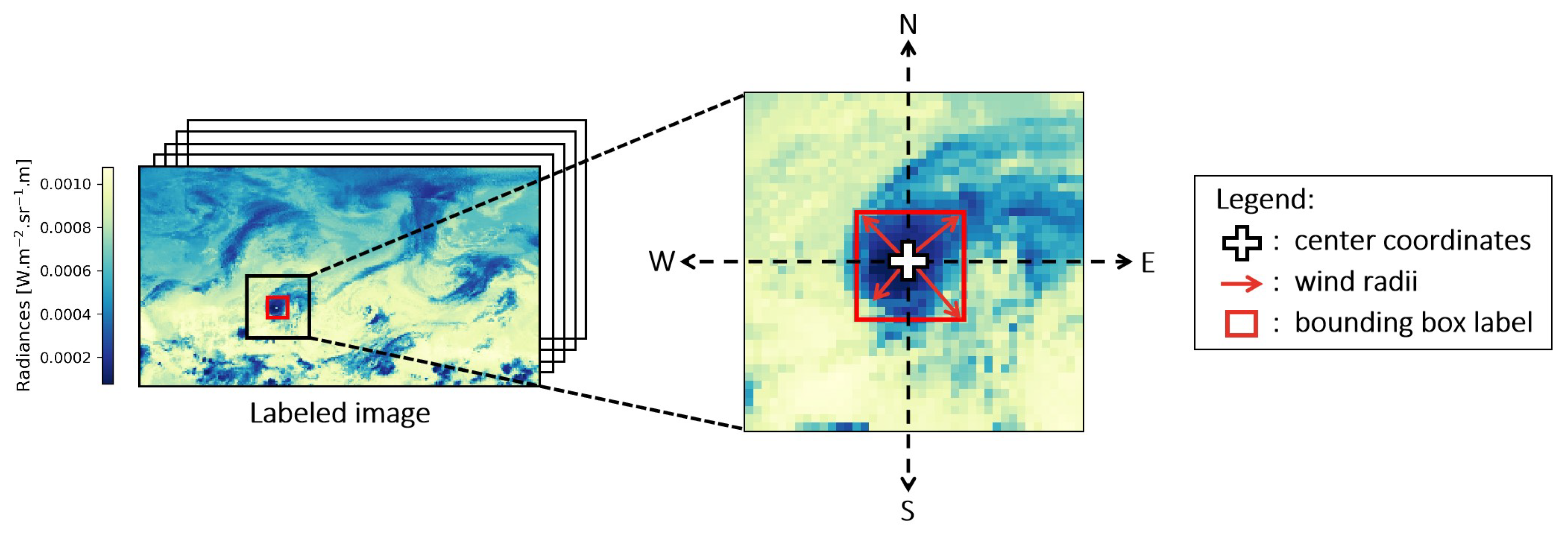
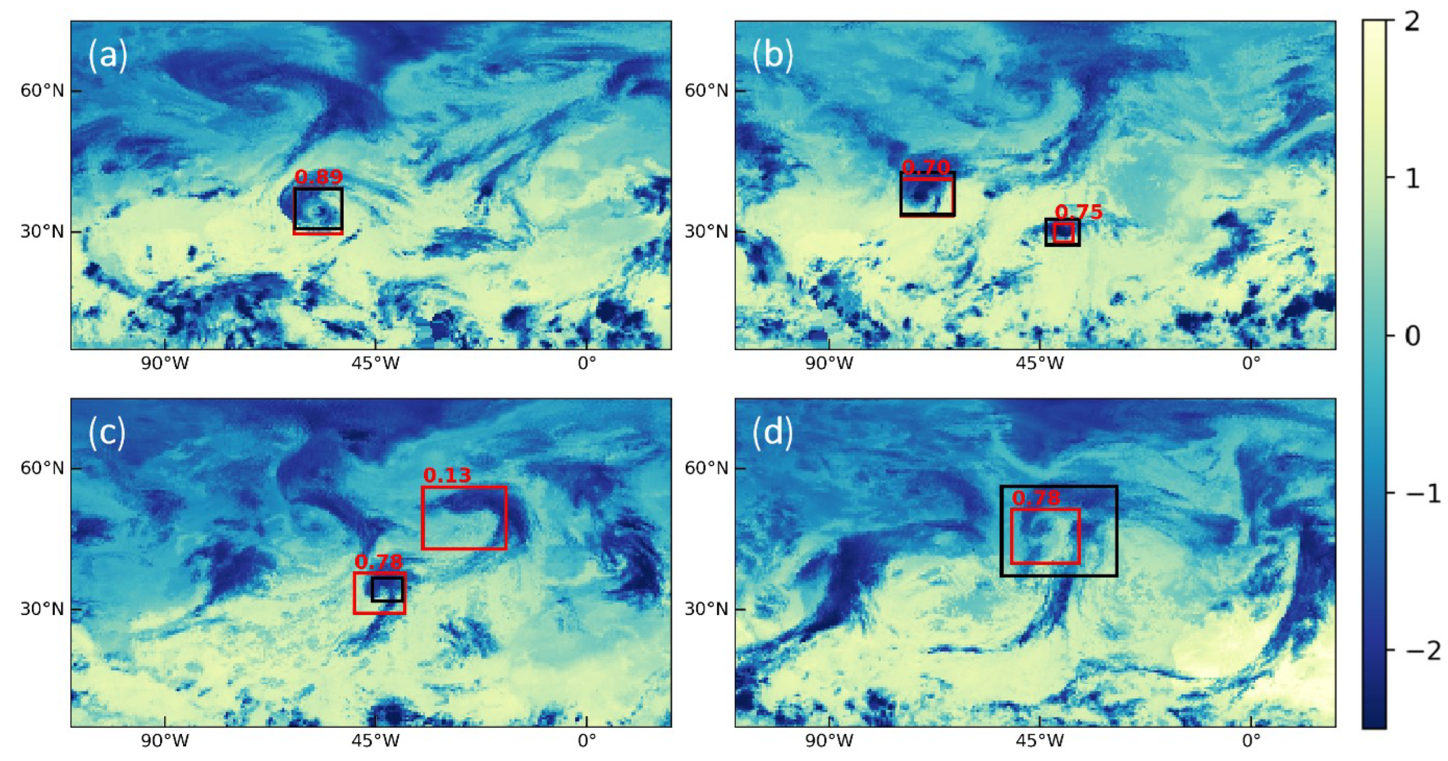
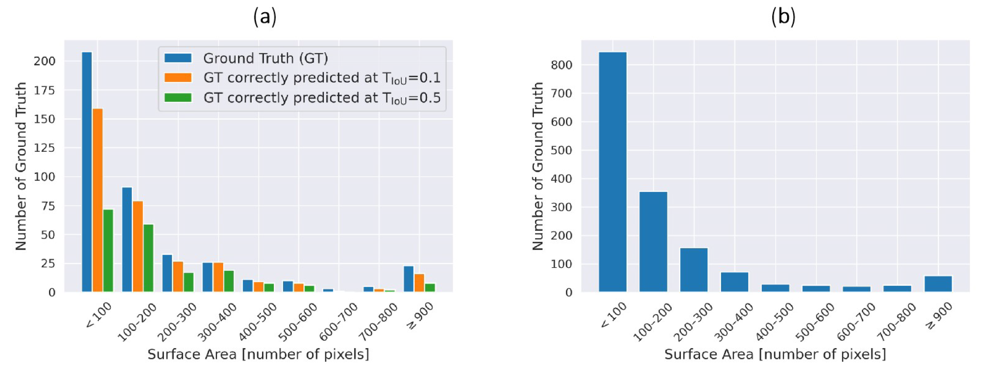
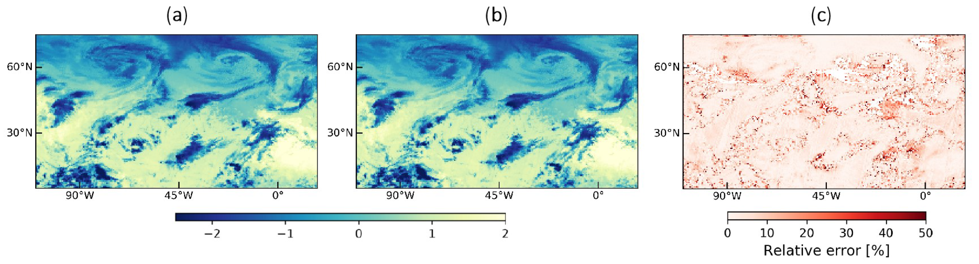
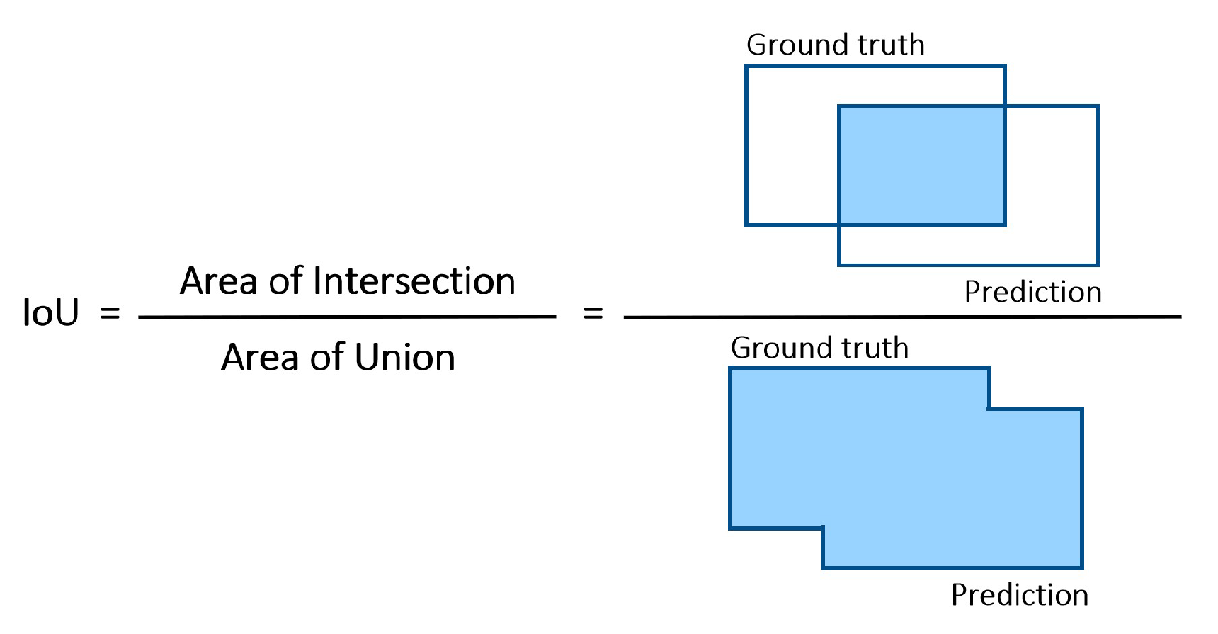
In this paper, we attempted to detect TCs in the North Atlantic Basin. We proposed a framework to process a selection of 50 channels from IASI radiance data into multi-channel images, as well as a labeling procedure using the HURDAT2 database. YOLOv3 object detection model has been trained on this dataset, firstly using three channels, then using an autoencoder to exploit all 50 channels. IASI data are not combined with other instruments’ data to form the dataset, and no wind data are used. We achieved promising results with Average Precision at threshold 0.1 (AP@.1) of 78.31%, although AP@.5 gave lower results (31.05%), hinting at a lack of precision of the model in its predictions, more particularly in the size of the predicted boxes.

The model could further be optimized by fine-tuning the hyperparameters. Application of the proposed framework could be extended to other models, such as the two-stage model Faster R-CNN [29] or other single-stage models such as SSD [26]. Further improvements to the input data could be explored, such as using other IASI products or channels, trying different interpolation methods (linear, cubic), or applying more advanced data augmentation techniques. For instance, Pang et al. [31] used a deep convolutional generative adversarial network (DCGAN) to generate new images. Our method could be adapted to other regions outside the North Atlantic Basin, provided that tracks of TCs are available there. Other similar sensors to IASI could be used instead, such as the Atmospheric InfraRed Sounder (AIRS), the Moderate Resolution Imaging Spectroradiometer (MODIS), the Spinning Enhanced Visible and Infrared Imager (SEVIRI), on polar orbits (two crossing per day) or on geostationary orbits (many observations per day).

This study shows the ability of TIR instruments to act as valuable inputs into detection models. The IASI mission is planned to fly till at least 2028. It will be completed by the IASI-New Generation series of instruments [40,41] that will be launched on the Metop-Second Generation series of satellites starting 2024–2025 and running until at least 2045. A new era of TC detection will, therefore, be possible from infrared sensors for decades to come.

References

1. Atlantic Oceanographic and Meteorological Laboratory. What Is a Tropical Cyclone, Tropical Disturbance, Tropical Depression, Tropical Storm, Hurricane, and Typhoon? 2021. Available online: https://www.aoml.noaa.gov/hrd-faq/#what-is-a-hurricane (accessed on 13 November 2022).
2. Vitart, F.; Anderson, J.L.; Stern, W.F. Simulation of Interannual Variability of Tropical Storm Frequency in an Ensemble of GCM Integrations. J. Clim. 1997, 10, 745–760. [Google Scholar] [CrossRef]
3. Bosler, P.A.; Roesler, E.L.; Taylor, M.A.; Mundt, M.R. Stride Search: A general algorithm for storm detection in high-resolution climate data. Geosci. Model Dev. 2016, 9, 1383–1398. [Google Scholar] [CrossRef] [Green Version]
4. Ullrich, P.A.; Zarzycki, C.M. TempestExtremes: A framework for scale-insensitive pointwise feature tracking on unstructured grids. Geosci. Model Dev. 2017, 10, 1069–1090. [Google Scholar] [CrossRef] [Green Version]
5. Bourdin, S.; Fromang, S.; Dulac, W.; Cattiaux, J.; Chauvin, F. Intercomparison of four tropical cyclones detection algorithms on ERA5. Geosci. Model Dev. 2022, 15, 6759–6786. [Google Scholar] [CrossRef]
6. Li, J.; Bao, Q.; Liu, Y.; Wu, G.; Lei, W.; He, B.; Wang, X.; Li, J. Evaluation of FAMIL2 in Simulating the Climatology and Seasonal-to-Interannual Variability of Tropical Cyclone Characteristics. J. Adv. Model. Earth Syst. 2019, 11, 1117–1136. [Google Scholar] [CrossRef]
7. Zhao, M.; Held, I.; Lin, S.J.; Vecchi, G. Simulations of Global Hurricane Climatology, Interannual Variability, and Response to Global Warming Using a 50-km Resolution GCM. J. Clim.-J. Clim. 2009, 22, 6653–6678. [Google Scholar] [CrossRef] [Green Version]
8. Li, J.; Bao, Q.; Liu, Y.; Wang, L.; Yang, J.; Wu, G.; Wu, X.; He, B.; Wang, X.; Zhang, X.; et al. Effect of horizontal resolution on the simulation of tropical cyclones in the Chinese Academy of Sciences FGOALS-f3 climate system model. Geosci. Model Dev. 2021, 14, 6113–6133. [Google Scholar] [CrossRef]
9. Kumler-Bonfanti, C.; Stewart, J.; Hall, D.; Govett, M. Tropical and Extratropical Cyclone Detection Using Deep Learning. J. Appl. Meteorol. Climatol. 2020, 59, 1971–1985. [Google Scholar] [CrossRef]
10. Neumann, C.J. An Alternate to the HURRAN (Hurricane Analog) Tropical Cyclone Forecast System. 1972. Available online: https://repository.library.noaa.gov/view/noaa/3605 (accessed on 13 November 2022).
11. Knaff, J.A.; Sampson, C.R.; Musgrave, K.D. Statistical Tropical Cyclone Wind Radii Prediction Using Climatology and Persistence: Updates for the Western North Pacific. Weather. Forecast. 2018, 33, 1093–1098. [Google Scholar] [CrossRef]
12. Bessafi, M.; Lasserre-Bigorry, A.; Neumann, C.J.; Pignolet-Tardan, F.; Payet, D.; Lee-Ching-Ken, M. Statistical Prediction of Tropical Cyclone Motion: An Analog–CLIPER Approach. Weather Forecast. 2002, 17, 821–831. [Google Scholar] [CrossRef]
13. Shi, M.; He, P.; Shi, Y. Detecting Extratropical Cyclones of the Northern Hemisphere with Single Shot Detector. Remote Sens. 2022, 14, 254. [Google Scholar] [CrossRef]
14. Clerbaux, C.; Boynard, A.; Clarisse, L.; George, M.; Hadji-Lazaro, J.; Herbin, H.; Hurtmans, D.; Pommier, M.; Razavi, A.; Turquety, S.; et al. Monitoring of atmospheric composition using the thermal infrared IASI/MetOp sounder. Atmos. Chem. Phys. 2009, 9, 6041–6054. [Google Scholar] [CrossRef] [Green Version]
15. Hilton, F.; Armante, R.; August, T.; Barnet, C.; Bouchard, A.; Camy-Peyret, C.; Capelle, V.; Clarisse, L.; Clerbaux, C.; Coheur, P.F.; et al. Hyperspectral Earth Observation from IASI: Five Years of Accomplishments. Bull. Am. Meteorol. Soc. 2012, 93, 347–370. [Google Scholar] [CrossRef]
16. Clarisse, L.; R’honi, Y.; Coheur, P.F.; Hurtmans, D.; Clerbaux, C. Thermal infrared nadir observations of 24 atmospheric gases. Geophys. Res. Lett. 2011, 38, L10802. [Google Scholar] [CrossRef] [Green Version]
17. Goldberg, M.; Ohring, G.; Butler, J.; Cao, C.; Datla, R.; Doelling, D.; Gärtner, V.; Hewison, T.; Iacovazzi, B.; Kim, D.; et al. The Global Space-Based Inter-Calibration System. Bull. Am. Meteorol. Soc. 2011, 92, 467–475. [Google Scholar] [CrossRef]
18. Bouillon, M.; Safieddine, S.; Hadji-Lazaro, J.; Whitburn, S.; Clarisse, L.; Doutriaux-Boucher, M.; Coppens, D.; August, T.; Jacquette, E.; Clerbaux, C. Ten-Year Assessment of IASI Radiance and Temperature. Remote Sens. 2020, 12, 2393. [Google Scholar] [CrossRef]
19. George, M.; Clerbaux, C.; Hurtmans, D.; Turquety, S.; Coheur, P.F.; Pommier, M.; Hadji-Lazaro, J.; Edwards, D.P.; Worden, H.; Luo, M.; et al. Carbon monoxide distributions from the IASI/METOP mission: Evaluation with other space-borne remote sensors. Atmos. Chem. Phys. 2009, 9, 8317–8330. [Google Scholar] [CrossRef] [Green Version]
20. Safieddine, S.; Parracho, A.C.; George, M.; Aires, F.; Pellet, V.; Clarisse, L.; Whitburn, S.; Lezeaux, O.; Thépaut, J.N.; Hersbach, H.; et al. Artificial Neural Networks to Retrieve Land and Sea Skin Temperature from IASI. Remote Sens. 2020, 12, 2777. [Google Scholar] [CrossRef]
21. Whitburn, S.; Clarisse, L.; Crapeau, M.; August, T.; Hultberg, T.; Coheur, P.F.; Clerbaux, C. A CO2-free cloud mask from IASI radiances for climate applications. Atmos. Meas. Tech. Discuss. 2022, 2022, 1–22. [Google Scholar] [CrossRef]
22. Zhao, Z.Q.; Zheng, P.; Xu, S.t.; Wu, X. Object Detection with Deep Learning: A Review. IEEE Trans. Neural Netw. Learn. Syst. 2019, 30, 3212–3232. [Google Scholar] [CrossRef]
23. Redmon, J.; Divvala, S.; Girshick, R.; Farhadi, A. You Only Look Once: Unified, Real-Time Object Detection. In Proceedings of the 2016 IEEE Conference on Computer Vision and Pattern Recognition (CVPR), Las Vegas, NV, USA, 27–30 June 2016; pp. 779–788. [Google Scholar] [CrossRef] [Green Version]
24. Redmon, J.; Farhadi, A. YOLO9000: Better, Faster, Stronger. In Proceedings of the 2017 IEEE Conference on Computer Vision and Pattern Recognition (CVPR), Honolulu, HI, USA, 21–26 July 2017; pp. 6517–6525. [Google Scholar] [CrossRef] [Green Version]
25. Redmon, J.; Farhadi, A. YOLOv3: An Incremental Improvement. arXiv 2018, arXiv:1804.02767. [Google Scholar] [CrossRef]
26. Liu, W.; Anguelov, D.; Erhan, D.; Szegedy, C.; Reed, S.; Fu, C.Y.; Berg, A.C. SSD: Single Shot MultiBox Detector. In Computer Vision – ECCV 2016; Springer International Publishing: Cham, Switzerland, 2016; pp. 21–37. [Google Scholar] [CrossRef] [Green Version]
27. Girshick, R.; Donahue, J.; Darrell, T.; Malik, J. Rich Feature Hierarchies for Accurate Object Detection and Semantic Segmentation. In Proceedings of the 2014 IEEE Conference on Computer Vision and Pattern Recognition (CVPR), Columbus, OH, USA, 23–28 June 2014; pp. 580–587. [Google Scholar] [CrossRef] [Green Version]
28. Girshick, R. Fast R-CNN. In Proceedings of the 2015 IEEE International Conference on Computer Vision (ICCV), Santiago, Chile, 7–13 December 2015; pp. 1440–1448. [Google Scholar] [CrossRef]
29. Ren, S.; He, K.; Girshick, R.; Sun, J. Faster R-CNN: Towards Real-Time Object Detection with Region Proposal Networks. IEEE Trans. Pattern Anal. Mach. Intell. 2017, 39, 1137–1149. [Google Scholar] [CrossRef] [Green Version]
30. Shakya, S.; Kumar, S.; Goswami, M. Deep Learning Algorithm for Satellite Imaging Based Cyclone Detection. IEEE J. Sel. Top. Appl. Earth Obs. Remote. Sens. 2020, 13, 827–839. [Google Scholar] [CrossRef]
31. Pang, S.; Xie, P.; Xu, D.; Meng, F.; Tao, X.; Li, B.; Li, Y.; Song, T. NDFTC: A New Detection Framework of Tropical Cyclones from Meteorological Satellite Images with Deep Transfer Learning. Remote Sens. 2021, 13, 1860. [Google Scholar] [CrossRef]
32. Neubeck, A.; Van Gool, L. Efficient Non-Maximum Suppression. In Proceedings of the 18th International Conference on Pattern Recognition (ICPR’06), Hong Kong, China, 20–24 August 2006; Volume 3, pp. 850–855. [Google Scholar] [CrossRef]
33. Padilla, R.; Passos, W.L.; Dias, T.L.B.; Netto, S.L.; da Silva, E.A.B. A Comparative Analysis of Object Detection Metrics with a Companion Open-Source Toolkit. Electronics 2021, 10, 279. [Google Scholar] [CrossRef]
34. Landsea, C.W.; Franklin, J.L. Atlantic hurricane database uncertainty and presentation of a new database format. Mon. Weather Rev. 2013, 141, 3576–3592. [Google Scholar] [CrossRef]
35. Bonfanti, C.; Trailovic, L.; Stewart, J.; Govett, M. Machine Learning: Defining Worldwide Cyclone Labels for Training. In Proceedings of the 2018 21st International Conference on Information Fusion (FUSION), Cambridge, UK, 10–13 July 2018; pp. 753–760. [Google Scholar] [CrossRef]
36. Jocher, G.; Kwon, Y.; guigarfr; perry0418; Veitch-Michaelis, J.; Ttayu; Suess, D.; Baltacı, F.; Bianconi, G.; IlyaOvodov; et al. ultralytics/yolov3: V9.5.0-YOLOv5 v5.0 Release Compatibility Update for YOLOv3. 2021. Available online: https://zenodo.org/record/4681234#.Y8YWHnZByUk (accessed on 14 June 2021).
37. Lin, T.Y.; Maire, M.; Belongie, S.; Bourdev, L.; Girshick, R.; Hays, J.; Perona, P.; Ramanan, D.; Zitnick, C.L.; Dollár, P. Microsoft COCO: Common Objects in Context. In Computer Vision—ECCV 2014; Springer: Cham, Switzerland, 2014. [Google Scholar] [CrossRef] [Green Version]
38. Shorten, C.; Khoshgoftaar, T.M. A survey on image data augmentation for deep learning. J. Big Data 2019, 6, 60. [Google Scholar] [CrossRef]
39. Gardoll, S.; Boucher, O. Classification of tropical cyclone containing images using a convolutional neural network: Performance and sensitivity to the learning dataset. Geosci. Model Dev. 2022, 15, 7051–7073. [Google Scholar] [CrossRef]
40. Clerbaux, C.; Crevoisier, C. New Directions: Infrared remote sensing of the troposphere from satellite: Less, but better. Atmos. Environ. 2013, 72, 24–26. [Google Scholar] [CrossRef]
41. Crevoisier, C.; Clerbaux, C.; Guidard, V.; Phulpin, T.; Armante, R.; Barret, B.; Camy-Peyret, C.; Chaboureau, J.P.; Coheur, P.F.; Crépeau, L.; et al. Towards IASI-New Generation (IASI-NG): Impact of improved spectral resolution and radiometric noise on the retrieval of thermodynamic, chemistry and climate variables. Atmos. Meas. Tech. 2014, 7, 4367–4385. [Google Scholar] [CrossRef]
Figure 1. (a) IASI observation points for Metop A in the North Atlantic Basin ([5° 75° N], [−110° 18° E]) for half a day. In white are the gaps between two orbits. The black square is the area zoomed in panel c. (b) Traces for both Metop A (in red) and Metop B (in yellow) on top. The addition of Metop B enabled the coverage of the gaps. (c) Observation points of a sample region. (d) One IASI observation point, which is a spectrum, in brightness temperature.
Atmosphere 14 00215 g001
Figure 2. Location of wavenumbers related to temperature and clouds on an IASI spectrum (colored crosses). The selected wavenumbers are those inside the colored bands (red for temperature, green for clouds). The total water vapor product cannot be shown as it is calculated by a specific algorithm on the total spectrum.
Atmosphere 14 00215 g002
Figure 3. YOLOv3 and the components of its predictions.
Atmosphere 14 00215 g003
Figure 4. Diagram of the image processing for half a day of IASI observations in a region of high cyclonic activity (North Atlantic Basin). The channel illustrated out of the 50 is the one with wavenumber at 969.75 cm 1 .
Atmosphere 14 00215 g004
Figure 5. Image labeling diagram.
Atmosphere 14 00215 g005
Figure 6. Examples of predictions made by the YOLOv3 in experiment A for different images/dates in the test set. (a) 2018/10/04 9:30 p.m. local time. (b) 2019/09/06 9:30 p.m. local time. (c) 2019/11/23 9:30 p.m. local time. (d) 2018/11/01 9:30 a.m. local time. Black boxes are the ground truth, while predictions and their confidence score are in red. The most sensitive “temperature” channel (wavenumber at 969.75 cm 1 ) is shown here. Due to the normalization (described in Section 3.1), the values shown here are dimensionless.
Atmosphere 14 00215 g006
Figure 7. Ground truth surface area histogram on (a) test set and (b) train set.
Atmosphere 14 00215 g007
Figure 8. Visualization for one channel (wavenumber at 969.75 cm 1 ) and for one image of the validation set. (a) Normalized original image. (b) Reconstructed image by the autoencoder. (c) Difference between normalized original image (panel a) and its reconstruction by the autoencoder (panel b). Due to the normalization, the values shown in panels a and b are dimensionless.
Atmosphere 14 00215 g008
Figure 9. Bi-dimensional (2D) histogram and correlation between the normalized original images (x-axis) and their reconstruction by the autoencoder (y-axis). Images are from the validation set.
Atmosphere 14 00215 g009
Figure 10. Example of new input data using the autoencoder and the water vapor column. (a) Original image (wavenumber at 969.75 cm 1 ) (b) Latent space channel 1. (c) Latent space channel 2. (d) Water vapor column. Due to the normalization, the colorbar unit is dimensionless.
Atmosphere 14 00215 g010