Super Typhoon Saola (2023) over the Northern Part of the South China Sea—Aircraft Data Analysis

Abstract

In situ aircraft observations in typhoons have been scarce. This paper documents and analyses the aircraft and dropsonde data collected in Super Typhoon Saola (2023) over the northern part of the South China Sea. The wind and turbulence structures of the typhoon are investigated. The turbulence intensities are quantified in terms of turbulent kinetic energy (TKE) and eddy dissipate rate (EDR), and these data are compared with other available estimates of turbulence intensities, such as those based on weather radars, meteorological satellites, and numerical weather prediction (NWP) models. It is found that the TKE and EDR are closely correlated, and they are consistent with the weather radar/satellite observations as well as NWP-based outputs. Furthermore, the boundary layer inflow, vertical wind profiles, and atmospheric stability are analysed based on the dropsonde observations. The analysed results would advance the understanding of typhoon structures and offer references for the validation of remote-sensing observations and NWP models.

1. Introduction

Tropical cyclones (TCs) produce some of the strongest winds, surges, and economic losses of any atmospheric phenomenon. The basic understanding of TC structure and behaviour is essential to a number of practices, such as the track and intensity forecast of TCs in numerical weather prediction (NWP) models, TC-related wind, rainfall, and surge hazard prediction and early warning, and TC risk mitigation and loss reduction.

Since the introduction of TC research aircraft, e.g., National Oceanic and Atmospheric Administration (NOAA) WP-3D aircraft [1], along with GPS dropsondes [2,3], the understanding of TCs has significantly advanced. Various aspects of TC structure and behaviour have been investigated, e.g., wind structure [4,5,6], boundary layer wind profiles [7,8], momentum and heat fluxes [9,10,11], turbulent kinetic energy [12], dissipative heating [13], wind spectrum [14], and eddy diffusivity [15,16,17,18,19]. However, aircraft and dropsonde data are still far from sufficient for a comprehensive understanding of TCs. Specifically, aircraft observations in typhoons over the northwestern Pacific Ocean have been relatively scarce.

Since 2011, when there are TCs within the Hong Kong Flight Information Region (HKFIR) over the northern part of the South China Sea, the Hong Kong Observatory (HKO) would collaborate with the Government Flying Service (GFS) to conduct TC reconnaissance flights [20]. Before that, measurements were made on an ad hoc basis, e.g., during search and rescue exercises within typhoons (e.g., [21]). At first, only in situ measurements were available using a 5-hole probe, recording the three components of the wind, pressure, temperature and humidity [22]. Later on, dropsonde capability was made available, and now both probe and dropsonde data are collected [23].

Super Typhoon Saola in August to September 2023 had significant impacts on the weather along the south China coast. Two TC reconnaissance flights had been conducted for Saola, namely, on 31 August and on 1 September 2023. Probe and dropsonde data were available in the first flight. For the second flight, when Saola was very close to Hong Kong, unfortunately only probe data were available, but photos had been taken by the pilots in the typhoon eye.

This paper documents the measurements made during the two flights. Analysis of the data has been made, especially on the turbulence intensities in terms of turbulent kinetic energy (TKE) and eddy dissipate rate (EDR), and these data are compared with other available estimates of turbulence intensities, such as based weather radars and meteorological satellites, as well as with numerical weather prediction (NWP) models. Dropsonde data have also been analysed. This paper is the third of the series of papers on super typhoon Saola in 2023. The first two are on meteorological observations from surface stations and ground-based remote sensing equipment and on forecasting aspects, respectively.

This is the first time that in situ aircraft and dropsonde data are collected in and above the eyewall of a Super Typhoon over this ocean basin. The data collected and analysed are useful for enhancing the understanding of TC structure and behaviour and for validating remote-sensing observations and NWP models.

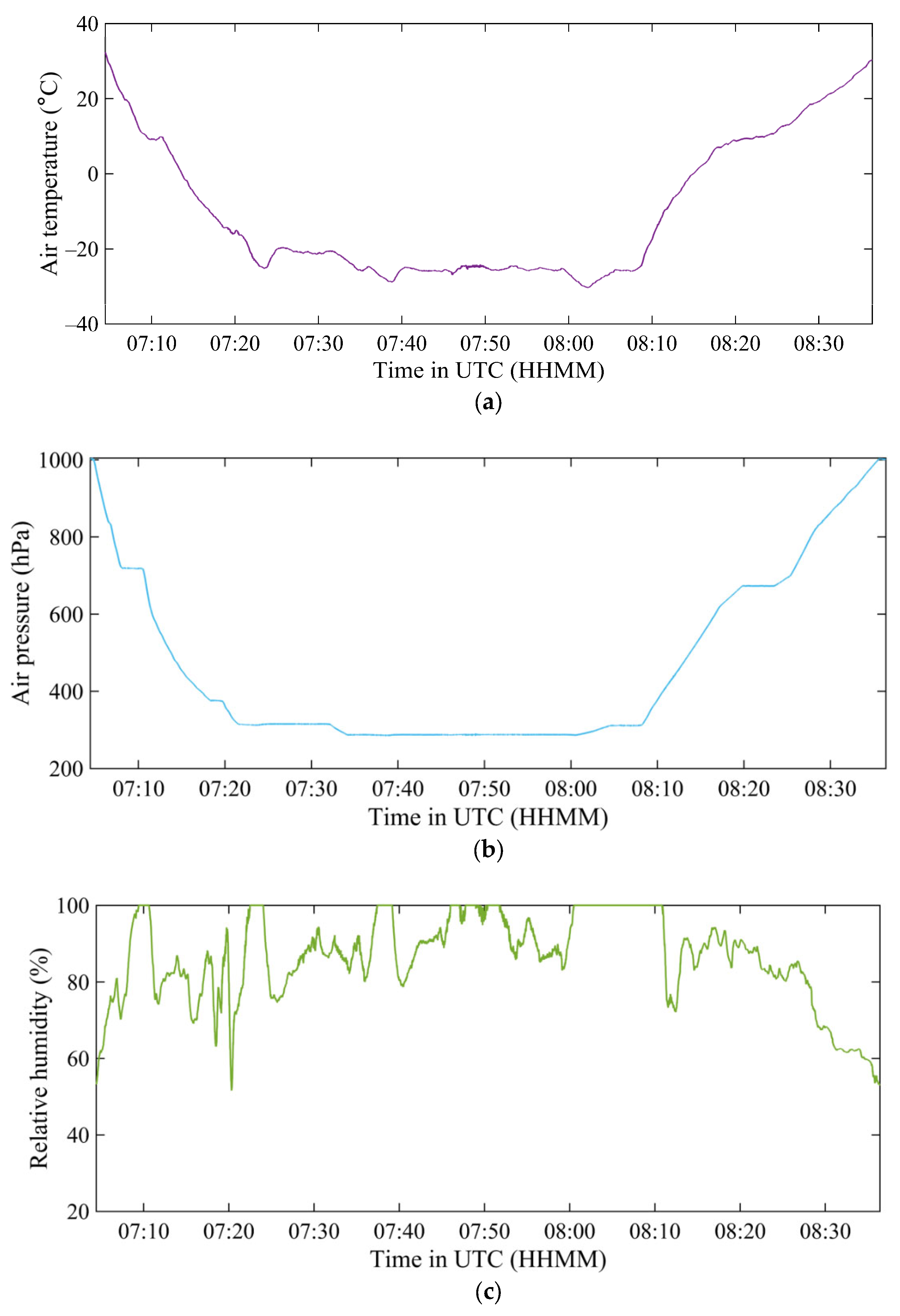
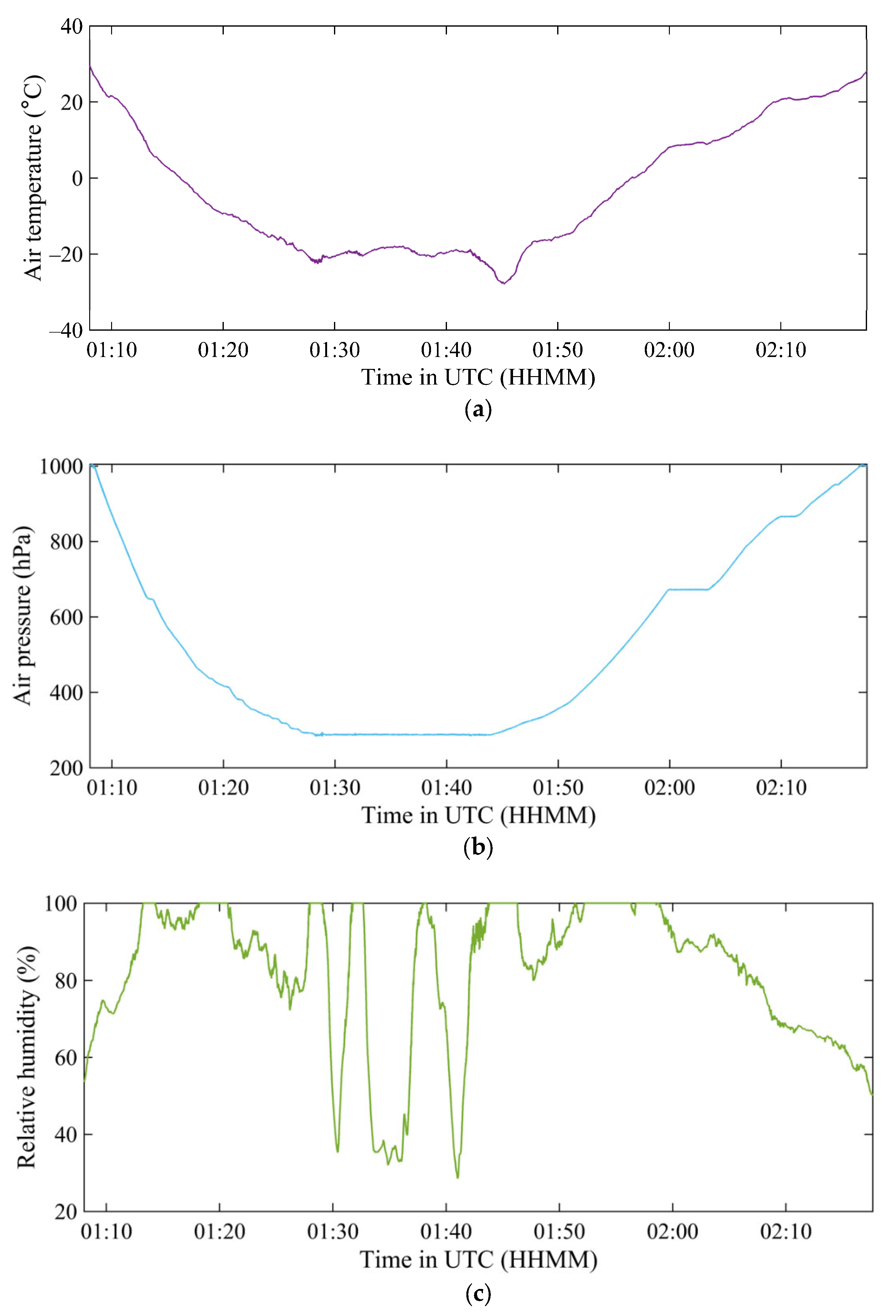
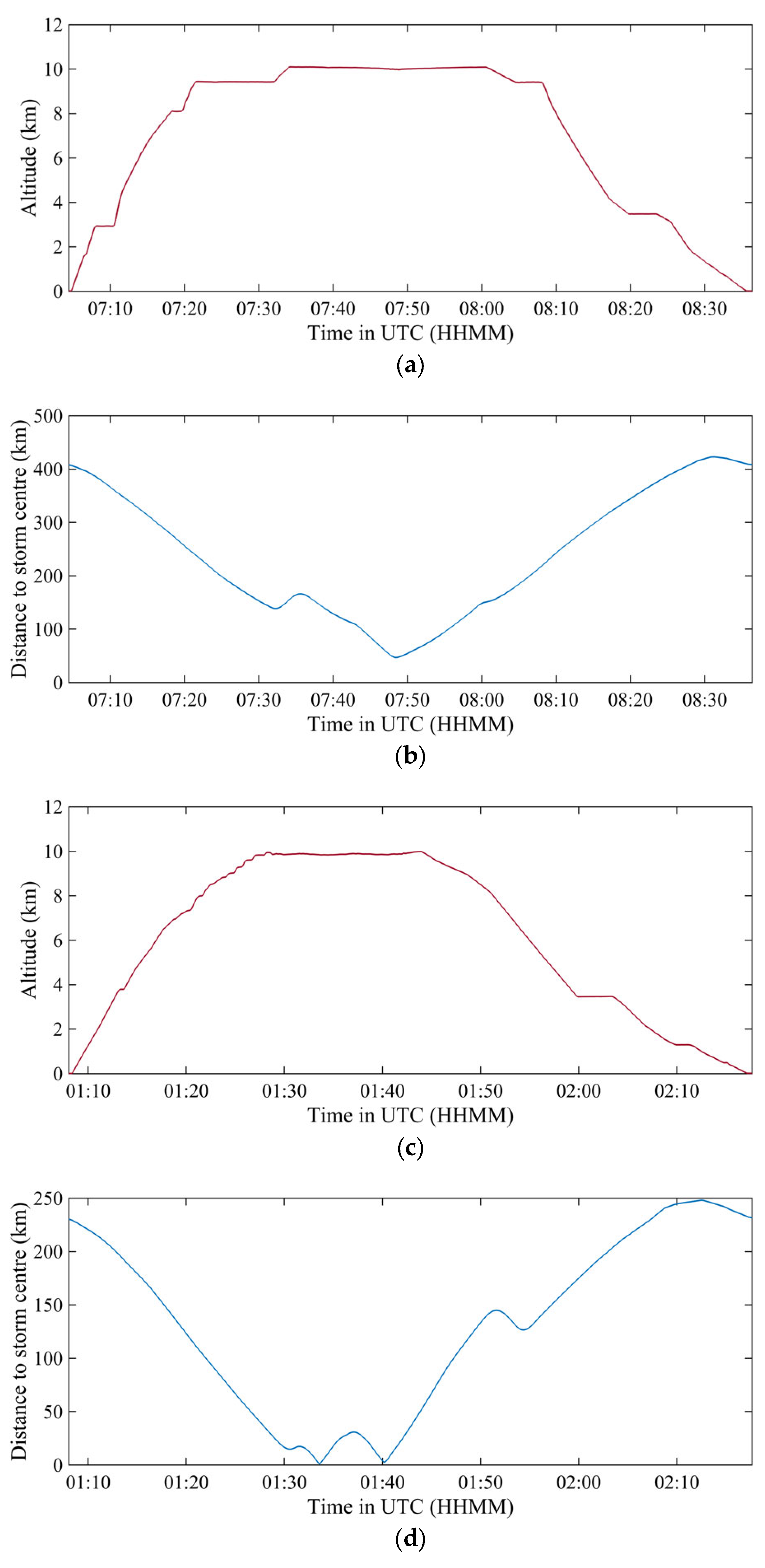
2. Analysis of Flight Data

The flight data were collected by the Aircraft Integrated Meteorological Measuring System 20 Hz (AIMMS20) installed on the Bae Jetstream 4100 (J41) fixed-wing aircraft of GFS. The system measures three orthogonal components of wind velocity, temperature, relative humidity, and pressure, at a frequency of 20 Hz. A detailed description of the AIMMS20 can be found in [24], and the system setup is reported in [21]. The wind velocity data were corrected for aircraft motion and flow distortion based on a Global Positioning System (GPS) module, an inertial measurement unit (IMU), and a central processing module in the AIMMS20 system [21].

The two flights were conducted between around 07 and 09 UTC, 31 August 2023, and between around 01 and 02 UTC, 1 September 2023, respectively. The wind data output by the AIMMS20 is at 5 Hz and is damped with a 20-point sliding window, and it may be treated as gust. Figure 1 shows some selected horizontal wind data along the flights. It could be seen that both flights had been conducted rather close to the eye of Saola at the respective times. The winds were the strongest when the aircraft was located close to the eyewall of Saola, reaching hurricane force wind (wind barbs coloured orange in Figure 1) while the aircraft reached a height of around 10 km above the sea surface.

In the flight of 1 September, the aircraft had penetrated through the eye of Saola, as shown in Figure 1b. At that time, the pilots had taken some pictures around the typhoon eyes and the associated clouds, as shown in Figure 2. The eye of Saola shows up clearly in these pictures. This was the first time that the eye of a super typhoon had ever been visited by an aircraft over the South China Sea, according to the knowledge of the authors and the news.

The time series of the horizontal wind speed and direction as well as the vertical component of the wind during the two flights are shown in Figure 3 and Figure 4, respectively. For the first flight (Figure 3), the maximum measured wind speed was around 36 m/s and was captured one time only. The vertical component of the wind was mostly positive, i.e., an upward motion. For the second flight (Figure 4), maximum winds of around 40 m/s had been captured a couple of times, with a lower wind speed in between. The horizontal wind direction also went through a full circulation as the aircraft got inside and around the typhoon eye. In the eye region, there are both strong upward and downward motions. The positive vertical velocity (upward motion) reaches about 10 m/s, and the negative vertical velocity (downward motion) reaches about −7 m/s. Within the eye, when the horizontal wind direction went through a circle, the vertical velocity changed from being rather positive (generally 5 m/s or above) to being not so positive/even negative (generally below 5 m/s).

The air temperature, air pressure and relative humidity of the two flights are shown in Figure 5 and Figure 6, respectively. The corresponding altitudes are provided in Figure 7. The temperature and humidity do not show very interesting features. For the relative humidity (Figure 5c), as the aircraft was mostly inside clouds during the first flight, it remained relatively high throughout the flight. On the other hand, the aircraft flew around the eye of Saola during the second flight, so that the relative humidity (Figure 6c) showed significant fluctuations and could reach around 30% in the relatively clear region within the eye.

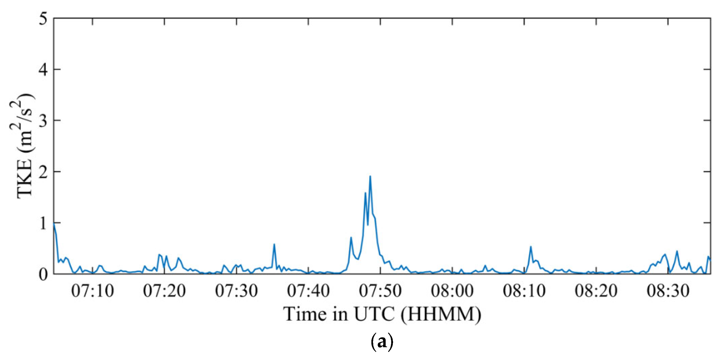
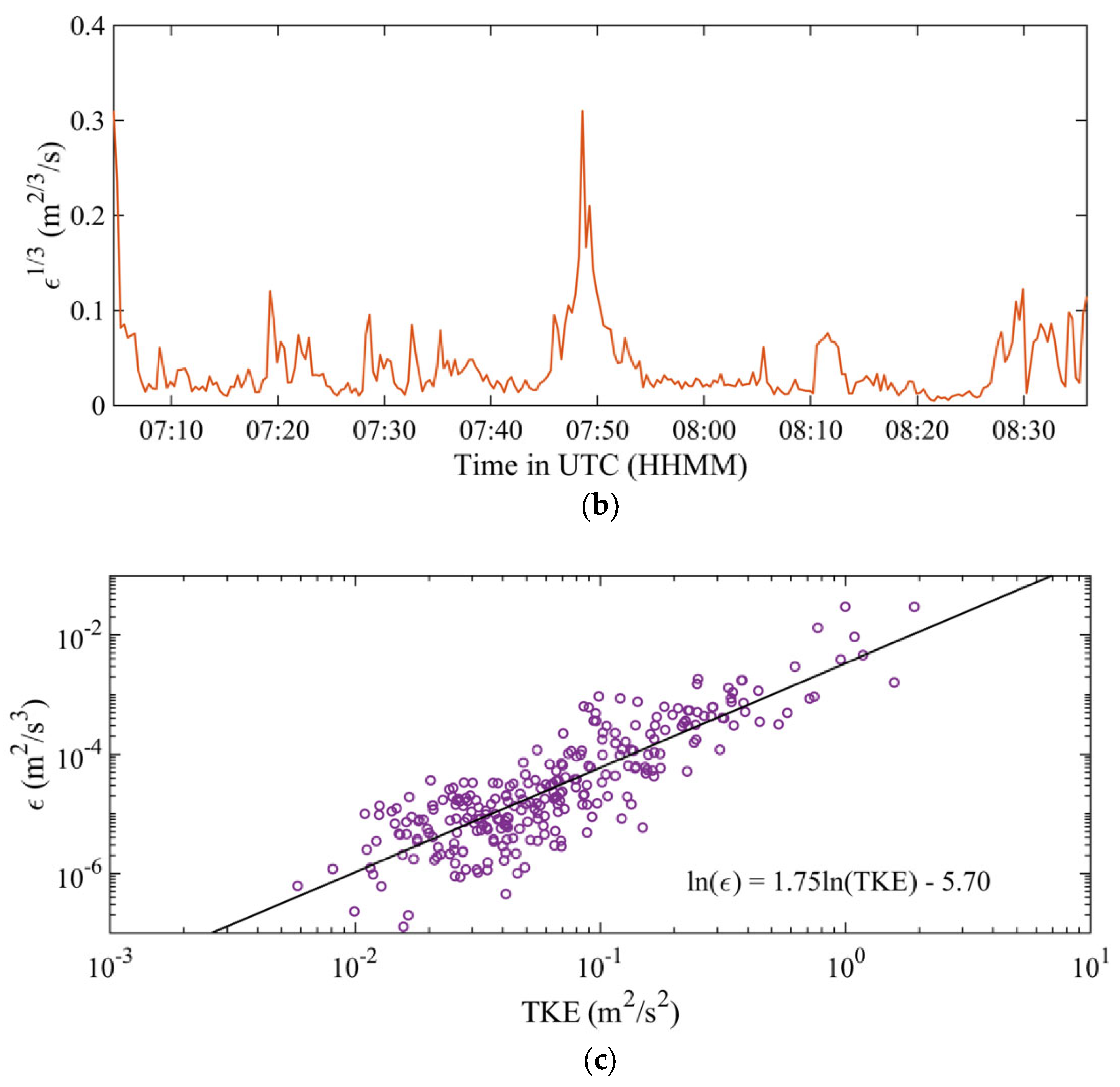
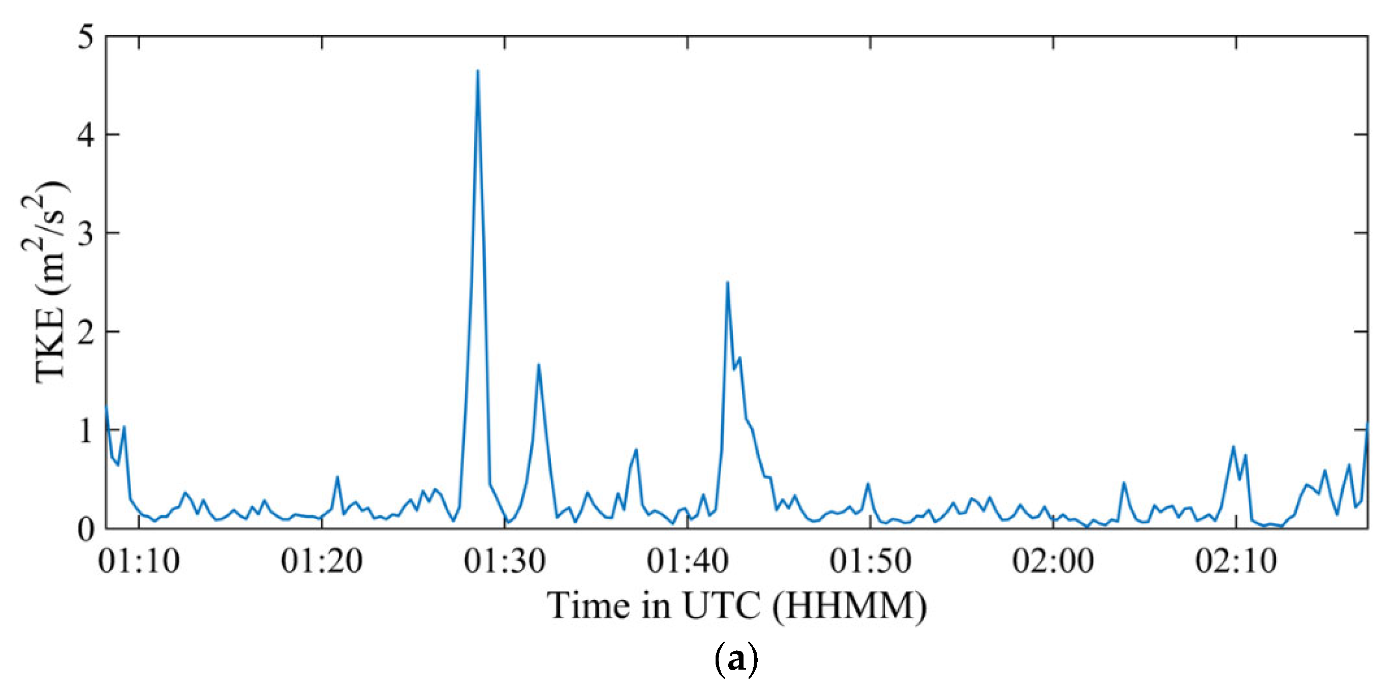
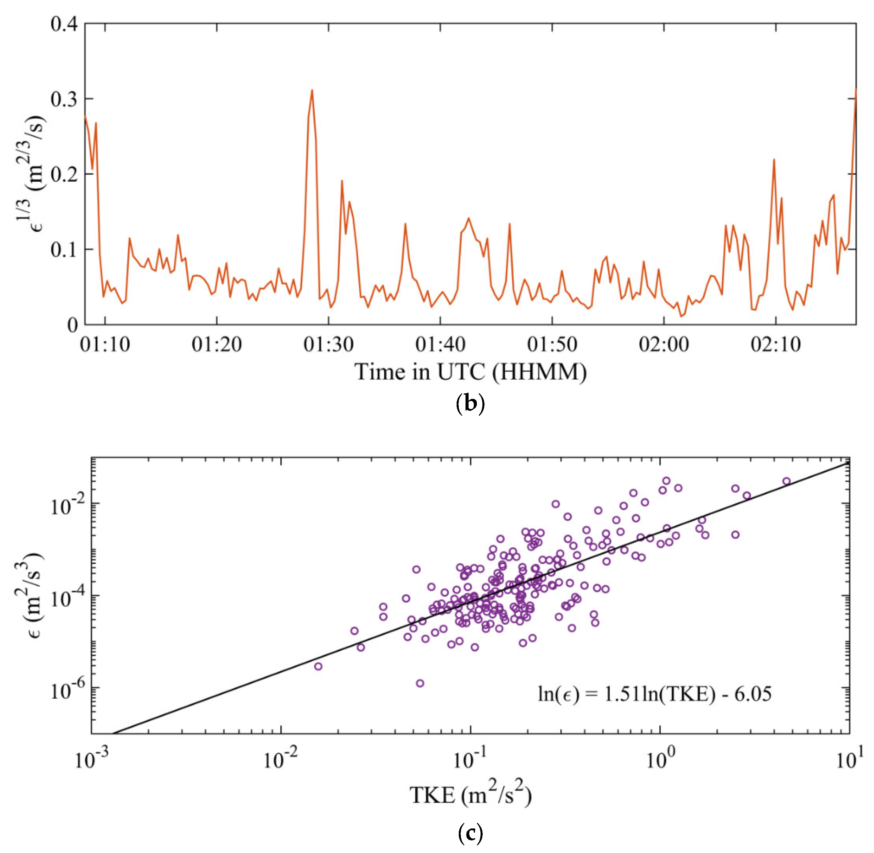
3. Eddy Dissipation Rate and Turbulent Kinetic Energy

The estimation of the turbulent kinetic energy (TKE) and eddy dissipation rate (EDR, ε) follows the procedures described in [12,18], etc. Turbulent fluctuations are extracted by detrending the three orthogonal components of wind velocity in a least-squares manner. A high-pass filter with a cut-off frequency of 0.01 Hz was employed before the detrending. Based on the turbulent fluctuations, the TKE (per unit mass) is calculated as:

$$TKE=\frac{1}{2}\left({\sigma }_u^2+{\sigma }_v^2+{\sigma }_w^2\right)$$

(1)

where σ_u, σ_v, and σ_w are the standard deviations of along-wind, cross-wind, and vertical wind velocity components. Following [12,18], the EDR can be estimated based on the power spectral density of the along-wind velocity component in the inertial subrange:

$$\epsilon ={\alpha }_u{}^{-3/2}\frac{2\pi n}{U_a}{\left[n{S}_u\left(n\right)\right]}^{3/2}$$

(2)

where α_u is the Kolmogorov constant for the along-wind velocity component taken as 0.5 [25], U_a is the true air speed, and S_u(n) is the along-wind velocity spectrum at the frequency n, which should be located within the inertial subrange. Generally, for the flight data analysed here, the inertial subrange with a slope close to −5/3 covers 0.4–4 Hz, and therefore the EDR is estimated based on the wind spectrum over this frequency range.

The TKE and EDR are shown in Figure 8 and Figure 9, respectively, for the two flights. For the first flight (Figure 8), there was a single peak with EDR reaching about 0.3 when the aircraft was close to the typhoon eye. For the second eye (Figure 9), the EDR was generally higher when the aircraft was located at the eyewall or within the eye. It was generally in the order of 0.1 to 0.3.

The local closure techniques are widely used for turbulence parameterisation in numerical weather models [26]. For a local 1.5-order closure, ε can be parameterised as a function of TKE^1.5 [27], or equivalently, there is a relationship between ln(ε) and ln(TKE) with a slope of 1.5. Such a relationship is also widely reported in observational studies, e.g., in [28]. Chan et al. [21], based on aircraft observations in TCs, also showed that the slope between ln(ε) and ln(TKE) is close to 1.5. The TKE and EDR from the two flights have been plotted together in scattered plots, and the results are shown in Figure 8c and Figure 9c. In general, they show good correlations, and the best fit straight lines are shown in these figures. For the 31 August and 1 September cases, the linear regression slopes between ln(ε) and ln(TKE) are 1.75 and 1.51, respectively, which are close to the predicted slope of 1.5 by the local 1.5-order closure parameterisation and agree with the previous observations.

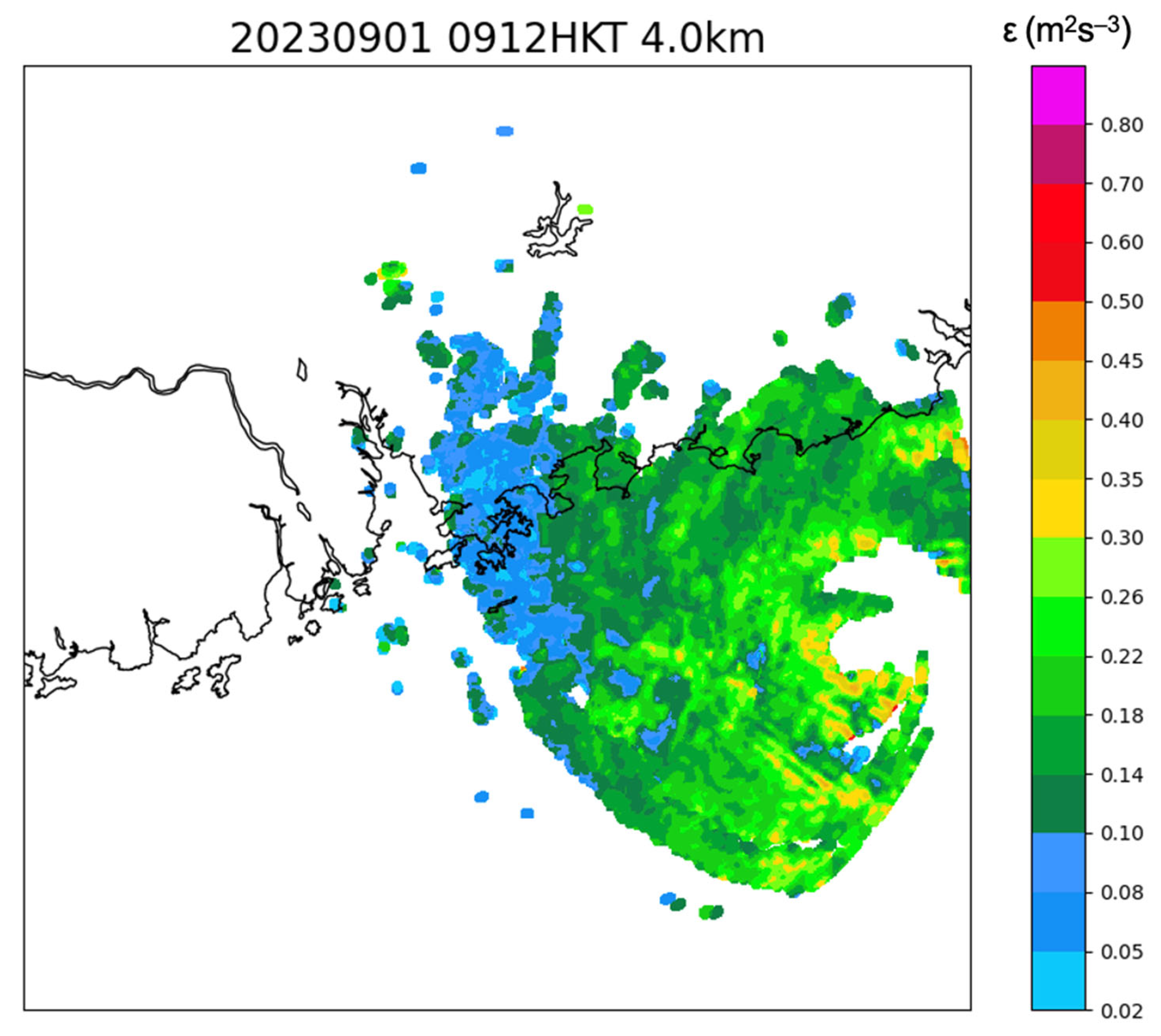
4. EDR Comparison with Radar, Satellite and Model Data

EDR has been estimated from the spectral widths of the weather radars over southern China, based on the methods described in [29]. Such data are only available when Saola was close to the weather radars, and so the results at the time of the second flight are shown in Figure 10. Only EDR data at 1, 2, 3 and 4 km above sea level are available. Figure 10 shows the results from a 4 km height. At that time, the aircraft recorded EDR at around 0.1, which is consistent with the estimation from the radar. This is the first time that the weather-radar-based EDR could be verified using aircraft data in a typhoon situation.

An estimate of the turbulence intensity could also be made based on the gravity waves, as captured by the water vapour channel of the geostationary meteorological satellites. Some background information on the methodology could be found in [30]. Such turbulence intensities are available in real time in HKO, and their spatial distributions around Saola at about the times of the two flights are shown in Figure 11. Gravity waves clearly show up from the analysis of the water vapour satellite pictures. The turbulence intensity is estimated to be of a “moderate” class, which is coloured yellow in Figure 11. This result is consistent with the EDR measurements of 0.3 from the aircraft data.

Turbulence intensity is also estimated from NWP models. HKO uses the method as suggested in [31], and the NWP-based turbulence maps are generated in real time. Examples of the maps at the times of the two flights are shown in Figure 12. Again, moderate turbulence is estimated at the pressure level of 300 hPa, which is around the height of the aircraft when it was close to the typhoon eyes. Again, the NWP-based estimates are consistent with the actual observations from the aircraft.

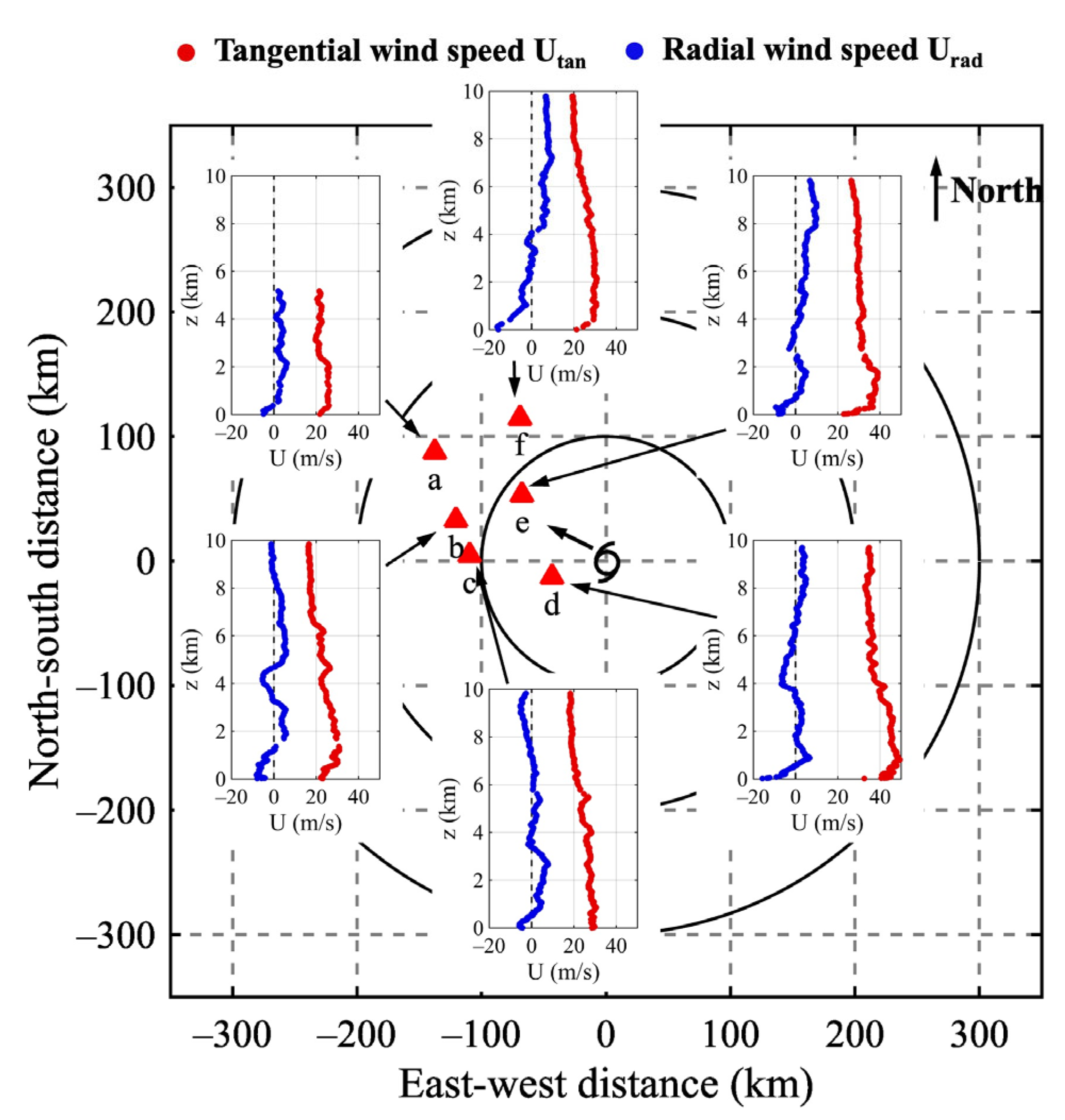
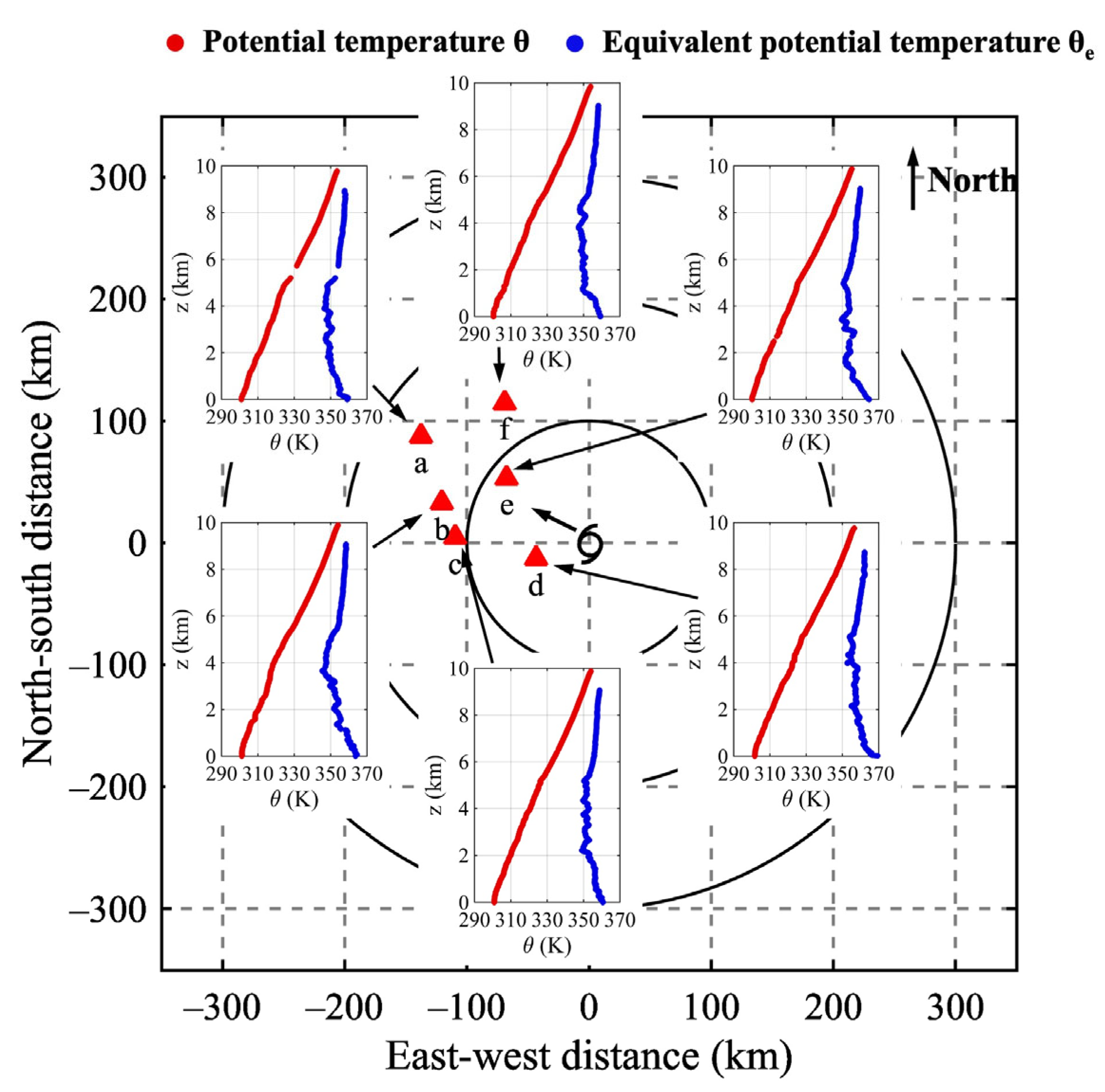
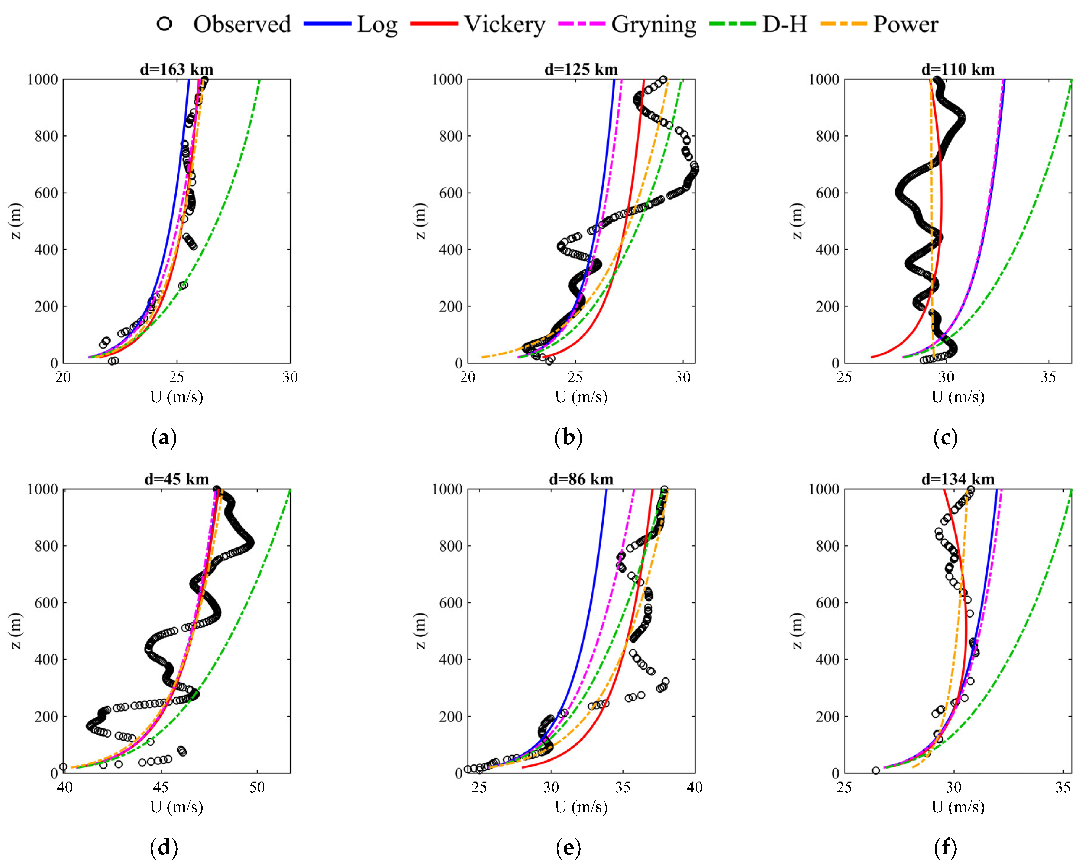
5. Dropsonde Observation

Dropsondes were deployed by the aircraft at an altitude of 10 km. During their descent from 10 km to the sea surface, they collect continuous measurements of vertical profiles of wind speed and direction at a frequency of 4 Hz, along with temperature, humidity, and pressure at a frequency of 2 Hz. Typically, a dropsonde completes its descent in less than 15 min. An overview of the GPS dropsonde dataset can be found in [3], and a detailed description of the dropsonde measurements by the HKO can be found in, e.g., [23,32]. The dropsonde data were quality-controlled using the ASPEN software (Version 3.4.5.) with the Editsonde configuration following [6,33].

Dropsonde data are available in the first flight only. The vertical profiles of inflow and equivalent potential temperatures are shown in Figure 13 and Figure 14, respectively. It could be seen that the atmospheric boundary layer, i.e., below around 1 km, was mostly inflow from the sondes. The heights of the maximum wind speed are also generally around 1 km, which is close to or slightly lower than the inflow layer height. This is consistent with the previous observations of TC boundary layer height scales [1]. The equivalent potential temperature profiles also showed an unstable boundary layer. As such, Saola remained a rather strong system as it moved towards the south China coast. This is consistent with the results, e.g., in [34].

The vertical wind profiles in the boundary layer of the TC, i.e., the first 1 km or so above the sea level, are shown in Figure 15. For the sonde that is closest to the typhoon eye, wind speeds as high as 40 m/s had been recorded. Various wind profile models, including the logarithmic law, the Vickery et al. [35] model, the Gryning et al. [36] model, the Deaves and Harris [11] model, and the power law, were used to fit the observed wind profiles in a least-squares manner. In general, the Vickery model and power-law model provide a better fit to the vertical wind profiles than the other models. It is noted that in previous studies (e.g., [37,38]), the Vickery model usually outperformed the simple power law in describing the “supergradient” flow or low-level jet in the tropical cyclone boundary layer. However, this is not the case here. A more comprehensive and quantitative analysis is warranted based on a larger set of dropsonde data.

6. Conclusions

TC reconnaissance flights had been conducted for Super Typhoon Saola over the northern part of the South China Sea. The flight data provided some insights into the structure of the TC. The general structure of the TC, e.g., maximum wind speed of up to 40 m/s near the eyewall and low wind speed within the eye, low relative humidity within the eye, near-surface inflow in the lowest 1 km, and unstable boundary layer, were captured by the aircraft and dropsonde observations. Updrafts of up to 10 m/s and downdrafts of up to 7 m/s were observed near the eyewall.

Turbulence was also measured during the flights. In particular, EDR and TKE data are available. There is stronger turbulence in terms of TKE and EDR in/near the eyewall of the TC than the other parts. This is consistent with previous observations. The EDR is generally proportional to the TKE raised to the power of approximately 1.5, which agrees with the 1.5-order turbulence parameterisation. The values of EDR from in situ aircraft observations are consistent with the other observations/NWP-based outputs. This is a new finding for super typhoons in the region.

More aircraft data will be collected in the future. Additionally, a database of typhoon observations, particularly for winds, could be built up for this part of the world. Turbulence intensity would be a major subject for such a study.

References

1. Aberson, S.D.; Black, M.L.; Black, R.A.; Burpee, R.W.; Cione, J.J.; Landsea, C.W.; Marks, F.D., Jr. Thirty years of tropical cyclone research with the NOAA P-3 aircraft. Bull. Am. Meteorol. Soc. 2006, 87, 1039–1055. [Google Scholar] [CrossRef]
2. Hock, T.F.; Franklin, J.L. The NCAR GPS dropwindsonde. Bull. Am. Meteorol. Soc. 1999, 80, 407–420. [Google Scholar] [CrossRef]
3. Wang, J.; Young, K.; Hock, T.; Lauritsen, D.; Behringer, D.; Black, M.; Black, P.G.; Franklin, J.; Halverson, J.; Molinari, J.; et al. A long-term, high-quality, high-vertical-resolution GPS Dropsonde dataset for hurricane and other studies. Bull. Am. Meteorol. Soc. 2015, 96, 961–973. [Google Scholar] [CrossRef]
4. Kepert, J.D. Observed boundary layer wind structure and balance in the hurricane core. Part I: Hurricane Georges. J. Atmos. Sci. 2006, 63, 2169–2193. [Google Scholar] [CrossRef]
5. Kepert, J.D. Observed boundary layer wind structure and balance in the hurricane core. Part II: Hurricane Mitch. J. Atmos. Sci. 2006, 63, 2194–2211. [Google Scholar] [CrossRef]
6. Stern, D.P.; Bryan, G.H.; Aberson, S.D. Extreme low-level updrafts and wind speeds measured by dropsondes in tropical cyclones. Mon. Weather Rev. 2016, 144, 2177–2204. [Google Scholar] [CrossRef]
7. Franklin, J.L.; Black, M.L.; Valde, K. GPS dropwindsonde wind profiles in hurricanes and their operational implications. Weather Forecast. 2003, 18, 32–44. [Google Scholar] [CrossRef]
8. Giammanco, I.M.; Schroeder, J.L.; Powell, M.D. GPS dropwindsonde and WSR-88D observations of tropical cyclone vertical wind profiles and their characteristics. Weather Forecast. 2013, 28, 77–99. [Google Scholar] [CrossRef]
9. Powell, M.D.; Vickery, P.J.; Reinhold, T.A. Reduced drag coefficient for high wind speeds in tropical cyclones. Nature 2003, 402, 279–283. [Google Scholar] [CrossRef]
10. French, J.R.; Drennan, W.M.; Zhang, J.A.; Black, P.G. Turbulent fluxes in the hurricane boundary layer. Part I: Momentum flux. J. Atmos. Sci. 2007, 64, 1089–1102. [Google Scholar] [CrossRef]
11. Drennan, W.M.; Zhang, J.A.; French, J.R.; McCormick, C.; Black, P.G. Turbulent fluxes in the hurricane boundary layer. Part II: Latent heat flux. J. Atmos. Sci. 2007, 64, 1103–1115. [Google Scholar] [CrossRef]
12. Zhang, J.A.; Marks, F.D.; Montgomery, M.T.; Lorsolo, S. An estimation of turbulent characteristics in the low-level region of intense hurricanes Allen (1980) and Hugo (1989). Mon. Weather Rev. 2011, 139, 1447–1462. [Google Scholar] [CrossRef]
13. Zhang, J.A. Estimation of dissipative heating using low-level in situ aircraft observations in the hurricane boundary layer. J. Atmos. Sci. 2010, 67, 1853–1862. [Google Scholar] [CrossRef]
14. Zhang, J.A. Spectral characteristics of turbulence in the hurricane boundary layer over the ocean between the outer rain bands. Q. J. R. Meteorol. Soc. 2010, 136, 918–926. [Google Scholar] [CrossRef]
15. Zhang, J.A.; Drennan, W.M. An observational study of vertical eddy diffusivity in the hurricane boundary layer. J. Atmos. Sci. 2012, 69, 3223–3236. [Google Scholar] [CrossRef]
16. Zhang, J.A.; Montgomery, M.T. Observational estimates of the horizontal eddy diffusivity and mixing length in the low-level region of intense hurricanes. J. Atmos. Sci. 2012, 69, 1306–1316. [Google Scholar] [CrossRef]
17. Zhao, Z.; Chan, P.W.; Wu, N.; Zhang, J.A.; Hon, K.K. Aircraft observations of turbulence characteristics in the tropical cyclone boundary layer. Bound.-Layer Meteorol. 2019, 174, 493–511. [Google Scholar] [CrossRef]
18. Sparks, N.; Hon, K.K.; Chan, P.W.; Wang, S.; Chan, J.C.L.; Lee, T.C.; Toumi, R. Aircraft observations of tropical cyclone boundary layer turbulence over the South China Sea. J. Atmos. Sci. 2019, 76, 3773–3783. [Google Scholar] [CrossRef]
19. Gopalakrishnan, S.; Hazelton, A.; Zhang, J.A. Improving hurricane boundary layer parameterization scheme based on observations. Earth Space Sci. 2021, 8, e2020EA001422. [Google Scholar] [CrossRef]
20. Hon, K.K.; Chan, P.W. A decade (2011–2020) of tropical cyclone reconnaissance flights over the South China Sea. Weather 2022, 77, 308–314. [Google Scholar] [CrossRef]
21. Chan, P.W.; Hon, K.K.; Foster, S. Wind data collected by a fixed-wing aircraft in the vicinity of a tropical cyclone over the south China coastal waters. Meteorol. Z. 2011, 20, 313–321. [Google Scholar] [CrossRef]
22. Chan, P.W.; Wong, W.K.; Hon, K.K. Weather observations by aircraft reconnaissance inside Severe Typhoon Utor. Weather 2014, 69, 199–203. [Google Scholar] [CrossRef]
23. Chan, P.W.; Wu, N.G.; Zhang, C.Z.; Deng, W.J.; Hon, K.K. The first complete dropsonde observation of a tropical cyclone over the South China Sea by the Hong Kong Observatory. Weather 2018, 73, 227–234. [Google Scholar] [CrossRef]
24. Beswick, K.M.; Gallagher, M.W.; Webb, A.R.; Norton, E.G.; Perry, F. Application of the Aventech AIMMS20AQ airborne probe for turbulence measurements during the Convective Storm Initiation Project. Atmos. Chem. Phys. 2008, 8, 5449–5463. [Google Scholar] [CrossRef]
25. Sreenivasan, K.R. On the universality of the Kolmogorov constant. Phys. Fluids 1995, 7, 2778–2784. [Google Scholar] [CrossRef]
26. Mellor, G.L.; Yamada, T. A hierarchy of turbulence closure models for planetary boundary layers. J. Atmos. Sci. 1974, 31, 1791–1806. [Google Scholar] [CrossRef]
27. Stull, R.B. An Introduction to Boundary Layer Meteorology, 1st ed.; Springer: Berlin/Heidelberg, Germany, 1988. [Google Scholar]
28. Vecenaj, Z.; Belusic, D.; Grisogono, B. Characteristics of the near-surface turbulence during a bora event. Ann. Geophys. 2010, 28, 155–163. [Google Scholar] [CrossRef]
29. Chan, P.W.; Zhang, Y.; Doviak, R.J. Calculation and application of eddy dissipation rate map based on spectrum width data of a S-band radar in Hong Kong. MAUSAM 2016, 67, 411–422. [Google Scholar] [CrossRef]
30. Wimmers, A.; Griffin, S.; Gerth, J.; Bachmeier, S.; Lindstrom, S. Observations of gravity waves with high-pass filtering in the new generation of geostationary imagers and their relation to aircraft turbulence. Weather Forecast. 2018, 33, 139–144. [Google Scholar] [CrossRef]
31. Kwok, J.L.; Chan, H.T.; Yin, P.W.; Li, C.Y.Y. Automatic aviation turbulence detection using advanced machine learning techniques. In Proceedings of the AOGS2022, Singapore, 1–5 August 2022; Asia Oceania Geosciences Society (AOGS): Singapore, 2022. [Google Scholar]
32. He, J.Y.; Hon, K.K.; Li, Q.S.; Chan, P.W. Wind profile analysis for selected tropical cyclones over the South China Sea based on dropsonde measurements. Atmósfera 2022, 35, 111–126. [Google Scholar] [CrossRef]
33. Zhang, J.A.; Rogers, R.F.; Reasor, P.D.; Uhlhorn, E.W.; Marks, F.D. Asymmetric hurricane boundary layer structure from dropsonde composites in relation to the environmental vertical wind shear. Mon. Weather Rev. 2013, 141, 3968–3984. [Google Scholar] [CrossRef]
34. He, J.Y.; Hon, K.K.; Chan, P.W.; Li, Q.S. Dropsonde observations and numerical simulations for intensifying and weakening tropical cyclones over the northern part of the South China Sea. Weather 2022, 77, 332–338. [Google Scholar] [CrossRef]
35. Vickery, P.J.; Wadhera, D.; Powell, M.D.; Chen, Y. A hurricane boundary layer and wind field model for use in engineering applications. J. Appl. Meteorol. Climatol. 2009, 48, 381–405. [Google Scholar] [CrossRef]
36. Gryning, S.E.; Batchvarova, E.; Brümmer, B.; Jørgensen, H.; Larsen, S. On the extension of the wind profile over homogeneous terrain beyond the surface boundary layer. Bound.-Layer Meteorol. 2007, 124, 251–268. [Google Scholar] [CrossRef]
37. Chan, P.W.; Choy, C.W.; Mak, B.; He, J.Y. A rare tropical cyclone necessitating the issuance of gale or storm wind warning signal in Hong Kong in late autumn in 2022—Severe Tropical Storm Nalgae. Atmosphere 2023, 14, 170. [Google Scholar] [CrossRef]
38. He, J.Y.; Li, Q.S.; Chan, P.W.; Choy, C.W.; Mak, B.; Lam, C.C.; Luo, H.Y. An observational study of Typhoon Talim over the northern part of the South China Sea in July 2023. Atmosphere 2023, 14, 1340. [Google Scholar] [CrossRef]
Figure 1. Flight routes and horizontal wind data along the flights overlaid on false colour imagery generated from Himawari-9 geostationary satellite of Japan Meteorological Agency, (a) flight between around 07 and 09 UTC, 31 August 2023 on top of satellite data at 08 UTC; (b) flight between around 01 and 02 UTC, 1 September 2023 on top of satellite data at 02 UTC.
Atmosphere 14 01595 g001
Figure 2. Photos around the typhoon eyes and the associated clouds taken during the eyewall penetration on 1 September 2023.
Atmosphere 14 01595 g002
Figure 3. Time series of the instantaneous (a) horizontal wind speed, (b) wind direction, and (c) vertical wind speed based on the aircraft data on 31 August 2023.
Atmosphere 14 01595 g003
Figure 4. Time series of the instantaneous (a) horizontal wind speed, (b) wind direction, and (c) vertical wind speed based on the aircraft data on 1 September 2023.
Atmosphere 14 01595 g004
Figure 5. Time series of the (a) temperature, (b) pressure, and (c) relative humidity based on the aircraft data on 31 August 2023.
Atmosphere 14 01595 g005
Figure 6. Time series of the (a) temperature, (b) pressure, and (c) relative humidity based on the aircraft data on 1 September 2023.
Atmosphere 14 01595 g006
Figure 7. Time series of the flight altitude and distance to storm centre on (a,b) 31 August 2023 and (c,d) 1 September 2023.
Atmosphere 14 01595 g007
Figure 8. (a) Time series of the turbulent kinetic energy (TKE) based on the aircraft data on 31 August 2023, (b) time series of the cube root of the eddy dissipation rate (ε1/3), and (c) variation of ε with TKE. The black line in (c) represents the linear fit between ln(ε) and ln(TKE).
Atmosphere 14 01595 g008aAtmosphere 14 01595 g008b
Figure 9. (a) Time series of the turbulent kinetic energy (TKE) based on the aircraft data on 1 September 2023, (b) time series of the cube root of the eddy dissipation rate (ε1/3), and (c) variation of ε with TKE. The black line in (c) represents the linear fit between ln(ε) and ln(TKE).
Atmosphere 14 01595 g009aAtmosphere 14 01595 g009b
Figure 10. Composite Eddy Dissipation Rate (EDR) map (in units of m2/s3) derived from spectrum width data measured by the Tate’s Cairn Weather Radar in Hong Kong and Zhu Ao Weather Radar in Zhuhai at 4 km height above sea level at 01:12 UTC on 1 September 2023.
Atmosphere 14 01595 g010
Figure 11. Gravity waves as captured by water vapour channel of the geostationary meteorological satellites. The turbulence intensity estimated to be of “moderate” class is coloured yellow.
Atmosphere 14 01595 g011aAtmosphere 14 01595 g011b
Figure 12. Turbulence intensity estimated from the NWP model.
Atmosphere 14 01595 g012aAtmosphere 14 01595 g012b
Figure 13. Vertical profiles of instantaneous tangential (red) and radial (blue) wind speeds in Typhoon Saola at around 0800 UTC 31 August 2023. Tangential wind speed: anti-clockwise positive; radial wind speed: outflow positive. Red triangles represent dropsonde locations relative to the storm centre.
Atmosphere 14 01595 g013
Figure 14. Vertical profiles of potential temperature (red) and equivalent potential temperature (blue) in Typhoon Saola at around 0800 UTC 31 August 2023. Red triangles represent dropsonde locations relative to the storm centre.
Atmosphere 14 01595 g014
Figure 15. Fitting of vertical profiles of instantaneous wind speeds in the lowest 1000 m in Typhoon Saola to the wind profile models, including the logarithmic law, Vickery model, Gryning model, Deaves and Harris model, and power law. d represents the distance to the storm centre.
Atmosphere 14 01595 g015
Disclaimer/Publisher’s Note: The statements, opinions and data contained in all publications are solely those of the individual author(s) and contributor(s) and not of MDPI and/or the editor(s). MDPI and/or the editor(s) disclaim responsibility for any injury to people or property resulting from any ideas, methods, instructions or products referred to in the content.