Article

The Interrelated Pollution Characteristics of Atmospheric Speciated Mercury and Water-Soluble Inorganic Ions in Ningbo, China

1
Center for Excellence in Regional Atmospheric Environment & Fujian Key Laboratory of Atmospheric Ozone Pollution Prevention & Key Laboratory of Urban Environment and Health, Institute of Urban Environment, Chinese Academy of Sciences, Xiamen 361021, China
2
University of Chinese Academy of Sciences, Beijing 100049, China
3
Zhejiang Key Laboratory of Urban Environmental Process and Pollution Control, Ningbo (Beilun) Zhongke Haixi Industrial Technology Innovation Center, Ningbo 315800, China
4
School of Chemistry and Environmental Engineering, Hanshan Normal University, Chaozhou 521041, China
*
Authors to whom correspondence should be addressed.
These authors contributed equally to this work.
Atmosphere 2023, 14(11), 1594; https://doi.org/10.3390/atmos14111594
Submission received: 21 August 2023 / Revised: 12 October 2023 / Accepted: 20 October 2023 / Published: 24 October 2023
(This article belongs to the Special Issue Air Pollution in Asia)

Abstract

:
Atmospheric mercury and water-soluble inorganic ions (WSIIs) are commonly observable airborne pollutants in the atmosphere that may have similar emission sources. In this study, the interrelated pollution characteristics of atmospheric speciated mercury and WSIIs were studied using a Piper diagram, correlation analysis, pollution episode analysis and potential source contribution function (PSCF) techniques. Also, an empirical regression equation for predicting the temporal variation in gaseous elemental mercury (GEM) was constructed. The results showed that the concentrations of GEM and particle-bound mercury (PBM) roughly increased with the increasing percentage values of NH4+ in cationic normality, and exponentially increased with the decreasing percentage values of Na+ + Mg2+ in cationic normality. Correlation analysis revealed that the atmospheric speciated mercury was positively (p < 0.01) correlated with most water-soluble inorganic ions, especially for GEM, which was closely correlated with NO2, NOx, CO, PM2.5, NO3 SO42−, NH4+ and K+ (r > 0.5, p < 0.01), indicating that the emission sources of GEM were related to fossil fuel and biomass combustion, industrial activities, and traffic exhausts. Pollution episode analysis showed that PM2.5, WSIIs (including SO42−, NO3, NH4+, K+ and Cl), SO2 and NO2 generally exhibited synchronous variations with GEM and PBM, and positive correlations were observed between GEM and PM2.5, SO42−, NO3, NH4+, K+, Cl, SO2 and NO2 (r = 0.35–0.74, p-value < 0.01). In addition, the potential source region of GEM was similar to that of PM2.5, SO42−, NO3, NH4+, K+ and Ca2+. Based on the above findings, a satisfactory empirical regression equation, with PM2.5, NOx, CO and the percentage value of Na+ + Mg2+ in cationic normality as independent variables for GEM simulation, was constructed. The result showed that the variation in GEM concentrations could be predicted well by these variables. This model could serve as a potential substitute tool for GEM measurement in the future.

1. Introduction

Due to rapid industrialization and urbanization, air pollution remains a severe environmental problem in China [1]. In particular, atmospheric mercury, which is characterized as having persistent bioaccumulative and neurotoxic properties, has gradually become a major potential hazard to human health. It is capable of entering human bodies through the respiratory tract and causing damage to human organs, manifesting in gastrointestinal ulcers, diarrhea, pulmonary edema, respiratory failure, and neuropsychiatric symptoms [2]. In the atmosphere, mercury is operationally defined into three types of species: elemental mercury (GEM), gaseous oxidized mercury (GOM) and particle-bound mercury (PBM, i.e., mercury associated with particles with sizes ≤2.5 μm). These are emitted from anthropogenic or natural sources and are widely distributed in the troposphere [3].
The study of the interaction between atmospheric mercury and conventional air pollutants is an interesting field, and has been gradually recognized by the academic community in recent decades. Previous studies have reported that some photochemical oxidants such as O3, OH and reactive halogens (Br, BrO, Cl, et al.) are capable of oxidizing GEM to GOM during the daytime [4,5]. In contrast, the aqueous-phase reduction of GOM to GEM by some reductants (such as organic acid, iron and SO32−) is an important sink for GOM [6,7,8,9]. GEM and GOM are the species present in the gas phase of the atmosphere. These species can undergo transformation into the solid phase (i.e., PBM) through processes such as gas–particle partitioning or particle adsorption. Previous studies have shown that the composition of aerosol particles plays an important role in influencing these transformation processes [10,11].
Many studies have revealed that the concentration of GEM is relatively low in remote background sites in the Northern Hemisphere (1.50~1.70 ng m−3) and rural sites in Asia, Europe, and North America (1.1~2.0 ng m−3) [12,13,14,15,16,17]. However, higher levels have been observed in Asian urban and suburban areas, such as Shanghai (4.2 ng m−3), Xiamen (3.5 ng m−3), Guiyang (9.7 ng m−3), and Seoul (3.2 ng m−3) [7,18,19,20]. Generally, high levels of atmospheric speciated mercury are mainly impacted by anthropogenic emissions such as coal combustion, non-ferrous smelting, and vehicle exhausts [21]. These emission sources also account for the pollution of conventional pollutants in the atmosphere. This results in some reported linear or nonlinear relationships between atmospheric mercury and conventional pollutants, especially in mainland China [7,22,23,24]. For example, the total gaseous mercury concentrations (TGM, defined as the sum of GEM and GOM) were found to have strong linear relationships with PM2.5 (r = 0.474, p < 0.01), NO2 (r = 0.421, p < 0.01) and CO (r = 0.414, p < 0.01) during a long-term observation period at a coastal site in Qingdao, China [25]. GEM and PBM were also found to have similar linear relationships with PM2.5 in Ningbo (r = 0.37~0.45, p < 0.05) [26] and Shanghai (r = 0.36~0.72, p value not available) [7], respectively. Among these conventional air pollutants, the particle matter (mainly PM2.5) is an extremely complex species that is composed of many different kinds of organic and inorganic components. It is well known that water-soluble inorganic ions (WSIIs) such as NO3, SO42−, NH4+, Cl, Na+, Mg2+, Ca2+ and K+ are important components of PM2.5, which may have a close inherent connection and similar sources to those of atmospheric mercury. However, few studies have focused on the interrelationship between atmospheric mercury and the eight WSIIs in PM2.5, which is a gap in the investigation of the pollution characteristics of atmospheric mercury.
Currently, several models have provided estimates of the pollution characteristics of atmospheric mercury, such as the Global/Regional Atmospheric Heavy Metals Model (GRAHM), the Global EMEP Multi-media Modelling System (GLEMOS), the Danish Eulerian Hemispheric Model (DEHM), and the Global EMEP Multi-media Modelling System (GEOS-Chem) [27]. These models mainly focus on modeling the distribution, deposition and transformation of atmospheric mercury on a global or regional scale, with long time periods (yearly, monthly or daily); this involves complex meteorological and physical–chemical processes. However, few studies have investigated the atmospheric mercury modeling on an hourly time scale. The close relationships between atmospheric mercury and conventional air pollutants are helpful in modeling the hourly variations in atmospheric mercury, which has significant implications for improving the available global or regional mercury prediction models.
In this study, the speciated mercury, conventional air pollutants and WSIIs were simultaneously monitored, with the trend in the temporal variation and the relationship between atmospheric mercury and WSIIs being investigated during the study period from December 2016 to November 2017. The main objectives were as follows: (1) to investigate the factors influencing the pollution characteristics of atmospheric mercury; (2) to evaluate the intrinsic connection between atmospheric mercury and WSIIs, and (3) to explore the forecasting models for atmospheric mercury within a short time scale. The results of this study can provide useful insights into the potential sources and factors affecting speciated atmospheric mercury. Additionally, the forecasting models for atmospheric mercury developed in this study could contribute to improving existing global or regional mercury prediction models to some extent.

2. Materials and Methods

2.1. Site Description

The observatory site is situated at a coastal site of Beilun district, Ningbo city, in the eastern Yangtze River Delta (YRD) region of China (Figure 1). The YRD region covers an area of approximately 100,000 km2 and has a population of 75 million [1]. As one of the most densely populated and economically developed regions in China, the anthropogenic emissions of mercury in the YRD region were approximately 2.5~2.7 t from 2014 to 2016 [28]. This region may have experienced mercury pollution as a result of emissions from anthropogenic activities. The emissions of SO2, NOX, PM10, PM2.5, NMVOCs and NH3 in the year of 2010 were estimated to be 2147 kt, 2776 kt, 1006 kt, 643 kt, 3822 kt and 1439 kt, respectively [29]. As the typical industrial and harbor city of the YRD, Ningbo has an average annual temperature, sunshine hours and precipitation of 16.4 °C, 1850 h and 1480 mm, respectively. A previous study reported that the concentration of atmospheric mercury in Ningbo city ranges from 0.64 to 13.58 ng m−3, with an annual average of 2.44 ng m−3 [26]. The annual average concentration of PM2.5 was 39.0 μg/m3 in 2016 according to the Report on the State of the Environment in Ningbo. In this study, speciated atmospheric Hg and PM2.5 components were simultaneously measured on the rooftop of the Ningbo Urban Environment Observation and Research Station (NUEORS), Chinese Academy of Sciences (121°53′42.32″ E, 29°45′4.59″ N, 15 m a. s. l., UTC+8). The NUEORS is 37 km southeast of the city center of Ningbo. Several industrial factories are adjacent to the study site, including an automobile factory, a fabric plant, a natural gas processing plant and some mechanical fitting factories. A coal-fired power plant (Beilun coal-fired power plant) is located approximately 20 km northwest of the station. It is the third largest coal-fired power plant in China, with a total installed capacity of 5000 MW.

2.2. Measurement of Atmospheric Mercury Species, WSIIs in PM2.5 and Other Parameters

Speciated atmospheric Hg was continuously measured using a fully automated mercury analyzer (Tekran 2537B, 1135, 1130, Tekran Instruments Corporation, Toronto, ON, Canada) (Figure 1) with a detection limit of 0.10 ng m−3 at a time resolution of 5 min for GEM. Both GOM and PBM have a 1.6 pg m−3 detection limit and 2 h time resolution. The monitored concentration of GOM might be lower than the true values to some extent, due to a systematic bias that exists for this instrument [30]. The concentrations of WSIIs (NO3, SO42−, NH4+, Cl, Na+, Mg2+, Ca2+ and K+) at the study site were synchronously measured using MARGA ADI 2080 (Metrohm AG, Herisau, Switzerland) (Figure 1) with hourly time resolution. MARGA is able to simultaneously measure the precursor gases and aerosol ionic components in ambient air, and it has been used in many studies over Europe and North America. This method has been compared with other reference methods to confirm that it is a reliable technique [31,32]. The detection limits for NO3, SO42−, NH4+, Cl, Na+, Mg2+, Ca2+ and K+ are 0.1, 0.1, 0.1, 0.1, 0.1, 0.1, 0.2 and 0.1 μg m−3, respectively. In this study, conventional air pollutants (NOx, O3, CO, PM10, PM2.5 and SO2) and meteorological parameters were also monitored during the study period. Detailed descriptions of the monitoring instruments and procedural details are given elsewhere [7,32,33].

2.3. Piper Diagram Analysis

Piper diagrams (or Trilinear diagrams) are used as an effective graphical representation of the chemistry of water samples in hydro-geological studies, and can be plotted using OriginPro software. We applied the Piper diagramming method to aerosol research in our previous work [33]. In brief, the major cation and anion proportions (expressed as percentages in cationic or anionic normality, %Meq/m3) were presented in the bottom triangles on the left and right, respectively. The total dissolved ionic contents (also in normality) and the relative percentages of the composition of both cations and anions were projected to the rhombus in the top center of the diagram. The three sub-panels could be divided into a few different regions, indicating different dominant ionic species. By systematically comparing the properties and sources of each ion, the final six ion groups used in the Piper diagram for aerosol analysis were three cation groups (i.e., [Ca2++ K+], [Na++ Mg2+] and [NH4+]) and three anion constituents (i.e., [SO42−], [NO3] and [Cl]). A simple example of a Piper diagram can be seen in Figure S1.

2.4. Backward Trajectory and Potential Source Contribution Function (PSCF) Analyses

Atmospheric GEM, PM2.5 and WSIIs are influenced by local emissions, and by both regional and long-range transportation from the source region. In order to investigate the potential sources of these species, the 72 h air mass backward trajectories arriving at the study site at a 500 m altitude and the potential source contribution function were calculated using the MeteoInfo software (Version: 1.4.9) [34]. The calculated trajectories were converted to the ESRI shape file format, and then the hourly average concentrations of air pollutants were assigned to the corresponding trajectories. Before performing PSCF analysis, a PSCF grid layer with a 0.4° × 0.4° cell size was created. The PSCF values for each grid cell were calculated by counting the trajectory segment endpoints that terminate within each cell (Equation (1)):
PSCFij = mij/nij
where mij is the number of trajectory segment endpoints that fall in the ijth cell and have arrival times at the study site corresponding to pollutant concentrations higher than the average concentration, and nij is the number of endpoints that fall in the same cell.
The calculated PSCF values were multiplied by an arbitrary weight function [7] to reduce the uncertainty of cells, within which the total number of endpoints was less than approximately three times the average value of the end points per each cell.

2.5. Statistical Analysis and Model Construction Processes

In this study, the univariate Kolmogorov–Smirnov (K–S) test was employed to assess the adherence of the data series to a normal distribution. The correlation analysis between the chemical species was conducted using SPSS software (Version 22.0), utilizing hourly concentration data, and the coefficients used were Spearman’s rho. The process of model building was as follows: first, the equation of the multivariate nonlinear model that contains unknown coefficients based on the relationships between the variables was constructed. Then, the optimal coefficients were calculated using the iterative regression function of the Origin 2022 software. Once the model was built, the future period data, which was not used for model building, was adopted to test and evaluate the strengths and weaknesses of the model.

3. Results and Discussion

3.1. Temporal Variations of Speciated Hg, PM2.5 and WSIIs

A summary of the GEM, GOM, PBM, PM2.5 and WSIIs concentrations measured from December 2016 to November 2017 is presented in Table S1. During the entire sampling period, the arithmetic average concentrations of GEM, GOM, PBM and PM2.5 were 2.4 ± 0.9 ng m−3, 99.3 ± 199.5 pg m−3, 286.5 ± 448.0 pg m−3 and 25.1 ± 17.2 μg m−3, respectively, and the median concentrations of these four species were 2.2 ng m−3, 43.5 pg m−3, 130.8 pg m−3 and 20.6 μg m−3, respectively. Table 1 summarizes the results of previous studies on speciated mercury and PM2.5, and indicates that the GEM concentration of the study site in Ningbo was higher than that of the remote background sites in the Northern hemisphere (1.50~1.70 ng m−3) and the rural sites in Asia, Europe and North America (1.1~2.0 ng m−3) [12,13,14,15,16,17]. Meanwhile, the GEM concentration found in this study was lower than the values reported for other Asian urban and suburban areas in Shanghai (4.2 ng m−3), Xiamen (3.5 ng m−3), Guiyang (9.7 ng m−3), and Seoul (3.2 ng m−3) [7,18,19,20]. As for GOM and PBM, the concentrations found in this study were higher than those reported for most other sites (Table 1), except for Taichuang and Guiyang, where the monitoring sites were situated in the urban/industrial region and a mining area, respectively, with large anthropogenic emissions [35]. The high GOM and PBM concentrations observed in this study can be accounted for by the following factors. Firstly, most GOM and PBM come from anthropogenic emission sources, including coal-fired power plants and municipal solid waste incinerators [36]. Ningbo is a highly industrialized city. There are 18 coal-fired power plants, with their total consumption of coal and crude oil being 36.7 and 29.1 million tons, respectively, in 2017 (Statistical Yearbook of Ningbo, 2017). In addition, the third largest coal-fired power plant in China, with a total installed capacity of 5000 MW, is located 22 km away to the northwest of the study site. These anthropogenic sources might release large quantities of GOM and PBM into the atmosphere. Secondly, the sampling site of this study was near the sea, at a distance of approximately 200 m. The concentrations of halogens over the ocean were generally higher than those over the terrestrial areas, meaning that GEM could more efficiently be oxidized into GOM. Thirdly, a relatively high concentration of O3 was recorded at the study site [37]. These three factors might account for the observed high GOM and PBM concentrations. As for PM2.5, there are few studies that have concurrently reported the concentrations of speciated mercury and PM2.5, except for a study in the Seoul urban area [19], which exhibited higher PM2.5 concentrations than those observed in this study.
The monthly average GEM concentrations (2.0~3.1 ng m−3) in November and December were much higher than those in other months (Figure 2a), which indicated a heavy pollution state during the wintertime in the study region. In contrast, the elemental mercury concentration was low in summer, with the lowest monthly GEM value (2.0 ng m−3) being recorded in July 2017. As for GOM, the monthly average concentrations ranged from 38.3 to 220.5 pg m−3, with the highest level being observed in May and the lowest level being observed in August (Figure 2b). The monthly average PBM concentrations ranged from 76.8 to 768.0 pg m−3, with the highest value in December and the lowest in August (Figure 2c). Higher concentrations of GEM and PBM in December might result from increased fossil fuel combustion, poor atmospheric mixing conditions and the increased sorption of semi-volatile compounds, including GOM, at lower temperatures during the wintertime [40,41,42]. The higher GOM concentrations in May probably resulted from the enhanced photochemical reactions that occur during warm seasons [43]. The monthly variation pattern of speciated mercury observed in this study is similar to that found in New York [44] and Shanghai [7], which indicated that the observed seasonal variation might be typical for coastal regions.
The concentration of PM2.5 exhibited a similar pattern of monthly variation to that of PBM (Figure 2c,d), with monthly average concentrations ranging from 18.2 (August) to 36.9 μg m−3 (December). Atmospheric mercury is usually emitted with PM2.5 from anthropogenic emission sources such as coal combustion, biomass burning and waste incineration, and the content of atmospheric particles (e. g. PM2.5) strongly affects their absorption capacity of mercury. The close relationship between atmospheric particles and particle-bound mercury might account for the similar trend in the variation between PM2.5 and PBM. Water-soluble inorganic ions are the main components of PM2.5. The monthly variation in the total WSIIs (TWSI, TWSI = Cl + NO3 + SO42− + Na+ + NH4+ + K+ + Mg2+ + Ca2+) was similar to that of PM2.5 and PBM (Figure 2c–e), which exhibited lower concentrations from May to October and higher levels from November to April. Similar to GEM, PBM and PM2.5, the highest concentration of TWSI was observed in November. Sulfate, nitrate and ammonium (SNA) were the major components of WSIIs, accounting for 87.4–96.3% of total ions during the study period; this is except for June and September, when the most abundant species were NO3, Cl and Na+. The high loadings of Cl and Na+ in these months might be attributed to the influence of marine monsoon, which could bring a considerable amount of sea salt to the study area and finally result in higher levels of both ion species [45].
Water-soluble inorganic ions are the main components of PM2.5. During the study period, the anion concentrations were 0.7, 6.3 and 7.6 μg m−3 for Cl, NO3 and SO42−, respectively. As for the cations of Na+, NH4+, K+, Mg2+ and Ca2+, the concentrations were 0.4, 4.2, 0.4, 0.1 and 0.2 μg m−3, respectively. SNA were the major components of WSIIs, accounting for 91.0% and 72.1% of TWSI and PM2.5, respectively. Atmospheric mercury is usually emitted with PM2.5 from anthropogenic sources such as coal combustion, biomass burning and waste incineration, which can be partly confirmed by the similar trends in the monthly variations between the concentrations of GEM and PBM and those of PM2.5 and TWSI observed in this study (Figure 2).

3.2. Correlation Analyses

In this part, the correlation analyses between speciated mercury and conventional air pollutants, meteorological variables and WSIIs are presented. The result showed that GEM exhibited strong correlations with NO2, NOx, CO, PM2.5, NO3, SO42−, NH4+, K+ and TWSI (r > 0.50, p < 0.01), and a weak correlation with Cl (r = 0.29, p < 0.01) (Table 2). Most of these species are directly or indirectly (via secondary reactions) emitted from anthropogenic sources such as fossil fuel and biomass combustion, industrial activities, and traffic exhausts, among others [7,46]. The positive correlations between GEM and these air species indicated that GEM was also mainly emitted from anthropogenic sources at the study site. This result was as expected since Ningbo is a highly industrialized port city that was reported to have 18 coal-fired power plants, 2.54 million vehicles and 97,000 manufacturing enterprises in 2017, potentially greatly contributing to the high correlation between GEM and other air pollutants.
Also, GEM exhibited statistically weak negative correlations with O3, temperature (T), Na+ and Mg2+ (−0.3 < r < −0.1, p < 0.01), while GOM showed weak positive relationships with O3, SO2, PM2.5, K+ and T (0.1 < r < 0.3, p < 0.01). GEM can be oxidized into GOM by atmospheric oxidants such as O3 and OH radical via photochemical reactions [47]. This process could explain the negative correlation between GEM and O3, as well as the positive correlation between GOM and O3. The direct emission of GOM from coal or biomass combustion might account for the relationships between GOM and SO2, PM2.5 and K+. The height of the mixing layer increases as the temperature rises, which has a diluting effect on atmospheric pollutants [48]. This might account for the negative relationships between mercury species (GEM and GOM) and T. PBM showed strong positive correlations with TWSI, PM2.5, NH4+ and K+ (r > 0.5, p < 0.01), and a moderate positive relationship with SO2, NO2, NOx, CO, PM10, Cl, NO3 and SO42− (0.3 < r < 0.5, p < 0.01). The correlation coefficients between PBM and WSIIs were higher than those between GOM and WSIIs. This is as expected given that both PBM and WSIIs are major components of fine particulates.
Gas–particle partitioning coefficients (Kp, Kp = PBM/(PM2.5 × GOM)) were used to analyze the gas–particle partitioning relationship of mercury in PM2.5 [42]. The Spearman analysis revealed that Kp was weakly correlated with K+, Ca2+, Cl and NO3 (Table 2), which is consistent with a previous study [42]. Rutter and Schauer [42] found that NaNO3, KCl and NaCl (involving Na+, K+, NO3 and Cl) had a large Kp, which could lead to a shift in the partition of divalent mercury towards the particle phase. Meanwhile, (NH4)2SO4 tends to cause the partition of divalent mercury to shift towards the gas phase [10]. The positive correlations between K+, Ca2+, Cl and NO3 and Kp indicated that inorganic salts such as CaCl2 and Ca (NO3)2 might have high gas–particle partitioning coefficients for divalent mercury. The ratio of PBM to PM2.5 (PBM/PM2.5) was negatively correlated with T, which might be accounted for by the desorption of PBM from the aerosol under high ambient temperatures [42].
The ratio of PBM to TGM (PBM/TGM) represents the gas–particle partitioning relationship between particulate and gaseous mercury. PBM/TGM showed a positive relationship with SO2, NO2, NOx, PM10, PM2.5, Cl, NO3, SO42−, NH4+, K+, Ca2+ and TWSI (0.30 ≤ r ≤ 0.54, p < 0.01) (Table 2). In addition, TGM and PBM were positively correlated with these species. This indicated that the concentration of PBM might increase at a faster rate than TGM. In addition, a strong positive correlation was observed between PM2.5 and the PBM/TGM ratio (r = 0.51, p < 0.01), which might be accounted for by the following factors: Firstly, the elevated concentration of PM2.5 might promote the adsorption of GEM and GOM on PM2.5, resulting in the formation of PBM. Secondly, some inorganic metals (Mn, Fe, Cu) in PM2.5 could have a catalytic effect on GEM oxidation [49,50]. Also, the dominant components of PM2.5, such as sulfate and nitrate, could contribute to the formation of Hg (NO3)2, HgSO4 and HgSO3 from GEM.
The ratio of PBM/TGM is negatively correlated with both the relative humidity (RH) and temperature (−0.44 ≤ r ≤ −0.27, p < 0.01). It is well known that GOM and PBM have a higher level of water solubility than GEM. Therefore, they are more likely to be removed from the atmosphere via wet deposition [51,52]. With the increase in RH, the concentrations of PBM and GOM decrease faster than that of GEM. In addition, a high temperature is beneficial to the desorption of particulate mercury, which could lead to a decrease in PBM and increase in TGM. These factors might account for the negative correlations between PBM/TGM and the two meteorological variables.

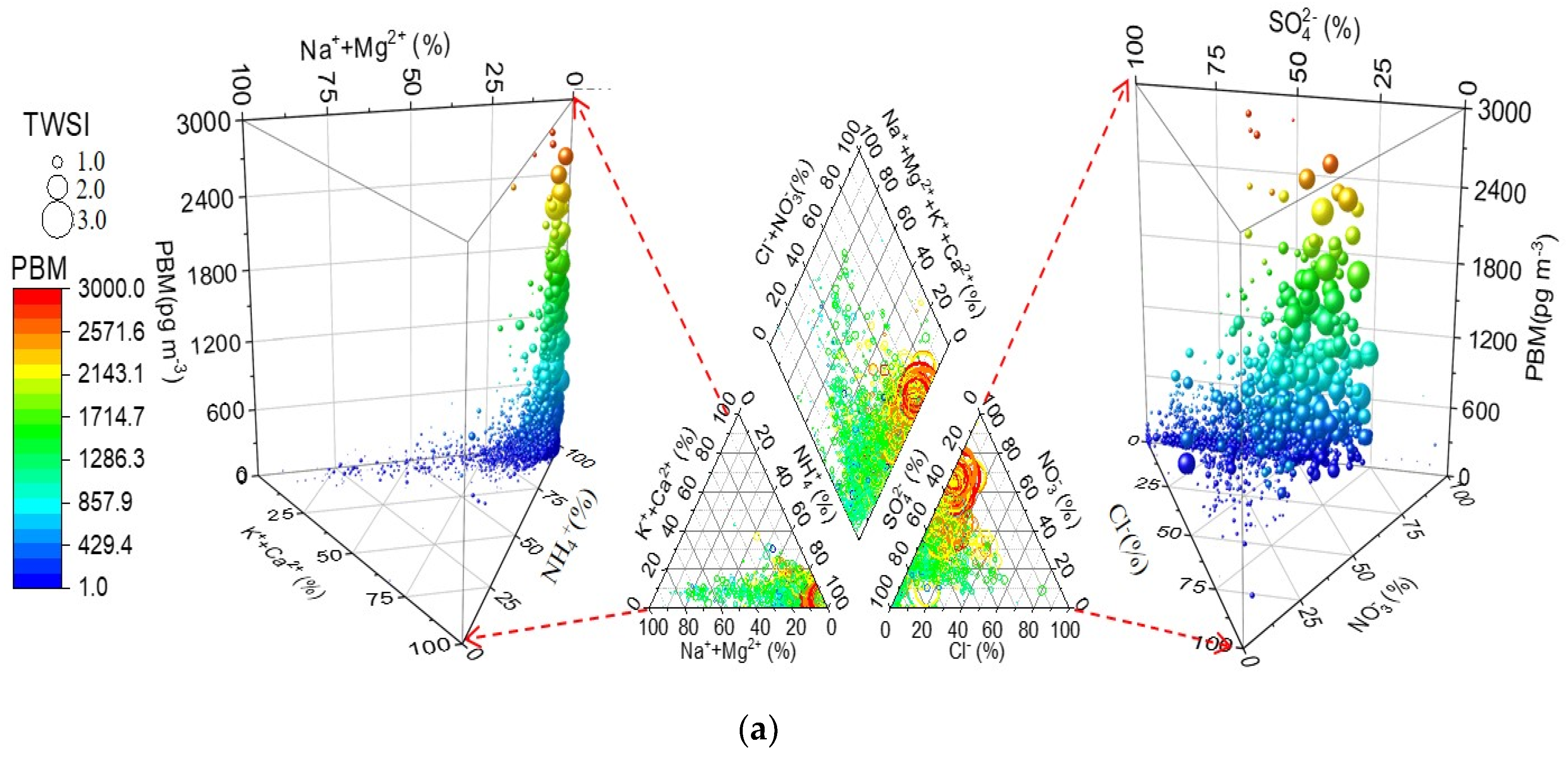
3.3. Piper Diagram Analysis

As shown in Figure 3, the rhombohedral panel and the right ternary panel in the Piper diagrams showed that the scatter points with high GEM and PBM concentrations gathered at the SO42− axis, and the corresponding points in the left ternary panel gradually converged at the right corner. Both GEM and PBM exhibited similar and regular trends in variations with the changes in the percentage values of cation and anion normality, i.e., the concentrations of GEM, PBM and TWSI normality generally increased with the increasing percentage values of NH4+ in cationic normality and those of NO3 in anionic normality, and increased with the decreasing percentage values of Na+ + Mg2+, Cl and SO42− normality. The peak values of GEM and PBM were observed when the percentage values of NH4+ and Na+ + Mg2+ in cationic normality were close to 100% and 0, respectively, and when those of NO3 and SO42− in anionic normality were close to 60% and 40%, respectively. Na+, Mg2+ and Cl are the primary components of sea salt, and were found to mainly originate from oceanic emissions. It was found that the contribution of oceanic emissions to GEM and PBM pollution was negligible. The near-exponential decreases in the GEM and PBM concentrations with the increasing percentage values of Na+ + Mg2+ in cationic normality indicated the quantifiable dilution effect of clean marine airmass coming from the East China Sea (Figure 2 and Figure 3). NH4+, NO3 and SO42− are mainly formed via the secondary reactions of atmospheric precursors (e.g., NH3, NOx and SO2), which are directly emitted from anthropogenic sources and closely associated with GEM and PBM emissions. In addition, both GEM and PBM concentrations exhibited positive correlations with the percentage values of NH4+ (r = 0.6, 0.35; p < 0.01) and NO3 (r = 0.41, 0.45; p < 0.01) normality, and negative correlations with the percentage values of SO42− normality (r = −0.38, −0.44; p < 0.01). This indicated the contribution of polluted air mass with increased NH4+ and NO3 concentrations to the aggravation of GEM and PBM pollution at the study site.
As for GOM, no close relationship between this mercury species and WSIIs was found using the Piper diagram (Figure S2). GOM is different from GEM and PBM in terms of physicochemical properties. It can be directly emitted from anthropogenic sources or formed indirectly from GEM via photochemical reactions. The oxidation of GEM to GOM by ozone- or marine-originating halogen radicals has been reported to occur in mid-latitude areas [53]. The concentration of GOM might be significantly changed during atmospheric transport. This might account for the poor relationship between GOM and WSIIs.

3.4. Pollution Episode Analysis

A typical pollution episode (lasting for 3 days) caused by coal combustion with significantly elevated GEM concentrations was observed from 21 October to 24 October 2017 (Figure 4). During the pollution period, the dominant wind at NUEORS was from the northwest, and carried a considerable amount of air pollutants from the industrial and urban areas of Ningbo. The 72 h backward trajectories (Figure S3) showed that the air masses gradually approached the Beilun coal-fired power plant from October 21 to October 22, and departed from 23 October to 24 October. The most distinctive feature of Figure S3b,d is that, as the perpendicular distance between the Beilun coal-fired power plant and the air masses decreases, the concentrations of GEM and PM2.5 increase. The hourly average GEM concentrations steadily increased from 14:00 of 21 October to 13:00 of 22 October, with a maximum of 4.1 ng m−3, and then decreased to the minimum of 1.7 ng m−3 at 04:00 on October 24. The concentrations of GEM, GOM and PBM during the pollution period were in the range of 2.0~4.1 ng m−3, 4.5~467.5 pg m−3 and 36.4~976.7 pg m−3, with average values of 2.8 ng m−3, 97.4 pg m−3 and 375.4 pg m−3, respectively. Before the pollution period, the average concentrations of GEM, GOM and PBM were 1.9 ng m−3, 25.9 pg m−3 and 79.5 pg m−3, respectively. The concentrations of these species were 1.9 ng m−3, 157.4 pg m−3 and 184.1 pg m−3, respectively, which were observed after the pollution period. During the pollution episode, PM2.5, WSIIs (including SO42−, NO3, NH4+, K+ and Cl), SO2 and NO2 generally exhibited synchronous variations with GEM and PBM, and positive correlations were observed between GEM and PM2.5, SO42−, NO3, NH4+, K+, Cl, SO2 and NO2 (r = 0.35–0.74, p-value < 0.01) (Table S2). As for PBM, it showed positive correlations with PM2.5, NO3, NH4+, K+, Cl, Ca2+, SO2 and NO2 (r = 0.36–0.67, p-value < 0.01). Compared to GEM, PBM exhibited no significant correlation with SO42−, but there was a weak correlation between PBM and Ca2+ during the pollution episode (r = 0.36, p-value < 0.01). In addition, PBM was strongly correlated with GEM (r = 0.65, p-value < 0.01). These results indicated that GEM and PBM might originate from the same sources, such as from fossil fuel or municipal waste combustion. During the pollution episode, GOM was only positively correlated with O3 (r = 0.31, p-value < 0.05). Ozone is generally one of the dominant oxidants for GEM. The gas–phase oxidation of GEM by O3 might be an important source for GOM formation. However, we failed to find significant correlations between GOM and GEM or PBM (r < 0.1) during the pollution episode. This suggested that the sources of GOM might be different from those of GEM and PBM in the study area. However, more field measurement campaigns are needed to further confirm this.

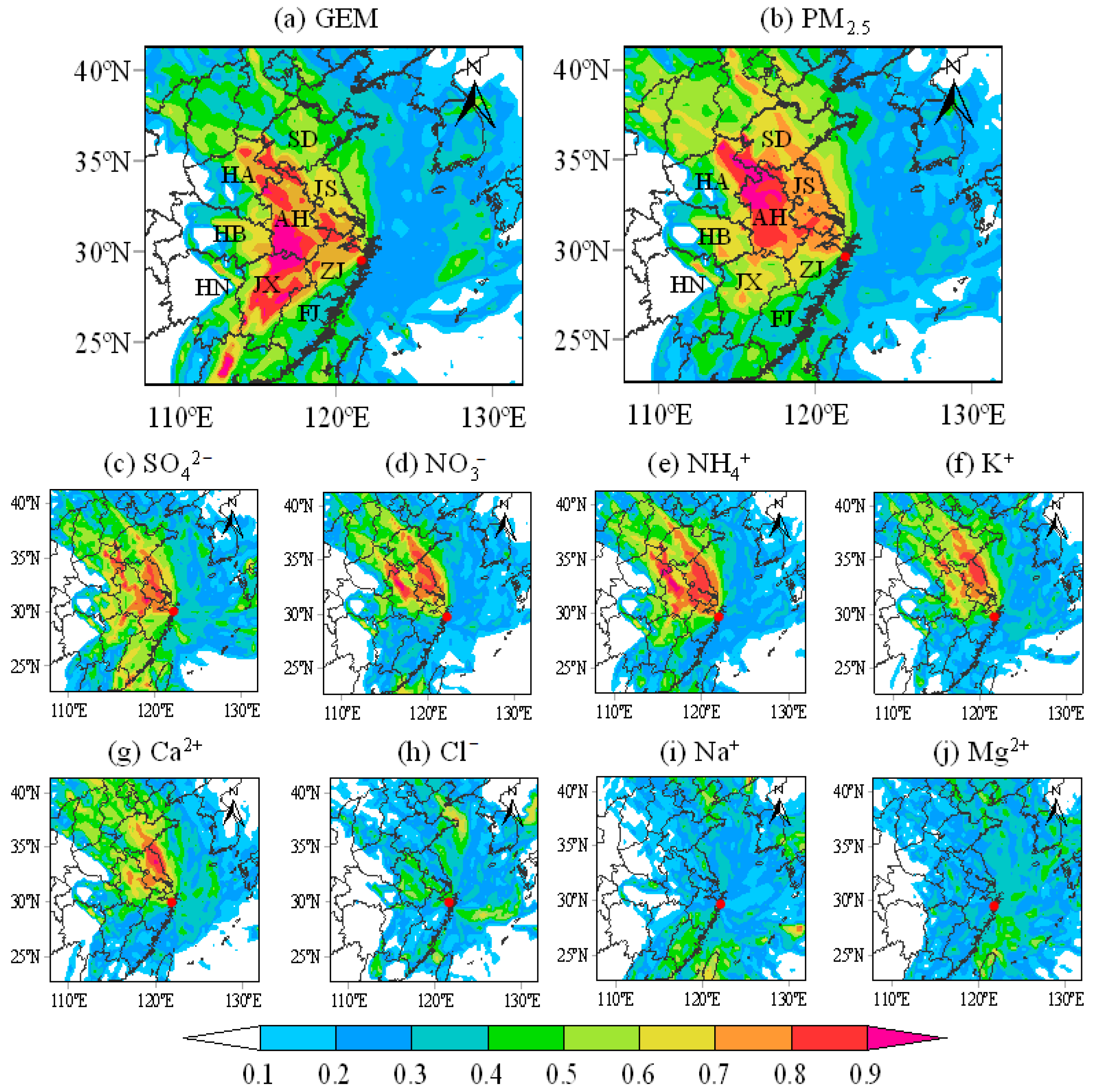
3.5. Potential Source Contribution Function Analysis (PSCF)

In this study, PSCF was used to identify and compare the potential source regions of GEM, PM2.5 and WSIIs at the study site (Figure 5). During the whole study period, the PSCF values for GEM at the neighboring provinces were very high, and it was found that the potential source regions of GEM (magenta area in Figure 5a) lie mainly in Anhui, Jiangxi, northern Zhejiang, and the border areas among eastern Anhui and southern Jiangsu. It can be found that the potential source regions of GEM were similar to those of PM2.5, SO42−, NO3, NH4+, K+ and Ca2+ (Figure 5b–g), which indicated that these species might originate from the same areas. These regions were mainly in the developed coastal provinces of eastern China (Shandong, Jiangsu, Zhejiang and Guangdong) and inland provinces of central China (Anhui, Henan and Jiangxi), with dense manufacturing industry (eastern China), developed non-ferrous metal smelting and coal production (middle area of China) [54]. These source regions are mainly located on the northwestern and western sides of the study site, and were found to potentially emit large amounts of GEM and PM2.5 into the atmosphere annually. Air masses passing over these regions could carry air pollutants to the study area, potentially playing an important role in enhancing the local atmospheric concentrations of these species. Therefore, the long-range transportation of GEM and PM2.5 from these regions is one of the main reasons for the GEM and PM2.5 pollution at the study site. This agrees well with previous studies [55,56]. As reported by Li et al. [57], there are heavily mercuric-polluted regions in the provinces (e.g., Guizhou) of western China. However, the influence of the long-range transport of air pollutants from western China on the level of atmospheric mercury at the study site is negligible compared to the contribution from central and eastern China. This is mainly due to a lack of polluted air masses passing over these areas and arriving at the study site. In addition, the PSCF values for GEM, PM2.5, SO42−, NO3, NH4+, K+ and Ca2+ of the air masses from the East China Sea were lower than those from other directions. This indicated that the dilution effect of clean marine air mass and the enhanced oxidation of GEM by the relatively high levels of O3 and halogens over the sea are important for GEM depletion in coastal areas [36,37].
In contrast, high PSCF values for Cl, Na+ and Mg2+ were generally observed in marine areas, including the Taiwan Strait, East China Sea and Bohai Sea (Figure 5h–j). This was expected because Cl, Na+ and Mg2+ are the dominant components of sea salt, and thus mainly originated from sea spray [45]. Notably, slightly elevated PSCF values (0.5~0.7) for Cl were observed in the northwest of the study site. This might be due to the anthropogenic emissions generated by coal combustion for heating. A previous study had also reported that fossil fuel burning is one of the major emission sources of Cl in the atmosphere [58]. This might account for the elevated PSCF values observed over the land area.

3.6. Empirical Algorithms for Mercury Species Simulations

According to the results of the correlation analysis (Table 2) in the previous section, we noted that the major conventional air pollutants with high correlations with GEM were PM2.5, NOx and CO, all of which exhibited good linear relationships with GEM. These three species are mainly emitted from anthropogenic sources, suggesting the significant contribution of land sources to atmospheric elemental mercury. In contrast, Na+ and Mg2+, which are mainly emitted from marine sources, exhibited a near-exponential relationship with GEM, based on the percentage values of their cationic normality (Figure 6). This indicated the significant dilution and cleaning effects of marine airmass on atmospheric mercury. Based on the above findings, we developed an empirical algorithm for GEM simulation in this section, considering the contributions of both terrestrial and oceanic sources. The algorithm is defined mathematically with the combination of multiple linear function and exponential function. The indicial form of the constructed algorithm is presented in Equation (2):
GEM = a × exp(b × [Na+ + Mg2+]) + c × PM2.5 + dCO + e × NOx + s
where [Na+ + Mg2+] represents the percentage values of Na+ + Mg2+ in cationic normality; a, b, c, d and e represent the coefficients of each variable; and s denotes the constant term.
Equation (2) was solved numerically using the iterative regressions based on the one-year monitoring data at the study site (from December 2016 to November 2017); the derived algorithms are presented in Equation (3):
GEM = 0.69146 × exp(−0.14914 × [Na+ + Mg2+]) + 0.02307 × PM2.5 + 0.61165 × CO + 0.00643 × NOx + 1.13632
Overall, an R2 value of 0.55 for the iterative regressions was considered to be acceptable (MAE: 0.39, MAPE: 16.47%, RMSE: 0.60). In addition, a set of data obtained from 28 February to 14 April 2018 was used to test our algorithm. The comparison between the measured and predicted GEM showed that the variation in GEM concentrations could be well predicted comprehensively by PM2.5, NOx, CO and the percentage value of Na+ + Mg2+ cationic normality (R2 = 0.79, p < 0.01) (Figure 7). It is evident that the predicted GEM concentrations sometimes deviate from the actual observed concentrations, either above or below. The reasons for these deviations are complex and could be attributed to sudden and significant changes in pollution sources or specific meteorological conditions. Also, it is worth noting that the applicability of the model is limited because the data used in the model are specific to a single site. Therefore, it is necessary to optimize and adjust the model appropriately when dealing with other areas that have significant differences in pollution sources.

4. Conclusions

In this study, the pollution characteristics of atmospheric mercury species (GEM, GOM and PBM) and their relationships with water-soluble inorganic ions were analyzed. The GEM concentrations (2.4 ng m−3) at the study site in Ningbo were generally higher than those of the remote background and rural sites in the Northern Hemisphere; meanwhile, they were lower than those of most urban and suburban areas in Asia. The concentrations of GOM (99.3 pg m−3) and PBM (286.5 pg m−3) were higher than those reported for most other sites worldwide due to direct industrial emissions and secondary production via photochemical reactions in the coastal regions of East China. Generally, synchronous variations were observed for the monthly average concentrations of GEM, PBM, TWSI and PM2.5, which indicated that the speciated mercury and fine particulate in the study region had similar anthropogenic sources. GEM and PBM roughly increased with the increasing percentage values of NH4+ normality, and decreased exponentially with the increasing sum of the percentage values of Na+ and Mg2+ normality; this indicated the contribution of an ammonium-salt-abundant airmass to local mercury pollution and the dilution effect of clean marine airmass from the East China Sea to atmospheric mercury. The potential source regions of GEM were similar to those of PM2.5, SO42−, NO3, NH4+, K+ and Ca2+. The temporal trend observed in GEM was predicted well using an empirical algorithm. The interrelated pollution characteristics of the atmospheric speciated mercury and water-soluble inorganic ions derived in this study could provide useful insights into the transport and transformation mechanism of mercury in the coastal area of east China. The newly developed model could serve as an auxiliary model for available mercury prediction methods, as well as a potential substitute for GEM measurement.

Supplementary Materials

The following supporting information can be downloaded at: https://www.mdpi.com/article/10.3390/atmos14111594/s1, Figure S1: Schematic of the Piper diagram; Figure S2: The relationship between GOM and WSIIs; Figure S3: 72-h backward trajectories during the pollution episode; Table S1: Summary of GEM, GOM, PBM, PM2.5 and WSIIs concentrations; Table S2: The Spearman correlation of speciated mercury with WSIIs and conventional pollutants during the pollution episode from 21 October to 24 October 2017.

Author Contributions

Conceptualization, H.X. and H.Y.; methodology, H.X.; software, Z.H.; validation, J.L., D.L. and H.Y.; formal analysis, H.Y.; investigation, L.T.; resources, L.X.; data curation, H.Y.; writing—original draft preparation, H.Y.; writing—review and editing, L.T.; visualization, D.L.; supervision, H.X.; project administration, L.T.; funding acquisition, H.X. All authors have read and agreed to the published version of the manuscript.

Funding

This research was funded by National Natural Science Foundation of China (Grant No. 21976171); Strategic Pilot Project of Chinese Academy of Sciences (Grant No. XDA23020000); Guangxi Key Research and Development Program (Grant No. GuikeAB21220063); Ningbo Natural Science Foundation of China (Grant No. 2023J059); Chaozhou Science and Technology Program (Grant No. 2018GY03).

Institutional Review Board Statement

Not applicable.

Informed Consent Statement

Not applicable.

Data Availability Statement

The data presented in this study are available on request from the corresponding author. The data are not publicly available due to restrictions and privacy.

Conflicts of Interest

The authors declare no conflict of interest.

References

  1. Huo, H.; Zhang, Q.; Guan, D.B.; Su, X.; Zhao, H.Y.; He, K.B. Examining Air Pollution in China Using Production- And Consumption-Based Emissions Accounting Approaches. Environ. Sci. Technol. 2014, 48, 14139–14147. [Google Scholar] [CrossRef]
  2. Carocci, A.; Rovito, N.; Sinicropi, M.S.; Genchi, G. Mercury Toxicity and Neurodegenerative Effects. Rev. Environ. Contam. Toxicol. 2014, 229, 1–18. [Google Scholar] [PubMed]
  3. Mao, H.; Talbot, R.; Hegarty, J.; Koermer, J. Speciated Mercury at Marine, Coastal, and Inland Sites in New England–Part 2: Relationships with Atmospheric Physical Parameters. Atmos. Chem. Phys. 2012, 12, 4181–4206. [Google Scholar] [CrossRef]
  4. Howard, D.; Nelson, P.F.; Edwards, G.C.; Morrison, A.L.; Fisher, J.A.; Ward, J.; Harnwell, J.; van der Schoot, M.; Atkinson, B.; Chambers, S.D.; et al. Atmospheric Mercury in the Southern Hemisphere Tropics: Seasonal and Diurnal Variations and Influence of Inter-Hemispheric Transport. Atmos. Chem. Phys. 2017, 17, 11623–11636. [Google Scholar] [CrossRef]
  5. Selin, N.E.; Jacob, D.J.; Park, R.J.; Yantosca, R.M.; Strode, S.; Jaegle, L.; Jaffe, D. Chemical Cycling and Deposition of Atmospheric Mercury: Global Constraints from Observations. J. Geophys. Res. Atmos. 2007, 112, D02308. [Google Scholar] [CrossRef]
  6. Bergan, T.; Rodhe, H. Oxidation of Elemental Mercury in the Atmosphere; Constraints Imposed by Global Scale Modelling. J. Atmos. Chem. 2001, 40, 191–212. [Google Scholar] [CrossRef]
  7. Duan, L.; Wang, X.H.; Wang, D.F.; Duan, Y.S.; Cheng, N.; Xiu, G.L. Atmospheric Mercury Speciation in Shanghai, China. Sci. Total Environ. 2017, 578, 460–468. [Google Scholar] [CrossRef]
  8. Pongprueksa, P.; Lin, C.J.; Lindberg, S.E.; Jang, C.; Braverman, T.; Bullock, O.R.; Ho, T.C.; Chu, H.W. Scientific Uncertainties in Atmospheric Mercury Models III: Boundary and Initial Conditions, Model Grid Resolution, and Hg(II) Reduction Mechanism. Atmos. Environ. 2008, 42, 1828–1845. [Google Scholar] [CrossRef]
  9. Si, L.; Ariya, P.A. Reduction of Oxidized Mercury Species by Dicarboxylic Acids (C(2)–C(4)): Kinetic and Product Studies. Environ. Sci. Technol. 2008, 42, 5150–5155. [Google Scholar] [CrossRef]
  10. Rutter, A.P.; Schauer, J.J. The Impact of Aerosol Composition on the Particle to Gas Partitioning of Reactive Mercury. Environ. Sci. Technol. 2007, 41, 3934–3939. [Google Scholar] [CrossRef]
  11. Subir, M.; Ariya, P.A.; Dastoor, A.P. A Review of the Sources of Uncertainties in Atmospheric Mercury Modeling II. Mercury Surface and Heterogeneous Chemistry—A Missing Link. Atmos. Environ. 2012, 46, 1–10. [Google Scholar] [CrossRef]
  12. Baya, A.P.; Van Heyst, B. Assessing the Trends and Effects of Environmental Parameters on the Behaviour of Mercury in the Lower Atmosphere over Cropped Land Over Four Seasons. Atmos. Chem. Phys. 2010, 10, 8617–8628. [Google Scholar] [CrossRef]
  13. Brooks, S.; Moore, C.; Lew, D.; Lefer, B.; Huey, G.; Tanner, D. Temperature and Sunlight Controls of Mercury Oxidation and Deposition Atop the Greenland Ice Sheet. Atmos. Chem. Phys. 2011, 11, 8295–8306. [Google Scholar] [CrossRef]
  14. Chand, D.; Jaffe, D.; Prestbo, E.; Swartzendruber, P.C.; Hafner, W.; Weiss-Penzias, P.; Kato, S.; Takami, A.; Hatakeyama, S.; Kajii, Y.Z. Reactive and Particulate Mercury in the Asian Marine Boundary Layer. Atmos. Environ. 2008, 42, 7988–7996. [Google Scholar] [CrossRef]
  15. Liu, B.; Keeler, G.J.; Dvonch, J.T.; Barres, J.A.; Lynam, M.M.; Marsik, F.J.; Morgan, J.T. Urban-Rural Differences in Atmospheric Mercury Speciation. Atmos. Environ. 2010, 44, 2013–2023. [Google Scholar] [CrossRef]
  16. Sheu, G.R.; Lin, N.H.; Wang, J.L.; Lee, C.T.; Yang, C.F.O.; Wang, S.H. Temporal Distribution and Potential Sources of Atmospheric Mercury Measured at A High-Elevation Background Station in Taiwan. Atmos. Environ. 2010, 44, 2393–2400. [Google Scholar] [CrossRef]
  17. Steen, A.O.; Berg, T.; Dastoor, A.P.; Durnford, D.A.; Engelsen, O.; Hole, L.R.; Pfaffhuber, K.A. Natural and Anthropogenic Atmospheric Mercury in the European Arctic: A Fractionation Study. Atmos. Chem. Phys. 2011, 11, 6273–6284. [Google Scholar] [CrossRef]
  18. Fu, X.W.; Feng, X.B.; Qiu, G.L.; Shang, L.H.; Zhang, H. Speciated Atmospheric Mercury and its Potential Source in Guiyang, China. Atmos. Environ. 2011, 45, 4205–4212. [Google Scholar] [CrossRef]
  19. Kim, S.H.; Han, Y.J.; Holsen, T.M.; Yi, S.M. Characteristics of Atmospheric Speciated Mercury Concentrations (TGM, Hg(II) and Hg(P)) in Seoul, Korea. Atmos. Environ. 2009, 43, 3267–3274. [Google Scholar] [CrossRef]
  20. Xu, L.L.; Chen, J.S.; Yang, L.M.; Niu, Z.C.; Tong, L.; Yin, L.Q.; Chen, Y.T. Characteristics and Sources of Atmospheric Mercury Speciation in a Coastal City, Xiamen, China. Chemosphere 2015, 119, 530–539. [Google Scholar] [CrossRef]
  21. Liang, S.; Wang, Y.F.; Cinnirella, S.; Pirrone, N. Atmospheric Mercury Footprints of Nations. Environ. Sci. Technol. 2015, 49, 3566–3574. [Google Scholar] [CrossRef] [PubMed]
  22. Lan, X.; Talbot, R.; Laine, P.; Torres, A.; Lefer, B.; Flynn, J. Atmospheric Mercury in the Barnett Shale Area, Texas: Implications for Emissions from Oil and Gas Processing. Environ. Sci. Technol. 2015, 49, 10692–10700. [Google Scholar] [CrossRef] [PubMed]
  23. Lyman, S.N.; Gustin, M.S. Determinants of Atmospheric Mercury Concentrations in Reno, Nevada, USA. Sci. Total Environ. 2009, 408, 431–438. [Google Scholar] [CrossRef] [PubMed]
  24. Radke, L.F.; Friedli, H.R.; Heikes, B.G. Atmospheric Mercury over the NE Pacific During Spring 2002: Gradients, Residence Time, Upper Troposphere Lower Stratosphere Loss, and Long-Range Transport. J. Geophys. Res. Atmos. 2007, 112, D19305. [Google Scholar] [CrossRef]
  25. Nie, X.; Mao, H.; Li, P.; Li, T.; Zhou, J.; Wu, Y.; Yang, M.; Zhen, J.; Wang, X.; Wang, Y. Total Gaseous Mercury in A Coastal City (Qingdao, China): Influence of Sea-Land Breeze and Regional Transport. Atmos. Environ. 2020, 235, 117633. [Google Scholar] [CrossRef]
  26. Yi, H.; Tong, L.; Lin, J.; Cai, Q. Temporal Variation and Long–Range Transport of Gaseous Elemental Mercury (GEM) over A Coastal Site of East China. Atmos. Res. 2020, 233, 123–133. [Google Scholar] [CrossRef]
  27. Dastoor, A.; Ryzhkov, A.; Dumford, D.; Lehnherr, I.; Steffen, A.; Morrison, H. Atmospheric Mercury in the Canadian Arctic. Part II: Insight from Modeling. Sci. Total Environ. 2015, 509, 16–27. [Google Scholar] [CrossRef]
  28. Tang, Y.; Wang, S.; Wu, Q.; Liu, K.; Wang, L.; Li, S.; Gao, W.; Zhang, L.; Zheng, H.; Li, Z.; et al. Recent Decrease Trend of Atmospheric Mercury Concentrations in East China: The Influence of Anthropogenic Emissions. Atmos. Chem. Phys. 2018, 18, 8279–8291. [Google Scholar] [CrossRef]
  29. Fu, X.; Wang, S.; Zhao, B.; Xing, J.; Cheng, Z.; Liu, H.; Hao, J. Emission Inventory of Primary Pollutants and Chemical Speciation in 2010 for the Yangtze River Delta Region, China. Atmos. Environ. 2013, 70, 39–50. [Google Scholar] [CrossRef]
  30. Cheng, I.; Zhang, L. Uncertainty Assessment of Gaseous Oxidized Mercury Measurements Collected by Atmospheric Mercury Network. Environ. Sci. Technol. 2017, 51, 855–862. [Google Scholar] [CrossRef]
  31. Rodelas, R.R.; Perdrix, E.; Herbin, B.; Riffault, V. Characterization and Variability of Inorganic Aerosols and Their Gaseous Precursors at A Suburban Site in Northern France over One Year (2015–2016). Atmos. Environ. 2019, 200, 142–157. [Google Scholar] [CrossRef]
  32. Rumsey, I.C.; Cowen, K.A.; Walker, J.T.; Kelly, T.J.; Hanft, E.A.; Mishoe, K.; Rogers, C.; Proost, R.; Beachley, G.M.; Lear, G.; et al. An Assessment of the Performance of the Monitor for Aerosols and Gases in Ambient Air (MARGA): A Semi-Continuous Method for Soluble Compounds. Atmos. Chem. Phys. 2014, 14, 5639–5658. [Google Scholar] [CrossRef]
  33. Cai, Q.L.; Dai, X.R.; Li, J.R.; Tong, L.; Hui, Y.; Cao, M.Y.; Li, M.; Xiao, H. The Characteristics and Mixing States of PM2.5 during A Winter Dust Storm in Ningbo of the Yangtze River Delta, China. Sci. Total Environ. 2020, 709, 136136. [Google Scholar] [CrossRef] [PubMed]
  34. Wang, Y.Q.; Zhang, X.Y.; Draxler, R.R. TrajStat: GIS-based Software that Uses Various Trajectory Statistical Analysis Methods to Identify Potential Sources from Long-Term Air Pollution Measurement Data. Environ. Model. Softw. 2009, 24, 938–939. [Google Scholar] [CrossRef]
  35. Huang, J.Y.; Liu, C.K.; Huang, C.S.; Fang, G.C. Atmospheric Mercury Pollution at An Urban Site in Central Taiwan: Mercury Emission Sources at Ground Level. Chemosphere 2012, 87, 579–585. [Google Scholar] [CrossRef]
  36. Holmes, C.D.; Jacob, D.J.; Mason, R.P.; Jaffe, D.A. Sources and Deposition of Reactive Gaseous Mercury in the Marine Atmosphere. Atmos. Environ. 2009, 43, 2278–2285. [Google Scholar] [CrossRef]
  37. Tong, L.; Zhang, H.L.; Yu, J.; He, M.M.; Xu, N.B.; Zhang, J.J.; Qian, F.Z.; Feng, J.Y.; Xiao, H. Characteristics of Surface Ozone and Nitrogen Oxides at Urban, Suburban and Rural Sites in Ningbo, China. Atmos. Res. 2017, 187, 57–68. [Google Scholar] [CrossRef]
  38. Nair, U.S.; Wu, Y.L.; Walters, J.; Jansen, J.; Edgerton, E.S. Diurnal and Seasonal Variation of Mercury Species at Coastal-Suburban, Urban, and Rural Sites in the Southeastern United States. Atmos. Environ. 2012, 47, 499–508. [Google Scholar] [CrossRef]
  39. Choi, H.D.; Huang, J.Y.; Mondal, S.; Holsen, T.M. Variation in Concentrations of Three Mercury (Hg) Forms at A Rural and A Suburban Site in New York State. Sci. Total Environ. 2013, 448, 96–106. [Google Scholar] [CrossRef]
  40. Huang, J.Y.; Hopke, P.K.; Choi, H.D.; Laing, J.R.; Cui, H.L.E.; Zananski, T.J.; Chandrasekaran, S.R.; Rattigan, O.V.; Holsen, T.M. Mercury (Hg) Emissions from Domestic Biomass Combustion for Space Heating. Chemosphere 2011, 84, 1694–1699. [Google Scholar] [CrossRef]
  41. Matsunaga, S.; Mochida, M.; Kawamura, K. Growth of Organic Aerosols by Biogenic Semi-Volatile Carbonyls in the Forestal Atmosphere. Atmos. Environ. 2003, 37, 2045–2050. [Google Scholar] [CrossRef]
  42. Rutter, A.P.; Schauer, J.J. The Effect of Temperature on the Gas-Particle Partitioning of Reactive Mercury in Atmospheric Aerosols. Atmos. Environ. 2007, 41, 8647–8657. [Google Scholar] [CrossRef]
  43. Steffen, A.; Douglas, T.; Amyot, M.; Ariya, P.; Aspmo, K.; Berg, T.; Bottenheim, J.; Brooks, S.; Cobbett, F.; Dastoor, A.; et al. A Synthesis of Atmospheric Mercury Depletion Event Chemistry in the Atmosphere and Snow. Atmos. Chem. Phys. 2008, 8, 1445–1482. [Google Scholar] [CrossRef]
  44. Wang, Y.G.; Huang, J.Y.; Hopke, P.K.; Rattigan, O.V.; Chalupa, D.C.; Utell, M.J.; Holsen, T.M. Effect of the Shutdown of a Large Coal-Fired Power Plant on Ambient Mercury Species. Chemosphere 2013, 92, 360–367. [Google Scholar] [CrossRef]
  45. Zhang, J.J.; Tong, L.; Huang, Z.W.; Zhang, H.L.; He, M.M.; Dai, X.R.; Zheng, J.; Xiao, H. Seasonal Variation and Size Distributions of Water-Soluble Inorganic Ions and Carbonaceous Aerosols at A Coastal Site in Ningbo, China. Sci. Total Environ. 2018, 639, 793–803. [Google Scholar] [CrossRef]
  46. Berg, T.; Fjeld, E.; Steinnes, E. Atmospheric Mercury in Norway: Contributions from Different Sources. Sci. Total Environ. 2006, 368, 3–9. [Google Scholar] [CrossRef]
  47. Castro, P.J.; Kellö, V.; Cernušák, I.; Dibble, T.S. Together, not Separately, OH and O3 Oxidize Hg(0) to Hg(II) in the Atmosphere. J. Phys. Chem. A 2022, 126, 8266–8279. [Google Scholar] [CrossRef]
  48. Lee, S.H.; Lee, J.I.; Han, Y.J.; Kim, P.R. Factors Influencing Concentrations of Atmospheric Speciated Mercury Measured at the Farthest Island West of South Korea. Atmos. Environ. 2019, 213, 239–249. [Google Scholar]
  49. Chen, X.J.; Balasubramanian, R.; Zhu, Q.Y.; Behera, S.N.; Bo, D.D.; Huang, X.; Xie, H.Y.; Cheng, J.P. Characteristics of Atmospheric Particulate Mercury in Size-Fractionated Particles during Haze Days in Shanghai. Atmos. Environ. 2016, 131, 400–408. [Google Scholar] [CrossRef]
  50. Lin, C.J.; Pehkonen, S.O. The Chemistry of Atmospheric Mercury: A Review. Atmos. Environ. 1999, 33, 2067–2079. [Google Scholar] [CrossRef]
  51. Ariya, P.A.; Amyot, M.; Dastoor, A.; Deeds, D.; Feinberg, A.; Kos, G.; Poulain, A.; Ryjkov, A.; Semeniuk, K.; Subir, M.; et al. Mercury Physicochemical and Biogeochemical Transformation in the Atmosphere and at Atmospheric Interfaces: A Review and Future Directions. Chem. Rev. 2015, 115, 3760–3802. [Google Scholar] [CrossRef]
  52. Deshmukh, D.K.; Deb, M.K.; Verma, D.; Nirmalkar, J. Seasonal Air Quality Profile of Size-Segregated Aerosols in the Ambient Air of A Central Indian Region. Bull. Environ. Contam. Toxicol. 2013, 91, 704–710. [Google Scholar] [CrossRef] [PubMed]
  53. Obrist, D.; Tas, E.; Peleg, M.; Matveev, V.; Fain, X.; Asaf, D.; Luria, M. Bromine-Induced Oxidation of Mercury in the Mid-Latitude Atmosphere. Nat. Geosci. 2011, 4, 22–26. [Google Scholar] [CrossRef]
  54. Ye, X.J.; Hu, D.; Wang, H.H.; Chen, L.; Xie, H.; Zhang, W.; Deng, C.Y.; Wang, X.J. Atmospheric Mercury Emissions from China’s Primary Nonferrous Metal (Zn, Pb and Cu) Smelting during 1949–2010. Atmos. Environ. 2015, 103, 331–338. [Google Scholar] [CrossRef]
  55. Schneider, L.; Mariani, M.; Saunders, K.M.; Maher, W.A.; Harrison, J.J.; Fletcher, M.S.; Zawadzki, A.; Heijnis, H.; Haberle, S.G. How Significant is Atmospheric Metal Contamination from Mining Activity Adjacent to the Tasmanian Wilderness World Heritage Area? A Spatial Analysis of Metal Concentrations Using Air Trajectories Models. Sci. Total Environ. 2019, 656, 250–260. [Google Scholar] [CrossRef] [PubMed]
  56. Sprovieri, F.; Pirrone, N.; Landis, M.S.; Stevens, R.K. Atmospheric Mercury Behavior at Different Altitudes at Ny Alesund During Spring 2003. Atmos. Environ. 2005, 39, 7646–7656. [Google Scholar] [CrossRef]
  57. Li, P.; Feng, X.B.; Qiu, G.L.; Shang, L.H.; Wang, S.F.; Meng, B. Atmospheric Mercury Emission from Artisanal Mercury Mining in Guizhou Province, Southwestern China. Atmos. Environ. 2009, 43, 2247–2251. [Google Scholar] [CrossRef]
  58. Liu, Z.R.; Xie, Y.Z.; Hu, B.; Wen, T.X.; Xin, J.Y.; Li, X.R.; Wang, Y.S. Size-Resolved Aerosol Water-Soluble Ions during the Summer and Winter Seasons in Beijing: Formation Mechanisms of Secondary Inorganic Aerosols. Chemosphere 2017, 183, 119–131. [Google Scholar] [CrossRef] [PubMed]
Figure 1. Location of the study site and the online monitoring instruments employed in this study. The base map of Chinese provincial boundaries was obtained from the Resource and Environment Science and Data Center: https://www.resdc.cn (accessed on 20 August 2023). The satellite image was obtained from Esri, Maxar, Earthstar Geographics, and the GIS User Community.
Atmosphere 14 01594 g001
Figure 2. Monthly variations in (a) GEM, (b) GOM, (c) PBM, (d) PM2.5 and (e) water-soluble inorganic ions during the sampling period at the study site.
Atmosphere 14 01594 g002
Figure 3. The relationships between atmospheric speciated mercury and WSIIs ((a) GEM, (b) PBM, the size of the circles represents the equivalent concentration of TWSI).
Atmosphere 14 01594 g003aAtmosphere 14 01594 g003b
Figure 4. The variations in the hourly average concentrations of speciated mercury, WSIIs and conventional pollutants during the pollution episode from 21 October to 24 October 2017. The colors for each variable match those on the axis label.
Atmosphere 14 01594 g004
Figure 5. The smoothed PSCF maps (at 500 m altitude) for (a) GEM, (b) PM2.5 and WSIIs ((c) SO42−, (d) NO3, (e) NH4+, (f) K+, (g) Ca2+, (h) Cl, (i) Na+ and (j) Mg2+) at the study site (red circle) (AH: Anhui province, FJ: Fujian province, GD: Guangdong province, HA: Henan province, HB: Hubei province, HN: Hunan province, JS: Jiangsu province, JX: Jiangxi province, ZJ: Zhejiang province).
Atmosphere 14 01594 g005
Figure 6. The exponential fitting between GEM and the percentage values of Na+ + Mg2+ cationic normality.
Atmosphere 14 01594 g006
Figure 7. The time-series of measured and predicted GEM concentrations from 28 February to 14 April 2018.
Atmosphere 14 01594 g007
Table 1. Concentrations of ambient mercury species and PM2.5 measured in this and previous studies.
LocationClassificationGEM (ng m−3)GOM (pg m−3)PBM (pg m−3)PM2.5 (μg m−3)Time PeriodReference
Ningbo, ChinaCoastal2.499.3286.525.1December 2016~November 2017This study
Shanghai, ChinaSuburban4.221.1197.8-2014[7]
Xiamen, ChinaSuburban3.561.1174.4-March 2012~March 2013[20]
Guiyang, ChinaUrban/Mining area9.735.7368-August 2009~December 2009[18]
Lulin, TaiwanBackground and high elevation1.712.12.3-April 2006~December 2007[16]
Taichuang, TaiwanUrban/Industrial6.1332.071.1-March 2010~February 2011[35]
Seoul, KoreaUrban3.227.223.937.7February 2005~February 2006[19]
Cape Hedo, JapanRemote2.04.53.0-March 2004~May 2004[14]
Spitsbergen, European Arctic Rural1.68.08.0-April 2007~December 2008[17]
Summit, GreenlandRemote1.141.637.2 May 2007~June 2007[13]
Nova Scotia, CanadaRural/Coastal1.215.116.4-November 2006~August 2007[12]
Detroit, USAUrban/Industrial2.515.518.1-2004[15]
Dexter, USARural1.63.86.1-2004[15]
Atlanta, USARural1.48.64.4-2005~2008[38]
New York, USASuburban1.611.05.3-December 2007~December 2009[39]
Average of above cities2.92 ± 2.3146.44 ± 83.0581.5 ± 118.0731.4 ± 8.91
Note: the data in the table represent average values.
Table 2. Correlation analyses between speciated mercury and conventional air pollutants, meteorological variables and WSIIs.
GEMGOMPBMTGMKpPBM/TGM
SO20.26 **0.18 **0.46 **0.41 **-0.39 **
NO0.25 **-0.15 **0.21 **--
NO20.53 **-0.49 **0.55 **-0.36 **
NOx0.53 **-0.48 **0.55 **-0.36 **
CO0.53 **-0.32 **0.53 **-0.17 **
O3−0.20 **0.10 **−0.17 **−0.14 **−0.17 **-
PM100.49 **-0.48 **0.55 **-0.40 **
PM2.50.66 **0.11 **0.54 *0.69 **-0.42 **
Cl0.29 **-0.36 **0.40 **0.16 **0.36 **
NO30.60 **-0.49 **0.63 **0.13 **0.42 **
SO42−0.51 **-0.40 **0.58 **-0.42 **
Na+−0.16 **-−0.12 **−0.12 **-0.19 **
NH4+0.66 **-0.51 **0.70 **-0.46 **
K+0.51 **0.14 **0.56 **0.53 **0.15 **0.56 **
Mg2+−0.19 **--−0.14 **--
Ca2+0.25 **--0.36 **0.16 **0.44 **
TWSI0.62 **-0.66 **0.66 **-0.47 **
T−0.15 **−0.19 **−0.43 **−0.27 **-−0.44 **
RH-−0.16 **−0.24 **--−0.29 **
Note: *: p < 0.05; **: p < 0.01; -: r < 0.1 or p > 0.05.
Disclaimer/Publisher’s Note: The statements, opinions and data contained in all publications are solely those of the individual author(s) and contributor(s) and not of MDPI and/or the editor(s). MDPI and/or the editor(s) disclaim responsibility for any injury to people or property resulting from any ideas, methods, instructions or products referred to in the content.

