

The Heat Budget of the Tropical Pacific Mixed Layer during Two Types of El Niño Based on Reanalysis and Global Climate Model Data

Abstract
:1. Introduction
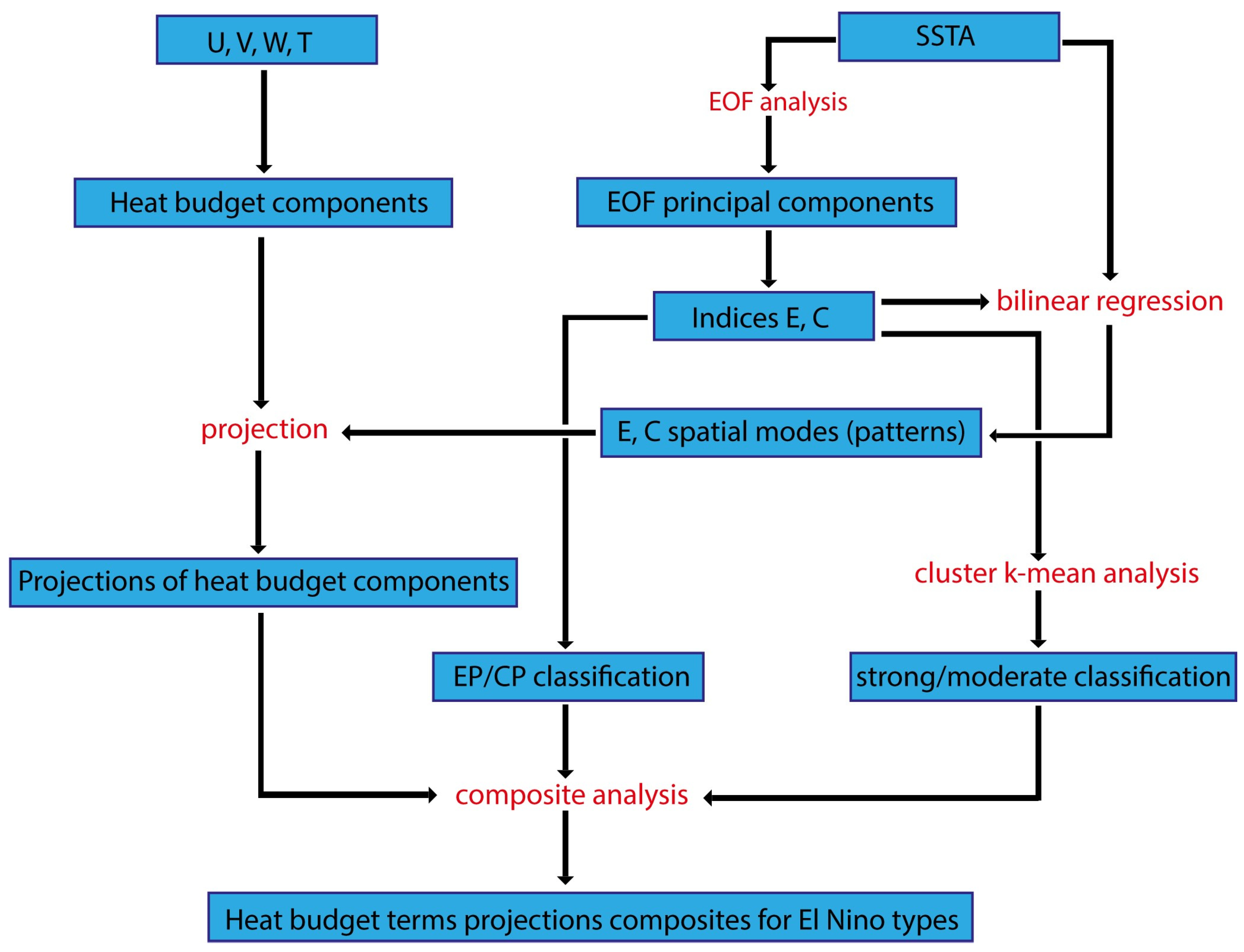
2. Materials and Methods
2.1. Data
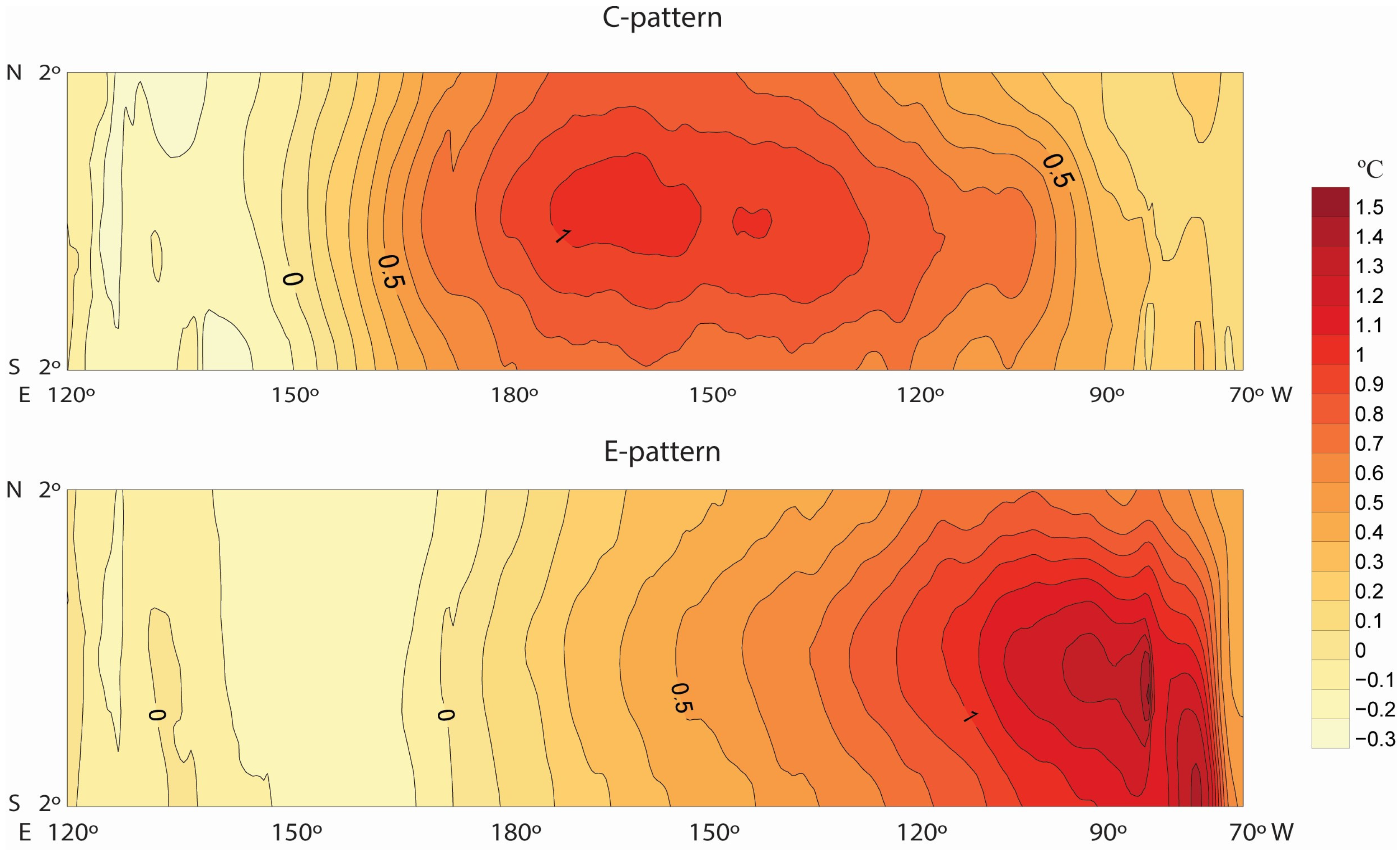
2.2. El Niño Definition
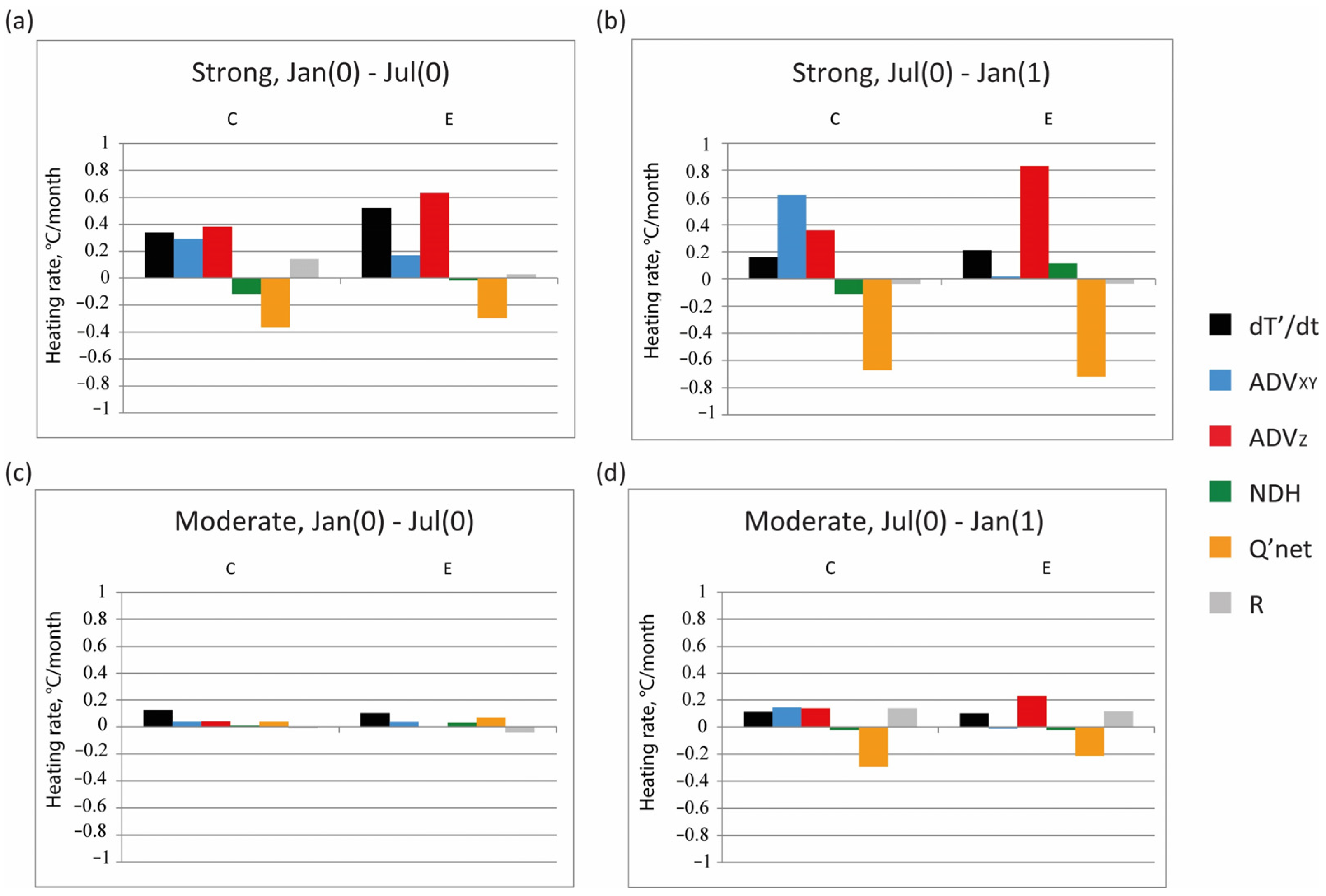
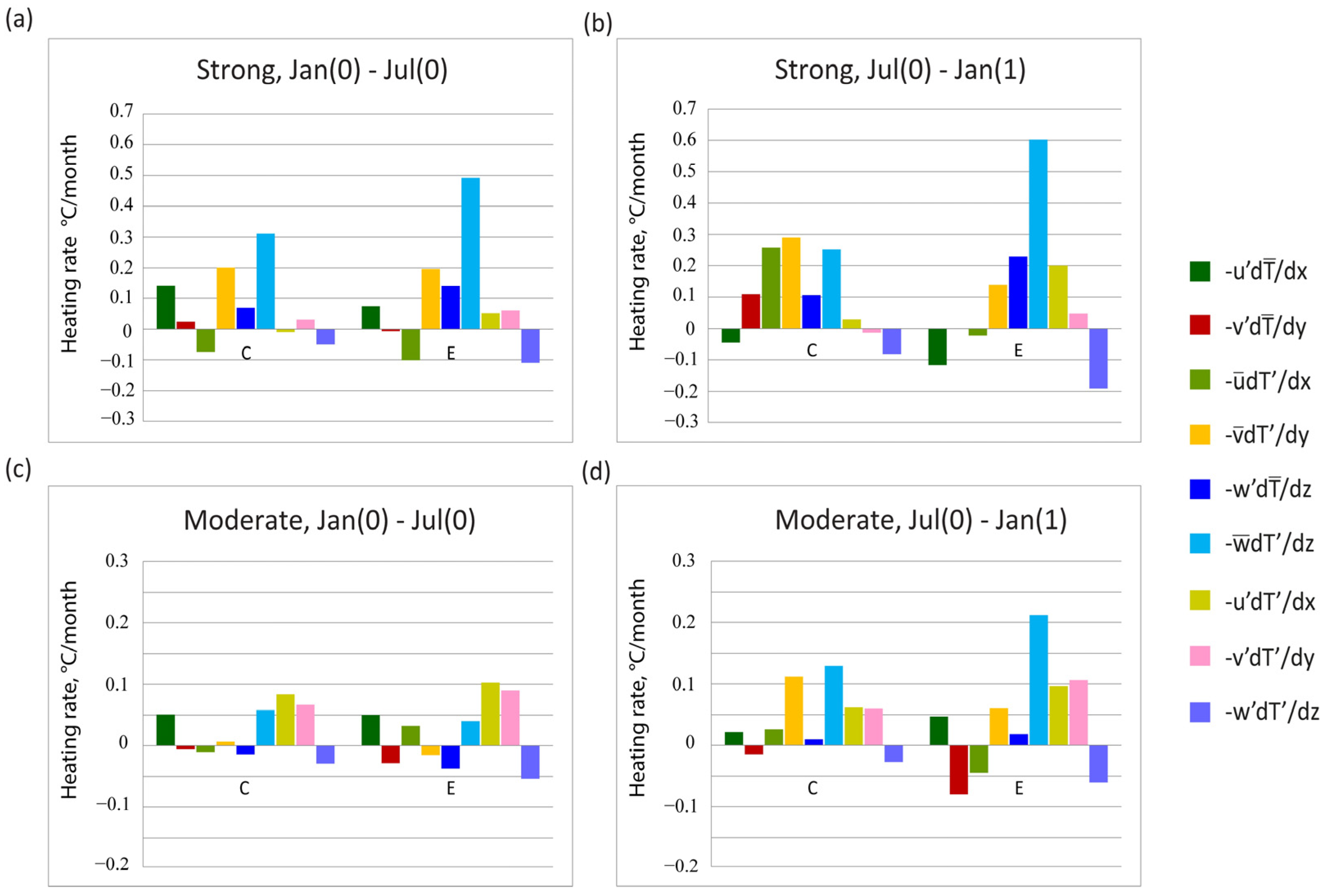
2.3. The Heat Budget of the Ocean Upper Mixed Layer
3. Results and Discussion
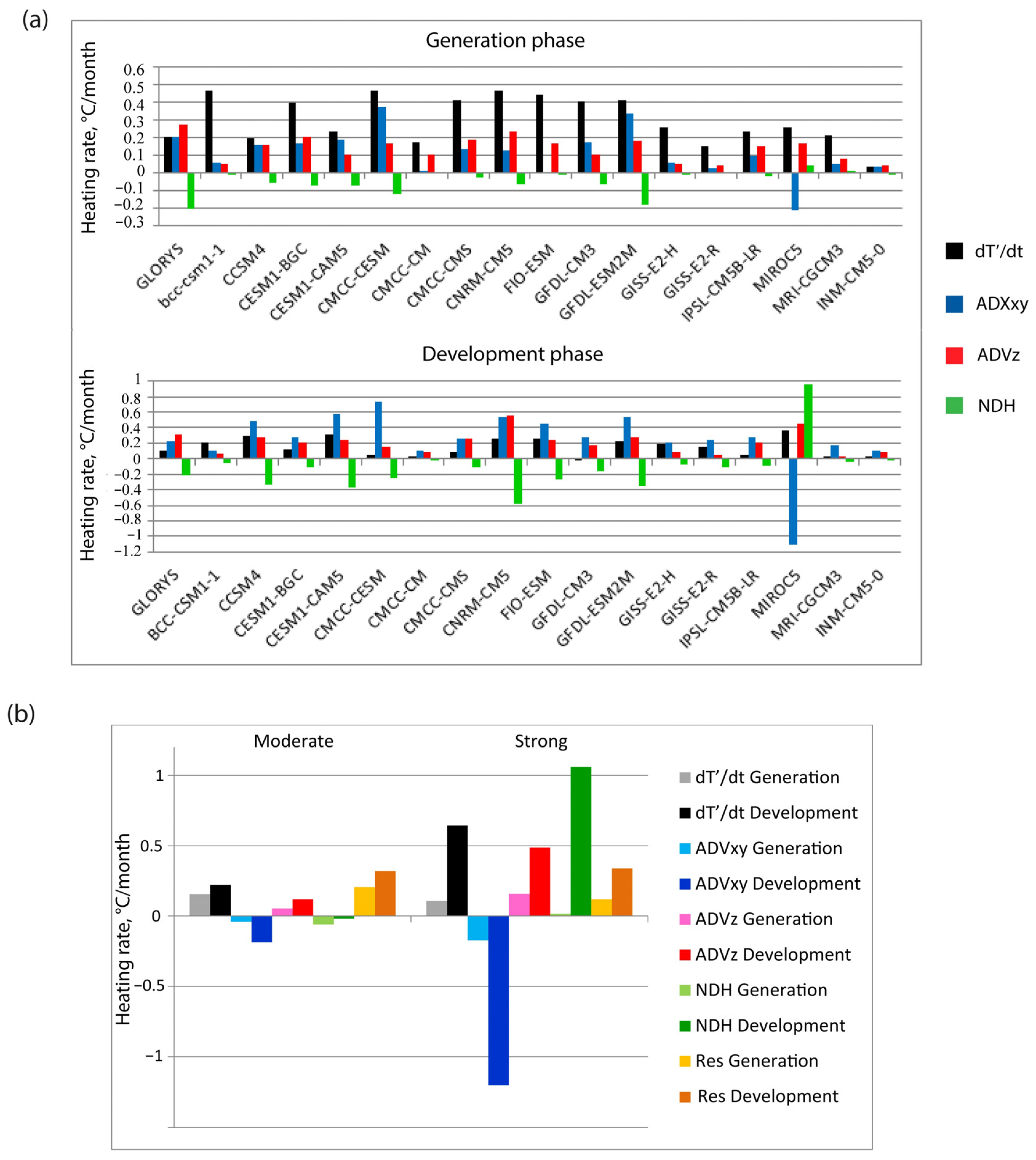
3.1. Observations
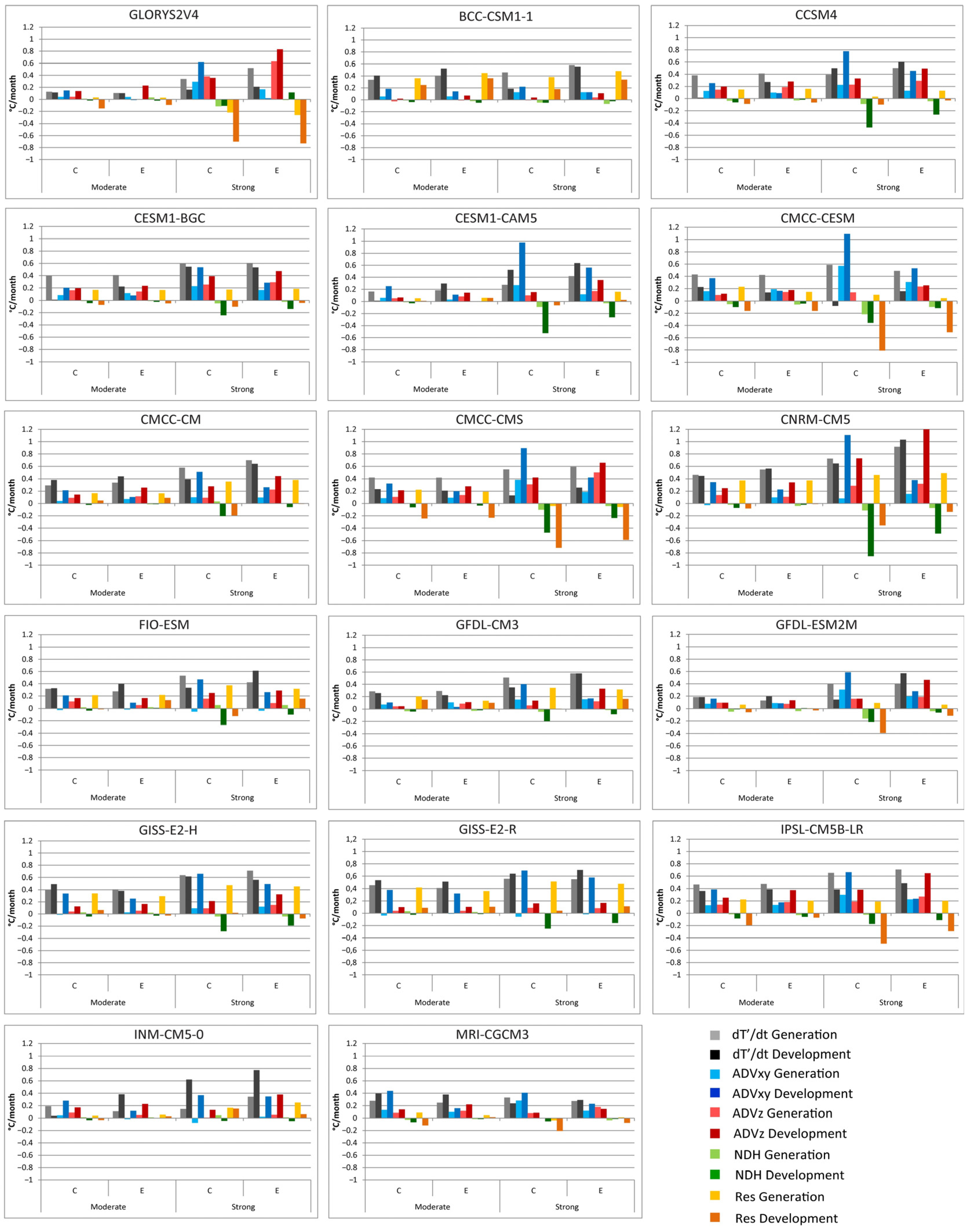
3.2. Models
4. Conclusions
Author Contributions
Funding
Institutional Review Board Statement
Informed Consent Statement
Data Availability Statement
Acknowledgments
Conflicts of Interest
References
- Ropelewski, C.F.; Halpert, M.S. Global and Regional Scale Precipitation Patterns Associated with the El Niño/Southern Oscillation. Mon. Weather Rev. 1987, 115, 1606–1626. [Google Scholar] [CrossRef]
- Trenberth, K.E.; Branstator, W.B.; Karoly, D.; Kumar, A.; Lau, N.C.; Ropelewski, C.F. Progress during TOGA in understanding and modeling global teleconnections associated with tropical sea surface temperatures. J. Geophys. Res. 1998, 103, 14291–14324. [Google Scholar] [CrossRef]
- Yeh, S.-W.; Cai, W.; Min, S.-K.; McPhaden, M.J.; Dommenget, D.; Dewitte, B.; Collins, M.; Ashok, K.; An, S.; Yim, B.; et al. ENSO atmospheric teleconnections and their response to greenhouse gas forcing. Rev. Geophys. 2018, 56, 185–206. [Google Scholar] [CrossRef]
- McPhaden, M.J.; Zebiak, S.E.; Glantz, M.H. ENSO as an integrating concept in earth science. Science 2006, 314, 1740–1745. [Google Scholar] [CrossRef]
- Cai, W.; Santoso, A.; Collins, M.; Dewitte, B.; Karamperidou, C.; Kug, J.-S.; Lengaigne, M.; McPhaden, M.J.; Stuecker, M.F.; Taschetto, A.S.; et al. Changing El Niño-Southern Oscillation in a warming climate. Nat. Rev. Earth Environ. 2021, 2, 628–644. [Google Scholar] [CrossRef]
- Rasmusson, E.M.; Carpenter, T.H. Variations in Tropical Sea Surface Temperature and Surface Wind Fields Associated with the Southern Oscillation/El Niño. Mon. Wea. Rev. 1982, 110, 354–384. [Google Scholar] [CrossRef]
- Ashok, K.; Behera, S.K.; Rao, S.A.; Weng, H.; Yamagata, T. El Niño Modoki and its possible teleconnection. J. Geophys. Res. 2007, 112, C11007. [Google Scholar] [CrossRef]
- Kao, H.-Y.; Yu, J.-Y. Contrasting Eastern-Pacific and Central-Pacific Types of ENSO. J. Clim. 2009, 22, 615–632. [Google Scholar] [CrossRef]
- Kug, J.S.; Jin, F.F.; An, S.I. Two types of El Niño events: Cold tongue El Niño and warm pool El Niño. J. Clim. 2009, 22, 1499–1515. [Google Scholar] [CrossRef]
- Takahashi, K.; Dewitte, B. Strong and moderate nonlinear El Niño regimes. Clim. Dyn. 2016, 46, 1627–1645. [Google Scholar] [CrossRef]
- Jin, F.-F.; Kim, S.T.; Bejarano, L. A coupled-stability index for ENSO. Geophys. Res. Lett. 2006, 33, L23708. [Google Scholar] [CrossRef]
- Zebiak, S.E.; Cane, M.A. A model El Niño–Southern Oscillation. Mon. Wea. Rev. 1987, 115, 2262–2278. [Google Scholar] [CrossRef]
- Choi, J.; An, S.-I.; Kug, J.-S.; Yeh, S.-W. The role of mean state on changes in El Niño’s flavor. Clim. Dyn. 2011, 37, 1205–1215. [Google Scholar] [CrossRef]
- Capotondi, A. ENSO diversity in the NCAR CCSM4 climate model. J. Geophys. Res. Oceans 2013, 118, 4755–4770. [Google Scholar] [CrossRef]
- Ren, H.-L.; Jin, F.-F. Recharge Oscillator Mechanisms in Two Types of ENSO. J. Clim. 2013, 26, 6506–6523. [Google Scholar] [CrossRef]
- Abellán, E.; McGregor, S.; England, M.H.; Santoso, A. Distinctive role of ocean advection anomalies in the development of the extreme 2015–2016 El Niño. Clim. Dyn. 2017, 51, 2191–2208. [Google Scholar] [CrossRef]
- Kug, J.S.; Choi, J.; An, S.-I.; Jin, F.-F.; Wittenberg, A.T. Warm pool and cold tongue El Niño events as simulated by the GFDL 2.1 coupled GCM. J. Clim. 2010, 23, 1226–1239. [Google Scholar] [CrossRef]
- Jin, F.-F.; An, S.-I.; Timmermann, A.; Zhao, J. Strong El Niño events and nonlinear dynamical heating. Geophys. Res. Lett. 2003, 30, 1120. [Google Scholar] [CrossRef]
- An, S.-I.; Jin, F.-F. Nonlinearity and Asymmetry of ENSO. J. Clim. 2004, 17, 2399–2412. [Google Scholar] [CrossRef]
- Kim, W.; Cai, W.; Kug, J.-S. Migration of atmospheric convection coupled with ocean currents pushes El Niño to extremes. Geophys. Res. Lett. 2015, 42, 3583–3590. [Google Scholar] [CrossRef]
- Santoso, A.; McPhaden, M.J.; Cai, W. The Defining Characteristics of ENSO Extremes and the Strong 2015/2016 El Niño. Rev. Geophys. 2017, 55, 1079–1129. [Google Scholar] [CrossRef]
- Carréric, A.; Dewitte, B.; Cai, W.; Capotondi, A.; Takahashi, K.; Yeh, S.-W.; Wang, G.; Guémas, V. Change in strong Eastern Pacific El Niño events dynamics in the warming climate. Clim. Dyn. 2020, 54, 901–918. [Google Scholar] [CrossRef]
- Garric, G.; Parent, L.; Greiner, E.; Drévillon, M.; Hamon, M.; Lellouche, J.M.; Régnier, C.; Desportes, C.; Le Galloudec, O.; Bricaud, C.; et al. Performance and quality assessment of the global ocean eddy-permitting physical reanalysis GLORYS2V4. In Proceedings of the EGU General Assembly, Vienna, Austria, 23–28 April 2017; Volume 19, p. 18776. [Google Scholar]
- Fedorov, A.V.; Philander, S.G. Is El Niño Changing? Science 2000, 288, 1997–2002. [Google Scholar] [CrossRef]
- DiNezio, P.N.; Kirtman, B.P.; Clement, A.C.; Lee, S.-K.; Vecchi, G.A.; Wittenberg, A. Mean Climate Controls on the Simulated Response of ENSO to Increasing Greenhouse Gases. J. Clim. 2012, 25, 7399–7420. [Google Scholar] [CrossRef]
- Fedorov, A.V.; Hu, S.; Lengaigne, M.; Guilyardi, E. The impact of westerly wind bursts and ocean initial state on the development, and diversity of El Niño events. Clim. Dyn. 2015, 44, 1381–1401. [Google Scholar] [CrossRef]
- Kim, S.T.; Cai, W.; Jin, F.-F.; Yu, J.-Y. ENSO stability in coupled climate models and its association with mean state. Clim. Dyn. 2014, 42, 3313–3321. [Google Scholar] [CrossRef]
- Karamperidou, C.; Jin, F.-F.; Conroy, J.L. The importance of ENSO nonlinearities in tropical pacific response to external forcing. Clim. Dyn. 2017, 49, 2695–2704. [Google Scholar] [CrossRef]
- Cai, W.; Wang, G.; Dewitte, B.; Lixin, W.; Santoso, A.; Takahashi, K.; Yang, Y.; Carréric, A.; McPhaden, M.J. Increased variability of Eastern Pacific El Niño under greenhouse warming. Nature 2018, 564, 201–206. [Google Scholar] [CrossRef]
- Takahashi, K.; Montecinos, A.; Goubanova, K.; Dewitte, B. ENSO regimes: Reinterpreting the canonical and Modoki El Niño. Geophys. Res. Lett. 2011, 38, L10704. [Google Scholar] [CrossRef]
- Takahashi, K.; Karamperidou, C.; Dewitte, B. A theoretical model of strong and moderate El Niño regimes. Clim. Dyn. 2018, 52, 7477–7493. [Google Scholar] [CrossRef]
- Hartigan, J.A.; Wong, M.A. Algorithm AS 136: A K-Means Clustering Algorithm. J. R. Stat. Soc. Ser. C Appl. Stat. 1979, 28, 100–108. [Google Scholar] [CrossRef]
- Dewitte, B.; Takahashi, K. Diversity of moderate El Niño events evolution: Role of air–sea interactions in the eastern tropical Pacific. Clim. Dyn. 2017, 52, 7455–7476. [Google Scholar] [CrossRef]
- Wang, G.; Cai, W.; Santoso, A. Stronger Increase in the Frequency of Extreme Convective than Extreme Warm El Niño Events under Greenhouse Warming. J. Clim. 2019, 33, 675–690. [Google Scholar] [CrossRef]
- Feng, M.; Hacker, P.; Lukas, R. Upper ocean heat and salt balances in response to a westerly wind burst in the western equatorial Pacific during TOGA COARE. J. Geophys. Res. Oceans 1998, 103, 10289–10311. [Google Scholar] [CrossRef]
- Wang, B.; Luo, X.; Sun, W.; Yang, Y.-M.; Liu, J. El Niño diversity across boreal spring predictability barrier. Geophys. Res. Lett. 2020, 47, e2020GL087354. [Google Scholar] [CrossRef]
- Pan, X.; Li, T.; Chen, M. Change of El Niño and La Niña amplitude asymmetry around 1980. Clim Dyn. 2020, 54, 1351–1366. [Google Scholar] [CrossRef]
- An, S.-I.; Jin, F.-F. Collective Role of Thermocline and Zonal Advective Feedbacks in the ENSO Mode. J. Clim. 2001, 14, 3421–3432. [Google Scholar] [CrossRef]
- Yu, J.; Li, T.; Jiang, L. Why Does a Stronger El Niño Favor Developing towards the Eastern Pacific while a Stronger La Niña Favors Developing towards the Central Pacific? Atmosphere 2023, 14, 1185. [Google Scholar] [CrossRef]
- Neelin, J.D.; Battisti, D.S.; Hirst, A.C.; Jin, F.-F.; Wakata, Y.; Yamagata, T.; Zebiak, S.E. ENSO theory. J. Geophys. Res. Oceans 1998, 103, 14261–14290. [Google Scholar] [CrossRef]
- Borlace, S.; Cai, W.; Santoso, A. Multidecadal ENSO amplitude variability in a 1000-yr simulation of a coupled global climate model: Implications for observed ENSO variability. J. Clim. 2013, 26, 9399–9407. [Google Scholar] [CrossRef]
- Jin, F.-F. An Equatorial Ocean Recharge Paradigm for ENSO. Part I: Conceptual Model. J. Atmos. Sci. 1997, 54, 811–829. [Google Scholar] [CrossRef]
- Su, J.; Zhang, R.; Li, T.; Rong, X.; Kug, J.-S.; Hong, C.-C. Causes of the El Niño and La Niña amplitude asymmetry in the equatorial eastern Pacific. J. Clim. 2010, 23, 605–617. [Google Scholar] [CrossRef]


| Model Name | Organization | City, Country | Number of Grid Cells | Number of Levels | |
|---|---|---|---|---|---|
| Longitude | Latitude | ||||
| BCC-CSM-1.1 | Beijing Climate Center (BCC), China Meteorological Administration (CMA) | Beijing, China | 360 | 232 | 40 |
| CCSM4 | National Center for Atmospheric Research (NCAR) | Boulder, Colorado, USA | 384 | 320 | 60 |
| CESM1-BGC | |||||
| CESM1-CAM5 | |||||
| CMCC-CESM | Centro Euro-Mediterraneo sui Cambiamenti Climatici/Euro-Mediterranean Center on Climate Change (CMCC) | Lecce, Italy | 182 | 149 | 31 |
| CMCC-CM | |||||
| CMCC-CMS | |||||
| CNRM-CM5 | Centre National de Recherches Meteorologiques (CNRM), Centre Europeen de Recherche et de Formation Avanceeen Calcul Scientifique (CERFACS) | Toulouse, France | 362 | 292 | 42 |
| FIO-ESM | The First Institute of Oceanography (FIO), State Oceanic Administration (SOA) | Qingdao, China | 320 | 384 | 40 |
| GFDL-CM3 | National Oceanic and Atmospheric Administration (NOAA), Geophysical Fluid Dynamics Laboratory (GFDL) | Washington, D.C.,USA | 360 | 200 | 50 |
| GFDL-ESM2M | |||||
| GISS-E2-H | National Aeronautics and Space Administration (NASA) Goddard Institute for Space Studies (GISS) | New York, USA | 144 | 90 | 26 |
| GISS-E2-R | 32 | ||||
| IPSL-CM5B-LR | Institut Pierre Simon Laplace (IPSL) | Guyancourt, France | 182 | 149 | 31 |
| MIROC5 | Japan Agency for Marine-Earth Science and Technology | Yokosuka, Japan | 256 | 224 | 50 |
| MRI-CGCM3 | Meteorological Research Institute (MRI) | Tsukuba, Japan | 368 | 360 | 51 |
| INM-CM5-0 | Institute of Numerical Mathematics (INM) | Moscow, Russia | 720 | 720 | 40 |
| Model Name | Total Number | Events Selected | Strong | Moderate | EP | CP | E-Index Threshold Values, °C |
|---|---|---|---|---|---|---|---|
| BCC-CSM1-1 | 51 | 40 | 7 | 16 | 13 | 6 | 1.6–1.7 |
| CCSM4 | 42 | 42 | 7 | 30 | 12 | 14 | 2.6–2.8 |
| CESM1-BGC | 41 | 38 | 7 | 17 | 11 | 10 | 1.8–2.3 |
| CESM1-CAM5 | 46 | 45 | 7 | 33 | 13 | 12 | 2.0–2.2 |
| CMCC-CESM | 38 | 35 | 4 | 21 | 9 | 9 | 2.0 |
| CMCC-CM | 39 | 35 | 3 | 21 | 12 | 3 | 2.7–3.3 |
| CMCC-CMS | 44 | 40 | 3 | 23 | 8 | 7 | 2.2–2.5 |
| CNRM-CM5 | 50 | 48 | 4 | 37 | 9 | 11 | 2.1–2.2 |
| FIO-ESM | 46 | 43 | 5 | 18 | 13 | 9 | 1.9 |
| GFDL-CM3 | 45 | 42 | 9 | 25 | 11 | 7 | 1.7–2.0 |
| GFDL-ESM2M | 36 | 36 | 11 | 13 | 12 | 12 | 1.5–2.1 |
| GISS-E2-H | 46 | 42 | 5 | 25 | 8 | 7 | 1.6–1.8 |
| GISS-E2-R | 45 | 40 | 7 | 19 | 19 | 7 | 1.5–2.2 |
| IPSL-CM5B-LR | 42 | 35 | 10 | 17 | 17 | 8 | 1.6–2.0 |
| MIROC5 | 33 | 30 | 3 | 21 | 7 | 12 | 1.7–2.7 |
| MRI-CGCM3 | 45 | 41 | 3 | 25 | 15 | 9 | 1.7–2.0 |
| INM-CM5-0 | 39 | 34 | 3 | 20 | 9 | 6 | 2.0–2.7 |
Disclaimer/Publisher’s Note: The statements, opinions and data contained in all publications are solely those of the individual author(s) and contributor(s) and not of MDPI and/or the editor(s). MDPI and/or the editor(s) disclaim responsibility for any injury to people or property resulting from any ideas, methods, instructions or products referred to in the content. |
© 2023 by the authors. Licensee MDPI, Basel, Switzerland. This article is an open access article distributed under the terms and conditions of the Creative Commons Attribution (CC BY) license (https://creativecommons.org/licenses/by/4.0/).
Share and Cite
Osipov, A.; Gushchina, D. The Heat Budget of the Tropical Pacific Mixed Layer during Two Types of El Niño Based on Reanalysis and Global Climate Model Data. Atmosphere 2024, 15, 47. https://doi.org/10.3390/atmos15010047
Osipov A, Gushchina D. The Heat Budget of the Tropical Pacific Mixed Layer during Two Types of El Niño Based on Reanalysis and Global Climate Model Data. Atmosphere. 2024; 15(1):47. https://doi.org/10.3390/atmos15010047
Chicago/Turabian StyleOsipov, Alexander, and Daria Gushchina. 2024. "The Heat Budget of the Tropical Pacific Mixed Layer during Two Types of El Niño Based on Reanalysis and Global Climate Model Data" Atmosphere 15, no. 1: 47. https://doi.org/10.3390/atmos15010047