Article

The Impact of an Oceanic Mesoscale Anticyclonic Eddy in the East China Sea on the Tropical Cyclone Yagi (2018)

1
Tianjin Navigation Instrument Research Institute, Tianjin 300131, China
2
National Marine Data and Information Service, Tianjin 300171, China
3
SGIDI Engineering Consulting (Group) Co., Ltd. Qingdao Branch, Qingdao 266199, China
*
Author to whom correspondence should be addressed.
Atmosphere 2024, 15(1), 81; https://doi.org/10.3390/atmos15010081
Submission received: 21 November 2023 / Revised: 27 December 2023 / Accepted: 4 January 2024 / Published: 9 January 2024
(This article belongs to the Special Issue Tropical Cyclones: Observations and Prediction)

Abstract

:
In August 2018, tropical cyclone (TC) Yagi rapidly intensified as it passed over an oceanic mesoscale anticyclonic eddy (eddy) in the East China Sea, increasing in TC intensity from a tropical storm to a severe tropical storm. The maximum surface wind speed increase (minimum sea level pressure decrease) of Yagi over sea surface temperature (SST) warm anomalies caused by the eddy accounted for 66.7% (36.4%) of the whole case. Regional atmospheric model experiments are conducted to aid the interpretations of the case of Yagi intensifying over the eddy. Model results indicate that the SST warm anomalies caused by the eddy increase and concentrate the heat flux transported from the ocean to the atmosphere, and the upper air warms up, which is conducive to the development of convection. As a result, the contribution of the eddy to TC enhancement is over 20% in the period over the eddy and the precipitation is more concentrated at the TC center. The model further showed that the eddy affects the TC, resulting in more favorable dynamic and thermal conditions around the TC after landfall for the formations of TC tornadoes.

1. Introduction

Tropical cyclones (TCs), which form over the tropical or subtropical oceans, are powerful and deep tropical weather systems characterized by intense warm-core cyclones rotating around low-pressure centers at mesoscale or synoptic scales [1]. The life cycle of TCs can be broadly categorized into four stages: formation, development, maturity, and decay. In observations, TCs are distinguished by huge vortex-structured cumuliform clouds [2,3]. During the mature stage, the typical TCs are about 100~2000 km in diameter, with the maximum surface wind speed (MSWS) exceeding 30 m s−1. Some intense TCs can even extend up to the upper troposphere and impose remarkable influences on the entire troposphere [4].
Each year, 70–100 named TCs form worldwide, with most of them occurring in summer and autumn [1]. Despite the improvements in weather forecasting and warning system, TCs are still a severe disaster, causing large numbers of fatalities and economic losses to coastal countries. Cyclone Nargis (2008), Super Typhoon Haiyan (2013), and Hurricane Maria (2017) claimed 138,000, 6329, and 3057 lives, respectively. In 2017, three major hurricanes struck the United States, resulting in a damage of $268 billion, which amounts for 60% of the U.S. annual GDP growth [5]. In China, the annual mean losses from TC disasters include 36.7 million affected people, 69.5 billion Yuan in direct economic losses, and 254 deaths [6]. Therefore, there is an urgent need to improve our understanding of TC’s processes.
Many celebrated studies have found that the background states of ocean and atmosphere are vital for the formation and development of TCs. It is widely accepted that the following thermal and dynamical conditions are essential for the TCs’ formation: warm sea surface temperatures (SST) above 26 °C to 60 m depth, a moist lower troposphere, the presence of Coriolis forces, weak tropospheric vertical wind shears, low-level relative vorticity, and initial convective disturbances [3,7]. In addition, the instability generated by the interactions between the cumulus convection and synoptic-scale disturbance, also known as the conditional instability of second kind (CISK), can reasonably explain the formation and sustainment of the TCs [8,9].
The oceans, as the fundamental factor determining the TCs’ intensification, provide the necessary energy and moisture for the deep convection and maintenance of TCs [10,11]. Previous studies have indicated that a SST in the range of 26~30 °C is conducive for the intensification of TCs, while the SST out of this range tends to slow down the TCs’ development [1,12]. Meanwhile, the presence of TCs, in turn, can influence the SST. The intense wind stress of TCs can spontaneously drive a cyclonic current pattern in the upper layer of the ocean, leading to the surface divergence and consequent upwelling of sea water, according to the Ekman pumping theory. Consequently, the colder deep water is pumped up to the sea surface, while the surrounding warmer water is sunk into the deeper ocean. Additionally, wind stress enhances the turbulent motion in the ocean, promoting a strong mixing of the surface and sub-surface waters. Under these influences, SST tends to decrease while the sub-surface temperature increases. As a result, the cooler SST inhibits the energy and moisture transported from the ocean towards atmosphere, which may suppress the TCs’ development and change the TCs’ path [13,14,15,16,17]. Besides warm SST, the oceanic mixed layer depth to 60 m is another overwhelming factor influencing the TCs [18,19], the thicker mixed layer promotes larger ocean heat content, which favors the energy and moisture transports from the ocean to the atmosphere, and thus leading to more intensified TCs [20].
There is an interaction between TCs and the ocean, so the atmosphere–ocean cou-pling model is an important research method. Fairall et al. (1996) introduced a bulk parameterization method for air–sea fluxes in the tropical ocean–global atmosphere coupled-ocean atmosphere response experiment [21]. Warner et al. (2010) developed the coupled ocean–atmosphere–wave–sediment transport (COAWST) modeling system, integrating multiple environmental factors [22]. Zambon et al. (2014) utilized the COAWST model to study Hurricane Ivan, providing insights into the application of the ocean-atmosphere-wave-sediment transport system in extreme weather events [23]. Ricchi et al. (2016) investigated an extreme cold air outbreak over the Adriatic Sea using a coupled ocean–atmosphere–wave model, analyzing the system’s performance under extreme meteorological conditions [24]. Meroni et al. (2018) emphasized the role of sea surface temperature patterns in modulating heavy midlatitude precipitation events [25]. In recent research, Ricchi et al. (2023) explored the impact of sea surface temperature and topography on the development of a large-hail storm event over the Adriatic Sea, highlighting the crucial role of the ocean–atmosphere–wave model in extreme weather events [26]. These studies collectively contribute in-depth insights into understanding the dynamics of ocean and atmosphere interactions, particularly regarding the applicability and performance of models under different meteorological conditions.
The oceanic eddies are typically accompanied with warm or cold cores of SST anomalies, which can have impacts on the generation and development of TCs. For instance, after passing through a warm eddy in the Gulf Stream, Hurricane Opal was rapidly enhanced, with its minimum sea level pressure (MSLP) dropping from 965 hPa to 916 hPa and MSWS increased from 49 m s−1 to 58 m s−1 [27]. The key reason for such intense enhancement is that the warm and deep oceanic mixed layer at the center of oceanic mesoscale anticyclonic eddy (eddy) can effectively suppress the cooling effect of TCs on the SST, and this favors the development of TC [28]. Lin et al. (2009) has pointed out that this intensification effect of warm eddies on TCs is also closely related with the duration of interaction, the strength of TCs and the scale of warm eddies [29]. In addition, warm eddies are of more importance to cold eddies in the TC’s development, as the quantity of TCs generated over the warm eddies is significantly larger than the TCs occurred over the cold eddies [30,31]. Thus, mesoscale eddies, especially warm eddies, are crucial for the generation and development of TCs. However, the extent to which eddies could modulate TCs remains unclear, which needs further investigation.
Landfalling TCs often spawn tornadoes—about 6% of the reported tornadoes in the United States originate within TC envelopes [32]. After a TC makes landfall, due to increased ground friction or cold air intrusion, some storm cells in the outer rain bands of a TC develop strongly, forming small supercell storms and triggering tornadoes [33]. The suitable convective available potential energy (CAPE), strong low-level wind shear, and lifting condensation level in the right front quadrant of a TCs direction are conducive to the formation of tornadoes [34]. Since eddies can affect a TC, it’s still unclear whether they could trigger the generations of tornadoes by changing the environment around a landing TC.
Tropical storm Yagi (International designation: 1814) initially formed 1330 km southeast of Hualien, Taiwan, at 00:00 UTC on 7 August 2018, and then moved north-westward and quickly intensified over the East China Sea. At around 15:35 UTC on 12 August, Yagi landed on the coast of Wenling, Zhejiang Province, China, with a MSWS of 28 m s−1 at its center. Influenced by the Yagi, heavy rainfall (100~150 mm day−1) and strong wind (>22 m s−1) occurred in some regions of the Shanghai, Zhejiang, Anhui, and Jiangsu Provinces, resulting in a total damage of Yagi including 2,373,000 affected people, 3 fatalities, and a direct economic loss amounting to 2.52 billion Yuan. In addition, 12 tornadoes emerged in Jiangsu and Shandong Provinces, triggered by the cyclonic circulation of Yagi, which also brought about severe loss [35].
During the rapid intensification of Yagi over the East China Sea, an eddy with a warm core happened to locate over the path of Yagi. Therefore, two natural questions arise from this phenomenon: (1) Does this eddy promote the deepening of Yagi? If the answer is yes, can we measure this effect quantitatively? (2) Are the tornadoes generated on land related with the forcing effect of Yagi? To address these issues, this paper evaluates the influences of the eddy on Yagi and focuses on the role of Yagi in triggering tornadoes after landing, by conducting and comparing the control and sensitivity experiments. The physical processes revealed in this study are helpful for future studies on TCs related to oceanic eddies.
Section 2 introduces the data and numerical model utilized in the study. The influences of the eddy on Yagi are presented in Section 3. In Section 4, we discuss the mechanisms through which the Yagi facilitates tornado generation. A summary and discussion are given in Section 5.

2. Data and Numerical Model

2.1. Data

The relevant data for the study of the strong tropical storm Yagi were obtained from the China Meteorological Administration (CMA) TC Best Track dataset, which is available for download from tcdata.typhoon.org.cn [36,37]. Through integrating satellite data, on-site observations, and reanalysis data, the dataset provides the position and intensity of TCs in the north-western Pacific Ocean, including the South China Sea, north of the equator and west of 180° E, at 6 h intervals since 1949. From 2018, the time frequency of TC Best Track dataset is increased to every 3 h during the 24 h prior to landfall in China and the period when the typhoon is active over Chinese land. The variables included in the dataset are: TC latitude and longitude, time, TC intensity, TC central minimum pressure, 2 min mean TC MSWS, and 2 min mean wind speed.
The reanalysis data used in this paper is the latest fourth-generation atmospheric reanalysis data ECMWF (European Centre for Medium-Range Weather Forecasts) Reanalysis v5 (ERA5) [38,39]. ERA5 is an improved version based on ERA-Interim, and it utilizes the integrated forecast system (IFS) four-dimensional data assimilation system developed by ECMWF. It assimilates various observational data, including land station measurements, ship-based observations and air sounding data. It has 137 sigma pressure layers in the vertical direction, with the highest layer reaching 0.01 hPa. The variables used in this paper include geopotential height, temperature, wind field, CAPE, and convective inhibition energy. The temporal resolution of ERA5 is 1 h and the spatial resolution is 0.25° × 0.25°.

2.2. The Numerical Model

The weather research and forecasting (WRF) model [40] v4.2 was utilized to simulate the processes of Yagi in this study. The outer and inner domains of the model adopt horizontal resolutions of 30 and 10 km, with a central location at (123° E, 35° N). The NCEP (National Centers for Environmental Prediction) GDAS/FNL 0.25 Degree Global Tropospheric Analyses and Forecast Grids final analysis data, available on a 0.25° × 0.25° grid, was utilized as the initial and lateral boundary conditions for the model. The bottom boundary conditions are from the Real Time Global (RTG) daily SST data [41] provided by NCEP, with a 0.083° × 0.083° grid. The simulation period started at 00:00 on 11 August 2018, which was 21 h before Yagi entered the warm water region. This provided ample time for the model to adapt, ensuring that the simulation results were not substantially biased by the considerable distance from the area of interest. The simulation ended at 15:00 on 12 August 2018, by which time the intensity of TC had already weakened, and no tornadoes were generated thereafter. The other parameter settings of the model are shown in Table 1.
To detect the impact of the eddy in the East China Sea on Yagi, we conducted two sets of experiments: a control run (CTL) with RTG SST, and a “no eddy” run (NoE) in which a 2D nine-point smoothing [51,52] was conducted on RTG SST 200 times to remove the warming effect of the eddy. By comparing the results of the CTL and the NoE runs, the impact of the eddy on Yagi could be explored.

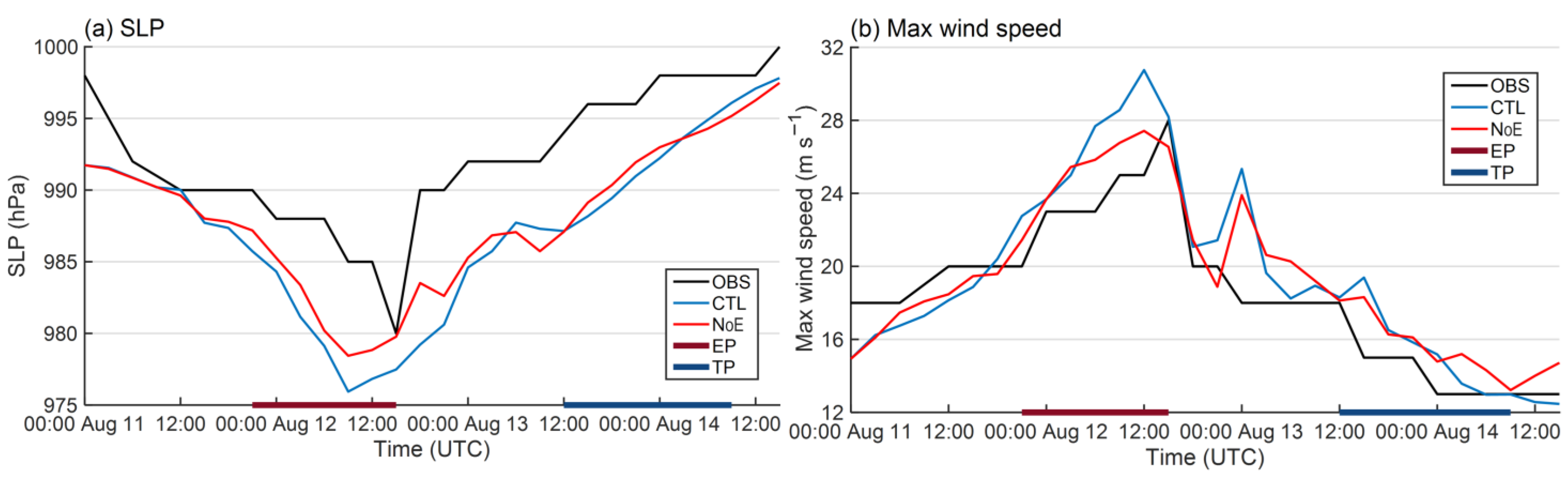
3. Impact of the Eddy on the Strength of TC Yagi

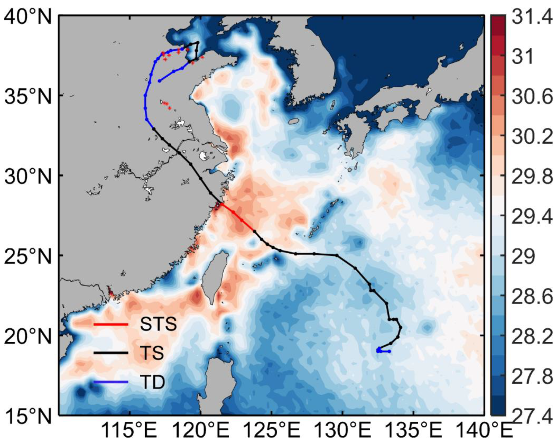
3.1. Overview of TC Yagi

TC Yagi formed at 06:00 UTC on 8 August 2018, in the north-west Pacific subtropical region, approximately 1330 km southeast of Hualien City, Taiwan (133.3° E, 19.0° N), which is shown in Figure 1. It started as a tropical depression with MSWS reaching 13 m s−1 and a MSLP of 1002 hPa. It initially moved quickly towards the west, then slowly developed for a day in place. Subsequently, it started moving towards the northeast at a speed of 10–15 km per hour. By this time, the TC Yagi had intensified into a tropical storm. At 18:00 UTC on 8 August, TC Yagi made a turn and started moving northwest. Over the next 30 h, its intensity remained relatively stable. However, after TC Yagi entered the East China Sea, its intensity started to increase. From Figure 1, it can be observed that compared to the Pacific east of Ryukyu Islands, the SST of the East China Sea was higher. Particularly in the nearshore area of southeastern Zhejiang Province, there was an eddy with SST warm anomalies diameter of about 200 km. After Yagi entered the eddy, the MSLP of Yagi decreased by 8 hPa, and MSWS increased by 8 m s−1. As a result, the intensity escalated from a tropical storm to a severe tropical storm. At 15:35 UTC on 12 August, Yagi landed at the coast of Wenling, Zhejiang Province. At the time of landing, MSWS reached 28 m s−1, and the MSLP was 980 hPa. After landing, the intensity of Yagi decreased to a tropical storm, with The MSWS reaching 20 m s−1. Yagi continued to move northwest at a speed of 35 km h−1. At 15:00 UTC on 13 August, its direction had shifted clockwise by approximately 40° in the Woyang area of Anhui Province. It then started moving in a northeast direction. At 21:00 UTC on 13 August, Yagi entered Shandong Province and weakened to a tropical depression. Subsequently, the tropical depression continued to move in a north-east direction. At 22:00 UTC on 14 August, it entered Bohai Sea from Hekou District, Dongying, Shandong Province. The decrease in friction on the underlying surface led to a further increase in the cyclone’s intensity, with central wind speed reaching 23 m s−1. Afterwards, it made a 180° turn in Laizhou Bay and re-landed from Weifang, Shandong Province at 12:00 UTC on 15 August, moving in a south-west direction. By 00:00 UTC on 16 August, it weakened and disappeared in Jining, Shandong Province.

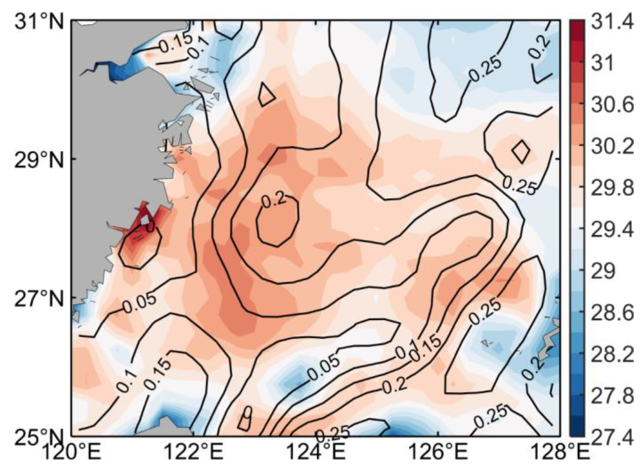
3.2. Development of Yagi near the Eddy Based on Observational Data

During the period of Yagi, there was an eddy with a sea surface height anomaly of 0.2 m over the eastern sea area of Zhejiang Province in the East China Sea (Figure 2). Under the influence of the closed eddy, a large area of high SST appeared over the East China Sea. Particularly on the western side of the eddy, SST reached 30.6 °C, which was more than 2 °C higher than SST in the Pacific east of Ryukyu Islands (Figure 1), due to the combined effects of horizontal and vertical flows. The anomalously high SST in the vicinity of the eddy resulted in an abnormally high heat flux from the ocean to the atmosphere. This contributed to the maintenance and development of the passing TC’s intensity.
Yagi entered the warm water region of the East China Sea from south-east at 21:00 UTC on 11 August and moved north-west (Figure 1). By 15:00 UTC on 12 August, Yagi landed on the coast of Wenling, Zhejiang Province. During the 18 h period when Yagi was moving over the warm water region influenced by the eddy, its MSLP decreased by 8 hPa, and the MSWS increased by 10 m s−1. As a result, the intensity of Yagi escalated from a tropical storm to a severe tropical storm (Figure 3). Within the 9 h period over the core region of SST anomalies, the MSLP of Yagi decreased by 5 hPa, and the MSWS increased by 8 m s−1. The pressure decrease (wind speed increase) over the SST anomalies region accounted for 36.4% (66.7%) of the total pressure decrease (wind speed increase) during the entire process of Yagi. Thus, it could be seen that the development of Yagi within this warm water region was a key for Yagi to become a severe tropical storm. In addition to the influence of the ocean, the large-scale circulation in background field also played an important role in the development of TC, factors such as weak vertical wind shears, favorable forcing from upper-level trough, and high relative humidity in the low-level atmosphere could all rapidly increase the intensity of TC that has not reached its maximum potential strength. Therefore, to understand the impact of SST anomalies caused by the eddy on the intensity of Yagi and separate it from the influences of atmosphere, only analyzing observational and reanalysis data is insufficient. Instead, numerical experiments were needed in this study.

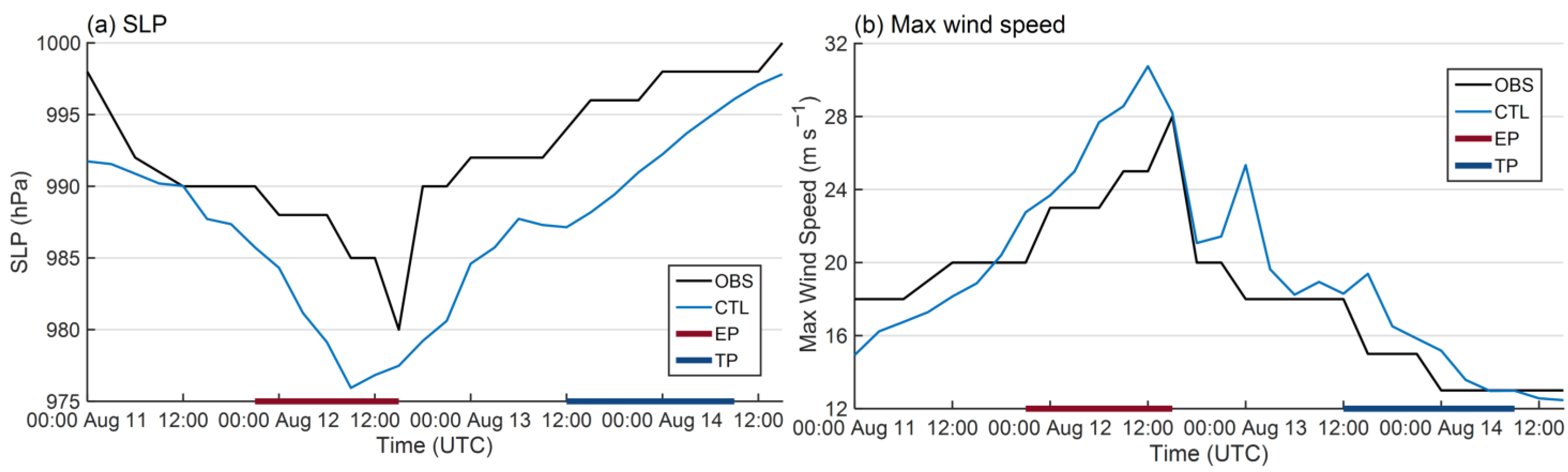
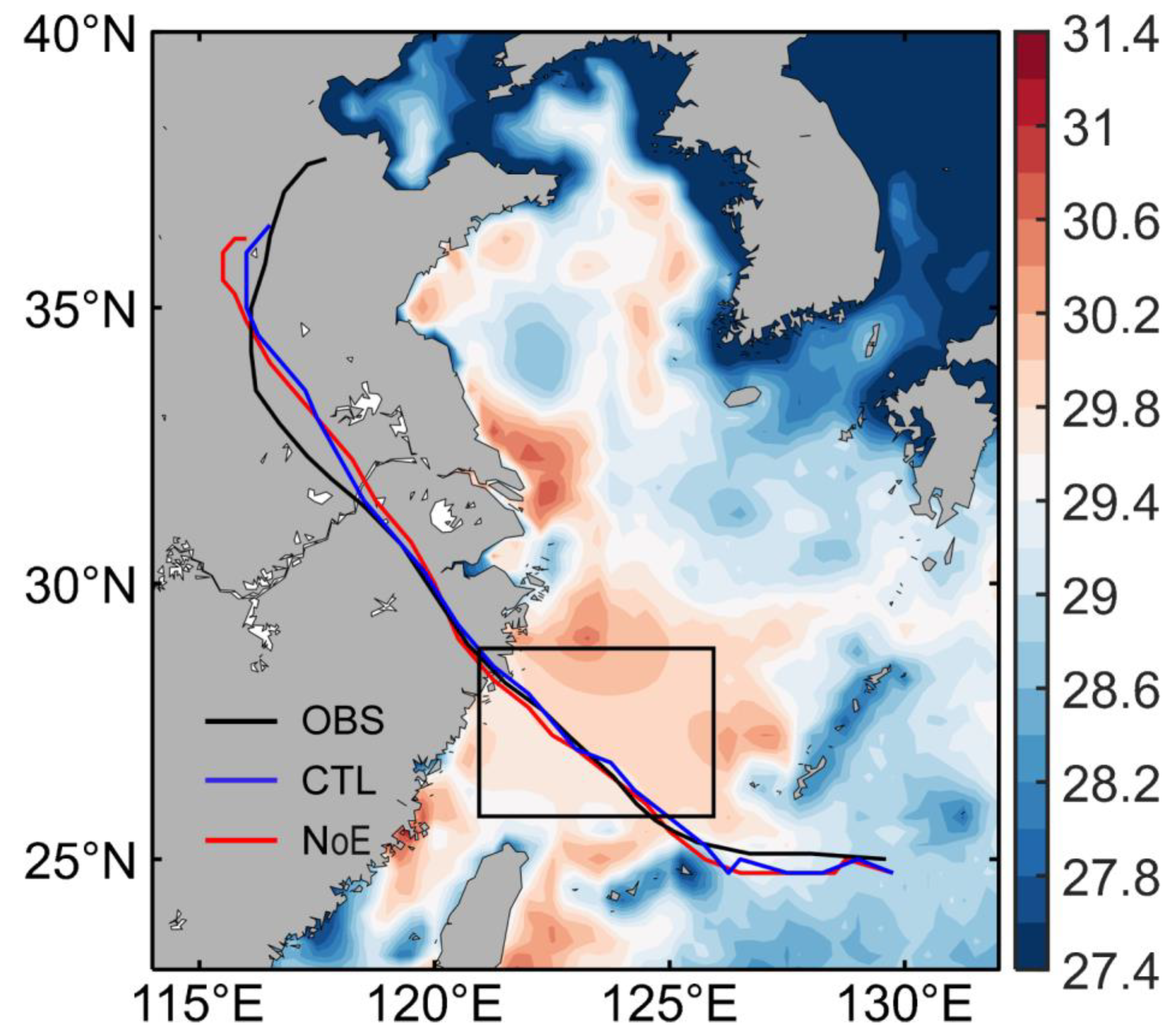
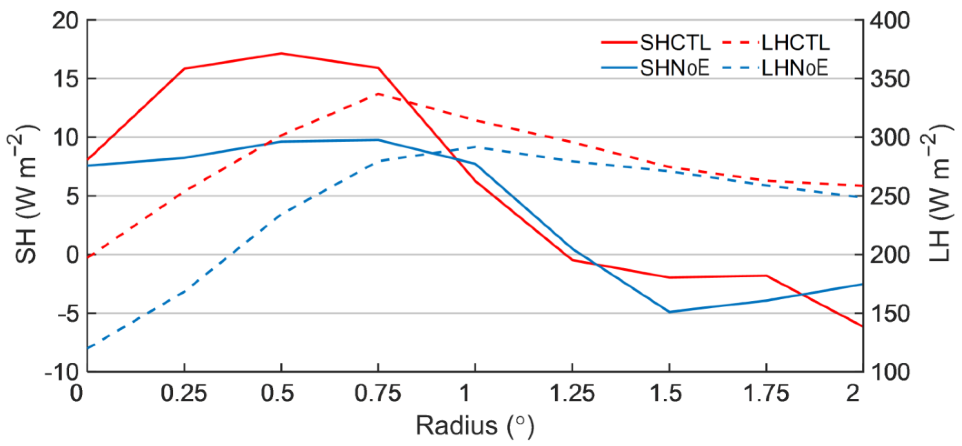
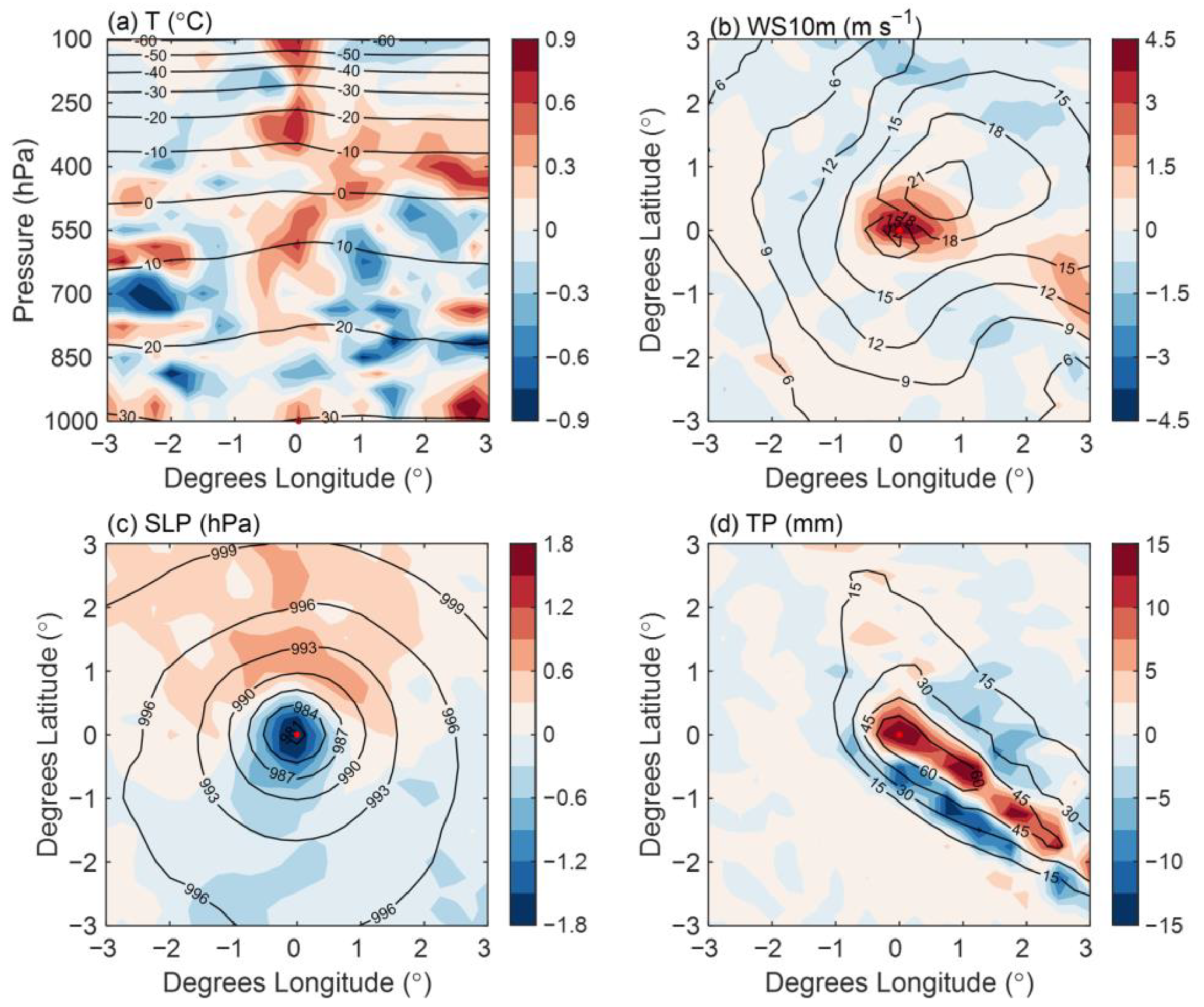
3.3. Impact of the Eddy on Yagi in Numerical Experiments

To investigate the impact of SST anomalies caused by the eddy on the intensity of Yagi, this study employed the well-established mesoscale meteorological model WRF to simulate the process of TC passing through the eddy. Sensitivity experiments were designed to explore the influence of the eddy on the intensity of Yagi.
First, the CTL is conducted using GDAS/FNL reanalysis data and RTG SST data to reproduce the process of TC passing through the eddy (for specific methods, see Section 3.2). By filtering the minimum values of sea level pressure at each time step in the results of the CTL, the simulated TC track is obtained as Figure 4, which generally agrees with the observed TC best track provided by CMA. During the initial 15 h of the simulation, there are certain fluctuations in the simulated path, which is the adjustment phase of the model. However, after the TC entered the warm water region, the simulated TC path basically consistent with the observed path, with an error within 0.5°. The simulated TC movement speed is slightly faster than the observation results, and this situation continued for 12 h after the landing of Yagi. After crossing the Yangtze River, the simulated path showed a deviation. The simulated path deviated from the observed path to the east with an error of within 1°. After entering Anhui Province, the simulated TC turned north-east, which aligned the path with the observed path. But with a time lag of 6 to 9 h. The simulation results shows that after the TC enters the warm water region caused by the eddy, the MSLP rapidly decreases by 10 hPa, slightly higher than the observed value of 8 hPa. The simulated TC reaches its maximum intensity about 3 h earlier than the observed time. The maximum intensity of simulated TC occurs at 12:00 UTC on 12 August, and the MSLP is 976 hPa, as shown in Figure 3a. After the TC lands, the atmospheric pressure starts to rise gradually. Comparing the simulation results with the observed data, it can be found that the MSLP at the TC center shows a similar trend in pressure changes. In addition, because the initial field value of sea level pressure input by the model is lower than the value given by CMA, which leads to the low pressure in the model simulation results during the whole process of TC development. But overall, the model well simulates the MSLP changes during the development of Yagi. In addition to the pressure of TC center, MSWS can also characterize the development in TC intensity. From Figure 3b, it can be observed that in the simulated results, after the TC enters the warm water region caused by the eddy, the maximum wind speed increases by 10 m s−1, slightly higher than the observed value of 8 m s−1. The time of maximum wind speed was at 12:00 UTC on 12 August, reaching a maximum of 31 m s−1, slightly higher than the observed value. After landing, the intensity of the TC gradually weakens, and MSWS decreases. As the TC moves from the mountainous region to the Middle–Lower Yangtze plains, the wind speed slightly increases, followed by another weakening. This trend is consistent with the wind speed changes reported by CMA. From the three aspects of TC path, the MSLP, and the MSWS, the results of the CTL successfully reproduce the rapid development of TC Yagi after entering the warm water region and the subsequent weakening and dissipation after landfall.
To investigate the impact of the eddy on the intensity changes of TC Yagi, this study designed sensitivity experiments (NoE) by smoothing the SST near the eddy in the initial field to remove the atmospheric responses of the eddy (for specific methods, see Section 2.2). After the smoothing process, the SST changes within the warm water area that TC passes are moderate, and the distinct SST fronts are no longer present. The SST anomalies caused by eddy are removed, as shown in Figure 4. Under such underlying surface conditions, the impacts of the eddy on the development of the TC are weakened. The results of NoE shows that the TC path is generally consistent with the CTL (shown in Figure 4), and the movement speed of TC remains basically unchanged. This indicates that the influences of the eddy on the path and the moving speed of the TC were relatively small. In terms of TC intensity, after the TC entered the region with smoothed SST, the MSLP (MSWS) continued to decrease (increase) rapidly, and the intensity of the TC increases (shown in Figure 5). However, after entering the core region of the SST anomalies, the development of TC intensity in the CTL significantly faster than the NoE (shown in Figure 5). At 12:00 UTC on 12 August, the TC intensity in both experiments reaches its maximum. In the NoE, the MSLP of the TC was 978 hPa, which was 2 hPa higher than the CTL, accounting for 20% of the pressure decrease in the CTL. MSWS in the NoE was 27 m s−1, which was 4 m s−1 lower than the CTL, accounting for 40% of the wind speed increase in the CTL. After TC landfall, the intensity of the TC in both runs were close. By comparing results in the CTL and the NoE, it can be found that the core area of SST warm anomalies caused by the eddy promotes the development of TC strength, with a contribution of 20% to 40%.
The SST anomalies caused by the eddy could change the atmospheric state by modifying the turbulent heat fluxes at the ocean-atmosphere interface, thus exerting impacts of the ocean on the atmosphere [52,53]. This study calculated the average heat fluxes near the TC center in the region affected by the eddy at various time steps, as shown in Figure 6. In terms of sensible heat flux, the maximum value of 17.2 (9.8) W m−2 is reached at 0.5° (0.75°) from the TC center in the CTL (NoE). In terms to latent heat flux, the maximum value of 337.1 (291.7) W m−2 is reached at 0.75° (1°) from the TC center in the CTL (NoE). The turbulent heat flux in the CTL is 52.8 W m−2 higher than that in the NoE and concentrates near the TC center. This indicates that the presence of the eddy could significantly increase the heat flux transferred from the ocean to the atmosphere near the TC center. The turbulent heat flux at the ocean-atmosphere interface is determined by variables such as the temperature difference between the ocean and the atmosphere, atmospheric humidity, and sea surface wind speed. When a TC passes through the SST warm anomalies caused by the eddy, the temperature difference between the ocean and the atmosphere increased, which is conducive to the increase in the heat flux transferred from the ocean to the atmosphere. In addition, the increase in wind speed around a TC caused by a warm eddy is also conducive to the increase in the heat flux transferred from the ocean to the atmosphere.
Under the influence of the SST warm anomalies caused by the eddy, the ocean transferred more heat to the atmosphere, providing the TC with additional energy and increasing its intensity [14]. To investigate the spatial distribution of the impact of the eddy on the TC, this study performed a composing analysis of the simulation results during the EP within a composing range of 300 km, which is typically the maximum radius reached by the TC rainbands. Figure 7 (shaded) shows the patterns of differences between CTL and NoE. Due to the convergence of warm water by the eddy, the high heat flux region is concentrated within a radius of 100 km from the TC center (Figure 6), and the corresponding warmer air above the TC center are also within this range (Figure 7a). In the CTL there is an obviously convex in the isotherm near the TC center. Compared to the results of NoE, the increase in temperature from 850 hPa to 100 hPa is more significant. The warm core structure is one of the most significant characteristics of TCs, and during TCs’ development, the warming of air is often be found in its upper atmosphere [54]. In the development process of a TC, the upper-level warm core has a more significant impact on reducing the sea surface pressure compared to the lower-level warm core [55]. According to the analysis of the high-altitude warm core in a case of TC, Wang et al. (2013) [56] suggested that the warm core formed by the increased upper atmospheric temperature caused by intense convection can enhance the rapid development of TCs. In the CTL, the stronger vertical convective mixing leads to more downward momentum transfer in this range, and the surface wind speed increases (Figure 7b). The variation of SLP is also concentrated near the TC center (Figure 7c), but its proportion of variation is smaller than that of wind speed. This indicates that during this process, vertical mixing plays a dominant role, and the effect of pressure adjustment is slightly weaker. During the EP, TC moves towards the north-west direction, so the precipitation caused by TC is within a band approximately 100 km wide to the southeast of the TC center in the composing results (Figure 7d). The precipitation in the CTL is 5–15 mm larger than that in the NoE within this band, while on both sides of this band, the precipitation in the CTL relatively less. This phenomenon may be attributed to the enhanced evaporation resulting from the increased SST in the region outside the eddy core after SST smoothing.

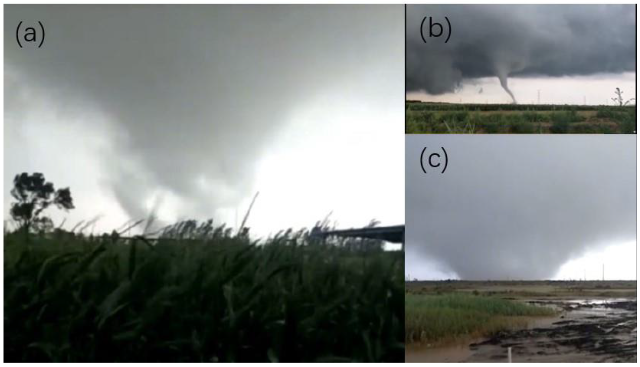
4. The Influence of Yagi on the Generation of Tornadoes

Yagi passed over the eddy and made landfall from Wenling, Zhejiang Province at 15:35 UTC on 12 August and moved northwest. When Yagi moved to the north of Anhui Province at 14:00 on 13 August, the first tornado was generated 160 km northeast of the TC center, near Xueji Village in Pizhou, Jiangsu Province, with an enhanced fujita (EF) scale [57] of 0 to 1. Later, when Yagi passed through the Shandong Province, 11 tornadoes with different intensities were generated in its vicinity (as shown in Figure 1 and Figure 8, Table 2). This was the highest recorded number of tornadoes generated by a TC landed in China. Consistent with the statistical results of distributions of TC tornadoes in the United States [32] and China [34], the tornadoes caused by the circulation of TC were all generated in the northeast quadrant of the TC center. The distance of these 12 tornadoes from TC center ranged from 100 to 360 km, with azimuth angles ranging from 35° to 75° in this case.
To explore the influence of Yagi on the generations of tornadoes in its vicinity, this study conducted a composite analysis of key meteorological variables near the TC center during the tornado generation period using ERA5 reanalysis data (Figure 3). It was known that large wind shear in the low level of troposphere could increase the risk of occurrence of TC tornados [58]. The storm relative helicity (SRH) associated with wind shear is a measure to reflect the strength of rotation within supercells and the extent of motion along the rotation axis. The calculation of SRH followed the formula introduced by [59]:
SRH = 0 H ( V h C ) · ( k × V h z ) d z
where H represents the given altitude, and V h is the horizontal wind speed, C is the storm motion, and k is the unit vector in the vertical direction. The SRH calculated from 0 to 3 km above the ground layer has been found to be a good parameter that can effectively characterize the potential of occurrence of tornadic supercells [60]. From Figure 9, it can be seen that there were high values of wind shear and SRH in the northeast of the TC center. The mechanical shear forces caused by large wind shear increased the instability of the atmospheric boundary layer, which promoted the development of convection. Although the magnitude of the maximum SRH during this process was only half of that observed in the TC tornadoes in the US [32], the maximum value of SRH at the northeast of the synthesized TC center reached 471 m² s−2 which was still 50% higher than the average value in the TC tornadoes in China (approximately 300 m² s²) [34]. In addition, the SRH based on the sounding data near TC tornadoes at 12:00 UTC on 13 August (00:00 UTC on 14 August), was 292 (276) m² s². It showed that within a range of 4° north-east of Yagi’s center was conducive to the dynamic conditions for supercells and tornados (Figure 9).
In the conditions for generations of TC tornados, thermal conditions are equally important as dynamical conditions. Due to the formation of TCs often accompanied by strong convection and the rise of warm and humid air, the instability of the atmosphere in the vertical direction increases. This instability makes it easier for potential energy in the atmosphere to be converted into convective energy, thereby increasing the CAPE value [32]. The instability generated by thermal processes was also conducive to the development of convection. In the research of tornados, one of the indicators used to evaluate the stability of the vertical atmospheric and the possibility of convection development was the CAPE, which was usually measured the likelihood of tornado generation [58]. CAPE represents the energy available to accelerate a parcel vertically. The calculation formula for CAPE is as follows:
CAPE = L F C E L g ( T V , p T V , e T V , e ) d z
where L F C represents the level of free convection. E L represents the equilibrium level. T V , p represents the virtual temperature of the lifted parcel. T V , e represents the virtual ambient temperature. g represents the gravitational acceleration. Figure 10a shows the CAPE near TC center calculated from ERA5 data. The area of high CAPE values is located north-east and south of the TC center, with a maximum value of 2100 J kg−1. The CAPE calculated from the sounding data near TC tornadoes at 12:00 UTC on 13 August (00:00 UTC on 14 August) is 1746 (1230) J kg−1. Although the CAPE value in the north-east quadrant was not high due to the low atmospheric pressure caused by the weakened TC, it also had the conditions for generations of tornados. The convective inhibition energy in the northern part of the TC was generally low, typically below 100 J kg−1. The calculated convective inhibition energy from the sounding data was only 10 and 76 J kg−1. This indicated that convection could effectively develop in the area where tornadoes generated. Additionally, the lifting condensation level of the TC center and its north-east area was relatively low (below 200 m), which was also conducive to tornados generations (Figure 10b).
In addition to the requirements of thermal and dynamical conditions, the generation of tornadoes also depends on favorable terrain. After landfall, Yagi first crossed the Southeast Hills, during which the northeast direction of the TC center had favorable thermal and dynamical conditions for tornado generation. However, due to the mountainous terrain in the vicinity, tornadoes were difficult to generate. Until Yagi entered the North China Plain, the tornado generated over flat farmland and wetlands in the Shandong and Jiangsu Provinces. Therefore, in addition to the influence of Yagi itself, the surrounding terrain also played an important role.
Miglietta et al. (2017) investigated the effect of SST on tornadoes generated at sea by conducting WRF experiments to alter SST [61]. The results indicate that variables such as CAPE, updraft helicity, absolute vorticity, etc., that characterize thermodynamic conditions around the tornado increase with the increase of SST (Figure 11), which is beneficial for the generation and development of tornadoes. Although the ocean did not directly affect the tornadoes during this case, the eddy could influence the formation of TC tornadoes by affecting the TC. Model experiments was used here to show the conditions differences around the TC. In the CTL, within a radius of 600 km from the center of the TC, especially in the northeast direction, the CAPE is significantly larger, with better thermal conditions for convection. The differences in dynamic conditions are mainly manifested at the center of the TC, with a radius of 200 km. In this case, 75% of TC tornadoes generated within 200 km north-east of Yagi’s center, therefore, the presence of the eddy was more conducive to the generation of TC tornadoes.

5. Discussion and Conclusions

In this study, we focused on the impact of an eddy in the East China Sea on the TC Yagi (2018). We used WRF to reproduce the process of Yagi intensifying over the eddy and the weakening of Yagi after landfall. Based on the reanalysis data and outputs from control and experiment WRF simulations, we found that the contribution of the eddy to Yagi enhancement was over 20% in the period over the eddy, the presence of the eddy made TC tornadoes easier to generate. Specific conclusions are:
TC Yagi passed over an eddy in the East China Sea, its MSLP (MSWS) decreased (increased) by 8 hPa (10 m s−1), with the intensity enhanced by tropical storms to a strong tropical storm. Comparisons of the results from CTL run and NoE run showed that the eddy could decrease (increase) the MSLP (MSWS) of Yagi by 2 hPa (4 m s−1) within a radius of 100 km from the center of the TC. The contribution of the eddy to Yagi enhancement exceeded 20% in the period over the eddy.
The eddy gathers the heat from the surrounding seawater at the warm anomalies center. Concentrated and increased heat flux from the ocean to the atmosphere at the warm anomalies center causes an abnormal rise of air temperature in the troposphere and a warm core appeared in the upper air, which promotes the development of convection. Under the dominance of vertical mixing, the proportion of changes in MSWS is greater than the decrease in MSLP. The concentrated latent heat flux and convection also leads to more precipitation in the TC center and less precipitation in the periphery.
During the tornado generation period, the north-east quadrant of the Yagi center had large wind shear and SRH, while the LCL was low, indicating that the dynamic and thermal conditions around Yagi were conducive to the generation of tornadoes. Numerical experiments showed that, when the eddy exists, the dynamic and thermal conditions within a radius of 200 km from the TC center are more favorable for tornadoes formations.
Due to the limited ability of WRF model to simulate small-scale processes [62], it is difficult to simulate tornadoes accurately, especially multiple tornadoes generated in one case of TC. Therefore, this study did not use numerical experiments to determine whether the eddy play a decisive role in TC tornado generation. But with the development of computer technology and observational technology, more in situ observations are assimilated, and high-resolution numerical simulations will help to continue this study.

Author Contributions

Conceptualization, J.S. (Jianxiang Sun) and J.S. (Jia Si); methodology, J.S. (Jianxiang Sun); software, J.S. (Jia Si) and J.C.; validation, J.S. (Jianxiang Sun), J.S. (Jia Si) and G.C.; formal analysis, J.S. (Jianxiang Sun) and D.Y.; investigation, J.S. (Jianxiang Sun) and G.C.; resources, H.L. and K.W.; data curation, J.C. and H.L.; writing—original draft preparation, J.S. (Jianxiang Sun) and J.S. (Jia Si); writing—review and editing, J.S. (Jianxiang Sun) and J.S. (Jia Si); visualization, J.S. (Jianxiang Sun) and K.W.; supervision, J.C.; project administration, J.S. (Jianxiang Sun); funding acquisition, J.S. (Jianxiang Sun), J.C. and G.C. All authors have read and agreed to the published version of the manuscript.

Funding

This research was funded by the National Key Research and Development Program of China (2021YFC3101605), and the National Natural Science Foundation of China (41976025).

Institutional Review Board Statement

Not applicable.

Informed Consent Statement

Not applicable.

Data Availability Statement

The data presented in this study are openly available. TC track data were acquired from CMA TC Best Track dataset (https://tcdata.typhoon.org.cn/zjljsjj.html accessed on 13 August 2022). The reanalysis data used in this paper is ERA5 from Copernicus Climate Change Service (C3S) Climate Data Store (CDS) (https://doi.org/10.24381/cds.adbb2d47, https://doi.org/10.24381/cds.bd0915c6 accessed on 18 August 2022). NCEP GDAS/FNL 0.25 Degree Global Tropospheric Analyses and Forecast Grids data (https://doi.org/10.5065/D65Q4T4Z accessed on 6 October 2022) and RTG SST data (https://polar.ncep.noaa.gov/sst/ophi/ 8 October 2022) were used for WRF running.

Conflicts of Interest

Jia Si, Kaiyue Wang and Huan Li are the employees of National Marine Data and Information Service. Dongren Yang is the employee of SGIDI Engineering Consulting (Group) Co., Ltd. The paper reflects the views of the scientists and not the company.

References

  1. Lin, J.L.; Qian, T.T.; Klotzbach, P. Tropical Cyclones. Atmos.-Ocean 2022, 60, 360–398. [Google Scholar] [CrossRef]
  2. Dvorak, V.F. Tropical Cyclone Intensity Analysis Using Satellite Data; US Department of Commerce, National Oceanic and Atmospheric Administration, National Environmental Satellite, Data, and Information Service: Washington, DC, USA, 1984; p. 11. [Google Scholar]
  3. Montgomery, M.T.; Farrell, B.F. Tropical cyclone formation. J. Atmos. Sci. 1993, 50, 285–310. [Google Scholar] [CrossRef]
  4. Sobel, A.H.; Camargo, S.J.; Hall, T.M.; Lee, C.Y.; Tippett, M.K.; Wing, A.A. Human influence on tropical cyclone intensity. Science 2016, 353, 242–246. [Google Scholar] [CrossRef] [PubMed]
  5. NOAA National Centers for Environmental Information (NCEI). State of the Climate: Hurricanes and Tropical Storms for Annual 2017. 2018. Available online: https://www.ncdc.noaa.gov/sotc/tropical-cyclones/201713 (accessed on 6 October 2022).
  6. Wang, H.; Xu, M.; Onyejuruwa, A.; Wang, Y.; Wen, S.; Gao, A.E.; Li, Y. Tropical cyclone damages in Mainland China over 2005–2016: Losses analysis and implications. Environ. Dev. Sustain. 2019, 21, 3077–3092. [Google Scholar] [CrossRef]
  7. Chang, C.P.; Liu, C.H.; Kuo, H.C. Typhoon Vamei: An equatorial tropical cyclone formation. Geophys. Res. Lett. 2003, 30, 1150. [Google Scholar] [CrossRef]
  8. Charney, J.G.; Eliassen, A. On the growth of the hurricane depression. J. Atmos. Sci. 1964, 21, 68–75. [Google Scholar] [CrossRef]
  9. Craig, G.C.; Gray, S.L. CISK or WISHE as the mechanism for tropical cyclone intensification. J. Atmos. Sci. 1996, 53, 3528–3540. [Google Scholar] [CrossRef]
  10. Palmen, E. On the formation and structure of tropical hurricanes. Geophysica 1948, 3, 26–38. [Google Scholar]
  11. Malkus, J.S.; Riehl, H. On the dynamics and energy transformations in steady-state hurricanes. Tellus 1960, 12, 1–20. [Google Scholar] [CrossRef]
  12. Chan, J.C.; Duan, Y.; Shay, L.K. Tropical cyclone intensity change from a simple ocean–atmosphere coupled model. J. Atmos. Sci. 2001, 58, 154–172. [Google Scholar] [CrossRef]
  13. Leipper, D.F. Observed ocean conditions and Hurricane Hilda. J. Atmos. Sci. 1967, 24, 182–186. [Google Scholar] [CrossRef]
  14. Lin, I.I.; Liu, W.T.; Wu, C.C.; Chiang, J.C.; Sui, C.H. Satellite observations of modulation of surface winds by typhoon-induced upper ocean cooling. Geophys. Res. Lett. 2003, 30, 1131. [Google Scholar] [CrossRef]
  15. Lin, I.I.; Wu, C.C.; Emanuel, K.A.; Lee, I.H.; Wu, C.R.; Pun, I.F. The interaction of Supertyphoon Maemi (2003) with a warm ocean eddy. Mon. Weather Rev. 2005, 133, 2635–2649. [Google Scholar] [CrossRef]
  16. Zhang, A.; Chen, Y.; Pan, X.; Hu, Y.; Chen, S.; Li, W. Precipitation microphysics of tropical cyclones over Northeast China in 2020. Remote Sens. 2022, 14, 2188. [Google Scholar] [CrossRef]
  17. Liu, T.; Chen, Y.; Chen, S.; Li, W.; Zhang, A. Mechanisms of the transport height of water vapor by tropical cyclones on heavy rainfall. Weather Clim. Extrem. 2023, 41, 100587. [Google Scholar] [CrossRef]
  18. Emanuel, K.; Nolan, D.S. Tropical cyclone activity and the global climate system. In Proceedings of the 26th Conference on Hurricanes and Tropical Meteorolgy, Miami, FL, USA, 3–7 May 2004; Volume 10, pp. 240–241. [Google Scholar]
  19. Wu, C.C.; Lee, C.Y.; Lin, I.I. The effect of the ocean eddy on tropical cyclone intensity. J. Atmos. Sci. 2007, 64, 3562–3578. [Google Scholar] [CrossRef]
  20. Leipper, D.F.; Volgenau, D. Hurricane heat potential of the Gulf of Mexico. J. Phys. Oceanogr. 1972, 2, 218–224. [Google Scholar] [CrossRef]
  21. Fairall, C.W.; Bradley, E.F.; Rogers, D.P.; Edson, J.B.; Young, G.S. Bulk parameterization of air-sea fluxes for tropical ocean-global atmosphere coupled-ocean atmosphere response experiment. J. Geophys. Res. Ocean. 1996, 101, 3747–3764. [Google Scholar] [CrossRef]
  22. Warner, J.C.; Armstrong, B.; He, R.; Zambon, J.B. Development of a coupled ocean–atmosphere–wave–sediment transport (COAWST) modeling system. Ocean Model. 2010, 35, 230–244. [Google Scholar] [CrossRef]
  23. Zambon, J.B.; He, R.; Warner, J.C. Investigation of hurricane Ivan using the coupled ocean–atmosphere–wave–sediment transport (COAWST) model. Ocean Dyn. 2014, 64, 1535–1554. [Google Scholar] [CrossRef]
  24. Ricchi, A.; Miglietta, M.M.; Falco, P.P.; Benetazzo, A.; Bonaldo, D.; Bergamasco, A.; Sclavo, M.; Carniel, S. On the use of a coupled ocean–atmosphere–wave model during an extreme cold air outbreak over the Adriatic Sea. Atmos. Res. 2016, 172, 48–65. [Google Scholar] [CrossRef]
  25. Meroni, A.N.; Parodi, A.; Pasquero, C. Role of SST patterns on surface wind modulation of a heavy midlatitude precipitation event. J. Geophys. Res. Atmos. 2018, 123, 9081–9096. [Google Scholar] [CrossRef]
  26. Ricchi, A.; Sangelantoni, L.; Redaelli, G.; Mazzarella, V.; Montopoli, M.; Miglietta, M.M.; Tiesi, A.; Mazzà, S.; Rotunno, R.; Ferretti, R. Impact of the SST and topography on the development of a large-hail storm event, on the Adriatic Sea. Atmos. Res. 2023, 296, 107078. [Google Scholar] [CrossRef]
  27. Bao, J.W.; Wilczak, J.M.; Choi, J.K.; Kantha, L.H. Numerical simulations of air–sea interaction under high wind conditions using a coupled model: A study of hurricane development. Mon. Weather Rev. 2000, 128, 2190–2210. [Google Scholar] [CrossRef]
  28. Jaimes, B.; Shay, L.K. Mixed layer cooling in mesoscale oceanic eddies during Hurricanes Katrina and Rita. Mon. Weather Rev. 2009, 137, 4188–4207. [Google Scholar] [CrossRef]
  29. Liu, G.P.; Hu, J.Y. The response of mesoscale eddies in the South China Sea to tropical cyclones: A case study. J. Oceanogr. Taiwan Strait 2009, 28, 8. [Google Scholar]
  30. Jangir, B.; Swain, D.; Ghose, S.K. Influence of eddies and tropical cyclone heat potential on intensity changes of tropical cyclones in the North Indian Ocean. Adv. Space Res. 2021, 68, 773–786. [Google Scholar] [CrossRef]
  31. Zhan, W.; He, Q.; Zhang, Y.; Zhan, H. Anticyclone Eddies Favor the Genesis of Off-Season Tropical Cyclone in the Western North Pacific. J. Geophys. Res. Atmos. 2023, 128, e2022JD036945. [Google Scholar] [CrossRef]
  32. Edwards, R. Tropical cyclone tornadoes: A review of knowledge in research and prediction. E-J. Sev. Storms Meteorol. 2012, 7, 1–61. [Google Scholar] [CrossRef]
  33. Novlan, D.J.; Gray, W.M. Hurricane-spawned tornadoes. Mon. Weather Rev. 1974, 102, 476–488. [Google Scholar] [CrossRef]
  34. Bai, L.; Meng, Z.; Sueki, K.; Chen, G.; Zhou, R. Climatology of tropical cyclone tornadoes in China from 2006 to 2018. Sci. China Earth Sci. 2020, 63, 37–51. [Google Scholar] [CrossRef]
  35. Zhu, J.J.; Cai, K.L.; Gong, D.L.; Liu, Y.; Wang, S.F.; Jin, W.F. Disaster investigation and weather radar identification of tornadoes in Shandong caused by landfalling Typhoon YAGI (2018). J. Mar. Meteorol. 2019, 39, 21–34. (In Chinese) [Google Scholar]
  36. Ying, M.; Zhang, W.; Yu, H.; Lu, X.; Feng, J.; Fan, Y.; Zhu, Y.; Chen, D. An overview of the China Meteorological Administration tropical cyclone database. J. Atmos. Ocean. Technol. 2014, 31, 287–301. [Google Scholar] [CrossRef]
  37. Lu, X.; Yu, H.; Ying, M.; Zhao, B.; Zhang, S.; Lin, L.; Bai, L.N.; Wan, R. Western North Pacific tropical cyclone database created by the China Meteorological Administration. Adv. Atmos. Sci. 2021, 38, 690–699. [Google Scholar] [CrossRef]
  38. Hersbach, H.; Bell, B.; Berrisford, P.; Biavati, G.; Horányi, A.; Muñoz Sabater, J.; Nicolas, J.; Peubey, C.; Radu, R.; Rozum, I.; et al. ERA5 hourly data on single levels from 1940 to present. In Copernicus Climate Change Service (C3S) Climate Data Store (CDS); 14 June 2018; Available online: https://cds.climate.copernicus.eu/cdsapp#!/dataset/reanalysis-era5-single-levels?tab=overview (accessed on 18 August 2022).
  39. Hersbach, H.; Bell, B.; Berrisford, P.; Biavati, G.; Horányi, A.; Muñoz Sabater, J.; Nicolas, J.; Peubey, C.; Radu, R.; Rozum, I.; et al. ERA5 hourly data on pressure levels from 1940 to present. In Copernicus Climate Change Service (C3S) Climate Data Store (CDS); 14 June 2018; Available online: https://cds.climate.copernicus.eu/cdsapp#!/dataset/reanalysis-era5-pressure-levels?tab=overview (accessed on 18 August 2022).
  40. Skamarock, W.C.; Klemp, J.B.; Dudhia, J.; Gill, D.O.; Liu, Z.; Berner, J.; Wang, W.; Powers, J.G.; Duda, M.G.; Barker, D.M. A Description of the Advanced Research WRF Model Version 4; National Center for Atmospheric Research: Boulder, CO, USA, 2019; p. 145. [Google Scholar]
  41. Thiébaux, J.; Rogers, E.; Wang, W.; Katz, B. A new high-resolution blended real-time global sea surface temperature analysis. Bull. Am. Meteorol. Soc. 2003, 84, 645–656. [Google Scholar] [CrossRef]
  42. Tao, W.; Joanne, S.; Michael, M. An Ice–Water Saturation Adjustment. Mon. Weather Rev. 1989, 117, 231–235. [Google Scholar] [CrossRef]
  43. Tao, W.; Wu, D.; Lang, S.; Chern, J.; Peters-Lidard, C.; Fridlind, A.; Matsui, T. High-resolution NU-WRF simulations of a deep convective-precipitation system during MC3E: Further improvements and comparisons between Goddard microphysics schemes and obser- vations. J. Geophys. Res. Atmos. 2016, 121, 1278–1305. [Google Scholar] [CrossRef]
  44. Pleim, J.E. A combined local and nonlocal closure model for the atmospheric boundary layer. Part I: Model description and testing. J. Appl. Meteorol. Climatol. 2007, 46, 1383–1395. [Google Scholar] [CrossRef]
  45. Grell, G.A.; Freitas, S.R. A scale and aerosol aware stochastic convective parameterization for weather and air quality modeling. Atmos. Chem. Phys. 2014, 14, 5233–5250. [Google Scholar] [CrossRef]
  46. Dudhia, J. Numerical study of convection observed during the winter monsoon experiment using a mesoscale two-dimensional model. J. Atmos. Sci. 1989, 46, 3077–3107. [Google Scholar] [CrossRef]
  47. Mlawer, E.J.; Taubman, S.J.; Brown, P.D.; Iacono, M.J.; Clough, S.A. Radiative transfer for inhomogeneous atmospheres: RRTM, a validated correlated-k model for the longwave. J. Geophys. Res. Atmos. 1997, 102, 16663–16682. [Google Scholar] [CrossRef]
  48. Tewari, M.; Chen, F.; Wang, W.; Dudhia, J.; Lemone, A.; Mitchell, E.; Ek, M.B.; Gayno, G.A.; Węgiel, W.; Cuenca, R.H. Implementation and verification of the unified Noah land-surface model in the WRF model. In Proceedings of the 20th Conference on Weather Analysis and Forecasting/16th Conference on Numerical Weather Prediction, Seattle, WA, USA, 14 January 2004. [Google Scholar]
  49. Park, S.; Bretherton, C.S. The University of Washington shallow convection and moist turbulence schemes and their impact on climate simulations with the Community Atmosphere Model. J. Clim. 2009, 22, 3449–3469. [Google Scholar] [CrossRef]
  50. Jiménez, P.A.; Dudhia, J.; González-Rouco, J.F.; Navarro, J.; Montávez, J.P.; García-Bustamante, E. A revised scheme for the WRF surface layer formulation. Mon. Weather Rev. 2012, 140, 898–918. [Google Scholar] [CrossRef]
  51. Jiang, Y.; Zhang, S.; Xie, S.; Chen, Y.; Liu, H. Effects of a Cold Ocean Eddy on Local Atmospheric Boundary Layer Near the Kuroshio Extension: In Situ Observations and Model Experiments. J. Geophys. Res. Atmos. 2019, 124, 5779–5790. [Google Scholar] [CrossRef]
  52. Wang, Q.; Zhang, S.P.; Xie, S.P.; Norris, J.R.; Sun, J.X.; Jiang, Y.X. Observed variations of the atmospheric boundary layer and stratocumulus over a warm eddy in the Kuroshio Extension. Mon. Weather Rev. 2019, 147, 1581–1591. [Google Scholar] [CrossRef]
  53. Sun, J.; Zhang, S.; Nowotarski, C.J.; Jiang, Y. Atmospheric Responses to Mesoscale Oceanic Eddies in the Winter and Summer North Pacific Subtropical Countercurrent Region. Atmosphere 2020, 11, 816. [Google Scholar] [CrossRef]
  54. Heymsfield, G.M.; Halverson, J.B.; Simpson, J.; Tian, L.; Bui, T.P. ER-2 Doppler radar investigations of the eyewall of Hurricane Bonnie during the Convection and Moisture Experiment-3. J. Appl. Meteorol. 2001, 40, 1310–1330. [Google Scholar] [CrossRef]
  55. Zhang, D.L.; Chen, H. Importance of the upper-level warm core in the rapid intensification of a tropical cyclone. Geophys. Res. Lett. 2012, 39, L02806. [Google Scholar] [CrossRef]
  56. Wang, Y.; Wang, H. The inner-core size increase of Typhoon Megi (2010) during its rapid intensification phase. Trop. Cyclone Res. Rev. 2013, 2, 65–80. [Google Scholar]
  57. Potter, S. Fine-tuning fujita. Weatherwise 2007, 60, 64–71. [Google Scholar] [CrossRef]
  58. McCaul, E.W., Jr. Buoyancy and shear characteristics of hurricane-tornado environments. Mon. Weather Rev. 1991, 119, 1954–1978. [Google Scholar] [CrossRef]
  59. Davies-Jones, R. Streamwise vorticity: The origin of updraft rotation in supercell storms. J. Atmos. Sci. 1984, 41, 2991–3006. [Google Scholar] [CrossRef]
  60. Sueki, K.; Niino, H. Toward better assessment of tornado potential in typhoons: Significance of considering entrainment effects for CAPE. Geophys. Res. Lett. 2016, 43, 12–597. [Google Scholar] [CrossRef]
  61. Miglietta, M.M.; Mazon, J.; Motola, V.; Pasini, A. Effect of a positive sea surface temperature anomaly on a Mediterranean tornadic supercell. Sci. Rep. 2017, 7, 12828. [Google Scholar] [CrossRef]
  62. Zheng, Y.G.; Liu, F.F.; Zhang, H.J. Advances in Tornado Research in China. Meteorol. Mon. 2021, 47, 1319–1335. (In Chinese) [Google Scholar]
Figure 1. The track of No. 14 tropical storm in 2018 Yagi and SST (shaded, unit: °C) in the sea on the east of China. Different colors represent different intensities. Red is a severe tropical storm, black is a tropical storm, and blue is a tropical depression.
Atmosphere 15 00081 g001
Figure 2. SST (shaded, unit: °C) and sea surface height anomaly (contour, unit: m) in the East China Sea on 11 August 2018.
Atmosphere 15 00081 g002
Figure 3. The changes of (a) MSLP and (b) MSWS of Yagi over the East China Sea and after landing. OBS: observation data; CTL: control run data; EP: eddy region period; TP: Tornado generation period.
Atmosphere 15 00081 g003
Figure 4. The track of TC and the smoothed SST (in black box, in °C) in the simulation results. OBS: observation data; CTL: control run; NoE: no eddy run.
Atmosphere 15 00081 g004
Figure 5. The changes of (a) MSLP and (b) MSWS of Yagi over the East China Sea and after landing. OBS: observation data; CTL: control run data; NoE: no eddy run data; EP: eddy region period; TP: Tornado generation period.
Atmosphere 15 00081 g005
Figure 6. Distribution of sensible heat flux (solid line) and latent heat flux (dashed line) near TC center in the CTL (red line) and the NoE (dashed line).
Atmosphere 15 00081 g006
Figure 7. Composites of CTL results (contour) of meteorological variables near TC center (red point) and composites of CTL results minus NoE results (shaded) during EP. (a) Sea level pressure; (b) 10 m high wind speed; (c) total precipitation; (d) air temperature.
Atmosphere 15 00081 g007
Figure 8. Funnel clouds caused by tornadoes were captured by meteorologists in (a) Mashihe village, Yanghu Town, Yangxin County, Binzhou City (117.40° E 37.53° N), (b) Tandong village, Yanwo Town, Lijin County, Dongying City (118.44° E, 37.68° N) and (c) Nanwang village, Liuhe street, Hekou District, Dongying City (118.47° E, 37.86° N) Available online: https://weibo.com/p/1005051763864272/home (accessed on 15 August 2022).
Atmosphere 15 00081 g008
Figure 9. Composites of surface to 3 km (a) wind shear and (b) SRH near TC Center (red spot) during tornado generation period in ERA-5 data.
Atmosphere 15 00081 g009
Figure 10. Composites of (a) CAPE (shaded), convective inhibition energy (contour) and (b) lifting condensation level near TC Center (red spot) during tornado generation period in ERA5 data.
Atmosphere 15 00081 g010
Figure 11. Composites of CTL results minus NoE results (shaded) during TP. (a) CAPE; (b) updraft helicity; (c) absolute vorticity.
Atmosphere 15 00081 g011
Table 1. Options of WRF-ARW.
ParametersGrid 1Grid 2
Grid spacing (km)3010
Grids130 × 130298 × 298
Center location123° E, 35° N
Number of vertical layers33
Time interval (hour)3
Micro physics optionsGoddard Scheme [42,43]
Planetary boundary layer physics optionsAsymmetric Convection Model 2 Scheme [44]
Cumulus parameterization optionsGrell–Freitas Ensemble Scheme [45]
Shortwave optionsDudhia Shortwave Scheme [46]
Longwave optionsRRTM Longwave Scheme [47]
Land surface optionsUnified Noah Land Surface Model [48]
Shallow cumulus optionsUniversity of Washington Scheme [49]
Surface layer optionsRevised MM5 Scheme [50]
SST updateon
Table 2. Information of tornadoes near TC Yagi (2018) [34,35].
Time (UTC)LocationEF ScaleThe Direction and Distance from the TC Center
14:30 13 August117.81° E, 34.21° N0~157°, 160 km
15:15 13 August117.44° E, 34.52° N0~150°, 153 km
16:25 13 August117.62° E, 34.48° N0~160°, 155 km
01:45 14 August119.44° E, 37.03° N0~165°, 290 km
02:30 14 August120.12° E, 37.38° N0~168°, 365 km
02:40 14 August119.08° E, 37.88° N0~152°, 308 km
04:10 14 August117.50° E, 37.25° N1~240°, 125 km
05:10 14 August117.40° E, 37.53° N0~135°, 114 km
05:20 14 August118.44° E, 37.68° N0~155°, 190 km
05:50 14 August117.36° E, 37.67° N0~132°, 99 km
06:00 14 August118.47° E, 37.86° N055°, 183 km
06:45 14 August117.77° E, 37.51° N0~154°, 110 km
Disclaimer/Publisher’s Note: The statements, opinions and data contained in all publications are solely those of the individual author(s) and contributor(s) and not of MDPI and/or the editor(s). MDPI and/or the editor(s) disclaim responsibility for any injury to people or property resulting from any ideas, methods, instructions or products referred to in the content.

