Article

Assessment of Different Boundary Layer Parameterization Schemes in Numerical Simulations of Typhoon Nida (2016) Based on Aircraft Observations

1
Southern Marine Science and Engineering Guangdong Laboratory (Zhuhai), School of Atmospheric Sciences, Sun Yat-sen University, Zhuhai 519082, China
2
Guangdong Provincial Key Laboratory of Regional Numerical Weather Prediction, Guangzhou Institute of Tropical and Marine Meteorology, China Meteorological Administration (CMA), Guangzhou 510080, China
3
Plateau Atmospheres and Environment Key Laboratory of Sichuan Province, College of Atmospheric Science, Chengdu University of Information Technology, Chengdu 610225, China
4
Guangxi Climate Center, Nanning 530000, China
5
Laboratory of Beihai National Climate Observatory, Nanning 530000, China
*
Authors to whom correspondence should be addressed.
Atmosphere 2023, 14(9), 1403; https://doi.org/10.3390/atmos14091403
Submission received: 2 August 2023 / Revised: 25 August 2023 / Accepted: 29 August 2023 / Published: 6 September 2023
(This article belongs to the Special Issue Tropical Cyclones: Observations and Prediction)

Abstract

:
This study aimed to find a boundary layer parameter scheme suitable for typhoons in the South China Sea based on a comparison with the aircraft detection data from Typhoon Nida (2016). We simulated the typhoon boundary layer wind field in different boundary layer schemes, such as YSU, MYNN, BouLac, and Shin-Hong, and with a no-boundary-layer parametrization scheme. The results were as follows: (1) In the eye and eyewall area, the YSU and MYNN schemes could better simulate the east–west wind characteristics and the YSU scheme could also simulate the jet current of the southerly wind component in the boundary layer in the eyewall. (2) Compared with the eye area, the easterly wind in the eyewall area was strong, and the overall vertical movement was weak. (3) The YSU and MYNN schemes had similar turbulent kinetic energies that were also similar to those from aircraft observations; the turbulent kinetic energy in the simulations of several schemes in the boundary layer was evidently lower than that in the aircraft observations. Thus, the MYNN and the YSU schemes yielded better simulations for the eye and eyewall areas, and the YSU scheme was more similar to the boundary layer observations.

1. Introduction

Typhoons are important severe weather systems that affect many countries, including China, and have a significant impact on social production, economic development, residents, and properties in China’s coastal areas [1]. The planetary boundary layer (PBL) scheme is responsible for vertical sub-grid-scale fluxes due to eddy transport throughout the entire atmospheric column, not just the boundary layer. The PBL scheme determines the flux profiles within the well-mixed boundary and stable layers, thus providing atmospheric tendencies for temperature, moisture (including clouds), and horizontal momentum in the entire atmospheric column. The Yonsei University (YSU) PBL parametrization is a non-local first-order parametrization that does not predict turbulent kinetic energy (TKE). Hong et al. (2006) [2] developed a parametrization by modifying the non-local closure parametrizations reported by Troen and Mahrt (1986) [3] and Hong and Pan (1996) [4]. They explicitly treated entrainment processes at the top of the PBL and include a correction to the local gradient, which incorporates the contributions of large-scale eddies to the total flux in the turbulence diffusion equations for prognostic variables. The MYNN2.5 and MYNN3 schemes are TKE-based schemes, where level 2.5 predicts the TKE as an extra prognostic variable, while level 3 adds variances in the potential temperature, moisture, and their covariances [5,6]. An additional option related to the MYNN PBL scheme is a wind farm parameterization that accounts for additional drag and turbulence generation by wind farm rotors [7]. This scheme is customizable for different rotor characteristics as a function of the wind speed. The BouLac PBL is a 1.5-order (level 2.5) scheme with a prognostic TKE equation and a method for calculating length scales that define both upward and downward length scales affected by the PBL top and ground; it uses the lesser of these for the length scale. Shin and Hong (2015) developed a scale-aware PBL option based on the YSU PBL scheme [8]. At larger grid sizes, it resembles the YSU scheme, but as the grid size becomes considerably smaller than the PBL depth, the non-local term decreases in strength to allow for the resolved scales to perform a fraction of the transport, consistent with the resolution.
Although there are many parameterization schemes for the boundary layer, based on observation alone, we must select the most practical scheme to improve simulations and predictions [7]. Presently, the literature contains numerous observational studies, but they are mostly based on ground observations in the Atlantic, Pacific, or coastal areas [9,10,11,12], with only a few focused on the South China Sea. Aircraft observation was recently performed by the Hong Kong Observatory, providing a complete view of the eyewall and eye area of the typhoon boundary layer with reliable data quality. Therefore, based on these observations, we constructed a set of experiments and found a parameter scheme suitable for typhoons in the South China Sea. The boundary layer characteristics of typhoons in the South China Sea are different from those in other sea areas, such as shallow interocean circulation [13], turbulence characteristics [14], and helical rolls [15] in the tropical cyclone boundary layer. Because different parameterization schemes for the boundary layer refer to different physical processes [16], the different physical features in the South China Sea possibly affect the choice of boundary layer schemes. In this study, we simulated Typhoon Nida (2016) using the weather research and forecasting (WRF) model, version 4.0, based on the National Centers for Environmental Prediction Final (NCEP-FNL) data, Integrated Multi-Satellite Retrievals for Global Precipitation Measurement (GPM) (IMERG) satellite data, the fifth generation European Centre for Medium-Range Weather Forecasts (ECMWF) reanalysis (ERA5) data, aircraft observations, and the China Meteorological Administration (CMA) best track data. We introduce our data and methods in Section 2. Numerical experiments on Typhoon Nida are presented in Section 3. Section 4 provides simulation assessments based on aircraft observations. Section 5 provides a summary and discussion of our findings.

2. Data and Methods

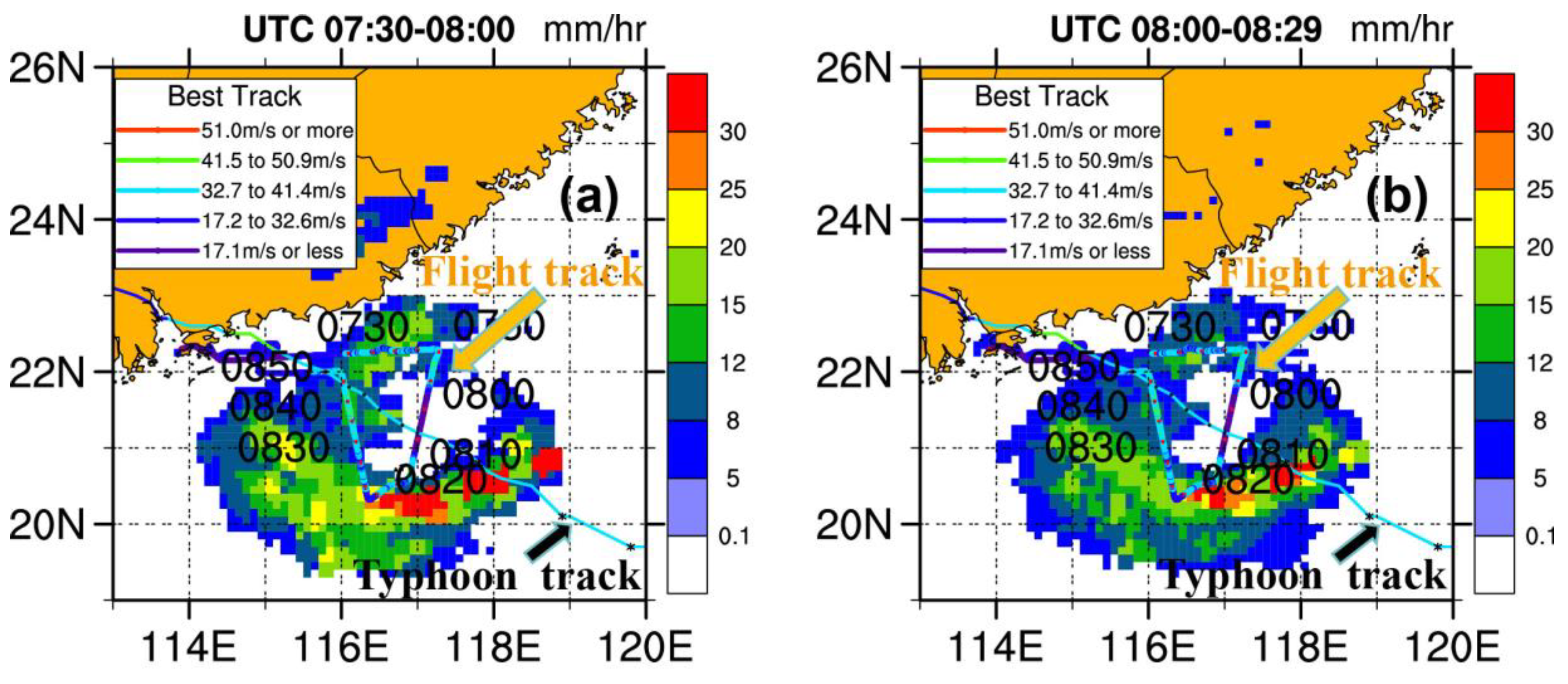
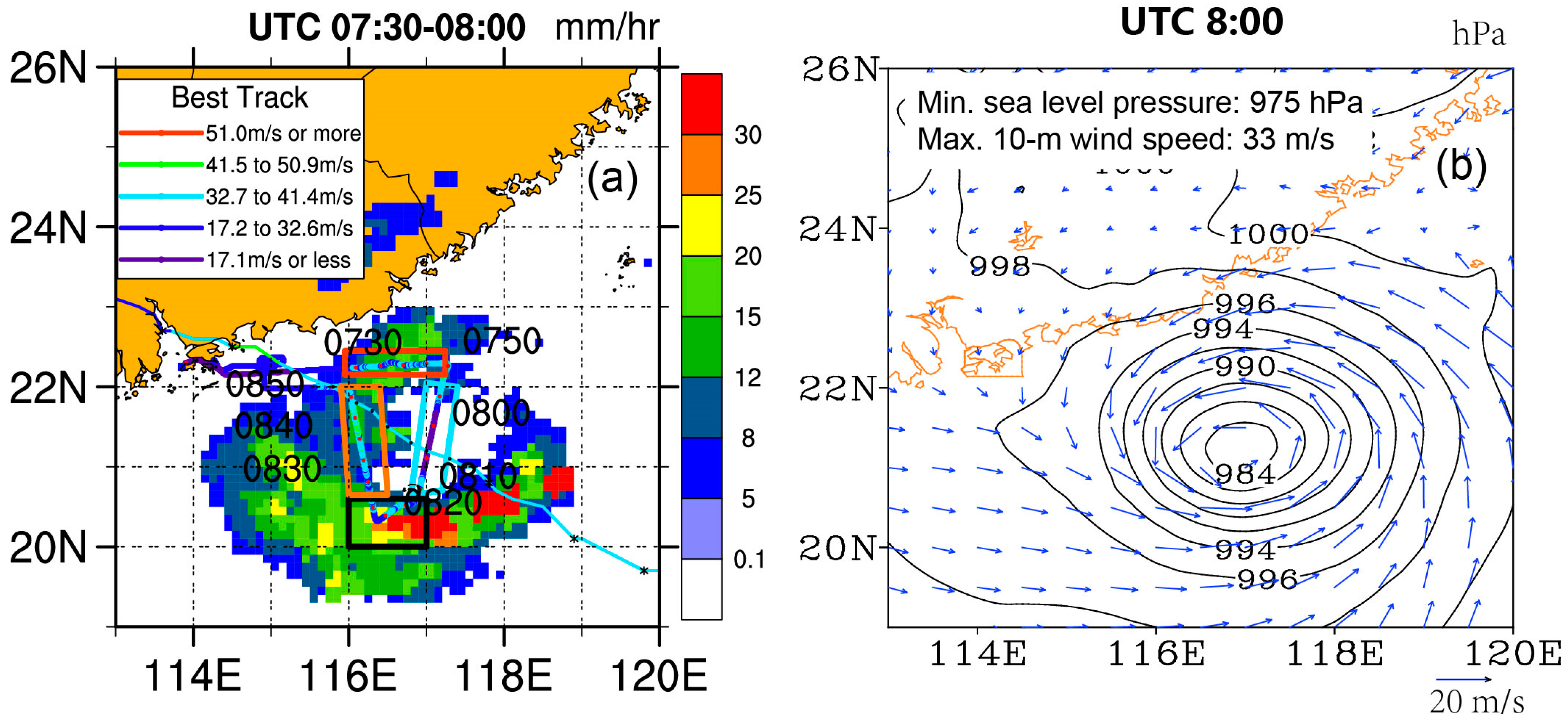
2.1. Aircraft Observations of Typhoon Nida

Observations were obtained from aircraft surveys performed jointly by the Hong Kong Observatory and the Hong Kong Government Flight Department using a Jetstream 4100 (J41) equipped with a 20 Hz Integrated Meteorological Measurement System (AIMMS-20) [17]. The post-processing of the original data by the AIMMS-20 measurement system improved the data quality [18]. The measurement accuracy after typical AIMMS-20 post-processing was improved by 20–30%. We selected the strong Typhoon Nida in 2016 as a case study. Because aircraft observations are mainly focused on the boundary layer, with an altitude of 1000 m approaching the boundary layer, and thus, we only selected the time when the altitude was below 1000 m [14].
Nida was generated at 6:00 on 30 July 2016 (UTC, the same below) at 127.3° E, 12.0° N. The generation intensity was at a tropical storm level, with a maximum wind speed of 20 m s−1, moving speed of 15 km h−1, air pressure of 995 hPa, and movement to the northwest. It intensified into a typhoon at 15:00 on 31 July, with a maximum wind speed of 33 m s−1, central pressure of 975 hPa, moving speed of 24 km h−1, and movement to the northwest. At 18:00 on 1 August, it reached its maximum intensity, i.e., a strong typhoon, at 115.1° E, 22.3° N. The maximum wind speed was 42 m s−1, with a central pressure of 960 hPa and a moving speed of 25 km h−1. At 20:00 on 1 August, it made landfall in Shenzhen, Guangdong, China, at typhoon intensity with a maximum wind speed of 40 m s−1 and a central pressure of 965 hPa. Based on the half-hour precipitation product from the Integrated Multi-Satellite Retrievals for GPM (IMERG), from a typhoon precipitation perspective (as shown in Figure 1), strong precipitation was mainly concentrated in the spiral rain belt on the south side. The precipitation range was 0–30 mm h−1 and the maximum precipitation reached 30 mm h−1. Precipitation on the north side was relatively weak, with a precipitation intensity of 5–20 mm h−1 and no notable precipitation near the typhoon eye.

2.2. Other Related Datasets

IMERG products provide precipitation measurements with high spatial (0.1° × 0.1°) and temporal (half-hourly) resolutions. There is a Level-3 dataset with three categories of output: the Early Run and Late Run consist of near-real-time monitoring products with delays of 6 and 18 h, respectively; the Final Run is a late-stage real-time research product with a 4-month delay. In this study, we used the Final Run products [19], which are available through NASA (http://pmm.nasa.gov/data-access/downloads/gpm, accessed on 31 August 2023). Final Run products were adjusted using monthly surface precipitation gauge estimates from weather stations [20]. The best track data were obtained from the CMA Tropical Cyclone (TC) Data Center (http://tcdata.typhoon.org.cn, accessed on 31 August 2023) [21]. NCEP-FNL is the final operational global analysis data from the Global Forecasting System of the National Centers for Environment Prediction. It is collected at 6 h intervals with global coverage and a horizontal resolution of 1° × 1° (http://rda.ucar.edu/datasets/ds083.2, accessed on 31 August 2023, ds083.2 | DOI: 10.5065/D6M043C6). ERA5 reanalysis data is available from the ECWMF (https://cds.climate.copernicus.eu/cdsapp#!/dataset/reanalysis-era5-single-levels?tab=form, accessed on 31 August 2023).

2.3. TKE

The instantaneous TKE [22] is estimated using 1 2 · u 2 + v 2 + w 2 , where u 2 , v 2 , and w 2 represent the pulsating velocities in the x, y, and z directions, respectively.

3. Model Design and Deviation Analysis

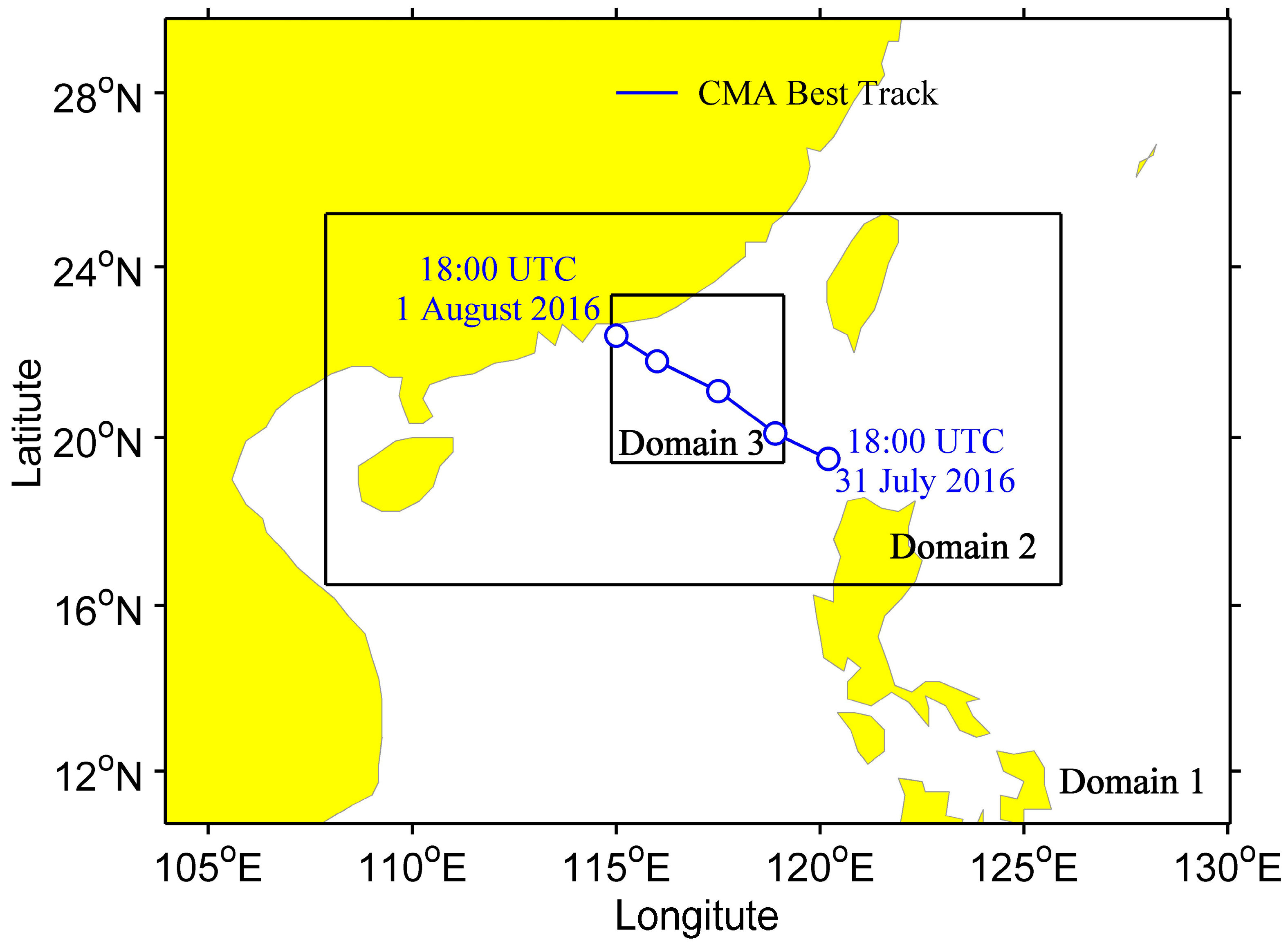
3.1. Model and Experimental Design

The model domain covered South Asia and the South China Sea (2.79° N to 21.37° N, 109.88° E to 162.11° E) (Figure 2). The initial and boundary conditions were obtained from the NCEP-FNL reanalysis data [23].
The 24 h simulations of Nida (18:00 UTC on 31 July 2016, to 18:00 UTC on 1 August 2016) were carried out using the advanced WRF (WRF-ARW) model version 4.0 [24] in a two-way interactive manner with triply nested domains at horizontal resolutions of 4.5, 1.5, and 0.5 km. The parameterization scheme settings are shown in Table 1 and Table 2. In terms of the height coordinates, the lowest 11 levels were within an altitude of 2 km from the surface. All sensitivity experiments were conducted at the time when the storm was over the ocean. At the same time, to simulate the turbulence in high resolution, we used four nested layers with the same parameter settings, but the grid resolutions were 2.7, 0.9, 0.3, and 0.1 km.

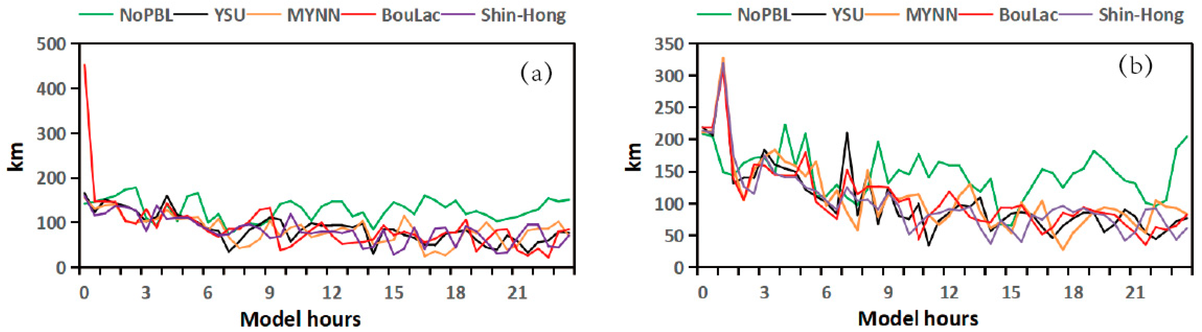
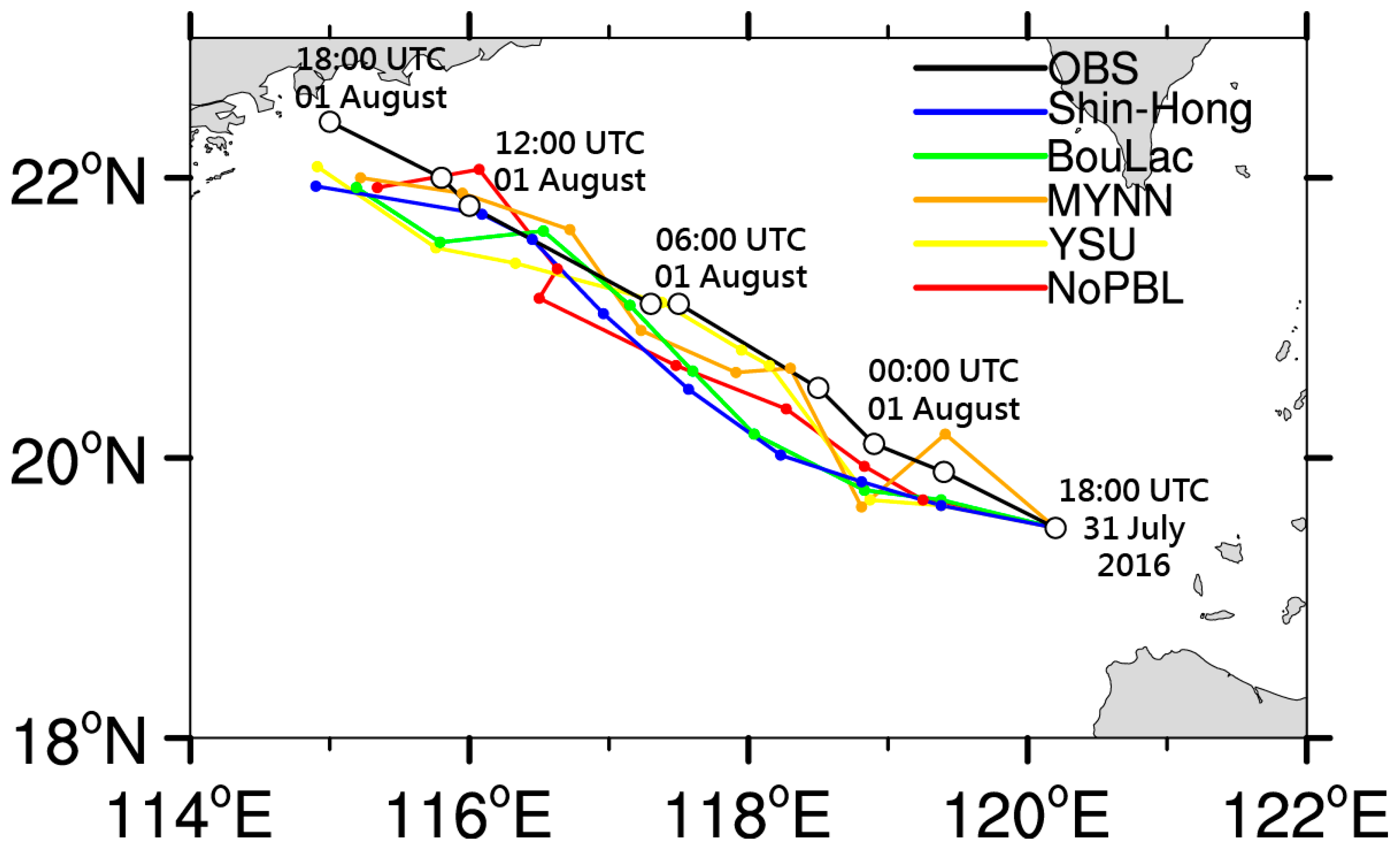
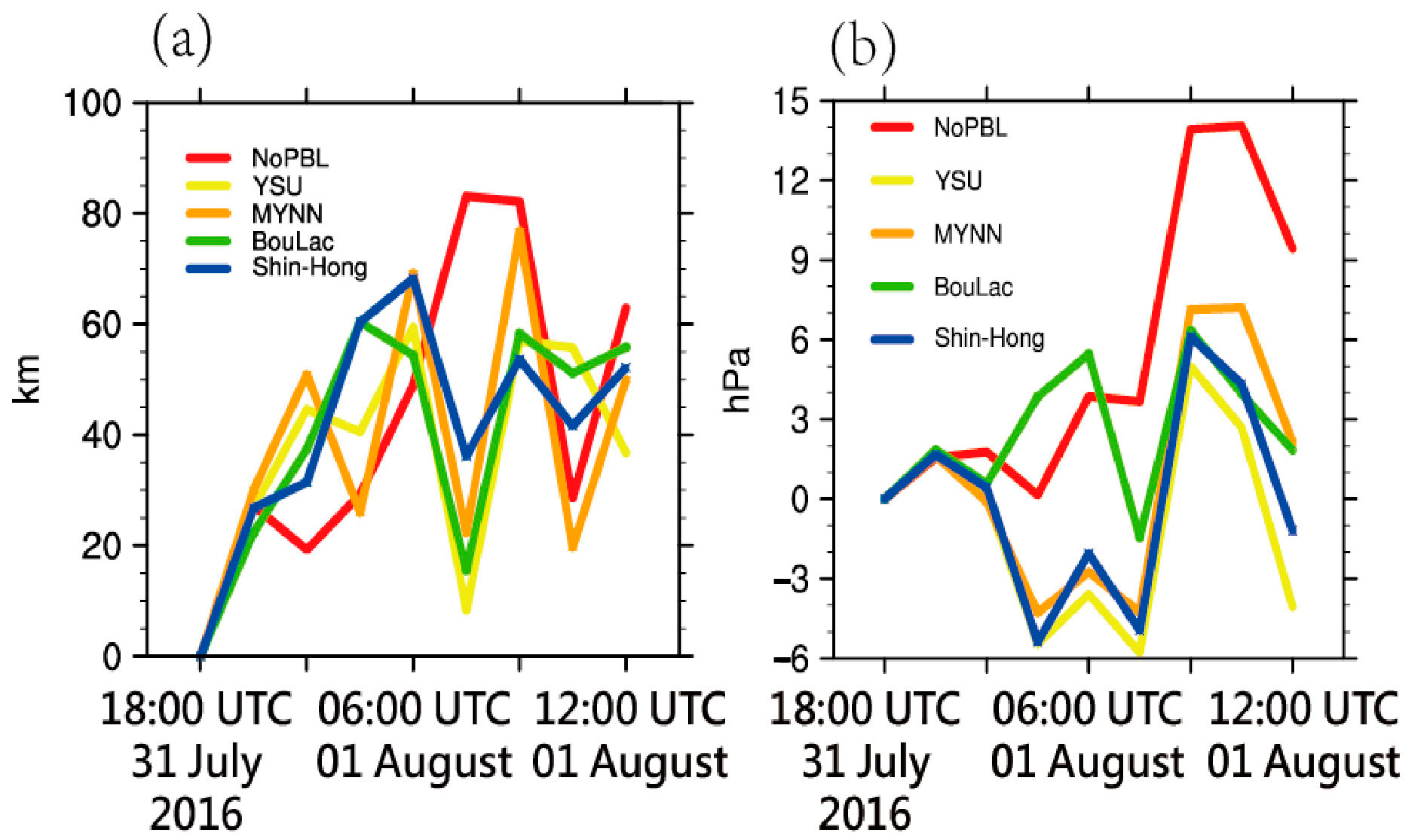
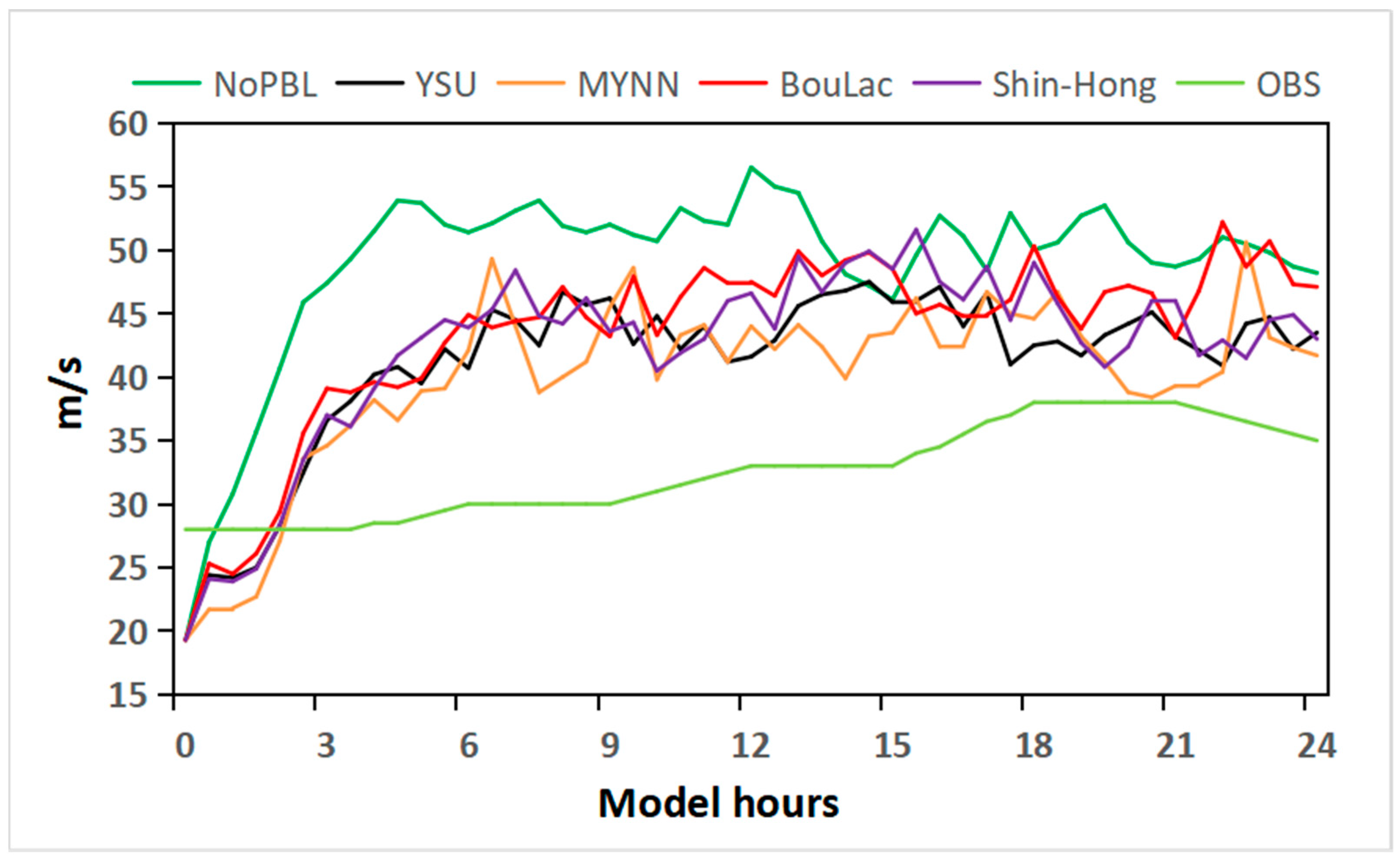
3.2. Simulated Deviation Analysis

Before model hour 7, the maximum wind radius of the TC significantly shrunk at sea level and an altitude of 6.0 km (Figure 3). Since the present study mainly focused on the typhoon boundary layer structure, especially the strong convective cloud tower, we thus preferred to analyze the maximum wind radius of the TC at sea level and an altitude of 6.0 km rather than the central intensity of the typhoon. To examine the characteristics of a stable TC evolution, we focused on the results from the model hours 7–9 (analyzed period) [25].
We divided the analysis areas of Typhoon Nida into four parts based on the track of aircraft observation and the eyewall structure based on the distribution of precipitation, sea level pressure, and low layer winds, as shown in Figure 4, i.e., the weak eyewall area on the north side (area I; analysis period: 7:30–7:50), eye area (area II; analysis period: 7:50–8:10), deep convection area on the south side (area III; analysis period: 8:10–8:30), and weak eyewall area on the west side (area IV; analysis period: 8:30–8:55).
Generally, all parameterization schemes could simulate the basic structure of the typhoon, with certain simulation effects on the precipitation, wind field, and pressure field. The parameterization scheme with the boundary layer had better simulation effects than the parameterization scheme without the boundary layer (better simulation of the typhoon spiral rain band and eye area), especially with the YSU scheme. The path simulation (Figure 5 and Figure 6a) with the YSU scheme had the best result (mean deviation of 36.6 km), while NoPBL (scheme without boundary layer parameterization) had the worst result (mean deviation of 42.38 km). The intensity aspect contained both pressure and wind speed: the better pressure simulations (Figure 6b) were the YSU, MYNN, and Shin-Hong schemes, especially the Shin-Hong scheme, which had the best effect (mean deviation of −0.11 hPa), whereas NoPBL had the worst effect (mean deviation of 5.38 hPa). The YSU (7.6 m s−1) and MYNN schemes (7.0 m s−1) had the best wind speed simulations (Figure 7), while NoPBL had the worst (average deviation of 14.3 m s−1). For precipitation (Figure 8), the YSU scheme was the best (i.e., the area ratio of each rainfall class and percentage of rainfall in each class were similar to the actual situation), while the NoPBL scheme was the worst (i.e., the ratio of the area occupied by each class of rainfall and percentage of rainfall in each class deviated markedly from the actual situation). It is worth noting that the NoPBL scheme overestimated the wind speed but underestimated the precipitation. The possible reason was that the spatial distribution of the low layer divergence, which is one of the important factors of precipitation, was modified by the changed winds. This should be further studied and analyzed in the future.

4. Simulation Assessment Based on Aircraft Observations

The forecasting capability of the numerical model was reflected in the degree of temporal and spatial refinement and accuracy of the forecast elements. The wind field forecast was especially the most important; the difference in the spatial distribution in the vertical direction could best reflect the characteristics of the numerical model. For example, the simulation of the V-wind showed that there was a clear north–south wind transition, with a leftward tilt from the lower to upper levels. This unique spatial distribution characteristic of the eye area was beneficial to our further understanding of the water vapor, energy, and momentum transport and exchange in typhoons. The vertical motion in the typhoon eye area was stronger than the general convective activity. The strength of the vertical motion reflected the degree of energy, momentum, and water vapor exchange within the typhoon system. In this section, we compared the numerical simulations (Figure 9, Figure 10, Figure 11, Figure 12, Figure 13, Figure 14, Figure 15 and Figure 16) to the observations (Figure 15 and Figure 16 and Table 3) as follows.

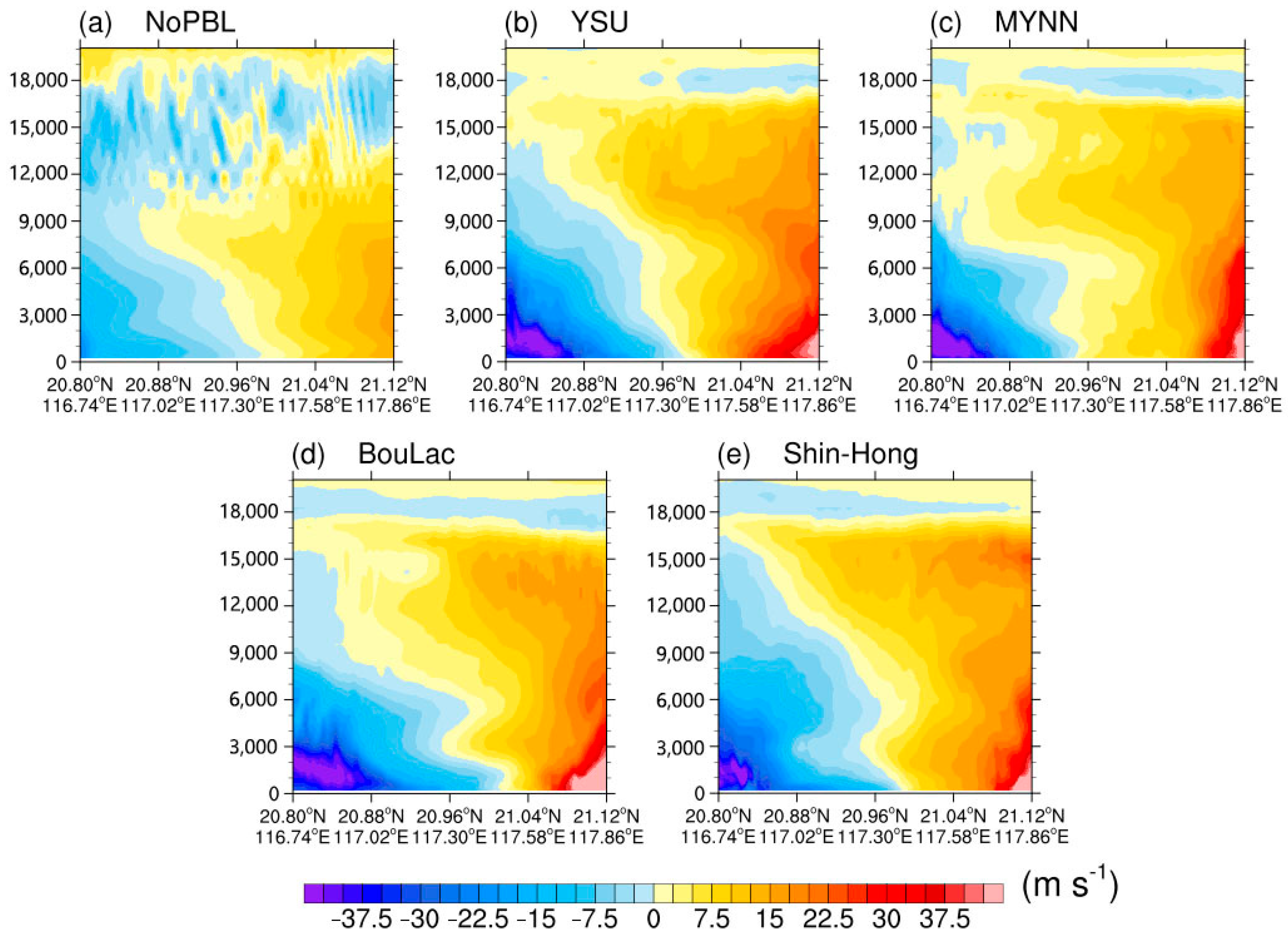
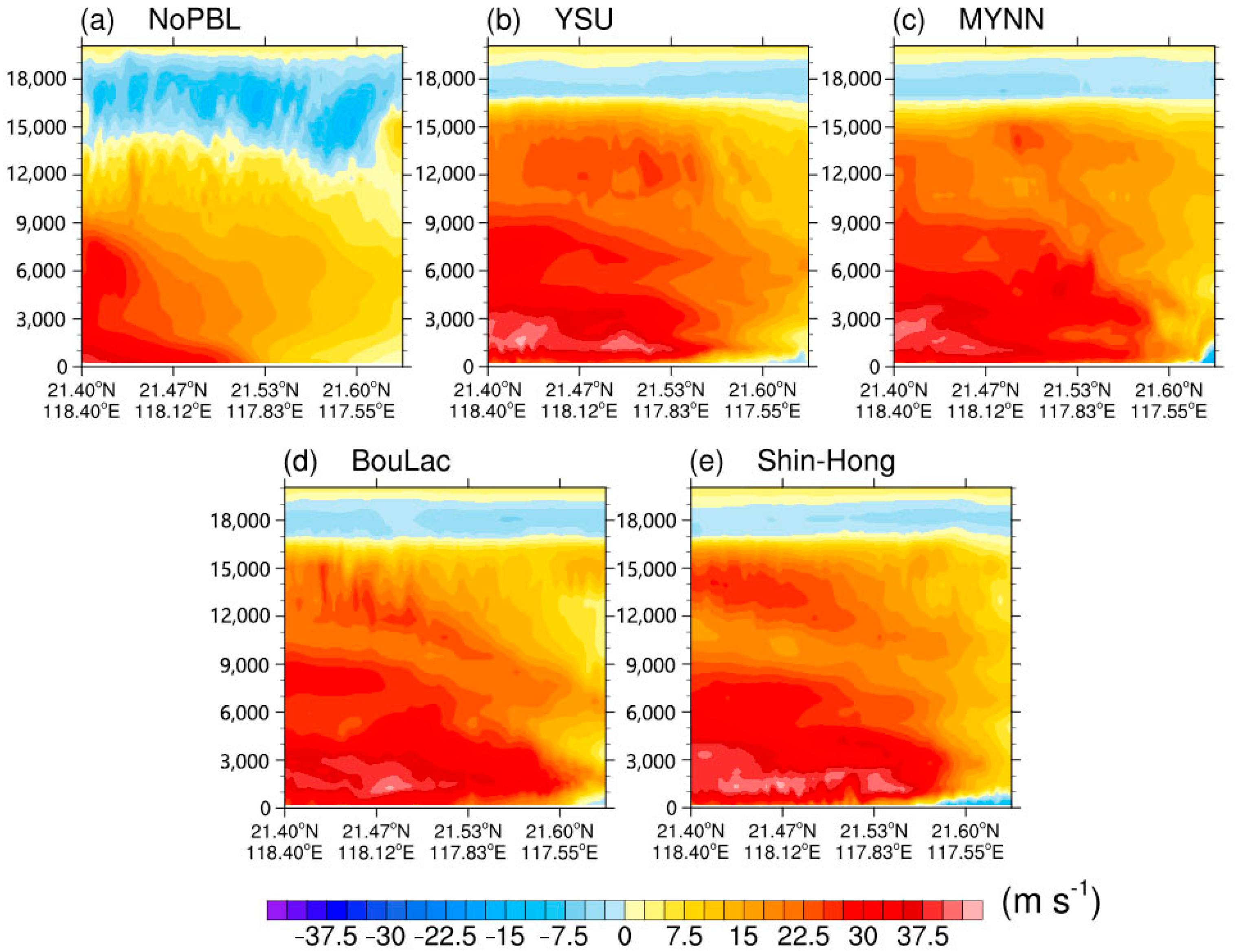
4.1. Characteristics of Simulated U-Wind

Compared with other boundary schemes, the U-wind simulations in the eye area of the YSU and MYNN schemes were more similar to the observation/result of an ideal typhoon model (shown in Figure 9). Here, the ideal typhoon model means the vertical typhoon structure analyzed in Emanuel et al. (1986) [26,27], Chen et al. (2019) [20], and Fei et al. (2021) [28], where the eye area sinks and both sides of the eye area rise. Under the action of guided wind circulation, the northeast to southwest of the U-wind boundary layer in the eye area showed an east-to-west wind transition, with an easterly jet near a height of 6000 m on the northeast side of the eye area and weak westerly winds on the southwest side of the upper levels. The YSU scheme (Figure 9b) simulated weak westerly and easterly winds at lower levels within the boundary layer, which were more consistent with the aircraft observations; the location of the easterly jet at the middle levels and weak westerly winds at the upper levels were more consistent with the ideal typhoon model. NoPBL (Figure 9a) simulated a weak variation in the wind speed intensity in the boundary layer; it could not simulate the easterly jet and weak westerly winds in the upper layers. The simulation results of the MYNN scheme (Figure 9c) were more like the YSU scheme, simulating weak westerly winds at the bottom and upper levels, as well as a strong easterly jet. The BouLac simulation scheme (Figure 9d) had a large area of westerly winds at the bottom, a low position for the westerly winds at the middle and upper positions, and a strong easterly jet. The Shin-Hong scheme (Figure 9e) simulated a small area of the bottom westerly wind and a strong upper westerly wind but incorrectly simulated the center of the westerly wind at the center of the typhoon eye.
In the U-wind simulation in the eyewall area (shown in Figure 10), the YSU and BouLac schemes were relatively close to the observation and ideal typhoon model. The U wind in the eyewall area was an easterly wind, with an easterly wind jet on the north side below a height of 9000 m and a weak westerly wind in the high-rise. NoPBL (Figure 10a) was weak; a high-rise weak westerly wind was not simulated. The YSU scheme (Figure 10b) could simulate the easterly wind jet below an altitude of 9000 m, which was more consistent with the aircraft observations. The middle-level easterly wind jet position and high-level weak westerly wind position were more consistent with the ideal typhoon model. The MYNN scheme (Figure 10c) was like the YSU scheme, but the easterly jet area was scattered under a height of 9000 m, which was inconsistent with the ideal model of the eyewall area, while the easterly jet area was weak. The BouLac scheme simulation (Figure 10d) had a large easterly wind area; the high-rise westerly wind speed was excessively strong. The Shin-Hong scheme (Figure 10e) simulated the easterly wind jet and strong high-rise weak westerly winds. Compared with the U-wind characteristics in the eye area, the easterly wind in the eyewall area was stronger than that in the eye area; the westerly wind in the eyewall area was significantly weaker than that in the eye area.

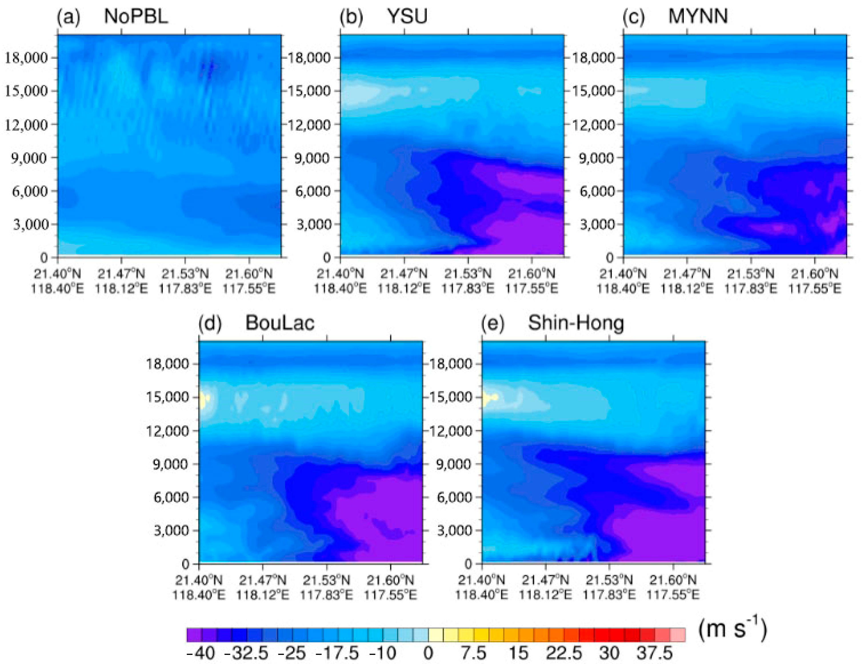
4.2. Characteristics of the Simulated V-Wind

In the V-wind simulation of the eye area (shown in Figure 11), the YSU scheme was more similar to the observation. The north–south wind transition was more notable on both sides of the eye area; there was a notable leftward dip at the north–south wind intersection from the lower to the upper levels. In the boundary layer, there was a north wind component in the jet on the southwestern side while there was a south wind rapid on the northeastern side. The southerly wind component was stronger than the northerly wind component under the action of the guiding wind; a weak northerly wind existed at the upper levels. The simulation results of the NoPBL (Figure 11a) were more like the mean values of the aircraft observation heights, but the entire spatial profile was weak for the V-wind speed simulations: the southern extension height was low and the jet within the boundary layer was not notable. The mean wind speed of the simulated V-wind in the YSU scheme (Figure 11b) deviated from the aircraft observation, but the intensity and location of the jet were more optimally simulated, with more pronounced characteristics in the high south wind extension height and a weak northerly wind in the upper levels. The simulation results of the MYNN scheme (Figure 11c) were similar to those of the YSU scheme, except that the MYNN scheme had an irregular south–north intersection and an elevated height for the strong southerly wind extension. The BouLac scheme (Figure 11d) was closer to the MYNN scheme, with differences in the shape of the north–south wind interface, as well as the strongest north–south wind jet in the boundary layer. The Shin-Hong scheme (Figure 11e) simulated a north–south wind interface similar to the YSU scheme, but the strength of the low-level north–south wind jet was the weakest among several parameterization schemes.
In the V wind simulation of the eyewall area (shown in Figure 12), the YSU scheme was similar to the observation. The middle and lower layers of the eyewall area were consistent with the southerly wind jet, with a southerly wind component in the boundary layer and a weak northerly wind component in the bottom and high layers. The NoPBL (Figure 12a) simulation results showed that the southerly wind component was too weak, the southerly wind component extension height was too low, and the thickness of the high-rise northerly wind was too thick. The YSU scheme (Figure 12b) could better simulate the strength and position of the southerly wind component jet current, as well as the thickness and strength of the high-rise north wind. The MYNN scheme (Figure 12c) was similar to the YSU scheme, but the southerly wind component jet surrounding area and shape were notably different. The BouLac scheme (Figure 12d) was close to the MYNN scheme; the jet position deviation in the southerly wind component was large. The Shin-Hong scheme (Figure 12e) strongly (excessively) simulated the southerly wind component area in the low layer and the northerly wind component in the low layer. Compared with the characteristics of the V-wind in the eye area, there was no north–south wind conversion interface in the eyewall area, while there was only the southerly wind jet flow and no northerly wind jet flow in the eyewall area.

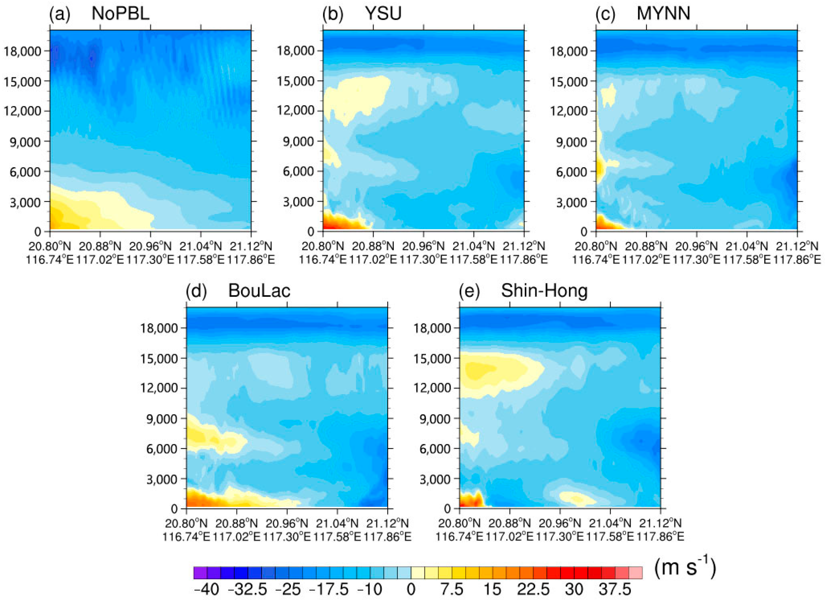
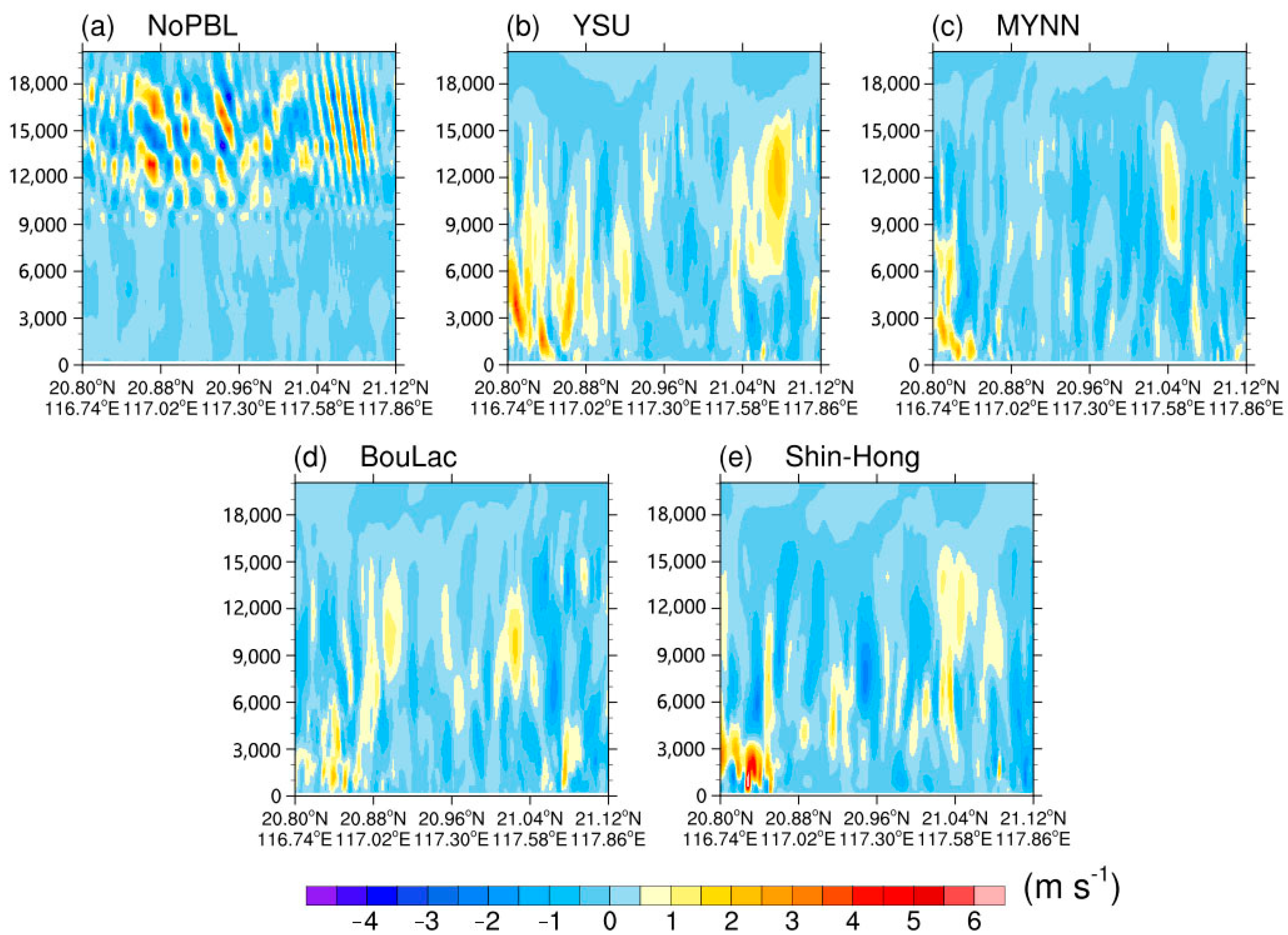
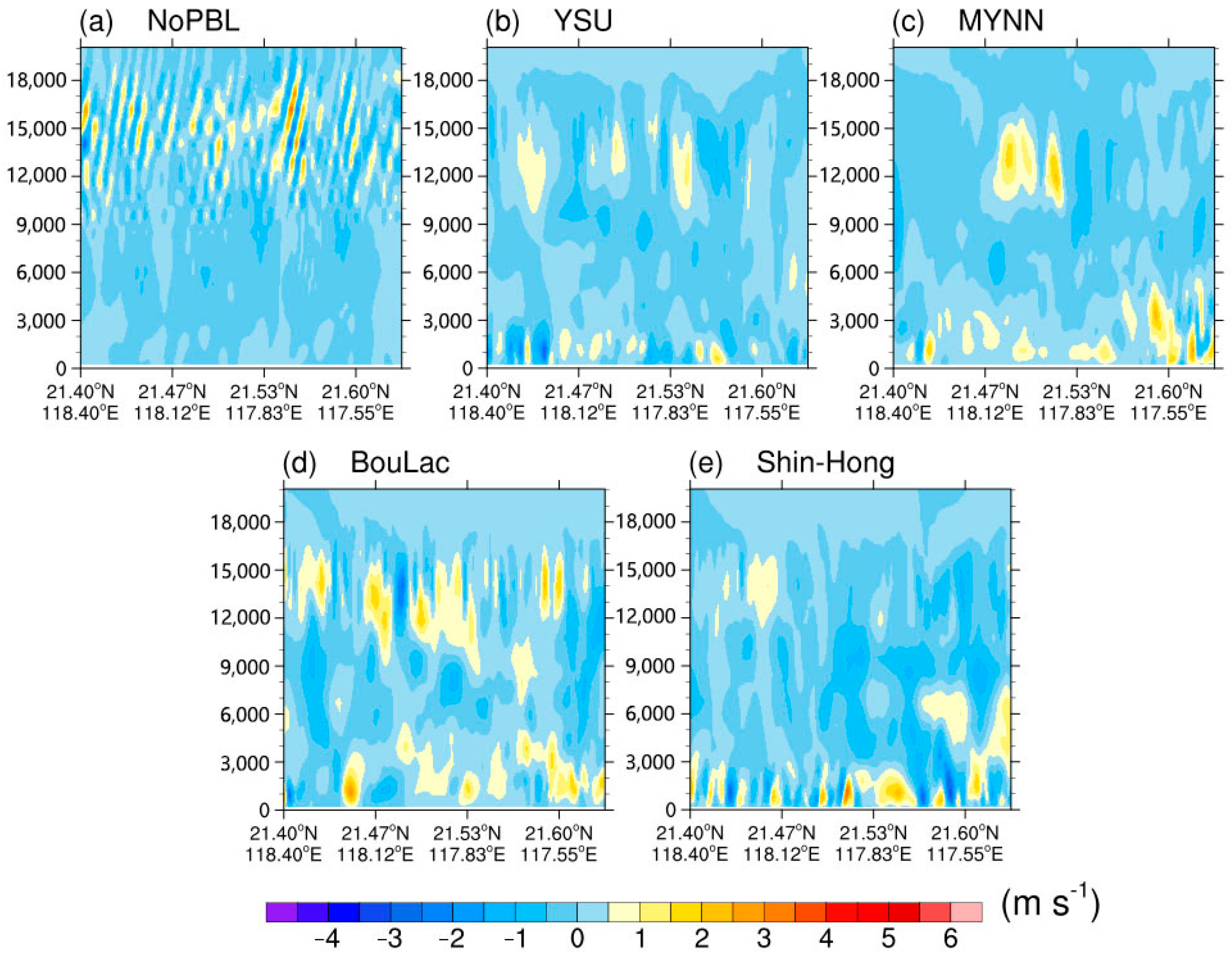
4.3. Characteristics of Simulated W-Wind

The MYNN and YSU schemes were similar to the observed and ideal models in the eye area W-wind simulation (Figure 13). In the eye of the typhoon, sinking motion was dominant. Ascending motion existed on both sides of the eye area; a lateral arrangement of the ascending and descending motion constituted the vertical circulation. NoPBL (Figure 13a) was poorly simulated, with mainly weak subsidence motion at the lower levels and the co-existence of the upward and downward motion at the upper levels. The YSU scheme (Figure 13b) could better simulate the characteristics of the eye area, which was closer to the ideal model and observations. The eye area mainly presented a sinking motion; the sides of the eye area were characterized by a strong rising motion. The MYNN scheme (Figure 13c) was similar to the YSU scheme, but the simulation of the intensity of the ascending motion on both sides of the eye center was weak, while the ascending motion on both sides of the eye area was asymmetrically distributed. The BouLac scheme (Figure 13d) poorly simulated the sinking movement area of the eye center. The sinking movement of the eye center position was strong. The upward movement on the left and right sides of the strong sinking movement was asymmetric. The Shin-Hong scheme (Figure 13e) substantially simulated the horizontal distribution of vertical movement. The upward movement on both sides of the eye center was asymmetric. Strong upward movement existed in the low layer along the southwest side.
In the wall W-wind simulation (Figure 14), the MYNN and YSU schemes were similar to the observation and ideal model. There was a coexistence between the upward movement and sinking motion in the eyewall area. The vertical movements of the low, middle, and high levels were strong. NoPBL (Figure 14a) had a poor simulation effect. The low layer was mainly characterized by a weak sinking motion; the high level was characterized by a rising and sinking motion, similar to the vertical motion simulated in the eye area. The YSU scheme (Figure 14b) could better simulate the characteristics of the eyewall area. The low layer of the eyewall area was mainly characterized by a rising motion. There was sinking motion on both sides of the upward movement, the characteristics of vertical circulation were notable, and the middle and high levels could better simulate the vertical circulation. The MYNN scheme (Figure 14c) could better simulate the rising motion of the lower level, while the lower layer sinking motion simulation was poor; the middle and high levels could only simulate the local vertical circulation. Strong upward and downward motions were simulated by the BouLac scheme (Figure 14d). The Shin-Hong scheme (Figure 14e) showed that the simulated low-layer vertical motion was strong; the simulated middle- and high-level sinking motion was strong. Compared with the W-wind characteristics of the eye area, there was no unique sinking area within the eyewall area. The rising and sinking movements of the lower layer were evenly distributed. The overall vertical movement was weaker than that of the eye area.

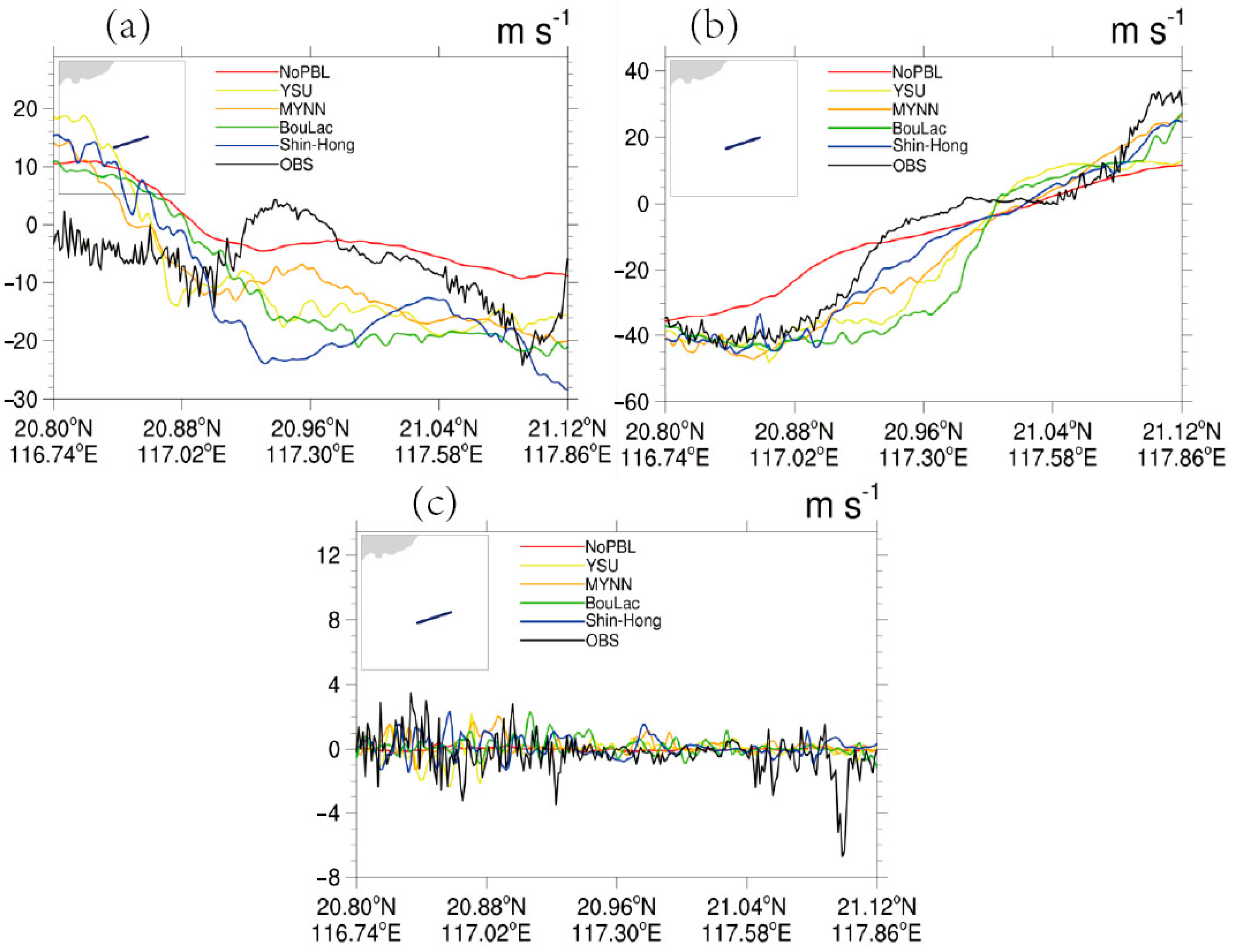
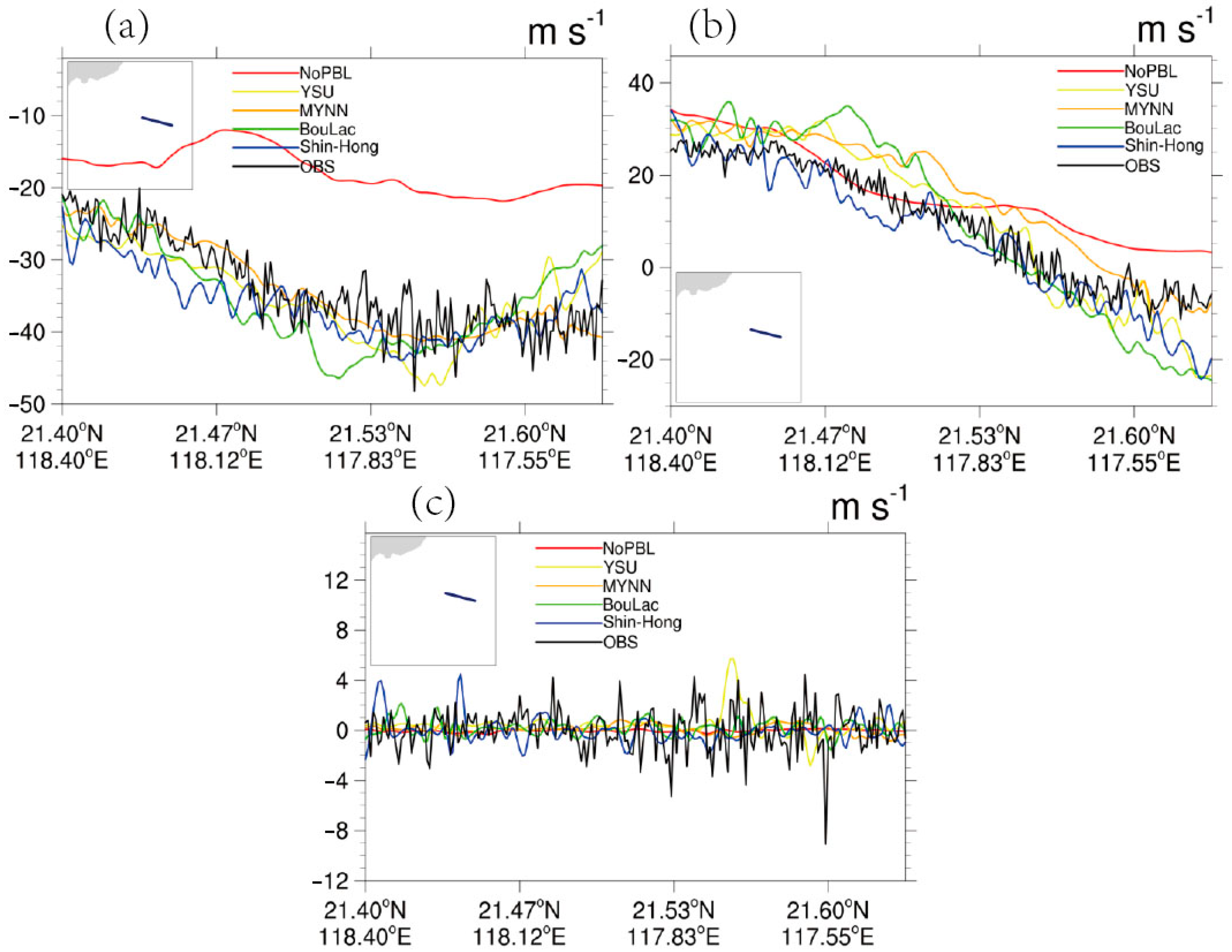
4.4. Comparison of the Winds with Aircraft Observations

Based on Table 3, there were notable wind speed differences between areas II and IV. The U- and V-winds in the eyewall zone were notably larger than those in the eyewall zone. The vertical motion in the eyewall zone was notably larger than that in the eyewall zone. There were deviations in the simulation of vertical motion using each parameterization scheme. Based on our comprehensive analysis, better simulations in areas II (Figure 15) and IV (Figure 16) were obtained from the MYNN and YSU schemes. The YSU scheme especially was closer overall to the ideal model and boundary layer observation.

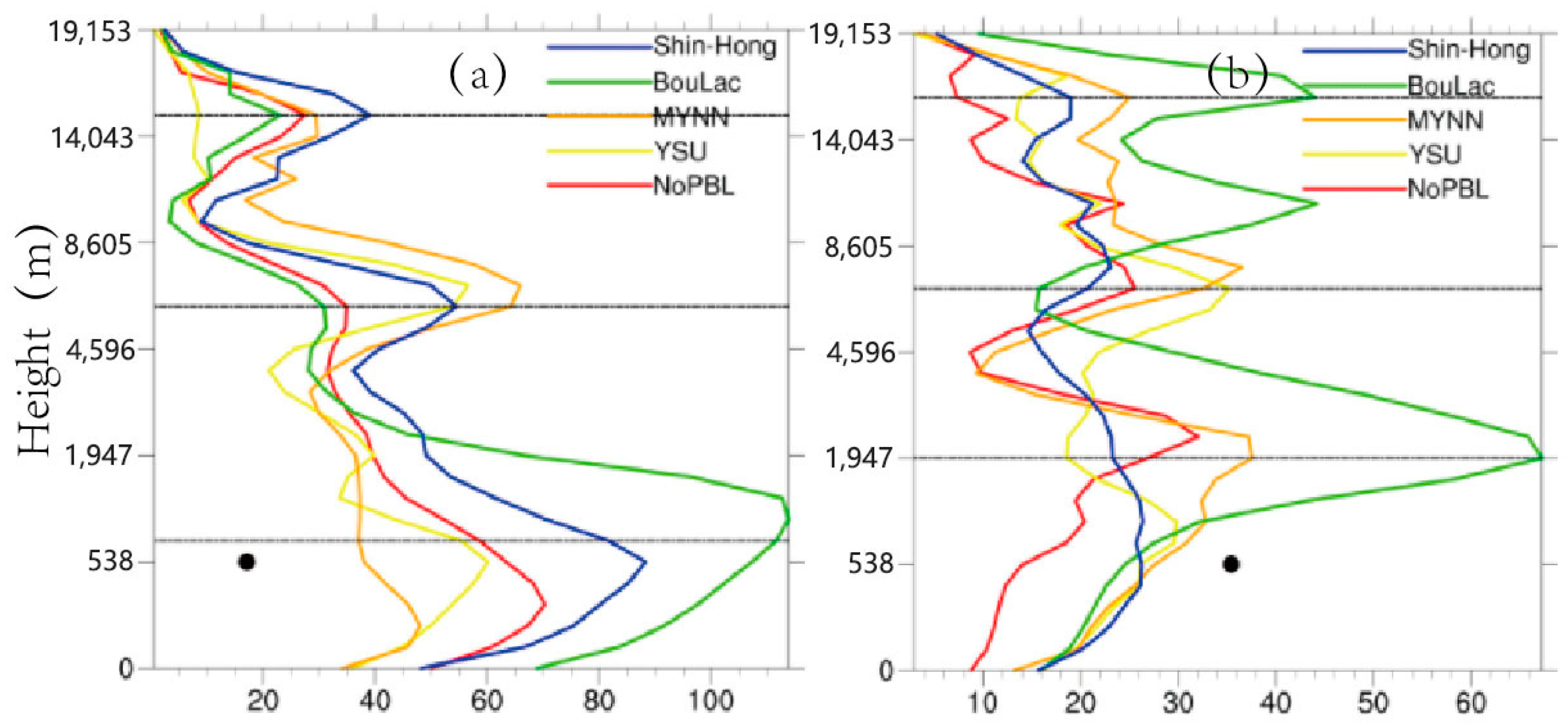
4.5. Turbulent Kinetic Energy

According to the simulation results of TKE throughout the entire layer (Figure 17), there were three high-value regions of turbulent kinetic energy in the eye region (Figure 17a) and eyewall region (Figure 17b). Here, the average value was a spatial average, which was consistent with the aircraft observation path for easy comparative analysis. The trend in the simulation results in the eye region was more consistent than that in the eyewall region for several schemes. From the eye region simulation, the BouLac scheme had a higher turbulent kinetic energy in the lower layer simulation and a lower turbulent intensity in the higher layer simulation. The MYNN scheme was opposite to the BouLac scheme, with NoPBL located in the center position and the YSU and MYNN schemes having the lowest TKE. The TKE in the boundary layer was evidently higher in the simulations of several schemes than that from the aircraft observations (black dot in Figure 17a), whereas the MYNN and YSU schemes were closer to these observations. From the simulation of the eyewall region, the BouLac scheme had a higher TKE in the entire simulation, while the NoPBL simulation had the lowest TKE. The YSU and MYNN schemes had similar TKEs, which were also similar to those in the aircraft observations (black dot in Figure 17b). The TKE in the boundary layer was evidently lower in the simulations of several schemes than in the aircraft observations.

5. Conclusions and Discussions

Typhoon Nida passed through the Philippines and became a strong typhoon in the South China Sea; it then made landfall in Shenzhen, China. Based on the GPM satellite, observations revealed its reduced precipitation structure in the south. The boundary layer parameterization scheme had a key impact on the core simulation of the typhoon. The simulation results of several parameterization schemes show the following:
(1)
In the eye area, the simulation results of the YSU and MYNN schemes were relatively close to those of aircraft observations and the ideal typhoon model. In the V-wind simulation, the YSU scheme was similar to the observation. The interface of the north–south wind had a clear leftward inclination from low to high levels. The W-wind MYNN and YSU schemes were similar to the observation and ideal model. The eye center was mainly characterized by sinking movement. There was upward movement on both sides of the eye area, as well as upward and sinking movements that formed vertical circulation.
(2)
The U-wind YSU and BouLac schemes in the eyewall area were similar to the observation and ideal typhoon model. The V-wind of the YSU scheme was similar to the observation; the southerly wind component jet existed in the boundary layer. The W-wind MYNN and YSU schemes were similar to the observation and ideal model. Rising and sinking movements coexisted; vertical motion in the low layer and middle and high levels was strong.
(3)
Compared with the eye area, the U-wind in the eyewall area was strong. The V-wind did not have a conversion interface for the north and south wind. The W-wind had no unique whole-layer sinking area. The rising and sinking movements of the lower layer were evenly distributed, with weak overall vertical movement.
(4)
The YSU and MYNN schemes had similar TKEs, which were similar to those in the aircraft observations, but those in the simulations of several schemes in the boundary layer were evidently lower.
There was a notable difference in wind speed in the eye area and the eyewall area. The U-wind and V-wind in the eyewall area were significantly larger than those in the eye area; vertical movement in the eye area was significantly larger than that in the eyewall area. Each parameterization scheme deviated from the vertical movement simulation. According to our comprehensive analysis, the MYNN and YSU schemes were optimal. The YSU scheme was especially similar overall to the ideal model and boundary layer observation. The South China Sea is an important area for the generation and development of tropical cyclones. Therefore, we must refine the path, intensity, and spatial structure of generated and developing tropical cyclones. The aircraft observation data could verify the mode simulation capability and improve it accordingly. To examine the parameterization effects of numerical simulations of the typhoon boundary layer more effectively in the South China Sea, future studies should provide more simulation and analysis examples. In the present study, the aircraft observations obtained in Cartesian coordinates were used to analyze and discuss the simulation. Bao et al. (2020, 2022) [29,30] discussed the results of Hurricane Weather Research and Forecast system numerical simulation in a cylindrical polar coordinate framework. This can directly examine the critical radially inflowing and tangential winds. To further study the typhoon of the critical radially inflowing, tangential winds, and the mean wind profiles, we will convert the observations to cylindrical polar coordinates for enhanced analysis in the future.

Author Contributions

Conceptualization, M.Z. and W.L.; methodology, Z.Z. and M.Z.; formal analysis, C.T., M.X., and C.N.; writing—original draft preparation, C.T.; writing—review and editing, S.C. and C.T. All authors have read and agreed to the published version of the manuscript.

Funding

This research was funded by the Guangdong Major Project of Basic and Applied Basic Research (grant no. 2020B0301030004), Innovation Group Project of Southern Marine Science and Engineering Guangdong Laboratory (Zhuhai) (grant no. 311022006), China Meteorological Administration Innovation Development Project (grant no. 23202004045), Scientific Research Plan Project of Guangxi Meteorological Bureau (grant no. 2023ZL04), Laboratory of Beihai National Climate Observatory (grant no. BNCO-N202302), Guangdong Basic and Applied Basic Research Foundation (grant no. 2022A1515011100 and 2020A1515011034), and National Natural Science Foundation of China (grant nos. 42275002 and 42075004).

Informed Consent Statement

Not applicable.

Data Availability Statement

IMERG products provide precipitation data available through NASA (http://pmm.nasa.gov/data-access/downloads/gpm, accessed on 31 August 2023). The TC best-track dataset related to this article can be found at http://tcdata.typhoon.org.cn/, which is hosted by the Shanghai Typhoon Institute of the China Meteorological Administration [21]. ERA5 reanalysis data is available from the ECWMF (https://cds.climate.copernicus.eu/cdsapp#!/dataset/reanalysis-era5-single-levels?tab=form, accessed on 31 August 2023). NCEP-FNL is available from http://rda.ucar.edu/datasets/ds083.2, accessed on 31 August 2023.

Conflicts of Interest

The authors declare no conflict of interest. The funders had no role in the design of the study; in the collection, analyses, or interpretation of data; in the writing of the manuscript; or in the decision to publish the results.

References

  1. Tan, Z.-M.; Lei, L.; Wang, Y.; Xu, Y.; Zhang, Y. Typhoon Track, Intensity, and Structure: From Theory to Prediction. Adv. Atmos. Sci. 2022, 39, 1789–1799. [Google Scholar] [CrossRef]
  2. Hong, S.-Y.; Noh, Y.; Dudhia, J. A New Vertical Diffusion Package with an Explicit Treatment of Entrainment Processes. Mon. Weather. Rev. 2006, 134, 2318–2341. [Google Scholar] [CrossRef]
  3. Troen, I.B.; Mahrt, L. A simple model of the atmospheric boundary layer; sensitivity to surface evaporation. Bound.-Layer Meteorol. 1986, 37, 129–148. [Google Scholar] [CrossRef]
  4. Hong, S.Y.; Pan, H.L. Nonlocal boundary layer vertical diffusion in a Medium-Range Forecast Model. Mon. Weather Rev. 1996, 124, 2322–2339. [Google Scholar] [CrossRef]
  5. Nakanishi, M.; Niino, H. An Improved Mellor-Yamada Level-3 Model: Its Numerical Stability and Application to a Regional Prediction of Advection Fog. Bound.-Layer Meteorol. 2006, 119, 397–407. [Google Scholar] [CrossRef]
  6. Nakanishi, M.; Niino, H. Development of an Improved Turbulence Closure Model for the Atmospheric Boundary Layer. J. Meteorol. Soc. Jpn. Ser. II 2009, 87, 895–912. [Google Scholar] [CrossRef]
  7. Fitch, A.C.; Olson, J.B.; Lundquist, J.K.; Dudhia, J.; Gupta, A.K.; Michalakes, J.; Barstad, I.; Archer, C.L. Local and mesoscale impacts of wind farms as parameterized in a mesoscale NWP model. Mon. Wea. Rev. 2012, 140, 3017–3038. [Google Scholar] [CrossRef]
  8. Shin, H.H.; Hong, S.-Y. Representation of the Subgrid-Scale Turbulent Transport in Convective Boundary Layers at Gray-Zone Resolutions. Mon. Weather. Rev. 2015, 143, 250–271. [Google Scholar] [CrossRef]
  9. Nelson, M.A.; Conry, P.; Costigan, K.R.; Brown, M.J.; Meech, S.; Zajic, D.; Bieringer, P.E.; Annunzio, A.; Bieberbach, G. A Case Study of the Weather Research and Forecasting Model Applied to the Joint Urban 2003 Tracer Field Experiment. Part III: Boundary-Layer Parametrizations. Bound.-Layer Meteorol. 2022, 183, 381–405. [Google Scholar] [CrossRef]
  10. Pradhan, P.K.; Liberato, M.L.R.; Kumar, V.; Rao, S.V.B.; Ferreira, J.; Sinha, T. Simulation of mid-latitude winter storms over the North Atlantic Ocean: Impact of boundary layer parameterization schemes. Clim. Dyn. 2019, 53, 6785–6814. [Google Scholar] [CrossRef]
  11. Pradhan, P.; Liberato, M.L.; Ferreira, J.A.; Dasamsetti, S.; Rao, S.V.B. Characteristics of different convective parameterization schemes on the simulation of intensity and track of severe extratropical cyclones over North Atlantic. Atmos. Res. 2018, 199, 128–144. [Google Scholar] [CrossRef]
  12. Shen, Y.; Du, Y. Sensitivity of boundary layer parameterization schemes in a marine boundary layer jet and associated precipitation during a coastal warm-sector heavy rainfall event. Front. Earth Sci. 2023, 10, 1085136. [Google Scholar] [CrossRef]
  13. Fang, G.H.; Susanto, D.; Soesilo, I.; Zheng, Q.A.; Qiao, F.L.; Wei, Z.X. A note on the South China Sea shallow interocean circulation. Adv. Atmos. Sci. 2005, 22, 946–954. [Google Scholar] [CrossRef]
  14. Zhao, Z.; Chan, P.W.; Wu, N.; Zhang, J.A.; Hon, K.K. Aircraft Observations of Turbulence Characteristics in the Tropical Cyclone Boundary Layer. Bound.-Layer Meteorol. 2019, 174, 493–511. [Google Scholar] [CrossRef]
  15. Tang, J.; Zhang, J.A.; Chan, P.; Hon, K.; Lei, X.; Wang, Y. A direct aircraft observation of helical rolls in the tropical cyclone boundary layer. Sci. Rep. 2021, 11, 18771. [Google Scholar] [CrossRef]
  16. Alam, M. Sensitivity Study of Planetary Boundary Layer Parameterization Schemes for the Simulation of Tropical Cyclone ‘Fani’ Over the Bay of Bengal Using High Resolution Wrf-Arw Model. J. Eng. Sci. 2020, 11, 1–18. [Google Scholar] [CrossRef]
  17. Beswick, K.M.; Gallagher, M.W.; Webb, A.R.; Norton, E.G.; Perry, F. Application of the Aventech AIMMS20AQ airborne probe for turbulence measurements during the Convective Storm Initiation Project. Atmos. Meas. Tech. 2008, 8, 5449–5463. [Google Scholar] [CrossRef]
  18. Foster, S.; Chan, P.W. Improving the wind and temperature measurements of an airborne meteorological measuring system. J. Zhejiang Univ. A 2012, 13, 723–746. [Google Scholar] [CrossRef]
  19. Sun, W.; Sun, Y.; Zhang, Y.; Qiu, Q.; Wang, T.; Wang, Y. Ground validation of GPM IMERG rainfall products over the Capital Circle in Northeast China on rainstorm monitoring. In Proceedings of the Remote Sensing for Agriculture, Ecosystems, and Hydrology XX, Berlin, Germany, 10–13 September 2018; Volume 10783, p. 107831S. [Google Scholar] [CrossRef]
  20. Chen, Y.; Zhang, A.; Zhang, Y.; Cui, C.; Wan, R.; Wang, B.; Fu, Y. A Heavy Precipitation Event in the Yangtze River Basin Led by an Eastward Moving Tibetan Plateau Cloud System in the Summer of 2016. J. Geophys. Res. Atmos. 2020, 125, e2020JD032429. [Google Scholar] [CrossRef]
  21. Ying, M.; Zhang, W.; Yu, H.; Lu, X.; Feng, J.; Fan, Y.; Zhu, Y.; Chen, D. An Overview of the China Meteorological Administration Tropical Cyclone Database. J. Atmos. Ocean. Technol. 2014, 31, 287–301. [Google Scholar] [CrossRef]
  22. Zhang, H.S. Fundamentals of Atmospheric Turbulence; Peking University Press: Beijing, China, 2014. [Google Scholar]
  23. Mahala, B.K.; Mohanty, P.K.; Nayak, B.K. Impact of Microphysics Schemes in the Simulation of Cyclone Phailinusing WRF Model. Procedia Eng. 2015, 116, 655–662. [Google Scholar] [CrossRef]
  24. Skamarock, W.C.; Klemp, J.B.; Dudhia, J.; Gill, D.O.; Liu, Z.; Berner, J.; Wang, W.; Powers, J.G.; Duda, M.G.; Barker, D.M.; et al. A Description of the Advanced Research WRF, Version 4; National Center for Atmospheric Research: Boulder, CO, USA, 2019. [Google Scholar]
  25. Fang, R.; Chen, S.; Zhou, M.; Li, W.; Xiao, H.; Zhan, T.; Wu, Y.; Liu, H.; Tu, C. Periodic Cycles of Eyewall Convection Limit the Rapid Intensification of Typhoon Hato (2017). Adv. Meteorol. 2021, 2021, 5557448. [Google Scholar] [CrossRef]
  26. Emanuel, K.A. An air-sea interaction theory for tropical cyclones. Part I, Steady state maintenance. J. Atmos. Sci. 1986, 43, 585–605. [Google Scholar] [CrossRef]
  27. Chen, S.; Li, W.; Wen, Z.; Lu, Y.; Zhou, M.; Qian, Y.; Chen, G. Vertical Motions Prior to the Intensification of Simulated Typhoon Hagupit (2008). J. Geophys. Res. Oceans 2019, 124, 577–592. [Google Scholar] [CrossRef]
  28. Fei, R.; Wang, Y.; Li, Y. Contribution of Vertical Advection to Supergradient Wind in Tropical Cyclone Boundary Layer: A Numerical Study. J. Atmos. Sci. 2021, 78, 1057–1073. [Google Scholar] [CrossRef]
  29. Bao, S.; Bernardet, L.; Thompson, G.; Kalina, E.; Newman, K.; Biswas, M.; Shaowu, B. Impact of the Hydrometeor Vertical Advection Method on HWRF’s Simulated Hurricane Structure. Weather. Forecast. 2020, 35, 723–737. [Google Scholar] [CrossRef]
  30. Bao, S.; Zhang, Z.; Kalina, E.; Liu, B. The Use of Composite GOES-R Satellite Imagery to Evaluate a TC Intensity and Vortex Structure Forecast by an FV3GFS-Based Hurricane Forecast Model. Atmosphere 2022, 13, 126. [Google Scholar] [CrossRef]
Figure 1. Typhoon track, aircraft track, and typhoon precipitation distribution. Here, the fine solid line is the typhoon track; the coarse solid line is the flight track; shading shows the precipitation (unit: mm h−1); the yellow arrow indicates the flight track; the black arrow indicates the typhoon path; (a) the color map of satellite observation precipitation 7:30 to 7:59 on 1 August 2016; (b) the color map of IMERG satellite observation precipitation 8:00 to 8:30 on 1 August 2016.
Atmosphere 14 01403 g001
Figure 2. The observational track of Typhoon Nida at 6 h intervals from CMA best track data, the simulation period (time in blue color), and domain configuration for the numerical simulations.
Atmosphere 14 01403 g002
Figure 3. The radius of TC’s maximum wind in different experiments simulated at (a) sea level and (b) 6.0 km over time.
Atmosphere 14 01403 g003
Figure 4. (a) Schematic diagram for the analysis of Typhoon Nida: shading is the IMERG satellite observation precipitation 8:00 to 8:30, 1 August 2016 (unit: mm h−1). Red box indicates the weak eyewall area on the north side (area I; analysis period: 7:30–7:50), blue box indicates the eye area (area II; analysis period: 7:50–8:10), black box indicates the deep convection area on the south side (area III; analysis period: 8:10–8:30), and yellow box indicates the weak eyewall area on the west (area IV; analysis period: 8:30–8:55). (b) Sea level pressure (contours; unit: hPa) and 10 m winds (vector; m s−1) at 8:00, 1 August 2016, from ERA5 data.
Atmosphere 14 01403 g004
Figure 5. Track of typhoon Nida simulated using different parameterization schemes in domain 2.
Atmosphere 14 01403 g005
Figure 6. Plot of (a) track errors and (b) pressure differences with time in domain 2.
Atmosphere 14 01403 g006
Figure 7. Maximum wind speed of Typhoon Nida simulated using each parameterization scheme in domain 2 at a height of 10 m.
Atmosphere 14 01403 g007
Figure 8. Simulated precipitations (mm) using different parameterization schemes: (a) NoPBL scheme, (b) YSU scheme, (c) MYNN scheme, (d) BouLac scheme, (e) Shin-Hong scheme, and (f) observations from GPM data.
Atmosphere 14 01403 g008
Figure 9. Vertical cross-section of the U component of velocity in area II: (a) NoPBL scheme, (b) YSU scheme, (c) MYNN scheme, (d) BouLac scheme, and (e) Shin-Hong scheme.
Atmosphere 14 01403 g009
Figure 10. Vertical cross-section of the U component of velocity in area IV: (a) NoPBL scheme, (b) YSU scheme, (c) MYNN scheme, (d) BouLac scheme, and (e) Shin-Hong scheme.
Atmosphere 14 01403 g010
Figure 11. Vertical cross-section of the V component of velocity in area II: (a) NoPBL scheme, (b) YSU scheme, (c) MYNN scheme, (d) BouLac scheme, and (e) Shin-Hong scheme.
Atmosphere 14 01403 g011
Figure 12. Vertical cross-section of the V component of velocity in area IV: (a) NoPBL scheme, (b) YSU scheme, (c) MYNN scheme, (d) BouLac scheme, and (e) Shin-Hong scheme.
Atmosphere 14 01403 g012
Figure 13. Vertical cross-section of the W component of velocity in area II: (a) NoPBL scheme, (b) YSU scheme, (c) MYNN scheme, (d) BouLac scheme, and (e) Shin-Hong scheme.
Atmosphere 14 01403 g013
Figure 14. Vertical cross-section of the W component of velocity in area IV: (a) NoPBL scheme, (b) YSU scheme, (c) MYNN scheme, (d) BouLac scheme, and (e) Shin-Hong scheme.
Atmosphere 14 01403 g014
Figure 15. Comparison of simulated U/V/W with observation for area II: (a) U, (b) V, and (c) W.
Atmosphere 14 01403 g015
Figure 16. Comparison of simulated U/V/W with observation for area IV: (a) U, (b) V, and (c) W.
Atmosphere 14 01403 g016
Figure 17. Simulation results of the whole layer of the TKE: (a) area II and (b) area IV; black dots represent aircraft observation results.
Atmosphere 14 01403 g017
Table 1. Numerical experimental design of the boundary layer parameterization schemes.
Domain 1Domain 2Domain 3
Resolution4.5 km1.5 km0.5 km
Grid number598 × 4661237 × 643811 × 811
Microphysics schemesWSM 6-class graupel schemeWSM 6-class graupel schemeWSM 6-class graupel scheme
Cumulus schemesModified Tiedtke scheme (ARW only)No cumulusNo cumulus
Shortwave radiation schemesrrtmg schemerrtmg schemerrtmg scheme
Longwave radiation schemesrrtmg schemerrtmg schemerrtmg scheme
Land–surface schemeUnified Noah land–surface schemeUnified Noah land–surface schemeUnified Noah land–surface scheme
Table 2. The planetary boundary layer (PBL) scheme in the experiments.
Experiment NameDomain 1Domain 2Domain 3
NoPBLNo boundary-layer
YSUYSU scheme
MYNNMYNN 2.5 level TKE scheme
BouLacBougeault and Lacarrere PBL scheme
Shin-HongShin-Hong “scale-aware” PBL scheme
Table 3. Analysis of the spatial profile wind speed and boundary layer wind speed in areas II and IV.
AreaParameterization Scheme U ¯
(m s−1)
U ¯
(m s−1)
W ¯
(m s−1)
U S i m u a t e d U o b s e r v e d ¯ ¯
(m s−1)
V S i m u l a t e d V o b s e r v e d ¯ ¯
(m s−1)
W S i m u a t e d W o b s e r v e d ¯ ¯
(m s−1)
IINoPBL12.15.10.4214.47.40.787
YSU8.39.60.3887.68.90.729
MYNN9.68.10.3095.66.40.740
BouLac8.99.20.3368.010.10.755
Shin-Hong8.89.60.4099.55.00.665
IVNoPBL19.910.90.28716.24.21.227
YSU23.118.10.2433.75.31.038
MYNN23.217.80.2462.35.71.061
BouLac23.618.10.3644.67.51.005
Shin-Hong24.418.40.3533.74.41.105
Disclaimer/Publisher’s Note: The statements, opinions and data contained in all publications are solely those of the individual author(s) and contributor(s) and not of MDPI and/or the editor(s). MDPI and/or the editor(s) disclaim responsibility for any injury to people or property resulting from any ideas, methods, instructions or products referred to in the content.

