Article

Improving Risk Projection and Mapping of Coastal Flood Hazards Caused by Typhoon-Induced Storm Surges and Extreme Sea Levels

1
School of Economics and Management, North China Electric Power University, Beijing 102206, China
2
Department of Land Surveying and Geo-Informatics, The Hong Kong Polytechnic University, Hong Kong, China
3
Research Institute for Land and Space, The Hong Kong Polytechnic University, Hong Kong, China
4
Smart Cities Research Institute, The Hong Kong Polytechnic University, Hong Kong, China
*
Author to whom correspondence should be addressed.
Atmosphere 2023, 14(1), 52; https://doi.org/10.3390/atmos14010052
Submission received: 2 December 2022 / Revised: 21 December 2022 / Accepted: 23 December 2022 / Published: 27 December 2022
(This article belongs to the Special Issue Precipitation Observations and Prediction)

Abstract

:
Seawater inundation mapping plays a crucial role in climate change adaptation and flooding risk reduction for coastal low-lying areas. This study presents a new elevation model called the digital impermeable surface model (DISM) based on the topographical data acquired by unmanned aerial vehicle (UAVs) for improving seawater inundation mapping. The proposed DISM model, along with the bathtub model, was used to assess coastal vulnerability to flooding in significant tropical cyclone events in a low-lying region of Victoria Harbor in Hong Kong. The inundation simulations were evaluated based on the typhoon news and reports which indicated the actual storm surge flooding conditions. Our findings revealed that the proposed DISM obtains a higher accuracy than the existing digital elevation model (DEM) and the digital surface model (DSM) with a RMSE of 0.035 m. The DISM demonstrated a higher skill than the DEM and the DSM by better accounting for the water-repellent functionality of each geospatial feature and the water inflow under real-life conditions. The inundation simulations affirmed that at least 88.3% of the inundated areas could be recognized successfully in this newly-designed model. Our findings also revealed that accelerating sea level rise in Victoria Harbor may pose a flooding threat comparable to those induced by super typhoons by the end of the 21st century under two representative emission scenarios (RCP4.5 and RCP8.5). The seawater may overtop the existing protective measures and facilities, making it susceptible to flood-related hazards.

1. Introduction

Climate scientists have pointed out that global warming causes rising sea levels and the threats induced by extreme weather events are expected to be more severe [1,2]. In the past decades, severe typhoons frequently struck low-lying regions around the world, with concomitant storm surges causing intense seawater intrusion and inflicting substantial damage to coastal neighborhoods [3,4]. Estimating the vulnerability of coastal cities is paramount in formulating long-term adaptation measures and helping local communities understand and take necessary steps to alleviate emerging hazards [5].
To analyze how far the floodwater inundates, topographic data that represents the ground surface elevation is one of the primary inputs for hydraulic analysis [6,7]. The digital surface model (DSM) and the digital elevation model (DEM) are the prevalent elevation data used in previous flood modeling studies due to their accessibility and simplicity [8,9]. However, they have limitations which should be considered in flood analysis. Specifically, the DEM provides the bare ground’s elevation data and, therefore, tends to overestimate the inundation in an urban environment since the DEM has no surface objects (e.g., buildings, walls, road curbs and dykes) that could reduce the inland water flow [10]. Flood water commonly flows around buildings or other built-up land features instead of running through them, unless the water level rises above the crest height of the entrances of the first building floor [11,12]. In comparison, the DSM retains all the surface features, including natural and artificial objects (e.g., vegetation and bridges) regardless of the surface roughness and permeability [13]. Such a model tends to underestimate the total inundation area, especially when a constant Manning’s roughness value is used [14]. If the terrain surface model fails to take the permeability into account, it would be challenging to accurately simulate the actual landward flow of water and assess the flood vulnerability within the subject area [15]. Therefore, it is vital to create a topographic elevation model which is specified for the use of flood analysis for capturing and revealing the local flow dynamics under different flooding scenarios [6,16,17].
These digital geospatial models can be generated from many sources ranging from ground surveys to remotely sensed technology [18,19]. With the advancement of remote sensing technology, aerial photographs are widely adopted in the production of high-resolution and high-accuracy DEMs and DSMs [20]. Unmanned aerial vehicles (UAVs) are an emerging technology to measure and collect surface elevation data with higher efficiency and accuracy [21,22,23]. With a finer spatial resolution, the UAV-derived elevation model can substantially enhance the accuracy of the predicted flood inundation extent [24,25]. Meanwhile, most of the studies mainly focused on the quality and accuracy assessment of the drone-based DEM while the research about the means of accuracy improvement in a drone-related product was limited [26,27]. For this reason, it was necessary to explore the potential factors which can improve the accuracy of the outcomes and quantitatively identify the optimal UAV flight plan to capture the scenes and geometrical data in an urban setting [28,29].
Since climate change impacts are suggested to become more drastic and severe in the 21st century [30], seawater inundation risks are expected to intensify in a warming climate [31]. For example, under the high greenhouse gas emission scenario, the sea level in the vicinity of Hong Kong is expected to rise by 0.63 to 1.07 m by the end of this century (2081–2100) [32]. It is critical to examine whether the elevated sea level poses significant damage and destruction to the coastal low-lying areas through flood modeling, therefore facilitating policymakers to formulate a different strategy to protect the coastal communities from rising sea levels.
In this study, we will develop an improved photogrammetric model based on UAVs to conduct seawater inundation mapping during severe typhoon events in Hong Kong, which is the primary concern of Hong Kong’s Drainage Services Department and Civil Engineering and Development Department. Specifically, the optimal flight route design will be identified to construct photogrammetric models for the study area based on a wide variety of parameters (i.e., flight elevation, speed of the flight, image overlap and flight path). The constructed photogrammetric model will retain only the critical artificial structures that affect the seawater flow and will be termed the digital impermeable surface model (DISM) in this study. The accuracy of the proposed DISM model will be evaluated using visual inspection and performance metrics and compared to the DEM and the DSM. Seawater inundations maps will also be generated to visualize the flood-prone areas in different projected water level scenarios. The approach and findings of this study can also serve as a reference for coastal zones around the world.
The paper is organized as follows. Section 2 describes the models, datasets and performance metrics used in this study. Section 3 presents a thorough analysis and discussion on the evaluation of different models in simulating flood inundations and risk projection of coastal flood hazards under different scenarios of sea level rise. Finally, conclusions and findings of this study will be drawn in Section 4.

2. Methods and Data Sources
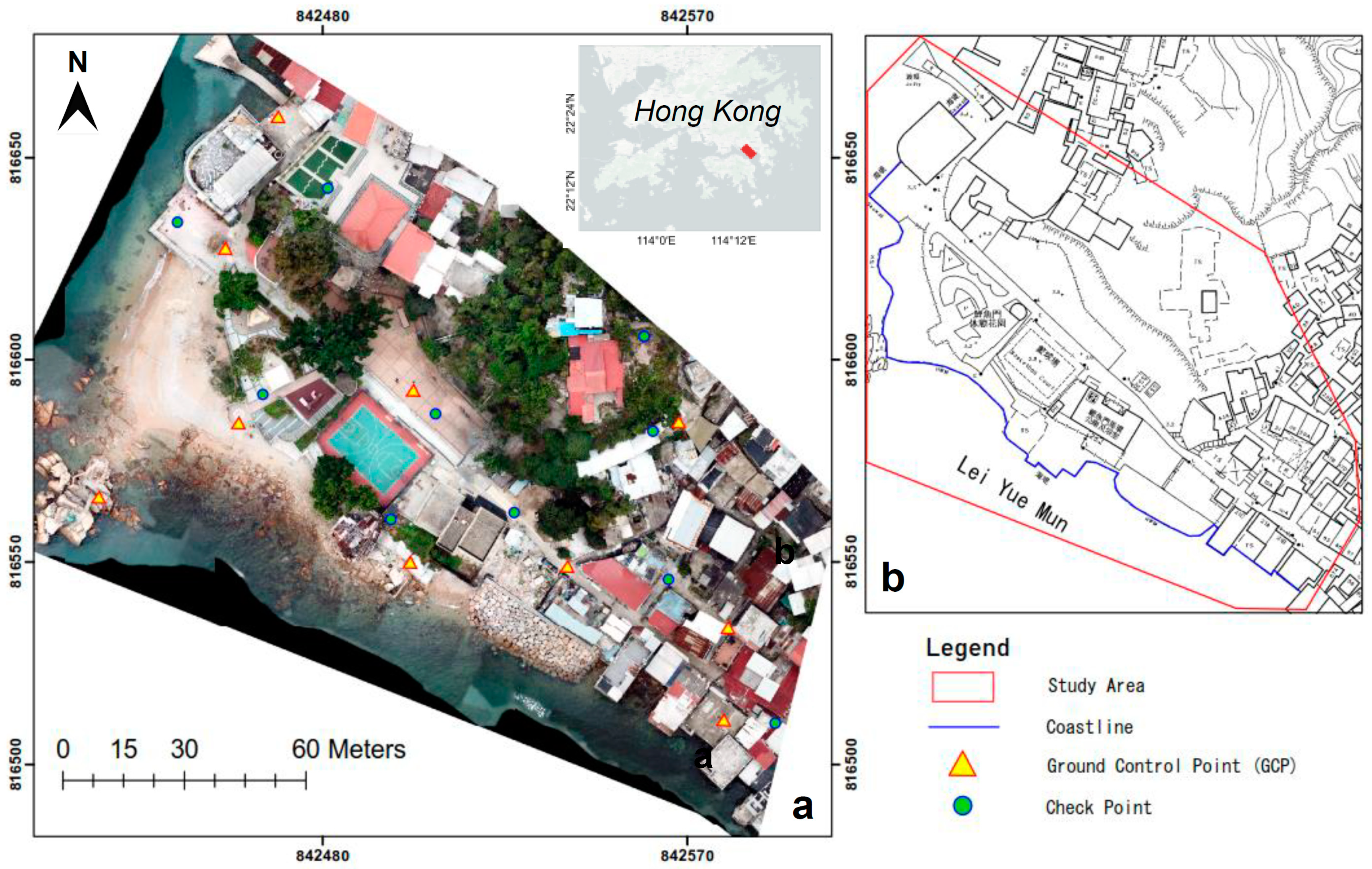
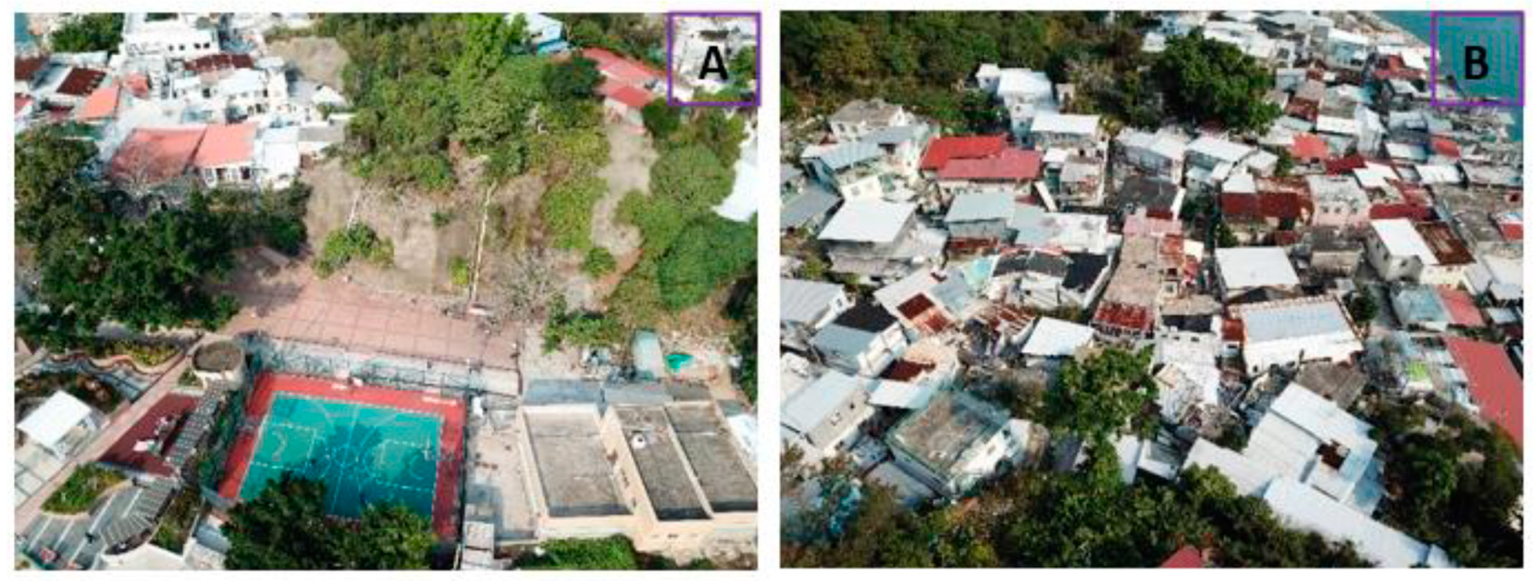
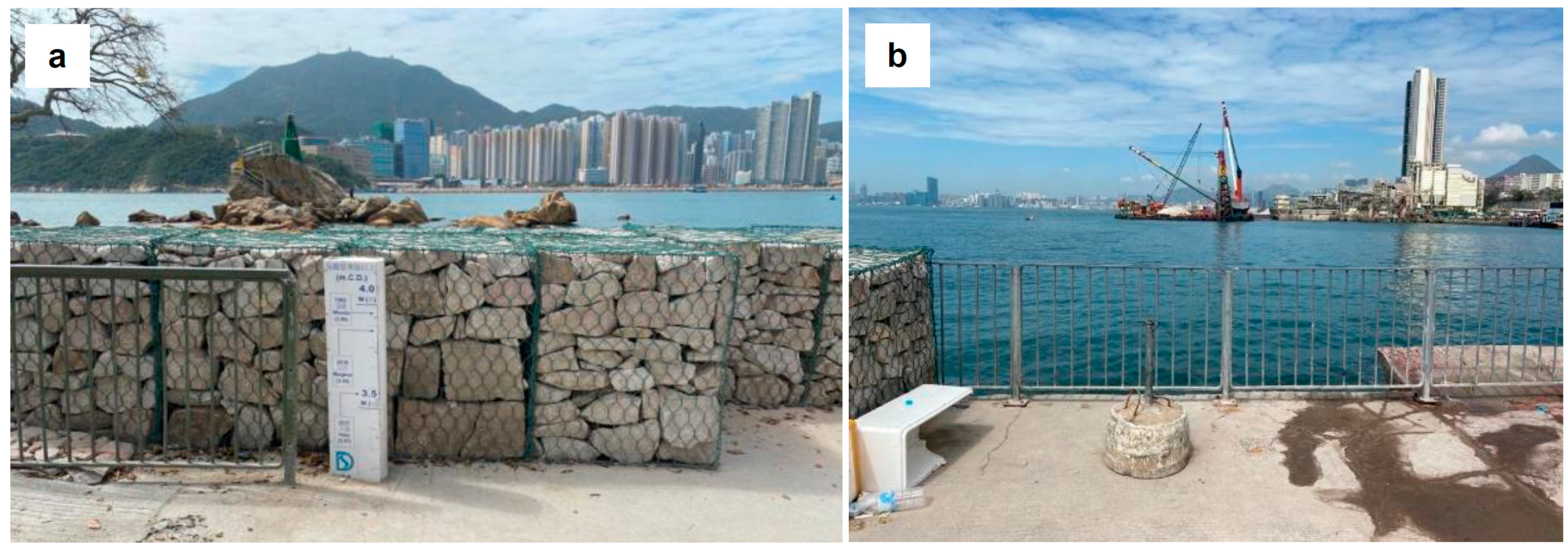
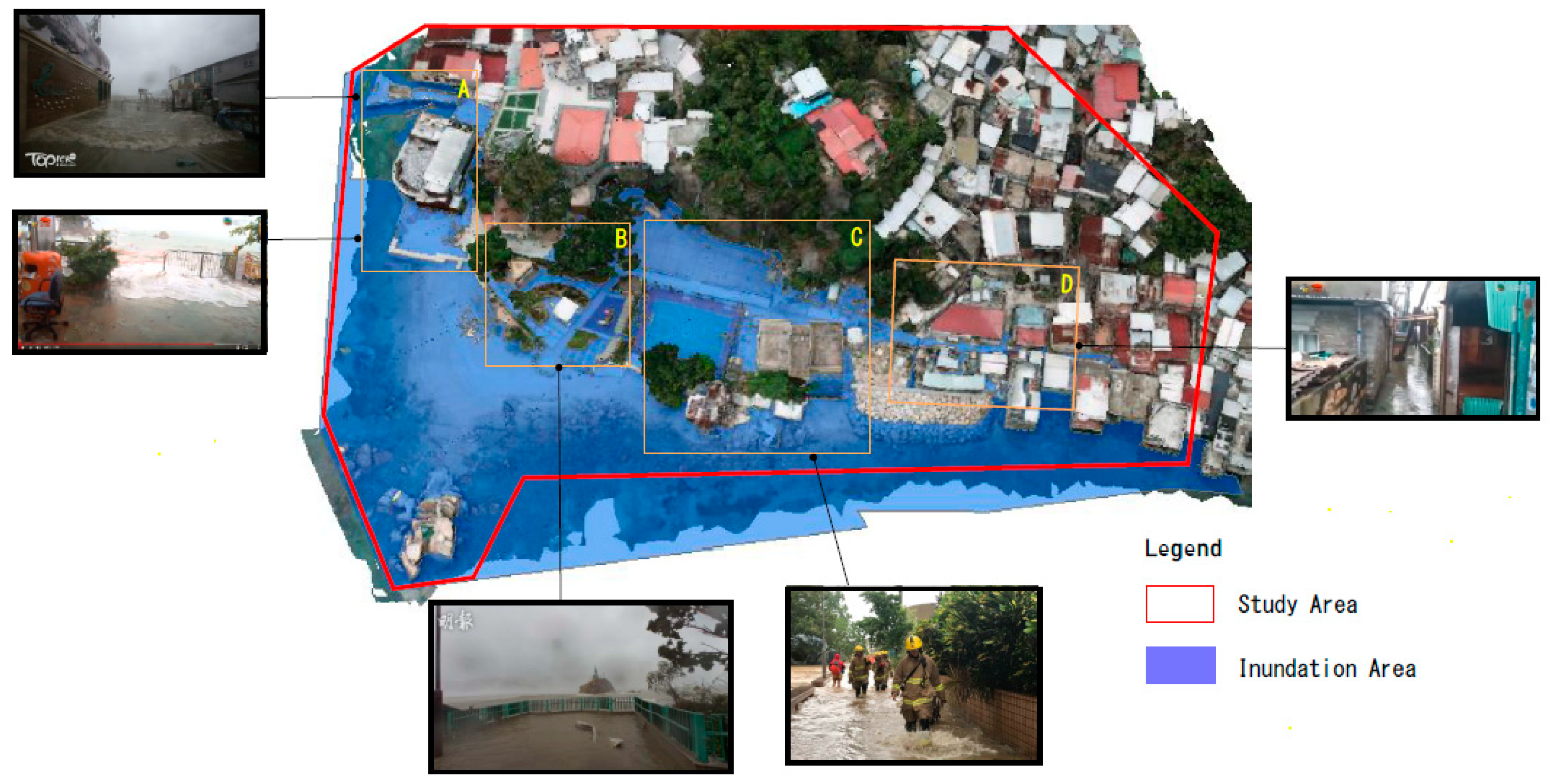
2.1. Study Area

The modeling area of this paper is located between the Sam Ka Tsuen and Ma Wan Village of Lei Yue Mun in Hong Kong, which covers approximately 32,634 m2 (Figure 1). This study area lies along the seafront of the eastern extent of Victoria Harbor and consists of residential and recreational areas. The media uncovered that the local Lei Yue Mun villagers who dwell in temporary housing are susceptible to severe seawater infusion during the onslaught of typhoons in Hong Kong. Therefore, it is suitable to act as an experimental site to analyze the storm surge hazard in the low-lying coastal area.

2.2. UAV Survey Planning

Four steps are required to develop the DISM, DSM and DEM. The first step was to acquire aerial images using a UAV. These images acted as a primary source of the terrain surface description in the study area. A multirotor drone, model DJI Mavic Pro PLATINUM, was used to perform all the flights for the data acquisition. This UAV was equipped with a 4000 × 3000 pixels CMOS camera sensor and supported manual control or automatic flying mode. The UAV was programmed to fly under the latter mode with double grid flight paths and an overlapping rate of 80% for the front and the side. Large overlaps were chosen in this study since smaller intersection angles will result in lower accuracy [33].
The second step was to become familiar with the site conditions and the environment, which was vital before flight planning. The elevation of the highest objects within the study area was identified. All the obstacles were recorded to set the thresholds of the flying altitude. Such a site inspection prevented the UAV from crashing into such objects when the flight mission was executed. In addition, accessible open space was required for take-off and landing during the site visit. For example, the areas shown in Figure 2B are not appropriate and safe landing sites.
The third step was to conduct the flight plan, which was achieved with the aid of an iOS application called Pix4Dcapture for the data acquisition. UAV flight planning involves the selection of flight modes, camera angles, image overlapping rates, drone speeds and flying altitudes. To evaluate the ideal imaging geometry and practical flight path for the production of an accurate photorealistic model and several elevation surface models, six different scenarios were tested (see Table 1). It included three main photogrammetric configuration datasets: only nadir images, only oblique images and both nadir and oblique images. Two flight modes were examined, including the double grid flight and circle plan. Generally, the double grid flight plan was suitable for both oblique and nadir images. Many researchers have confirmed it is optimal for mapping urban and built-up areas. On the other hand, the circular flight plan provided a circle around the study area. It is commonly adopted in mapping single buildings or other individual objects. It was still necessary to examine whether the images acquired by the circular flight plan could improve the reconstruction result and act as a supporting role to the double grid dataset in order to generate a photorealistic and accurate 3D mesh model of the complex urban area, similar to the study area. In terms of the camera angles, the nadir images are normally processed together with the oblique ones to strengthen the photogrammetric block [34]. Since there were various altitudes for the oblique images, it was quite demanding to assess which altitudes would be selected to incorporate with the nadir angles. Consequently, the high oblique images (close to the horizon) and the low oblique images were integrated separately with the vertical images to evaluate how the imaging angles influenced the accuracy and detail of the photogrammetric model output across the six scenarios. Since the differences between the camera angles in the same scenario did not exceed 45° [35], intermediate angles were used to link the nadir images and the oblique images. In addition, since UAV flight planning involves plenty of images overlapping with each other, an image overlapping rate of 80% was selected for both the settings of frontal and side overlaps to balance the efficiency and quality of the image acquisition. In terms of the drone speed, a low drone speed was adopted since a lower flying height required a lower drone speed to avoid blurred images [36]. However, a low drone speed would reduce the drone endurance and coverage of the study area to one battery load. Therefore, it was necessary to divide the low-flying height flight mission into two parts and resume the data collection after a battery change. For the UAV flying altitude, it was easy to obtain blurry images if the images were taken at a high altitude. The ground sampling distance (GSD) determined the spatial resolution. The higher the number of the image GSD, the poorer the spatial resolution and details of the image. It was, therefore, necessary to take the GSD into consideration when designing the flying height of each scenario. Two different flying heights were adopted and the GSDs of each scenario are presented in Table 1. Finally, the UAV with the six scenario settings was used to acquire images for further analysis.
The last step was to determine the distribution of the GCPs after the site reconnaissance. The GCPs are the critical element to obtain the georeference of a UAV photogrammetric block which can ensure aero-triangulation robustness. The GCPs were placed based on the following criteria: first, they must be visible from the sky and measured with survey equipment on the ground; second, the GCPs must be distributed well in the study area and at least three GCPs should be present in this study. Since previous studies have shown that 8–10 GCPs are sufficient to produce a reliable photogrammetric output [37], ten control points were measured with South GPS on site (see Figure 1a).

2.3. Data Collection

In this study, flight lines were conducted at different altitudes, ranging from 35 m to 55 m above the ground. The lowest altitude (35 m) was chosen so that the drone was close to the dwellings but at a sufficient distance from the tree crown that would guarantee safe flights without collisions. This lower altitude flight captured images with better details and higher spatial resolution which benefitted the visual interpretation. Conversely, the images taken at 55 m had a larger coverage of the study area which provided an overview of the entire work area and surroundings and reduced the flight duration [38].
Different camera angles such as 70°, 55°, 45°, 25° and 15° were employed in the multiple flight lines. The use of oblique images was particularly appropriate in rugged topography. If only the vertical images were utilized, many topographic details in the study area such as the façade of the small houses and fences of the playground may have been lost (see Figure 3a). However, it was hard to generate an orthophoto by solely using oblique images (Figure 3b). The combination of the nadir and oblique images prevented less void space in the resulting 3D model and enhanced the consistency of the reconstructed surfaces (Figure 3c).
The six scenarios of the UAV-derived images were processed to produce a set of point clouds with built-in parameters in Bentley’s ContextCapture software. The oblique and nadir images of all the flights were processed together in the ContextCapture Viewer. Ten GCPs were digitized and weighted equally in the photos in which they clearly appeared. This facilitated the software to fix the location of the control points, as well as the manual tie points which were used to enhance the reliability of the aero-triangulation and guide this process toward the correct photo positioning. The ContextCapture software started the aero-triangulation which included the self-calibrating bundle block adjustment (BBA) using both the internal orientation parameters of a camera (e.g., focal length, principal point and lens distortion items) and the external orientation parameters. This returned the quality report which listed the statistics about the model such as the calibration results, reprojection, control point and user tie point errors. When the statical report achieved a satisfactory result, the sparse point cloud model was ready to perform reconstruction and produce the dense point clouds and the 3D mesh model in a local Hong Kong 1980 Grid. Subsequently, the point clouds were filtered and segmented in accordance with the feature’s characteristics and permeability depending on which digital geospatial model was required. Finally, the point clouds were used to generate the DISM, DSM and DEM.

2.4. Seawater Inundation Simulation and Evaluation

The constructed DISM, DSM and DEM were used to develop the seawater inundation simulations in this study. The bathtub method, a classical method of flood mapping, was used to develop the inundation simulations during significant typhoon events, including Typhoon Mangkhut in 2018 [1], Typhoon Hato in 2017 [20], Typhoon Wipha in 2013 [25] and Typhoon Higos in 2020 [25]. The main idea of the bathtub method was to integrate extreme water levels with a digital elevation model to identify grid cells in the DEM that have a lower elevation than the projected water level in a flood event [6]. However, the conventional bathtub method does not account for surface connectivity, but we constructed the DSM, DEM and DISM with a 0.02 m spatial resolution for the data input of the bathtub method, which detected greater topographic complexity in the region of interest and fragmented the surface connectivity more easily. Therefore, the bathtub method used in this study identified the grid cells which fulfilled the two following requirements as inundation: (1) lower than the predicted water level and (2) connected to an adjacent flooded grid cell or open water.
Model validation is a key component of flood mapping as it concerns the evaluation of the model usability. Historical data from four major flood events that occurred in the vicinity of the study area were utilized for independent checking of the DISM. Generally, a comparison between the model results and the observed data are a common validation technique in flood hazard mapping. However, it depends solely on the availability of flood-related observation data. Apart from the maximum water depth information, no flow measurements were available from these events as no wireless sensor networks were found in the study area. Therefore, the simulated flood extents were assessed against the approximate value gathered from eyewitness accounts and historical photography across the study area since local TV news provided an overview of the flood-risk area and reported the flooding situation in local communities [39].

2.5. Evaluation Metrics

To test the performance of the six flight scenarios, two criteria were considered: first, quantitative analysis on the positional accuracy; second, a comparison based on the texture analysis. The model positional accuracy with respect to the 2D and 3D orientation was assessed according to Equations (1) and (2):
2 D   Error = ( d N ) 2 + ( d E ) 2
3 D   Error = ( d N ) 2 + ( d E ) 2 + ( d Z ) 2
where dN, dE and dZ are the residuals in northing, easting and height, respectively.
To compare the performance of the DISM, DSM and DEM, the vertical error of each model was evaluated through a comparison between the topographic data and 11 GPS-measured checkpoints taken at random positions within the study area. The quality of these models was assessed by the root mean square error (RMSE):
RMSE DISM , DSM , DEM = i = 1 n ( h GPS h DISM , DSM , DEM ) 2 n
where hGPS is the reference elevation (m) measured from GNSS-RTK, hDISM,DSM,DEM is the corresponding value derived from each model and n corresponds to the total number of checkpoints.

3. Results and Discussions

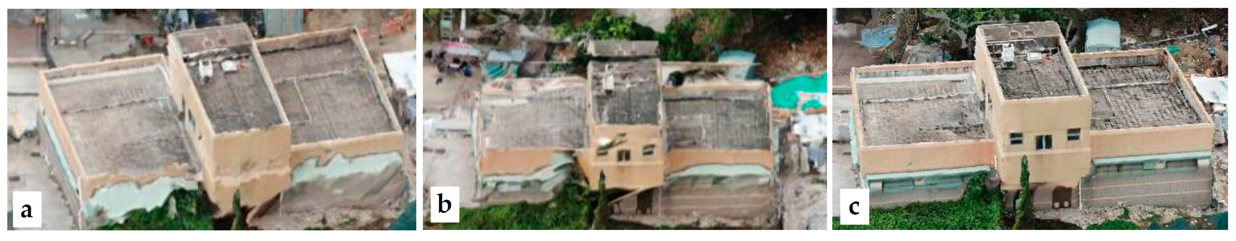
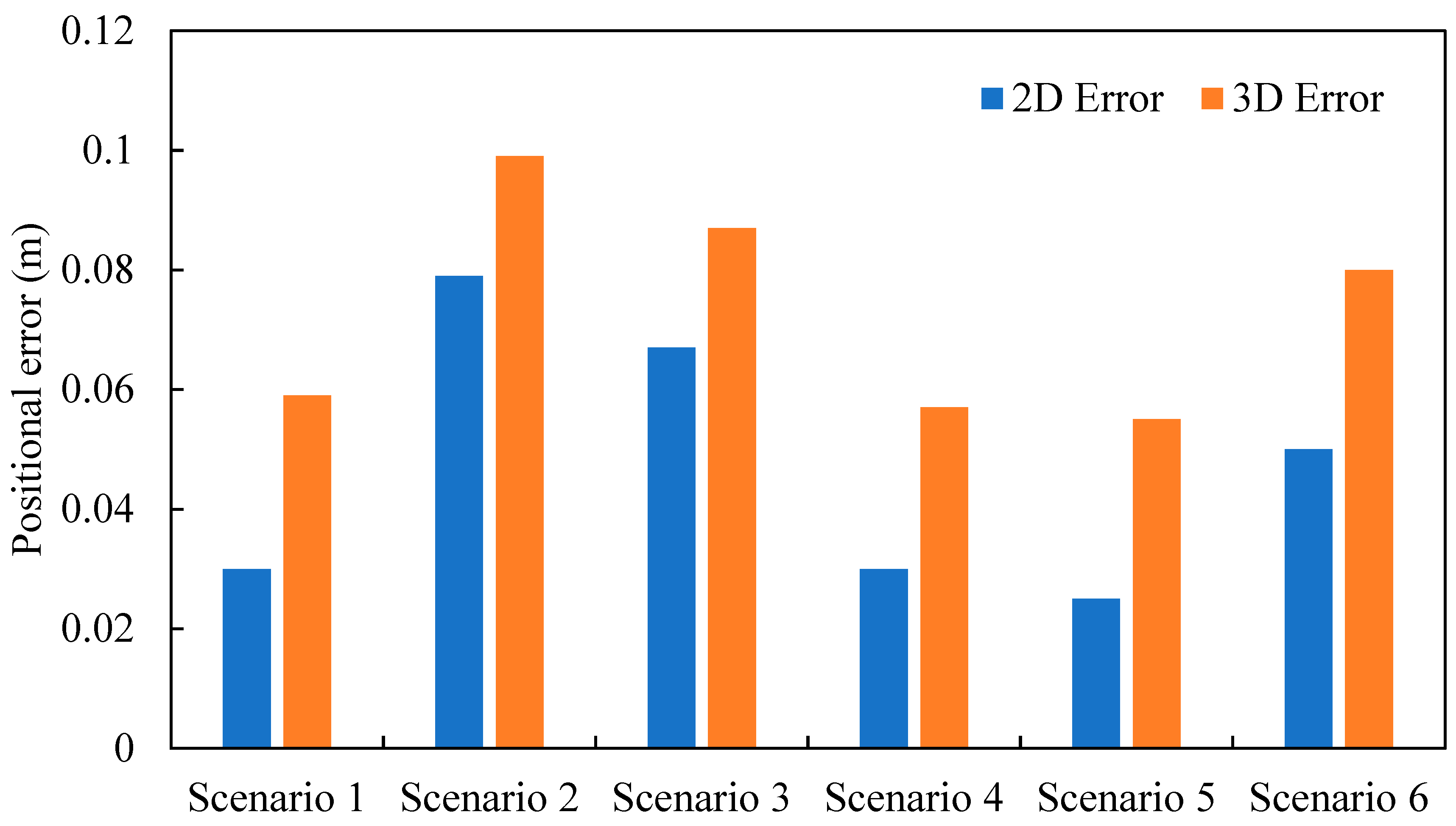
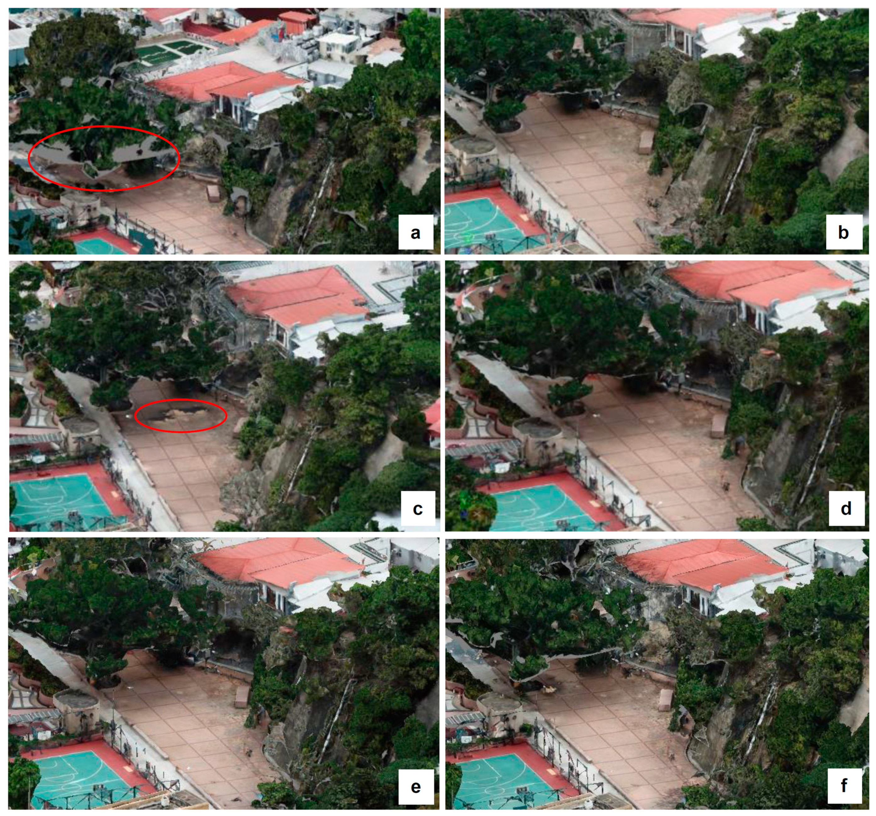
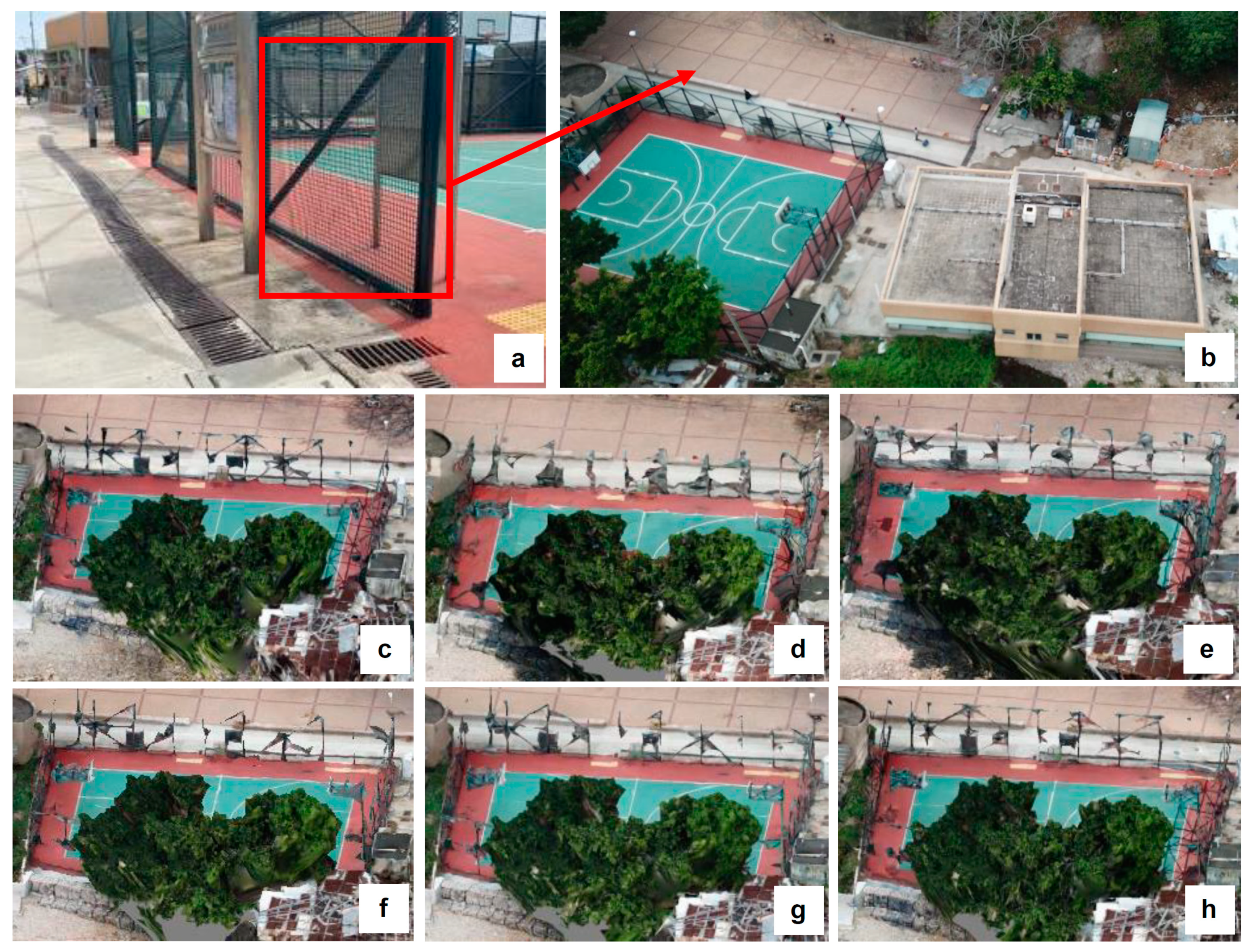
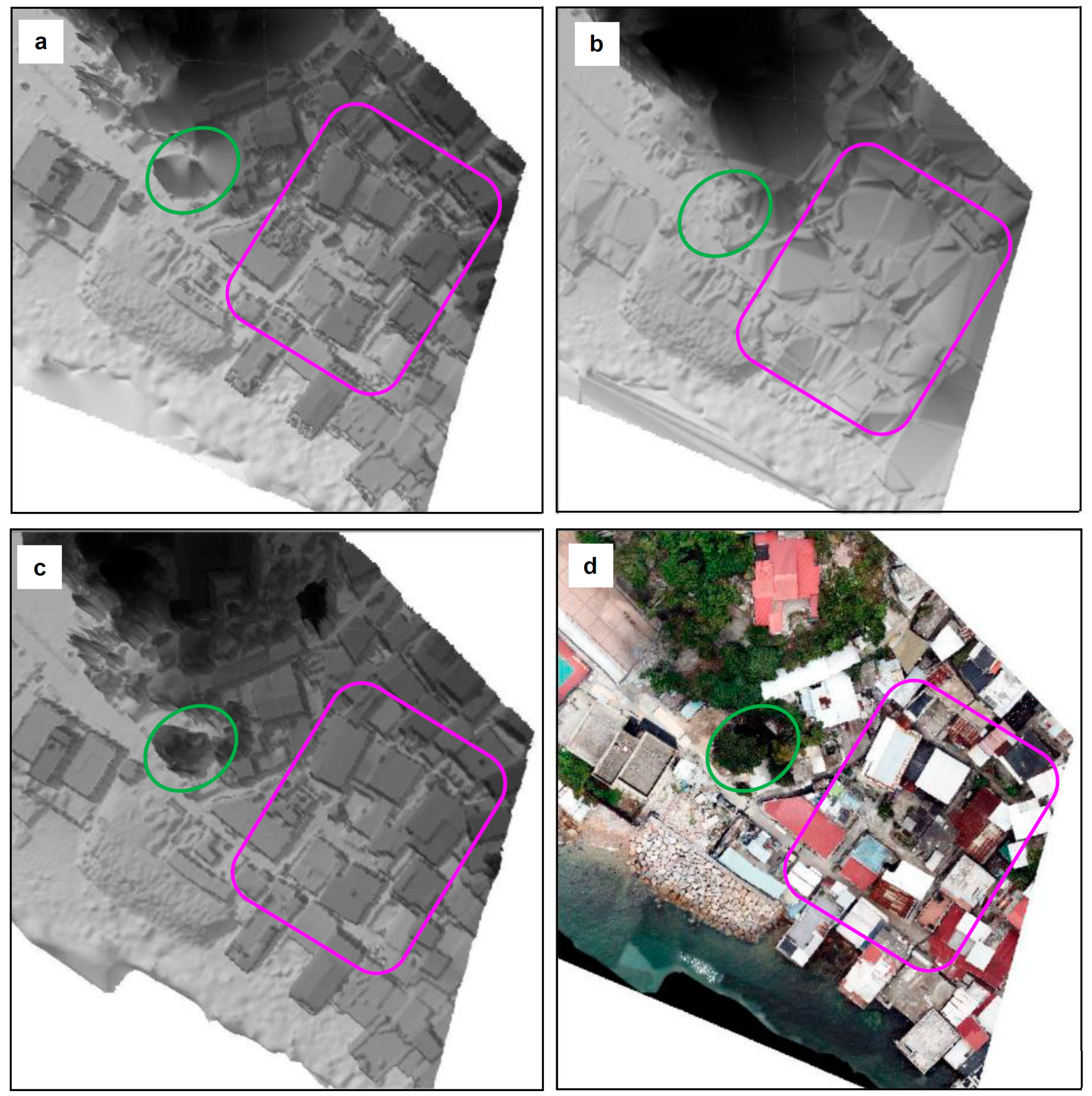
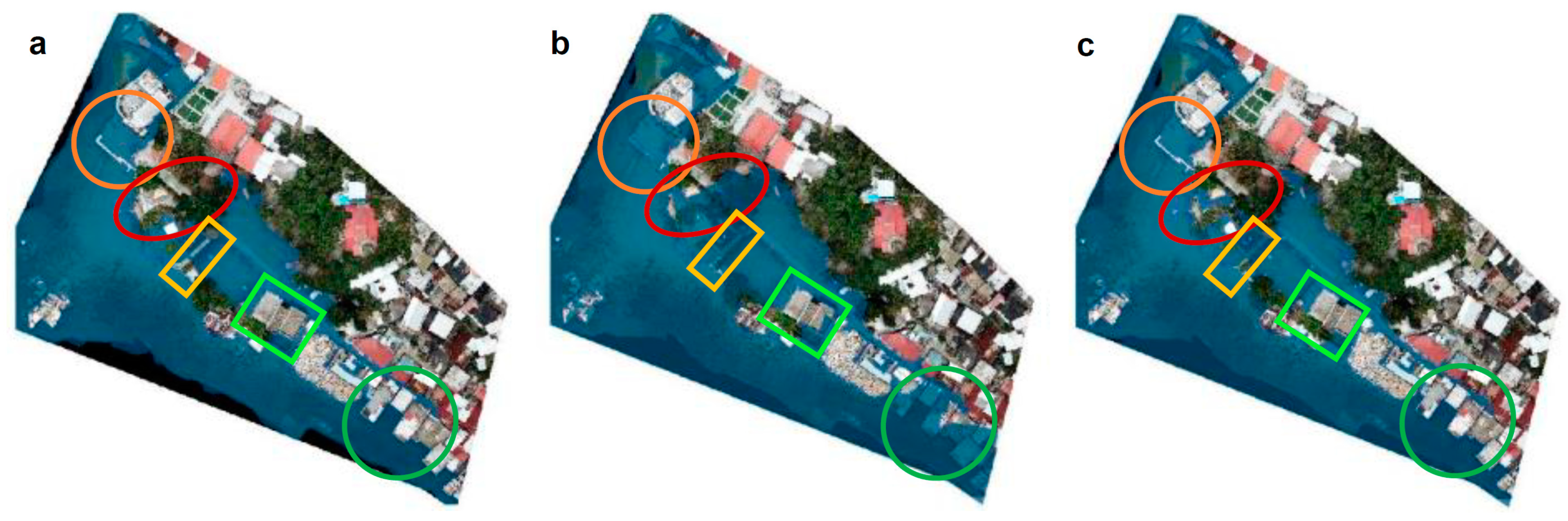
3.1. Accuracy Assessment and Texture Analysis of the 3D Mesh Model

Six 3D mesh models were generated following the designed scenarios setting shown in Table 1. Scenarios 1–3 were generated based on the single camera angle dataset while Scenarios 4–6 utilized the combined camera angle dataset. Figure 4 presents the 2D positional and 3D positional errors in the 3D mesh model for each scenario, irrespective of the surface type. The best case, Scenario 5, obtained an accuracy of ±2.7 cm and ±5.5 cm, respectively, in the 2D and 3D positions; while the worst case, Scenario 2, obtained ±7.9 cm and ±9.9 cm, respectively. Particularly, the accuracy assessment of the six scenarios demonstrated a common error pattern, in which the UAV-derived mesh model tended to overestimate the northing and elevation of points after comparing their mean residuals in northing, easting and height.
The resulting 3D model not only needed to be accurate in geometry but also needed to be a high level of detail in visual fidelity. Generally, it was not a big concern for commercial-grade UAVs to capture the details of flat areas or ground features and construct a model. However, it was more challenging to collect the building texture information such as roof and side walls and map the vegetated areas. Figure 5 presents a comparison of the vegetation visualization among different sets of photo combinations. Specifically, Scenario 1 (Figure 5a) led to various holes since the nadir images looked down to the terrain. The tree branches and tree trunks were the blind spots to the vertical camera view, which caused insufficient feature overlaps across the nadir images. Therefore, the tree features were not extracted and identified when the feature overlap was low, thereby leaving a data gap in the model. Scenarios 2 and 6 (Figure 5b,f) also had missing parts around the tree canopies, although they led to less information loss than Scenario 1. This may be attributed to an incomplete coverage of those areas, causing an inadequate number of matched key points between the images. Flaws were found in Scenario 3 (Figure 5c) as the wrong visualization of the ground texture was generated. It had some dark shadows appearing on the ground which meant the software had confusion in the texture information between the tree canopies and the ground and mismatched the tree texture with the tiles, therefore, failing to produce visually correct models. Scenarios 4 and 5 (Figure 5d,e) confirmed that the integration of the high and low oblique aerial images can provide a more complete image coverage and preserve the scene complexity.
To conclude, Scenario 5 (Figure 5e) was the optimal flight path to produce the photogrammetric model with relatively high accuracy and realistic digital documentation for this study area. It also required less battery to support the whole data capture in the study area compared to Scenario 6 (Figure 5f), which adopted a circular flying mode. It can be used for mapping textures on the 3D models of the study area without a great loss of visual quality. The above accuracy and texture assessment revealed that the production of a realistic 3D mesh model is dependent on the viewing angle of the camera. The integration of the images with different camera angles can supplement one another and provide more comprehensive and descriptive details of features on-site.
In addition, a common problem associated with these six scenarios was also identified. That is, all of the six scenarios are incapable of reconstructing the fence which appeared somewhat distorted (Figure 6). Figure 6a,b shows the appearance of the playground taken by cellphone. Figure 6c–h illustrates this common error arising in each scenario. This common mistake could be explained by the characteristic of the fences since they are not sharp features, which renders it challenging to recognize and detect from the images. Although the multiple camera angle image dataset had a desirable reconstruction in the buildings and the ground, which are the common feature types of the study area, it still had a minor problem That is, the aerial images acquired for this study led to an unsatisfactory performance in the reconstruction of the fine and indistinct features. Since the lowest flying height used in this study was 35 m, the fence details were still too small for the camera to capture. However, with the safety flying concern, the UAV was unable to fly lower than this minimum flying height to carry out a data capture mission without crashing into the trees.

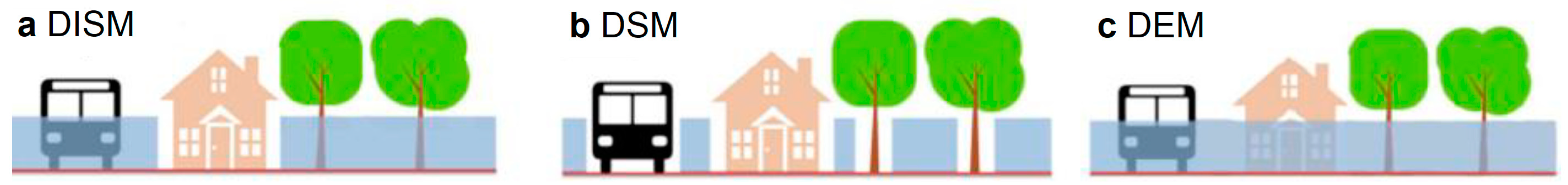
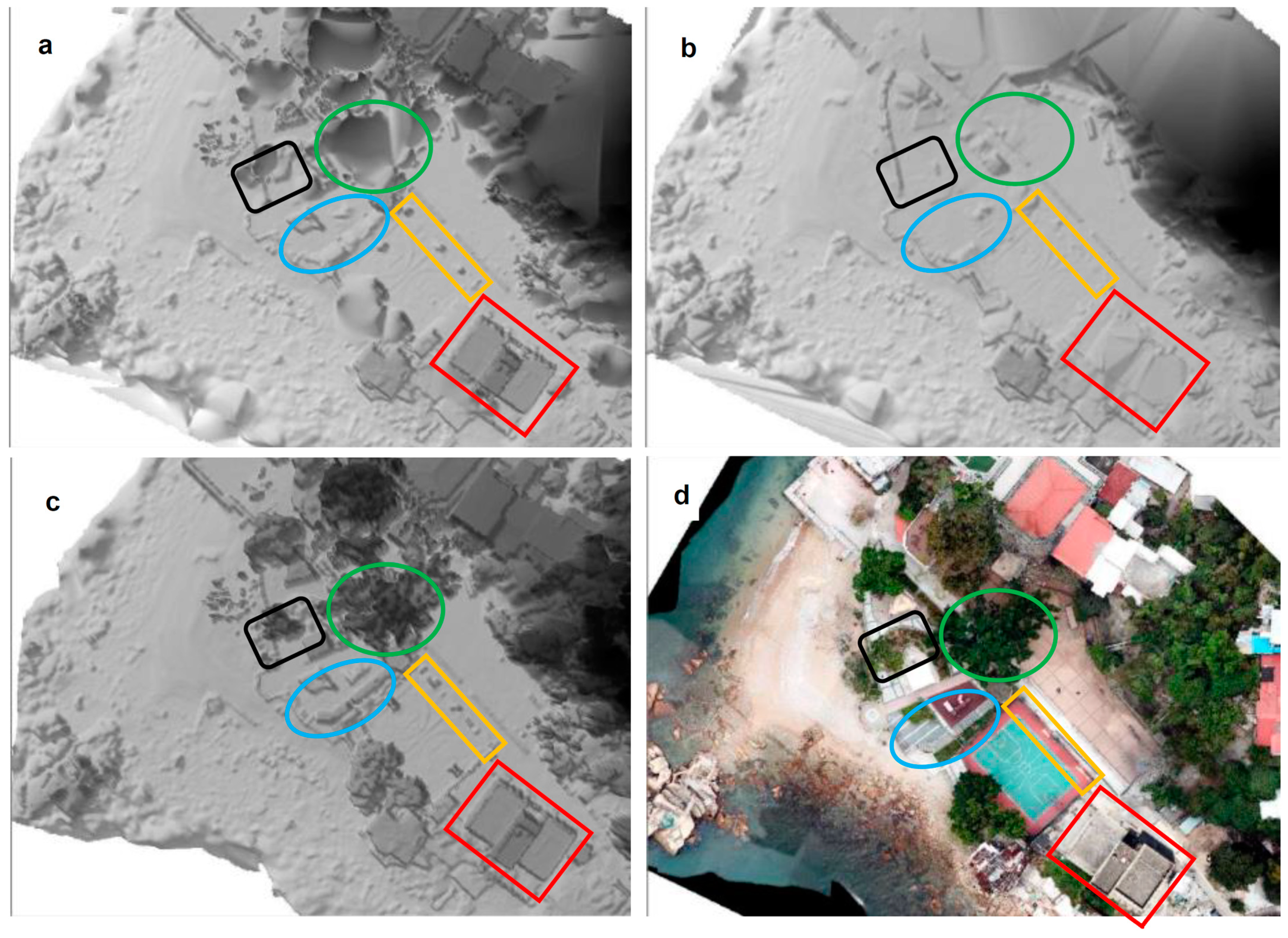
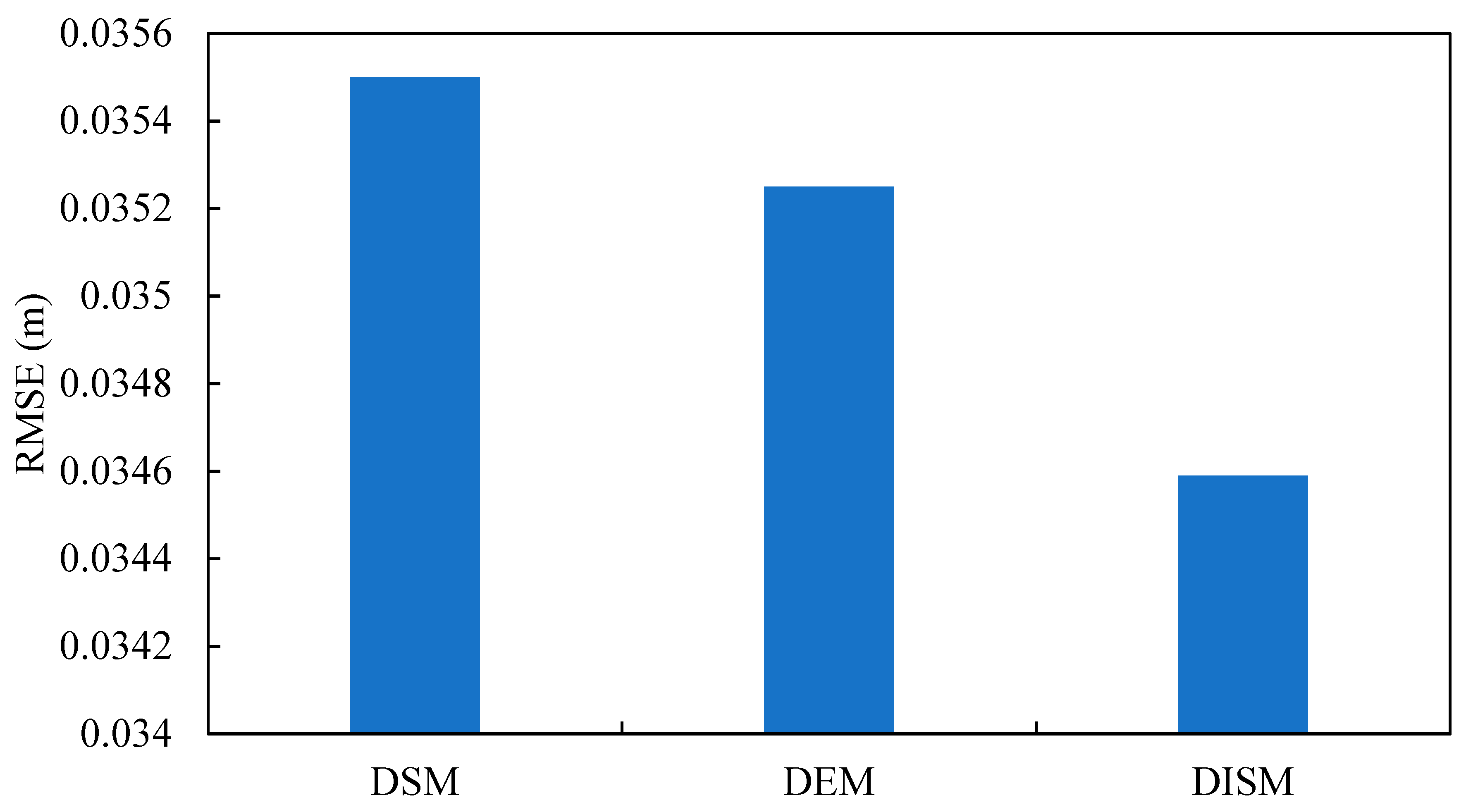
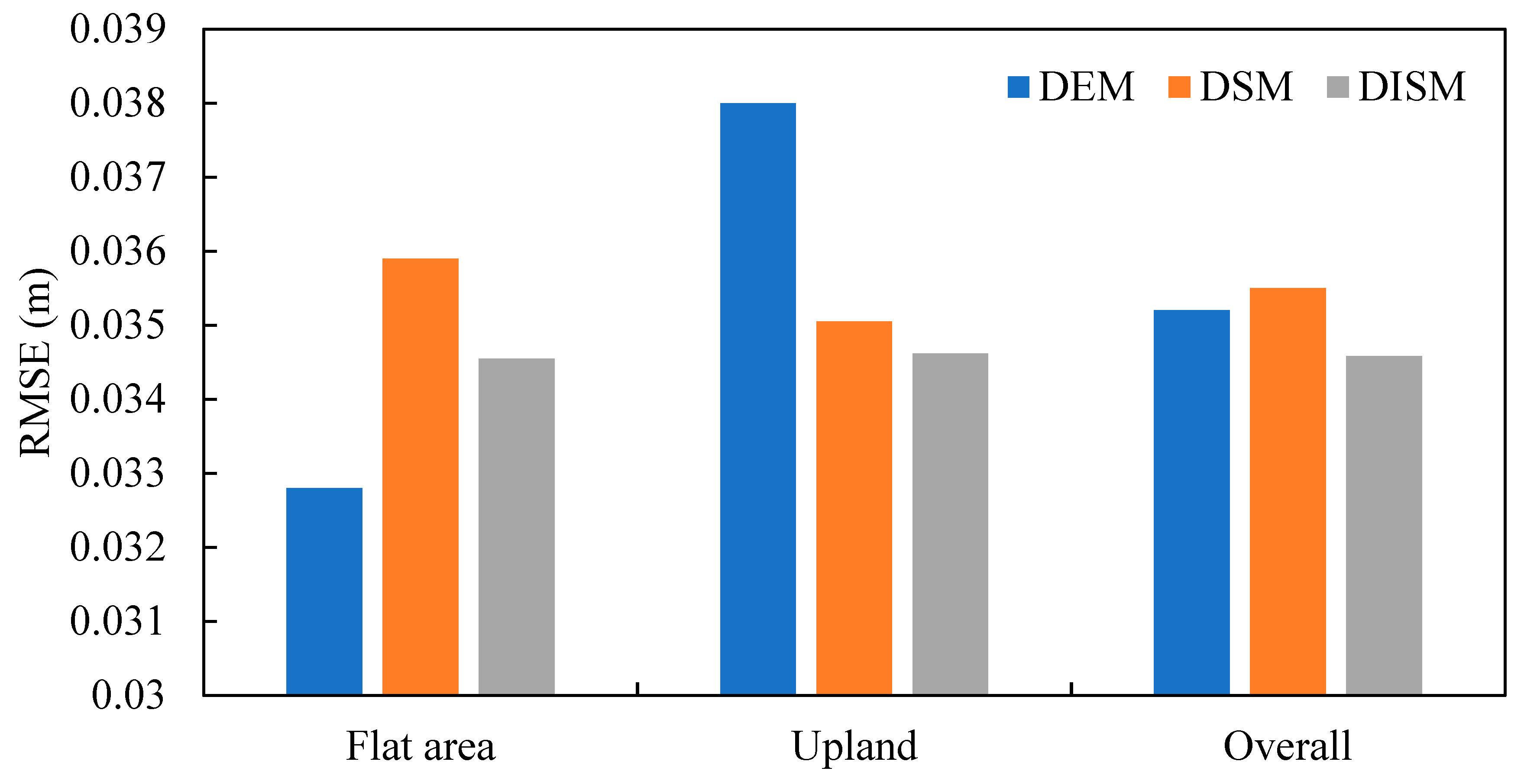
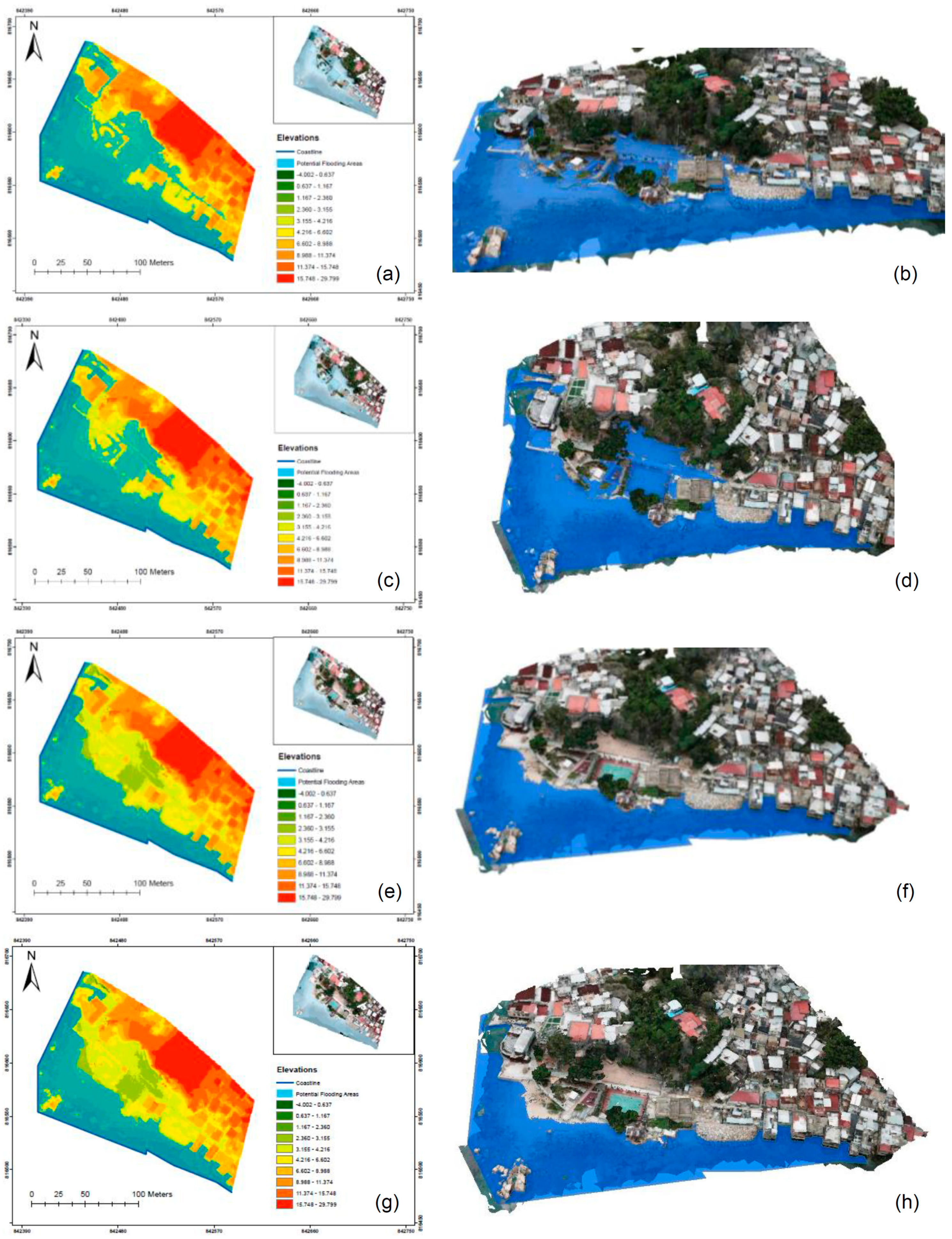
3.2. Comparison of the DISM, DSM and DEM

The study area was a topographically complex region, consisting of dense small houses, few recreational facilities and vegetation. Under this urban setting, both the DEM and the DSM had limitations in a hydrological application (see Figure 7). For example, the DSM retained the vegetated areas and was not able to account for the water inflow in areas which are under the cover of tree canopies (Figure 7b); whereas the DEM excluded all the artificial and impervious features (Figure 7c), which led to an inconsistency between the simulation result and the real-life condition as the buildings will not be covered or flooded with water unless the water level is higher than the height of the building roof. Moreover, some temporary features and fences in the study area should be removed since the fences allow water to pass through. The DISM was designed to represent the vulnerability of the existing structures to flood-related risks in a better extent since it struck a balance between the DSM and the DEM in terms of the nature of the terrain representation and kept additional data such as the features that may affect flood water flow (Figure 7a).
Figure 8 and Figure 9 present the visual differences between the DEM, DSM and DISM. The top views of the DSM, DEM, DISM and orthophoto were extracted in order to compare their visual differences in particular areas. The building outline can be seen clearly in both the DSM and the DISM, while the buildings have been removed and observed as a flat area in the DEM (see Figure 8). The planter was also kept in the DSM and the DISM as it has a similar function as the buildings. As they are slightly elevated above the surrounding terrain, they can block the stormwater and prevent it from running across the planter, affecting the direction of water flow. The vegetation was removed in the DEM and the DISM. In this vegetated area, multiple elevation values were presented at the same location such as tree canopy elevations and ground elevations. If the tree features are kept, this area will be depicted by the height of vegetation. Then, the software may falsely select the highest elevation in this area, the tree height, to compare with the projected sea level. It may overlook the elevation of the cells masked by the tree canopies as the water may flow underneath the tree canopies. Therefore, it cannot support the simulation of an accurate and realistic flooding scene. The fence and canopies in the park are classified as permeable features as the stormwater will be able to run through them and enter the inland areas. Therefore, they should be removed since the software cannot account for their permeability in the flooding analysis. The roads and buildings have a significant division as depicted in the DISM and the DSM; while the roads are a bit sketchy and less clear in the DEM (see Figure 9). Since the vegetation was removed in the DEM (depicted in yellow circle), the elevations of this area were computed by interpolation. This interpolated area was a bit fuzzy and low level in detail compared to the DSM, owing to the gradual inclination between the areas under the trees and retained building structures which might result in poor interpolation.
In addition to the visual inspection, a comparison of the statistical vertical errors for the DISM, DSM and DEM models is presented in Figure 10. The results show that the DSM, DEM and DISM obtained values of ±0.0355 m, ±0.0353 m and ±0.0346 m in the RMSE, regardless of the topographic characteristics. They tended to overestimate the height of the checkpoints. The largest difference between them was 0.9 mm which reflects that they attained similar quality. The standard deviation of the vertical discrepancies was also computed and compared. The DSM had the lowest standard deviation value which means the residuals measured from each checkpoint were less dispersed. Then, it can be assumed that the vertical errors associated with the rest of the cells over the entire DSM surface will have similar error magnitudes. Moreover, the standard deviation of the DEM and the DISM was more or less the same, only 3 mm away from the DSM standard deviation which implies that the performance was satisfactory. This suggests that the residuals with extreme values and variations, exceptionally large or small discrepancies in height, can barely be found within the same dataset, so the measurement precision in these products is relatively high. Therefore, it is reliable to adopt these three models in the coastal flooding analysis.
We also classified the checkpoints into two types and assessed the RMSE in the flat areas and the upland in order to better understand the influence of land surface cover on the accuracy of the DSM, DEM and DISM (see Figure 11). The largest RMSE difference between the flat areas and the upland was noted in the DEM, while the smallest RMSE difference was obtained in the DISM. The DSM RMSE values were ± 0.03589 m and ± 0.03503 m for the flat areas and upper areas, respectively. The difference between these two surface types was 1 mm at most and, therefore, was negligible. This small difference reflects that the elevated features show better accuracy than the flat ground. Generally, the accuracy of the DSM depends on the generated point cloud accuracy. Any obstruction of the tree canopies, insufficiency of overlapping images and mismatching of the building roof might lower the possibility of a trustable point cloud extraction from the images, accounting for the sources of vertical error. For the DEM, Figure 11 suggests that the checkpoints located on the upland have higher a RMSE than on flat areas and has a negative impact on the overall RMSE result. Fortunately, the RMSE of these two types was not significantly different. This difference can be explained by the interpolation error. Those checkpoints located on the upland were close to the built-up areas and all of the buildings and manmade features were removed from the point cloud dataset. When the software needs to construct a continuous raster surface from the discrete point clouds, it requires interpolation. With comparably fewer available point clouds, the interpolation of the DEM in this case tended to be less accurate, causing relatively larger vertical discrepancies in the upland checkpoints. For the DISM case, the RMSE errors in flat areas and upper areas were similar. It implies that the ranges of the DISM elevation discrepancies within each cell were quite stable over the area, with an average of about 3 cm. Most of the buildings and impermeable structures were retained in the DISM and these denser point clouds allowed for a finer representation of some spatial objects. The interpolation of the elevation in each cell was easier than the DEM as well since more feature point clouds were present for the software to interpolate the raster surface. This result shows that the DISM was almost independent of the surface characteristics.

3.3. Evaluation of the Seawater Inundation Simulations

It was important to examine the simulation performance in the DEM, DSM and DISM before deciding which elevation model would be adopted as the final data source in the storm surge analysis. Therefore, the three models were separately used to perform inundation simulations under the typhoon Mangkhut scenario and to examine whether the simulations were reasonable and realistic by the visual comparison. The orthophoto also assisted in the identification of the simulation defects. Figure 12 presents the flooding area calculated from the DSM, DEM, DISM and the simulation results are displayed on the orthophoto. The small houses pointed out in the green circle are flooded in the DEM while the DSM and the DISM are not inundated. The result in the DEM does not represent the real-life situation since the water will not run through the building unless the water level is higher than the building roofs, which are generally 7 m tall as measured in the 3D mesh model. Similar to the small house situation, the public toilet was partially inundated in the DEM only (see the green rectangle in Figure 12). It means that the DSM and the DISM can successfully take the building properties into account when performing the coastal flood analysis. The ground areas nearby the seaside (see the orange circle) were fully flooded in the DEM (Figure 12b) but were partially inundated in the DSM and the DISM. Such a partial inundation mapping generated from the DSM and the DISM resulted from the existence of the gabion walls in the inland areas (Figure 13a) and the walls replaced by the fence on the other side (Figure 13b). The fence causes the seawater to flow into the low-lying coastal areas and reduces the functionality of the gabion wall. The yellow rectangle highlights a false identification of the non-inundation zone for the permeable park canopy in the DSM only since this canopy fails to prevent from seawater running across at its bottom (see Figure 12a). Therefore, the DISM is the best terrain representation and model for the use of the storm surge analysis compared to the DEM and the DSM since it resolves the flooding vulnerability and resistance of each feature.
The 2018 flood event brought by Typhoon Mangkhut was used to explain the validation procedures adopted in this study. The DISM cells that were simulated to be submerged were rendered by deep blue colors based on the maximum inundation depths. Figure 14 shows that the flooded cells mainly propagate along streets and accumulate in the southern sides of the study area, which have low-lying topographies and are generally consistent with the infusion zone observed from the aforementioned documentation within regions A–D in this flood event. The remarkable differences between the simulated inundation area and the actual circumstance occurred at locations near the recreational facilities in flooding Zone B. The discrepancies in the simulations of the localized inundation areas were attributed to the discontinuity of the flooded grid cells. Since some of the grid cells in Region B were adjacent to the flower bed and some solid obstructions that have higher elevations than the nearby ground elevations, the interpolated result was greatly influenced by these extreme values. Sometimes the small mistakes in interpolation might cause a large error in the height value of each grid cell. If the elevation of the grid cells varies from the neighboring cells and exceeds the range of the particular water level, it may break the connectivity and it will not be treated as flooding. Additionally, it does not take the water accumulation and flow along the streets and other lowlands into consideration, which in turn leads to a less realistic flood modeling result and underestimation of the flood extent.
Figure 15 presents the inundation simulations under the four major typhoon events, including Typhoon Mangkhut in 2018, Typhoon Hato in 2017, Typhoon Wipha in 2013 and Typhoon Higos in 2020. Table 2 summarizes the simulation performance of the DISM in the different scenarios of the typhoon-induced storm surges. It appeared that the simulated flooding zones were characterized by an acceptable degree of consistency among all the testing scenarios. The proposed DISM can attain a successful simulation rate of 90% in most of the modeling scenarios which appropriately satisfies its design function, depicting the areas prone to seawater infusion under different sea level scenarios. This validation test assures the reliability of the simulation result produced from the proposed DISM.

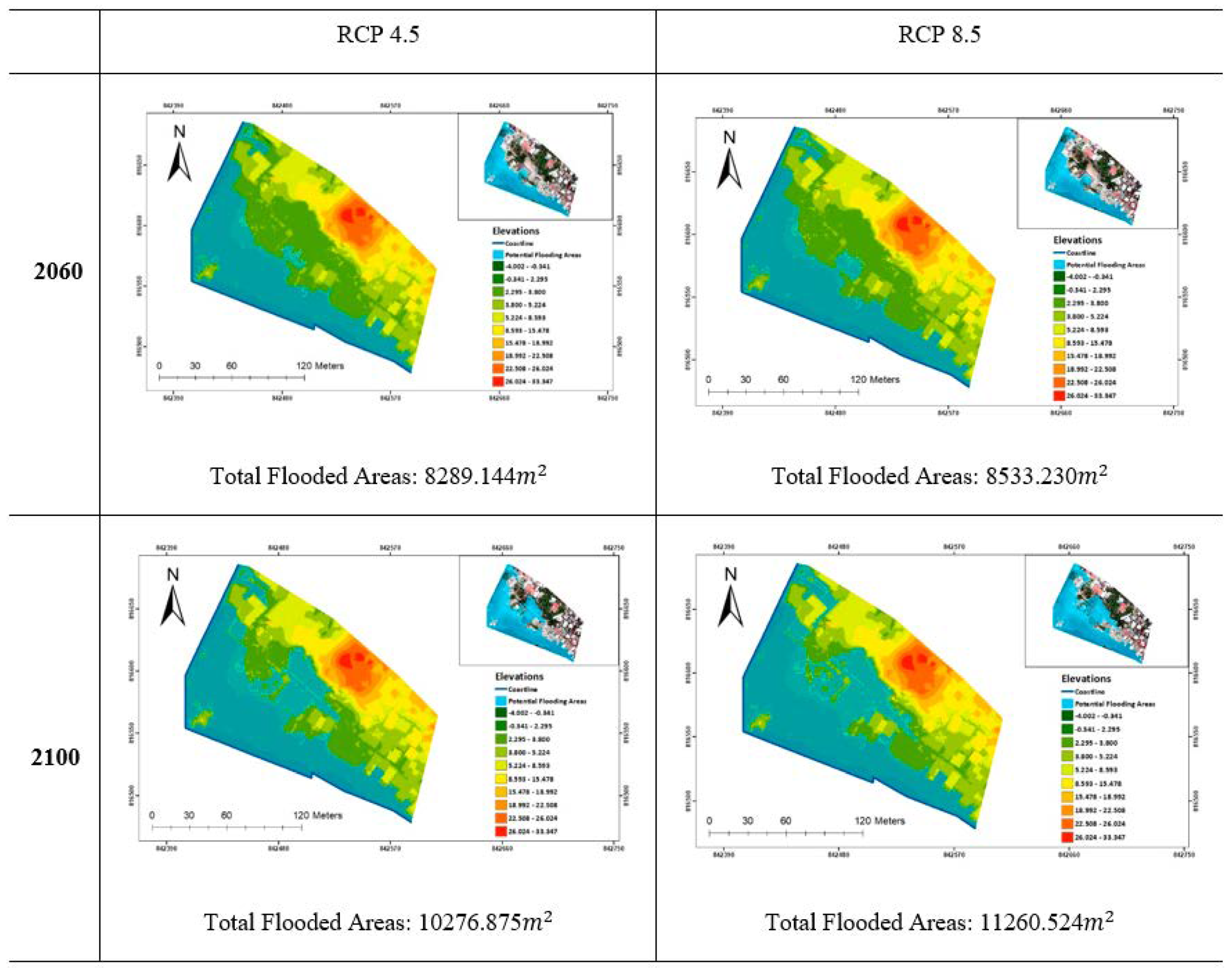
3.4. Projection of Coastal Flooding

With the anticipated further increase in atmospheric greenhouse gases in the next few decades, the rate of sea-level rise will drastically accelerate, leaving coastal communities exposed to devastating circumstances. This study took the worst-case local scenarios provided by the Hong Kong Observatory (HKO), which predicts the mean sea level changes under the representative concentration pathway (RCP) 4.5 and the RCP8.5 scenarios by 2050 and 2100, respectively (see Figure 16 and Table 3). The results show that the water level of Victoria’s Harbor will rise to 2.995 m above the Hong Kong Principal Datum (mPD) and 3.335 mPD in the future periods of 2051–2060 and 2091–2100, respectively, under the RCP4.5. Nevertheless, the water level would rise to 3.055 mPD and 3.605 mPD by 2060 and 2100 if greenhouse gas emissions escalated to the RCP8.5. It is noticeable to observe the effect of sea level rise, specifically on land subsistence [40]. The sea level near Victoria Harbor will rise by as much as 40 and 100 cm, respectively, relative to its present value under the RCP4.5 and the RCP8.5. This represents a large increase in the baseline sea level and most of the inland areas of the Man Wan village will be submerged in this century. When an abnormal rising sea level event happens, such as a storm surge, the flood vulnerability will be magnified, causing huge human and economic losses. In addition, we also observe that the projected mean sea level will lead to a substantial inundation in the study area under the RCP4.5 and the RCP8.5. Specifically, the bathtub-based simulations show that the total inundation areas are projected to be up to 8,200 square meters, which is comparable with those induced by Typhoon Wipha and Typhoon Higos by 2060 under both emission scenarios. The total inundation areas would increase to up to 10,200 square meters by 2100, which is comparable with those induced by Typhoon Mangkhut and Hato. It should be noted that such an inundation projection is solely based on the mean sea level and the risks would further increase if the projected extreme sea level was taken into account [41,42,43,44,45,46,47,48,49,50,51].

4. Conclusions

This study connects fieldwork to numerical modeling, which offers both practical and theoretical contributions to coastal flood exposure, vulnerability and risk assessment at community levels. We propose a new elevation model named the DISM to improve the characterization of seawater inundation induced by typhoon-induced storm surges and extreme sea levels. This model was constructed based on the topographical data acquired by a UAV and was compared with the existing well-known DEM and DSM in terms of elevation accuracy and inundation mapping based on visual inspection and accuracy assessment. A bathtub method that considers the surface connectivity and employs the DISM as an input was used to characterize the seawater inundation induced by four significant typhoons and was evaluated by comparing the simulated and observed inundation area. In addition, the DISM-based bathtub method was used to project coastal flood risks under the RCP4.5 and the RCP8.5.
The proposed DISM improves upon the existing DEM and DSM with a relatively low RMSE of ±0.035 m. Such a model also improves upon the DEM and the DSM in terms of seawater inundation mapping by filtering the temporary and permeable features and retaining the impermeable features. Our findings show that the DSM and the DISM can successfully take the building properties into account when performing the coastal flood analysis, but the DSM may not characterize the temporary and porous structures. The proposed DISM can reach a high reliability of almost 90% in mapping the areas prone to seawater infusion under different sea level scenarios. Sea level rise is projected to cause inundation for areas as many as those induced by severe typhoons (e.g., wind speeds reach 150 km/h) by 2060 under the RCP4.5 and the RCP8.5. Such an intensification of coastal inundation risk would be further magnified and compared to those induced by super typhoons (e.g., wind speeds reach 185 km/h) by 2100. Climate change impact is prevalent nowadays. If the situation continuously deteriorates, the waterfront areas of the study area will suffer from seawater inundation more frequently. These findings not only can help policymakers identify the low-lying locations that are vulnerable to seawater inundation and formulate improvement works, but also raise awareness of the flooding risks and prevention among the residents. Since the existing seawall and gabion walls can be overtopped by seawater caused by extreme storm surges with longer return periods, authorities should re-examine the flood protection measures to strengthen the flood resilience in the study area. The outcomes of this study provide meaningful insights for relevant flood prevention service providers to carry out inspections of flooding blackspots with the use of this less manpower-intensive and time-consuming surveying technology. The elevation model used in this study can also be directly applicable to various hydrologic studies and engineering projects in coastal cities around the world. Since extreme sea level events commonly lead to substantial economic damages, it is also desired to use the proposed elevation model for improving the estimation of the economic damages associated with coastal inundation in future studies.
It should be noted that the proposed DISM was generated by extracting the water-permeable features manually, which provided a highly reliable feature extraction. However, it was time-consuming and labor-intensive. Although the UAV-based DISM led to a higher performance than the existing DEM and DSM, the UAV was incapable of penetrating the ground surface surrounded by dense vegetation. With computer technology advancement, integrating AI techniques in the development of the DISM would become a key research focus in the future. AI technologies can automatically detect and segment those impervious features from the original DSM.

Author Contributions

Conceptualization, S.W.; Methodology, Y.S., B.Z. and C.Y.C.; Software, B.Z. and C.Y.C.; Validation, Y.S., B.Z. and C.Y.C.; Formal analysis, Y.S., B.Z. and C.Y.C.; Investigation, C.Y.C. and S.W.; Resources, S.W.; Data curation, C.Y.C.; Writing—original draft, Y.S., B.Z. and C.Y.C.; Writing—review & editing, S.W.; Visualization, B.Z. and C.Y.C.; Supervision, S.W.; Project administration, S.W.; Funding acquisition, S.W. All authors have read and agreed to the published version of the manuscript.

Funding

This research was supported by the Environment and Conservation Fund (P0038498), the LSGI Collaborative Research Grant (P0036639) and the Smart Cities Research Institute Fund (P0043554).

Institutional Review Board Statement

Not applicable.

Informed Consent Statement

Not applicable.

Data Availability Statement

Projected mean sea level changes were collected from the Hong Kong Observatory, which can be found here: https://www.hko.gov.hk/en/climate_change/proj_hk_msl_med_conf_info.htm (accessed on 9 April 2022).

Acknowledgments

The authors are pleased to express their gratitude to the two anonymous reviewers of the manuscript for valuable and helpful comments.

Conflicts of Interest

The authors declare no conflict of interest.

References

  1. Zhang, B.; Wang, S. Probabilistic characterization of extreme storm surges induced by tropical cyclones. J. Geophys. Res. Atmos. 2021, 126, e2020JD033557. [Google Scholar] [CrossRef]
  2. Nicholls, R.J.; Lincke, D.; Hinkel, J.; Brown, S.; Vafeidis, A.T.; Meyssignac, B.; Hanson, S.E.; Merkens, J.-L.; Fang, J. A global analysis of subsidence, relative sea-level change and coastal flood exposure. Nat. Clim. Chang. 2021, 11, 338–342. [Google Scholar] [CrossRef]
  3. Gutmann, E.D.; Rasmussen, R.M.; Liu, C.; Ikeda, K.; Bruyere, C.L.; Done, J.M.; Garrè, L.; Friis-Hansen, P.; Veldore, V. Changes in hurricanes from a 13-yr convection-permitting pseudo- global warming simulation. J. Clim. 2018, 31, 3643–3657. [Google Scholar] [CrossRef]
  4. Yang, J.; Li, L.; Zhao, K.; Wang, P.; Wang, D.; Sou, I.M.; Yang, Z.; Hu, J.; Tang, X.; Mok, K.M.; et al. A comparative study of Typhoon Hato (2017) and Typhoon Mangkhut (2018)—Their impacts on coastal inundation in Macau. J. Geophys. Res. Ocean. 2019, 124, 9590–9619. [Google Scholar] [CrossRef]
  5. Gebrehiwot, A.A.; Hashemi-Beni, L. Three-dimensional inundation mapping using UAV image segmentation and digital surface model. ISPRS Int. J. Geo Inf. 2021, 10, 144. [Google Scholar] [CrossRef]
  6. Williams, L.L.; Lück-Vogel, M. Comparative assessment of the GIS based bathtub model and an enhanced bathtub model for coastal inundation. J. Coast. Conserv. 2020, 24, 23. [Google Scholar] [CrossRef]
  7. Kulp, S.A.; Strauss, B.H. New elevation data triple estimates of global vulnerability to sea-level rise and coastal flooding. Nat. Commun. 2019, 10, 4844. [Google Scholar] [CrossRef] [Green Version]
  8. Xu, K.; Fang, J.; Fang, Y.; Sun, Q.; Wu, C.; Liu, M. The Importance of digital elevation model selection in flood simulation and a proposed method to reduce DEM errors: A case study in Shanghai. Int. J. Disaster Risk Sci. 2021, 12, 890–902. [Google Scholar] [CrossRef]
  9. Karamuz, E.; Romanowicz, R.J.; Doroszkiewicz, J. The use of unmanned aerial vehicles in flood hazard assessment. J. Flood Risk Manag. 2020, 13, e12622. [Google Scholar] [CrossRef]
  10. Shen, J.; Tan, F.; Zhang, Y. Improved building treatment approach for urban inundation modeling: A case study in Wuhan, China. Water 2018, 10, 1760. [Google Scholar] [CrossRef]
  11. Parizi, E.; Khojeh, S.; Hosseini, S.M.; Moghadam, Y.J. Application of unmanned aerial vehicle DEM in flood modeling and comparison with global DEMs: Case study of Atrak river basin, Iran. J. Environ. Manage 2022, 317, 115492. [Google Scholar] [CrossRef] [PubMed]
  12. Annis, A.; Nardi, F.; Petroselli, A.; Apollonio, C.; Arcangeletti, E.; Tauro, F.; Belli, C.; Bianconi, R.; Grimaldi, S. UAV-DEMs for small-scale flood hazard mapping. Water 2020, 12, 1717. [Google Scholar] [CrossRef]
  13. Aral, M.M.; Chang, B. Spatial variation of sea level rise at Atlantic and Mediterranean coastline of Europe. Water 2017, 9, 522. [Google Scholar] [CrossRef] [Green Version]
  14. Griffin, J.; Latief, H.; Kongko, W.; Harig, S.; Horspool, N.; Hanung, R.; Rojali, A.; Maher, N.; Fuchs, A.; Hossen, J.; et al. An evaluation of onshore digital elevation models for modeling tsunami inundation zones. Front. Earth Sci. 2015, 3, 32. [Google Scholar] [CrossRef] [Green Version]
  15. Li, B.; Hou, J.; Li, D.; Yang, D.; Han, H.; Bi, X.; Wang, X.; Hinkelmann, R.; Xia, J. Application of LiDAR UAV for high-resolution flood modelling. Water Resour. Manag. 2021, 35, 1433–1447. [Google Scholar] [CrossRef]
  16. Kastridis, A.; Kirkenidis, C.; Sapountzis, M. An integrated approach of flash flood analysis in ungauged mediterranean watersheds using post-flood surveys and unmanned aerial vehicles. Hydrol. Process. 2020, 34, 4920–4939. [Google Scholar] [CrossRef]
  17. Yan, D.; Li, J.; Yao, X.; Luan, Z. Integrating UAV data for assessing the ecological response of spartina alterniflora towards inundation and salinity gradients in coastal wetland. Sci. Total Environ. 2022, 814, 152631. [Google Scholar] [CrossRef]
  18. Marks, K.; Bates, P. Integration of high-resolution topographic data with floodplain flow models. Hydrol. Process. 2000, 14, 2109–2122. [Google Scholar] [CrossRef]
  19. Castellarin, A.; Di Baldassarre, G.; Bates, P.D.; Brath, A. Optimal cross-sectional spacing in preissmann scheme 1D hydrodynamic models. J. Hydraul. Eng. 2009, 135, 96–105. [Google Scholar] [CrossRef]
  20. Muhadi, N.A.; Abdullah, A.F.; Bejo, S.K.; Mahadi, M.R.; Mijic, A. The use of LiDAR-derived DEM in flood applications: A review. Remote Sens. 2020, 12, 2308. [Google Scholar] [CrossRef]
  21. Pichon, L.; Ducanchez, A.; Fonta, H.; Tisseyre, B. Quality of digital elevation models obtained from unmanned aerial vehicles for precision viticulture. Oeno One 2016, 50, 101–111. [Google Scholar] [CrossRef] [Green Version]
  22. Dyer, J.L.; Moorhead, R.J.; Hathcock, L. Identification and analysis of microscale hydrologic flood impacts using unmanned aerial systems. Remote Sens. 2020, 12, 1549. [Google Scholar] [CrossRef]
  23. Munawar, H.S.; Ullah, F.; Qayyum, S.; Heravi, A. Application of deep learning on UAV-based aerial images for flood detection. Smart Cities 2021, 4, 1220–1243. [Google Scholar] [CrossRef]
  24. Wang, G.; Li, P.; Li, Z.; Ding, D.; Qiao, L.; Xu, J.; Li, G.; Wang, H. Coastal dam inundation assessment for the Yellow River Delta: Measurements, analysis and scenario. Remote Sens. 2020, 12, 3658. [Google Scholar] [CrossRef]
  25. Wang, X.; Xie, H. A review on applications of remote sensing and geographic information systems (GIS) in water resources and flood risk management. Water 2018, 10, 608. [Google Scholar] [CrossRef] [Green Version]
  26. Park, K.; Shibuo, Y.; Katayama, J.; Baba, S.; Furumai, H. Applicability of high-resolution geospatial data obtained by UAV photogrammetry to develop drainage system models for pluvial flood analysis. J. Disaster Res. 2021, 16, 371–380. [Google Scholar] [CrossRef]
  27. Trepekli, K.; Balstrøm, T.; Friborg, T.; Fog, B.; Allotey, A.N.; Kofie, R.Y.; Møller-Jensen, L. UAV-borne, LiDAR-based elevation modelling: A method for improving local-scale urban flood risk assessment. Nat. Hazards 2022, 113, 423–451. [Google Scholar] [CrossRef]
  28. Jakovljevic, G.; Govedarica, M.; Alvarez-Taboada, F.; Pajic, V. Accuracy assessment of deep learning based classification of LiDAR and UAV points clouds for DTM creation and flood risk mapping. Geosciences 2019, 9, 323. [Google Scholar] [CrossRef] [Green Version]
  29. Schumann, G.J.-P.; Muhlhausen, J.; Andreadis, K.M. Rapid mapping of small-scale river-floodplain environments using UAV SfM supports classical theory. Remote Sens. 2019, 11, 982. [Google Scholar] [CrossRef] [Green Version]
  30. Strauss, B.H.; Orton, P.M.; Bittermann, K.; Buchanan, M.K.; Gilford, D.M.; Kopp, R.E.; Kulp, S.; Massey, C.; de Moel, H.; Vinogradov, S. Economic damages from Hurricane Sandy attributable to sea level rise caused by anthropogenic climate change. Nat. Commun. 2021, 12, 2720. [Google Scholar] [CrossRef]
  31. Mazzoleni, M.; Paron, P.; Reali, A.; Juizo, D.; Manane, J.; Brandimarte, L. Testing UAV-derived topography for hydraulic modelling in a tropical environment. Nat. Hazards 2020, 103, 139–163. [Google Scholar] [CrossRef]
  32. He, Y.H.; Mok, H.Y.; Lai, E.S.T. Projection of sea-level change in the vicinity of Hong Kong in the 21st century. Int. J. Climatol. 2016, 36, 3237–3244. [Google Scholar] [CrossRef]
  33. Barba, S.; Barbarella, M.; Di Benedetto, A.; Fiani, M.; Gujski, L.; Limongiello, M. Accuracy assessment of 3D photogrammetric models from an unmanned aerial vehicle. Drones 2019, 3, 79. [Google Scholar] [CrossRef] [Green Version]
  34. Lingua, A.; Noardo, F.; Spanò, A.; Sanna, S.; Matrone, F. 3D model generation using oblique images acquired by UAV. Int. Arch. Photogramm. Remote Sens. Spat. Inf. Sci. 2017, XLII-4/W2, 107–115. [Google Scholar] [CrossRef] [Green Version]
  35. Nesbit, P.; Hugenholtz, C. Enhancing UAV–SfM 3D model accuracy in high-relief landscapes by incorporating oblique images. Remote Sens. 2019, 11, 239. [Google Scholar] [CrossRef] [Green Version]
  36. Seifert, E.; Seifert, S.; Vogt, H.; Drew, D.; van Aardt, J.; Kunneke, A.; Seifert, T. Influence of drone altitude, image overlap, and optical sensor resolution on multi-view reconstruction of forest images. Remote Sens. 2019, 11, 1252. [Google Scholar] [CrossRef] [Green Version]
  37. Nagendran, S.K.; Tung, W.Y.; Mohamad Ismail, M.A. Accuracy assessment on low altitude UAV-borne photogrammetry outputs influenced by ground control point at different altitude. In IOP Conference Series: Earth and Environmental Science, Proceedings of the 9th IGRSM International Conference and Exhibition on Geospatial & Remote Sensing (IGRSM 2018), Kuala Lumpur, Malaysia, 24–25 April 2018; IOP Publishing: Bristol, UK, 2018; Volume 169, p. 012031. [Google Scholar]
  38. Mesas-Carrascosa, F.J.; García, M.D.N.; De Larriva, J.E.M.; García-Ferrer, A. An Analysis of the influence of flight parameters in the generation of unmanned aerial vehicle (UAV) orthomosaicks to survey archaeological areas. Sensors 2016, 16, 1838. [Google Scholar] [CrossRef] [Green Version]
  39. Gallagher, J. Learning about an infrequent event: Evidence from flood insurance take-up in the United States. Am. Econ. J. Appl. Econ. 2014, 6, 206–233. [Google Scholar] [CrossRef] [Green Version]
  40. Hu, B.; Chen, J.; Zhang, X. Monitoring the land subsidence area in a coastal urban area with InSAR and GNSS. Sensors 2019, 19, 3181. [Google Scholar] [CrossRef] [Green Version]
  41. Calafat, F.M.; Marcos, M. Probabilistic reanalysis of storm surge extremes in Europe. Proc. Natl. Acad. Sci. USA 2020, 117, 1877–1883. [Google Scholar] [CrossRef]
  42. Zhu, J.; Wang, S.; Huang, G. Assessing climate change impacts on human-perceived temperature extremes and underlying uncertainties. J. Geophys. Res. Atmos. 2019, 124, 3800–3821. [Google Scholar] [CrossRef]
  43. Zhang, B.; Wang, S.; Wang, Y. Copula-based convection-permitting projections of future changes in multivariate drought characteristics. J. Geophys. Res. Atmos. 2019, 124, 7460–7483. [Google Scholar] [CrossRef]
  44. Wang, S.; Wang, Y. Improving probabilistic hydroclimatic projections through high-resolution convection-permitting climate modeling and Markov chain Monte Carlo simulations. Clim. Dyn. 2019, 53, 1613–1636. [Google Scholar] [CrossRef]
  45. You, J.; Wang, S. Higher probability of occurrence of hotter and shorter heat waves followed by heavy rainfall. Geophys. Res. Lett. 2021, 48, e2021GL094831. [Google Scholar] [CrossRef]
  46. Qing, Y.; Wang, S.; Ancell, B.C.; Yang, Z.-L. Accelerating flash droughts induced by the joint influence of soil moisture depletion and atmospheric aridity. Nat. Commun. 2022, 13, 1139. [Google Scholar] [CrossRef]
  47. Qing, Y.; Wang, S. Multi-decadal convection-permitting climate projections for China’s Greater Bay Area and surroundings. Clim. Dyn. 2021, 57, 415–434. [Google Scholar] [CrossRef]
  48. Li, X.; Wang, S. Recent increase in the occurrence of snow droughts followed by extreme heatwaves in a warmer world. Geophys. Res. Lett. 2022, 49, e2022GL099925. [Google Scholar] [CrossRef]
  49. Chen, H.; Wang, S.; Wang, Y.; Zhu, J. Probabilistic projections of hydrological droughts through convection-permitting climate simulations and multimodel hydrological predictions. J. Geophys. Res. Atmos. 2020, 125, e2020JD032914. [Google Scholar] [CrossRef]
  50. Chen, H.; Wang, S. Accelerated transition between dry and wet periods in a warming climate. Geophys. Res. Lett. 2022, 49, e2022GL099766. [Google Scholar] [CrossRef]
  51. Zhang, B.; Wang, S.; Qing, Y.; Zhu, J.; Wang, D.; Liu, J. A vine copula-based polynomial chaos framework for improving multi-model hydroclimatic projections at a multi-decadal convection-permitting scale. Water Resour. Res. 2022, 58, e2022WR031954. [Google Scholar] [CrossRef]
Figure 1. (a) The study area and distribution of the ground control points and checkpoints. The inset map in (a) shows the location of the study area in Hong Kong. (b) The outline map of buildings and constructions in the study area.
Atmosphere 14 00052 g001
Figure 2. Site inspection for flight planning. (A) Heavily vegetated area and (B) confined area in the study area.
Atmosphere 14 00052 g002
Figure 3. Reconstruction result of using (a) vertical photos, (b) oblique photos and (c) integrated vertical and oblique photos.
Atmosphere 14 00052 g003
Figure 4. Comparison of the 2D errors and 3D errors in the 3D mesh model for each scenario.
Atmosphere 14 00052 g004
Figure 5. Visualization of vegetation in (af) Scenarios 1–6. The red circles in (a,c) represent the missing parts.
Atmosphere 14 00052 g005
Figure 6. Texture analysis of a playground. (a,b) The ground-based view and the UAV aerial photo of the playground. (ch) The fences of the playground generated under six scenarios.
Atmosphere 14 00052 g006
Figure 7. Graphical illustration of the differences between (a) DISM, (b) DSM and (c) DEM.
Atmosphere 14 00052 g007
Figure 8. Comparison of (a) the DISM, (b) DEM, (c) DSM and (d) the orthophoto in terms of the different features. The red and black rectangles represent buildings and planters, respectively, that are filtered in (b) the DEM. The blue, green and orange circles represent permeable structures, vegetation and the fence, respectively, that are filtered in (a) the DISM and (b) the DEM.
Atmosphere 14 00052 g008
Figure 9. Comparison of (a) the DISM, (b) the DEM, (c) the DSM and (d) the orthophoto in terms of vegetation (green circle) and roads between small houses (purple rectangle).
Atmosphere 14 00052 g009
Figure 10. Comparison of the root mean square error (RMSE) in the DSM, DEM, and DISM at all the checkpoints.
Atmosphere 14 00052 g010
Figure 11. Comparison of the root mean square error (RMSE) in the DSM, DEM, and DISM for checkpoints in the flat areas and the upland. The overall RMSE results are show shown.
Atmosphere 14 00052 g011
Figure 12. Visual comparison of the detected inundation area in the (a) DSM, (b) DEM and (c) DISM.
Atmosphere 14 00052 g012
Figure 13. (a) Gabion wall and (b) the fence in the area enclosed by the orange circle in Figure 12.
Atmosphere 14 00052 g013
Figure 14. Maximum flood area simulated by the DISM under the Typhoon Mangkhut scenario.
Atmosphere 14 00052 g014
Figure 15. Simulation results under the different historical typhoon events, including (a,b) Typhoon Mangkhut, (c,d) Typhoon Hato, (e,f) Typhoon Wipha and (g,h) Typhoon Higos. (a,c,e,g) and (b,d,f,h) represent the simulated inundation area under the different flooding scenarios in the 2D and 3D views, respectively.
Atmosphere 14 00052 g015
Figure 16. 2D inundation maps generated from the DISM model and the projected mean sea level under the two emission scenarios (RCP4.5 and RCP8.5) in 2060 and 2100.
Atmosphere 14 00052 g016
Table 1. List of the combinations of the image dataset. GSD = ground sampling distance.
ScenarioFlight Altitude (m)Camera Angle (degree)PathTotal Number of ImagesGSD (cm/pixel)Processing Time
15570Double grid2741.921 h 34 min
25545Double grid2772.561 h 31 min
34545Double grid3922.092 h 17 min
455 + 3555 + 45 + 25Double grid5332.722 h 55 min
555 + 3555 + 45 + 25 + 15Double grid6334.443 h 50 min
655 + 3555 + 45 + 25Double grid + Circular3502.252 h 4 min
Table 2. Simulation performance of the DISM in the different historical flood events. mPD represents the meters above the Hong Kong Principal Datum.
TyphoonMaximum Sea Level (mPD)Simulated Flooding Area (m2)Observed Flooding Area (m2)Reliability
Mangkhut3.73411,636.212,575.792.5%
Hato3.4249729.211,015.688.3%
Wipha2.8247888.48341.294.6%
Higos2.6047780.78296.893.8%
Table 3. Projected mean sea level changes under different emission scenarios.
DecadeRCP4.5RCP8.5
2051–2060+0.37 m+0.43 m
2091–2100+0.71 m+0.98 m
Disclaimer/Publisher’s Note: The statements, opinions and data contained in all publications are solely those of the individual author(s) and contributor(s) and not of MDPI and/or the editor(s). MDPI and/or the editor(s) disclaim responsibility for any injury to people or property resulting from any ideas, methods, instructions or products referred to in the content.

