
Estimating Mean Wind Profiles Inside Realistic Urban Canopies

Abstract
:1. Introduction
2. Methodology
2.1. Vortex Method
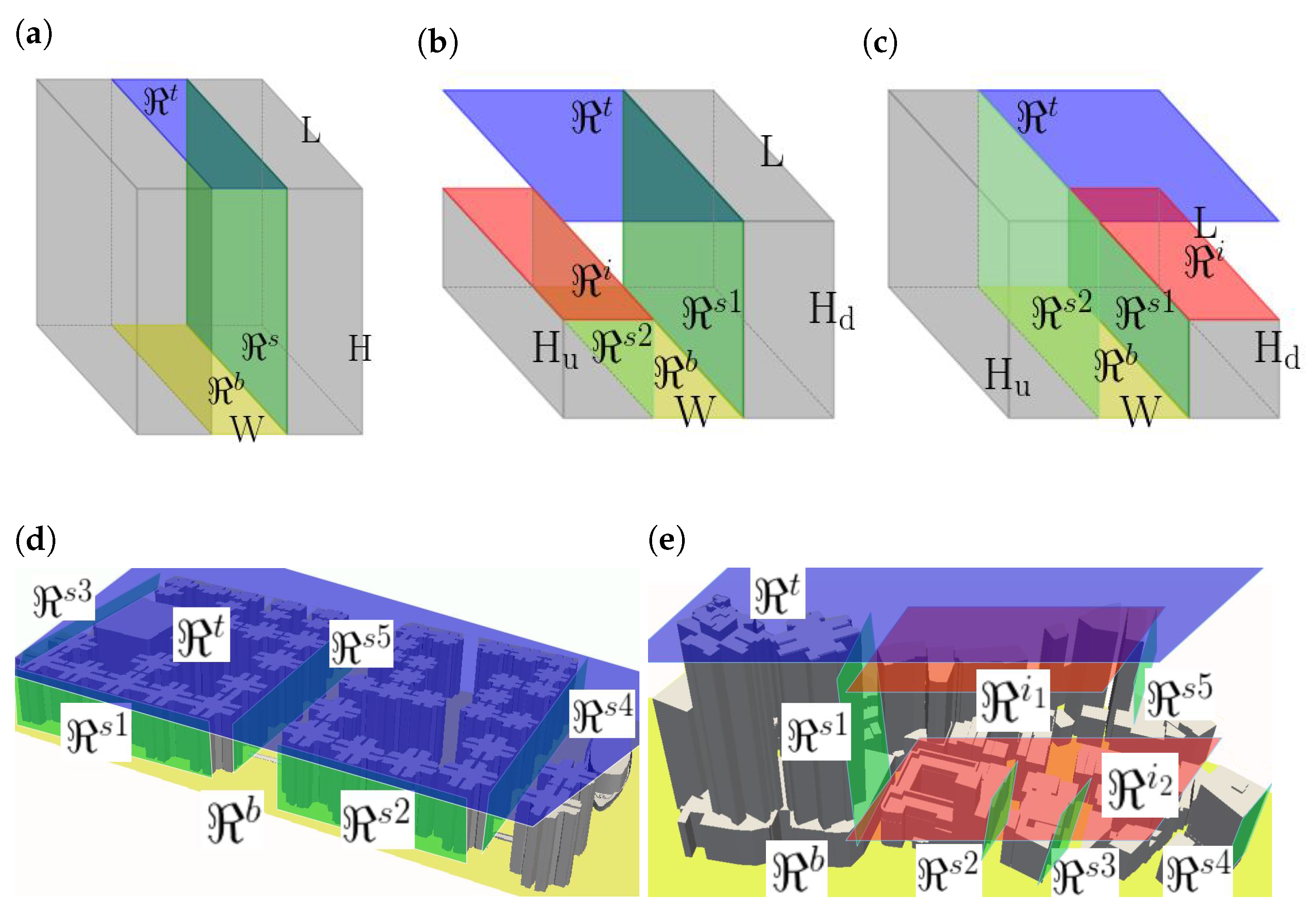
- Definition of the vortex sheets. Since strong velocity gradients occur near solid walls with no-slip boundary conditions, vorticity components are strongly localised near them. The vorticity field is, therefore, decomposed into a set of fixed, uniform vortex sheets located at the top (, the highest building height), bottom (, street level) or side () walls; for uneven geometries, intermediate vortex sheets () may be located on top of buildings. Figure 1 shows schematic illustrations of the vortex sheets for the domains considered in this study. In theory, all three vorticity components may be included for each vortex sheet; however, the predictive value of the method is lower if more basis functions are included as more calibration data are required. A subset of vorticity components and vortex sheets is, therefore, considered for the cases analysed in Section 3. Hereafter, the shorthand term ‘vorticity sheet’ refers to the combination of a vortex sheet location and vorticity component.
- Solution of Poisson equation. Velocity basis functions, , are obtained for vortex sheet j with vorticity component and unit vorticity magnitude by solving a three-dimensional Poisson Equation (A4) and horizontally averaging the Green’s function (or numerical solution). The Green’s function encapsulates the effect of the building geometry on the flow induced by a specific vorticity sheet. The Poisson equation is solved using a geometric-algebraic multi-grid solver and a free-slip boundary condition on solid surfaces; the boundary conditions are otherwise identical to the CFD model (Section 2.2), as is the computational mesh (Section 2.3).
- Synthesis. Mean wind profiles in the canyon interior are obtained by linear superposition, i.e., by summing over vortex sheets and vorticity components:where and the may be interpreted as weights that represent the strength of each vorticity sheet. The angle brackets denote the horizontal (fluid-only) average over the computational domain. The entire set of vorticity sheets (i.e., three vorticity components at each solid surface) could be included; however, this necessitates additional training data (see the calibration step below). To avoid the possibility of overdetermining or biasing the results, reduced sets are considered. They can be determined through an objective procedure (see Appendix B).
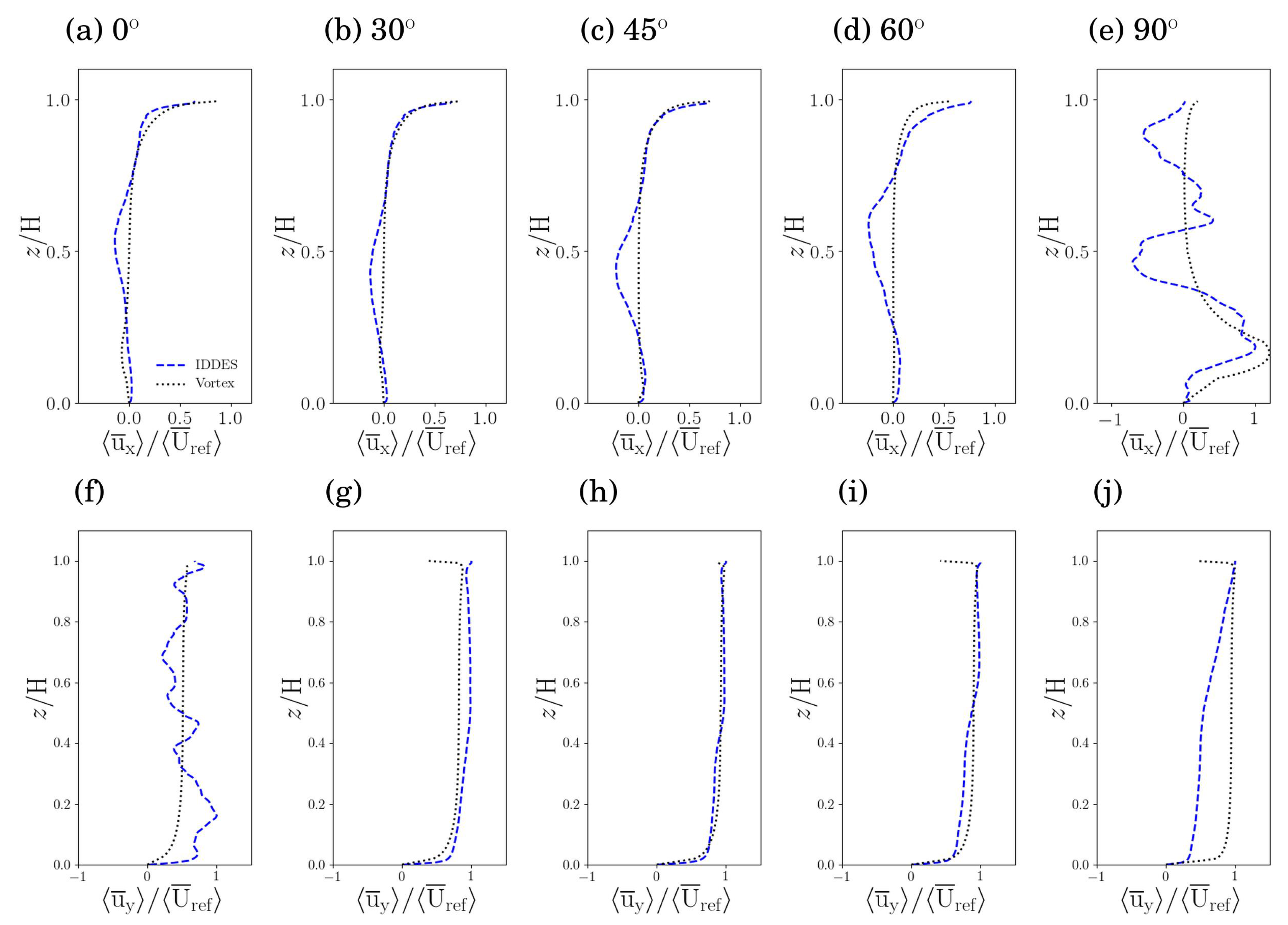
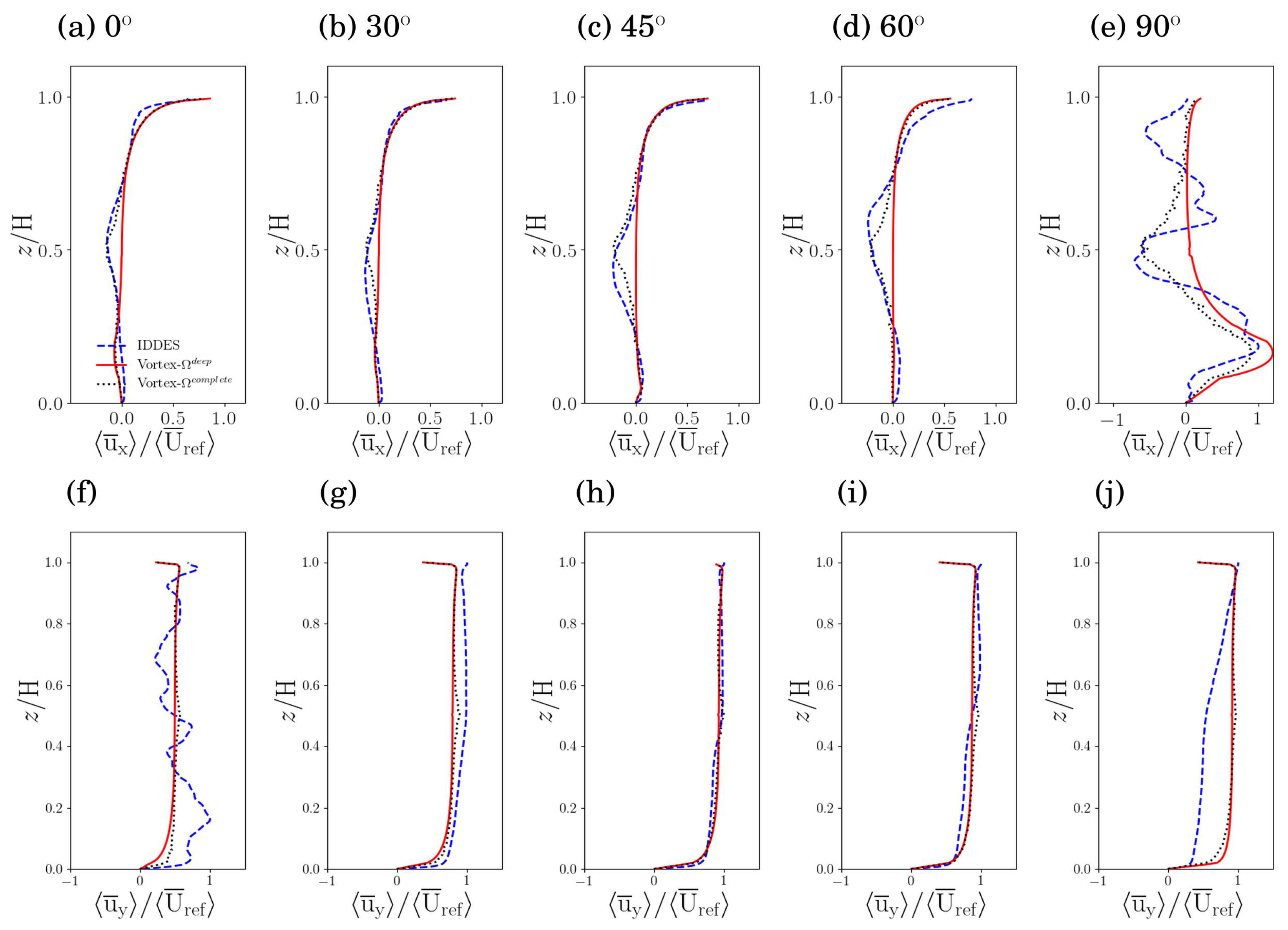
- Calibration. The weights are obtained by calibrating the basis functions against reference velocity data. The are taken to be proportional to the strength of each vorticity sheet, i.e.,where is the circulation of the vorticity sheet. Assuming that the structure of the vorticity sheets is unchanged with the wind direction, , the depends on the geometry only, i.e., they are essentially geometric constants; this assumption may be tested by applying the to other wind directions. Minimising the residual between the true profile, , and the estimated profile at a specific ,yields the geometric constants. The integral is taken over the interval, , where lies above the viscous boundary layer at the bottom, and is the (mean) canopy height. Unless otherwise stated, the geometric constants correspond to the wind direction °. The local tangential velocity, , is used to calculate . Note that but not is a function of .
- Matching. Since inviscid vortex dynamics are assumed, the interior vortex solution must be matched to the no-slip boundary condition at the ground. A logarithmic profile is introduced between the ground and the top of the log layer, i.e., , by defining the friction velocity from the log-law prediction. By construction, the log profile exerts no influence on the predicted profile in the interior, . For typical urban canyons, the streamwise velocity profile is not logarithmic near the ground: the log profile is chosen simply for convenience.
2.2. CFD Configurations
2.3. Computational Domains
2.4. Validation
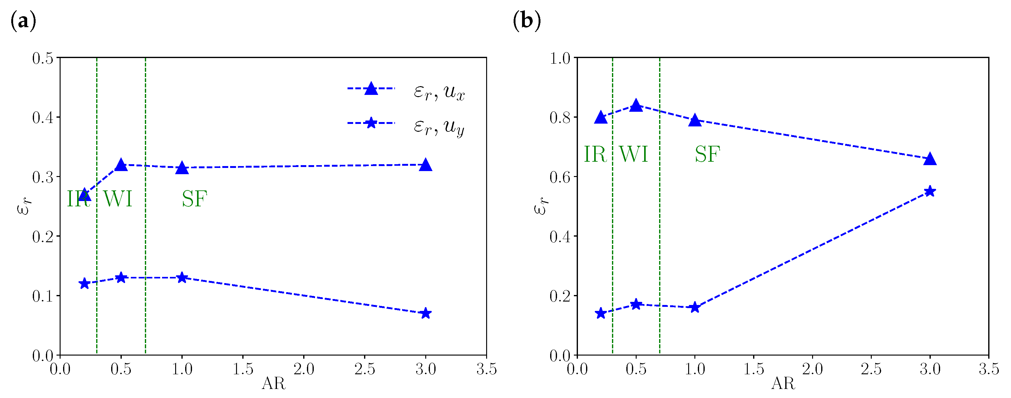
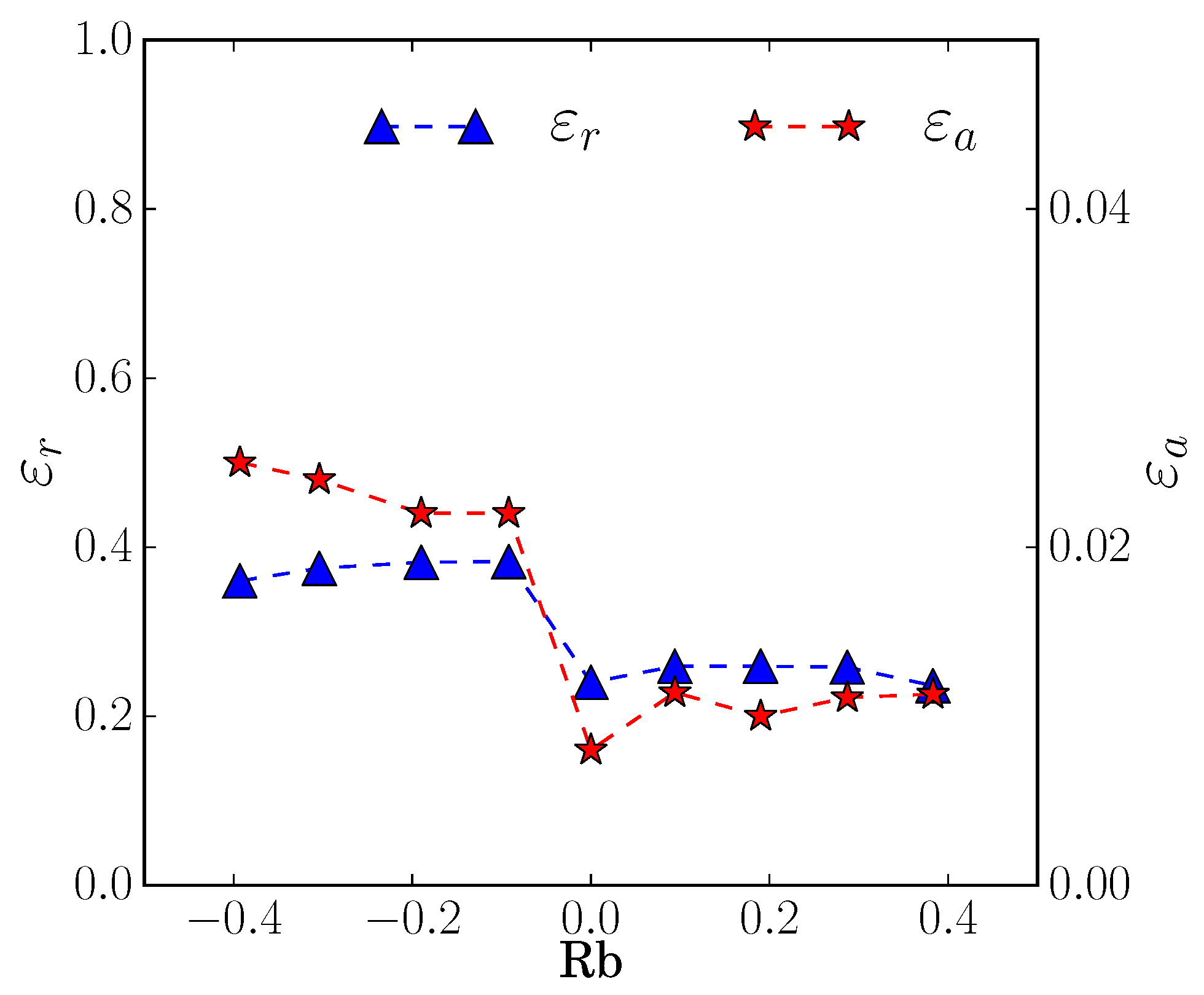
2.5. Errors
3. Geometric Effects
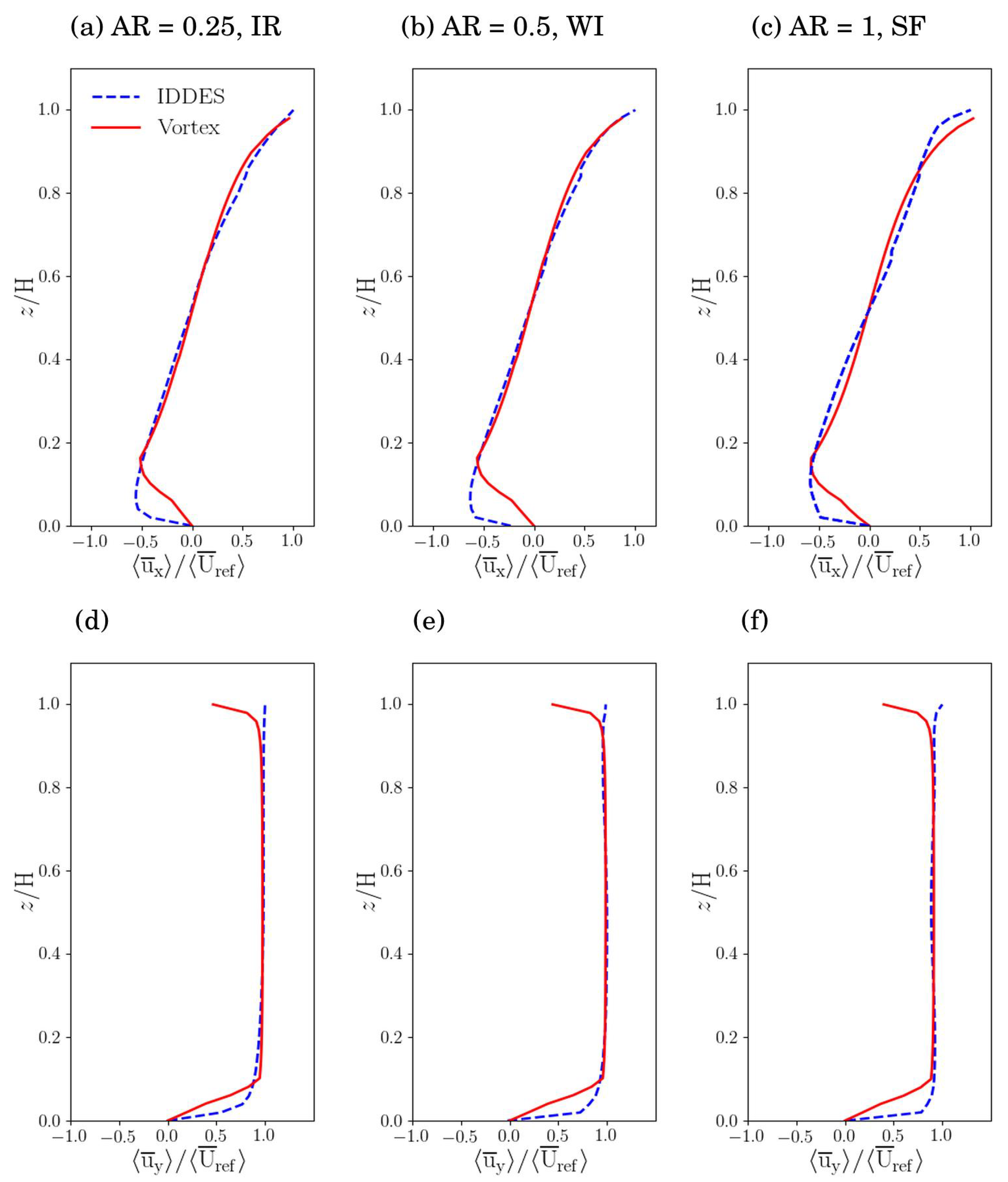
3.1. Shallow Canyons
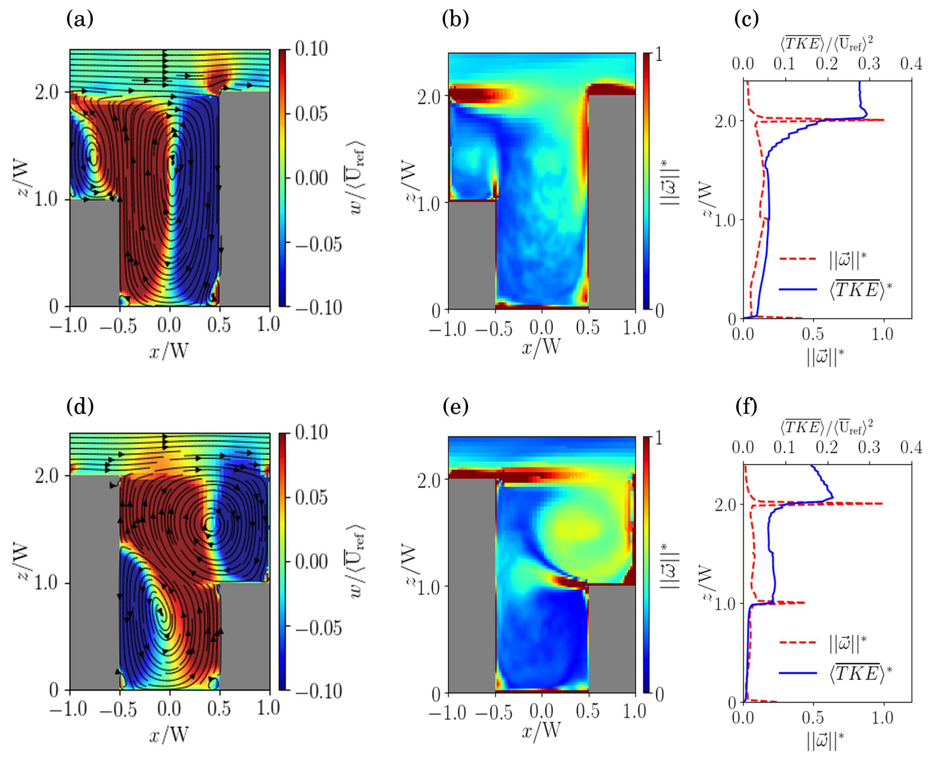
3.2. Deep Canyons
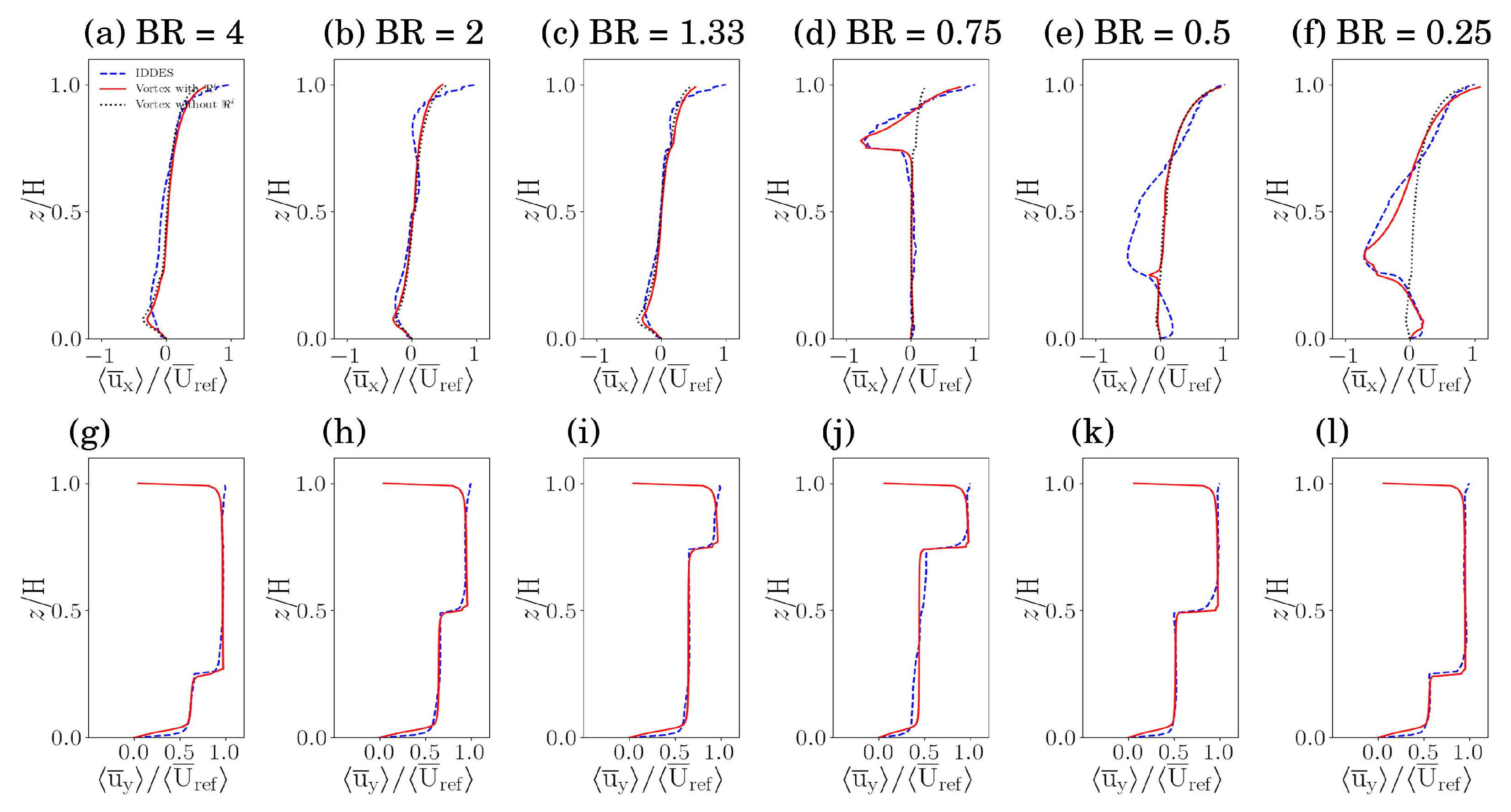
3.3. Asymmetric Canyons
3.4. Real Urban Areas
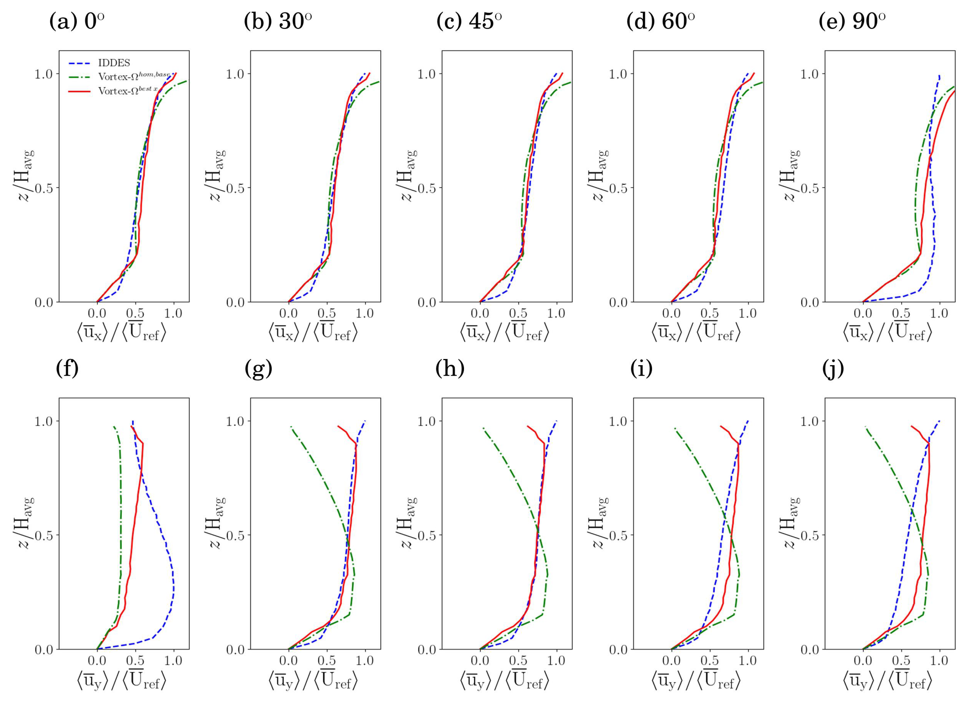
3.4.1. Homogeneous Neighbourhood
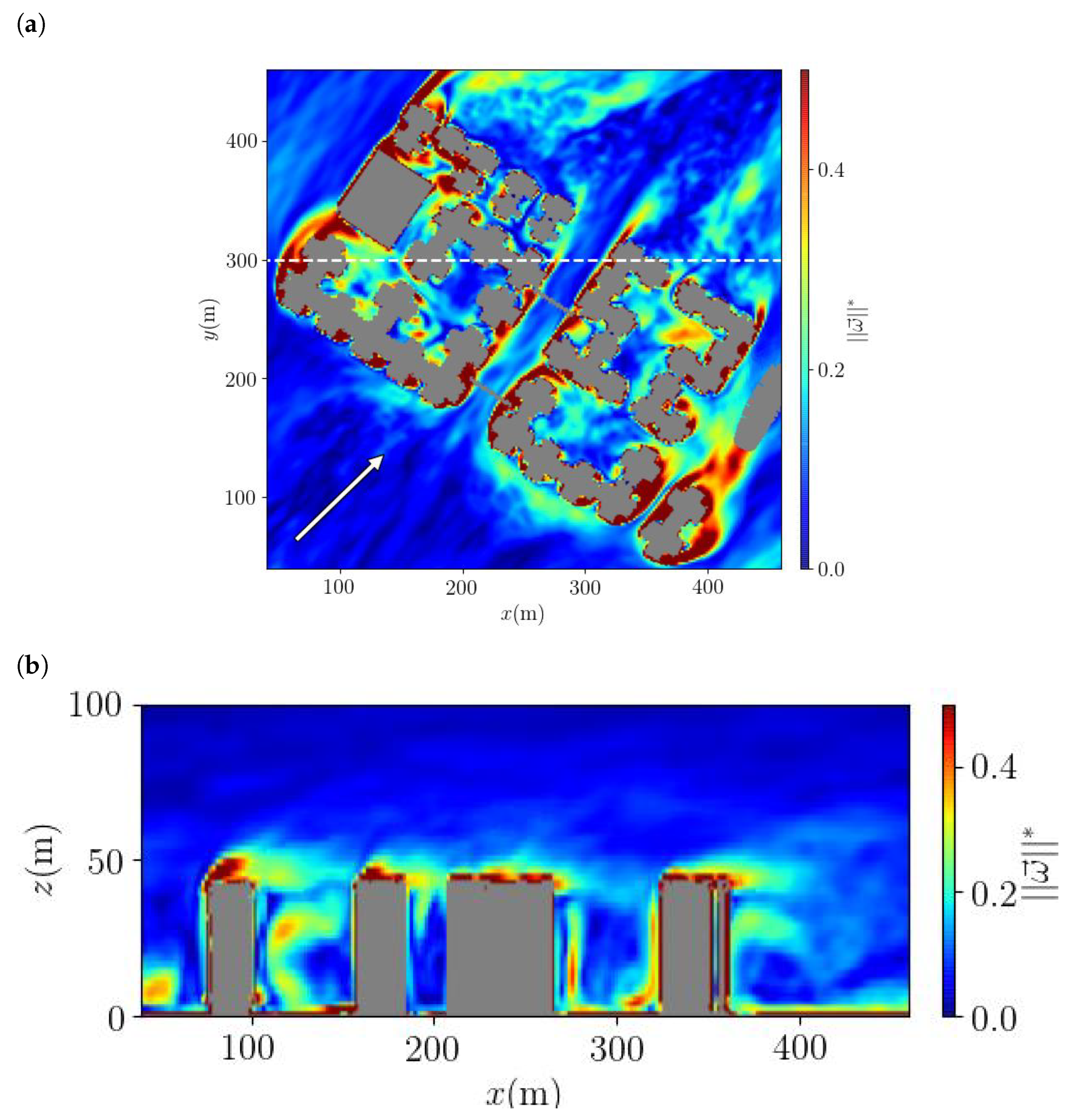
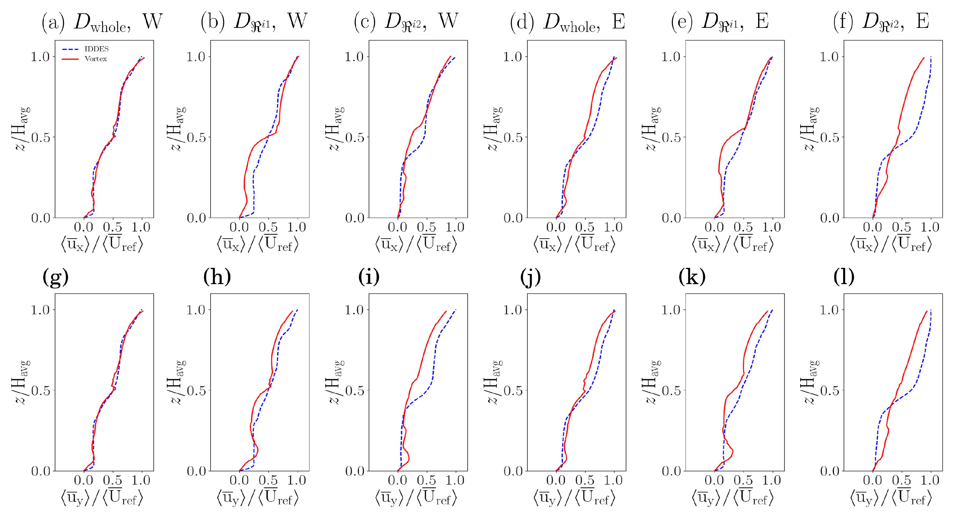
3.4.2. Heterogeneous Neighbourhood
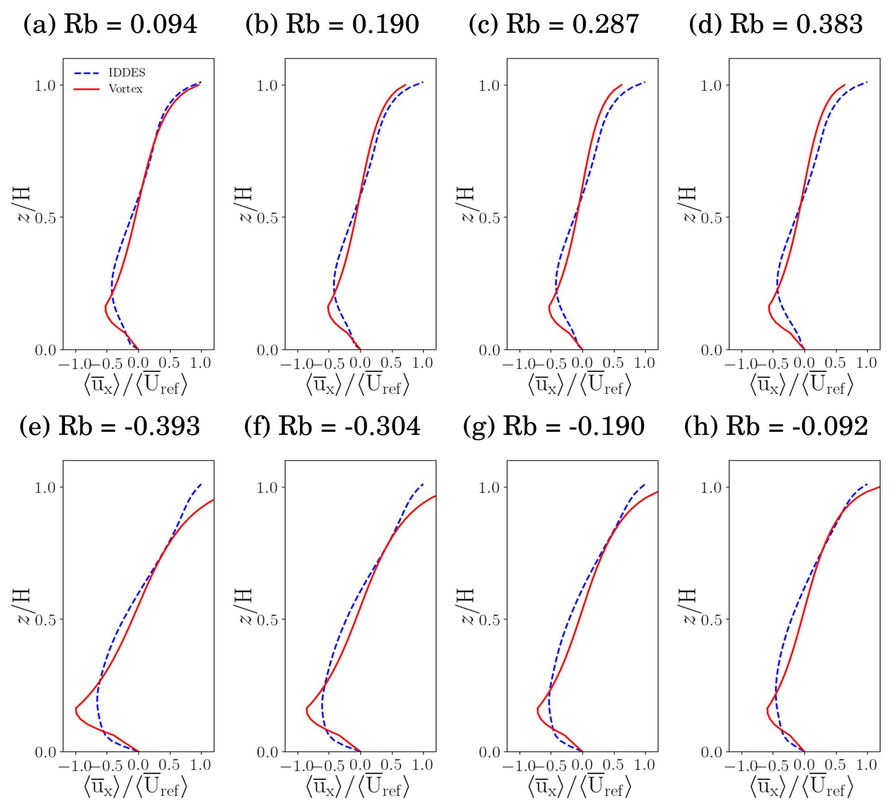
4. Stratification
5. Discussion
6. Conclusions
Author Contributions
Funding
Institutional Review Board Statement
Informed Consent Statement
Data Availability Statement
Conflicts of Interest
Appendix A. Vortex Dynamics and Vortex Method
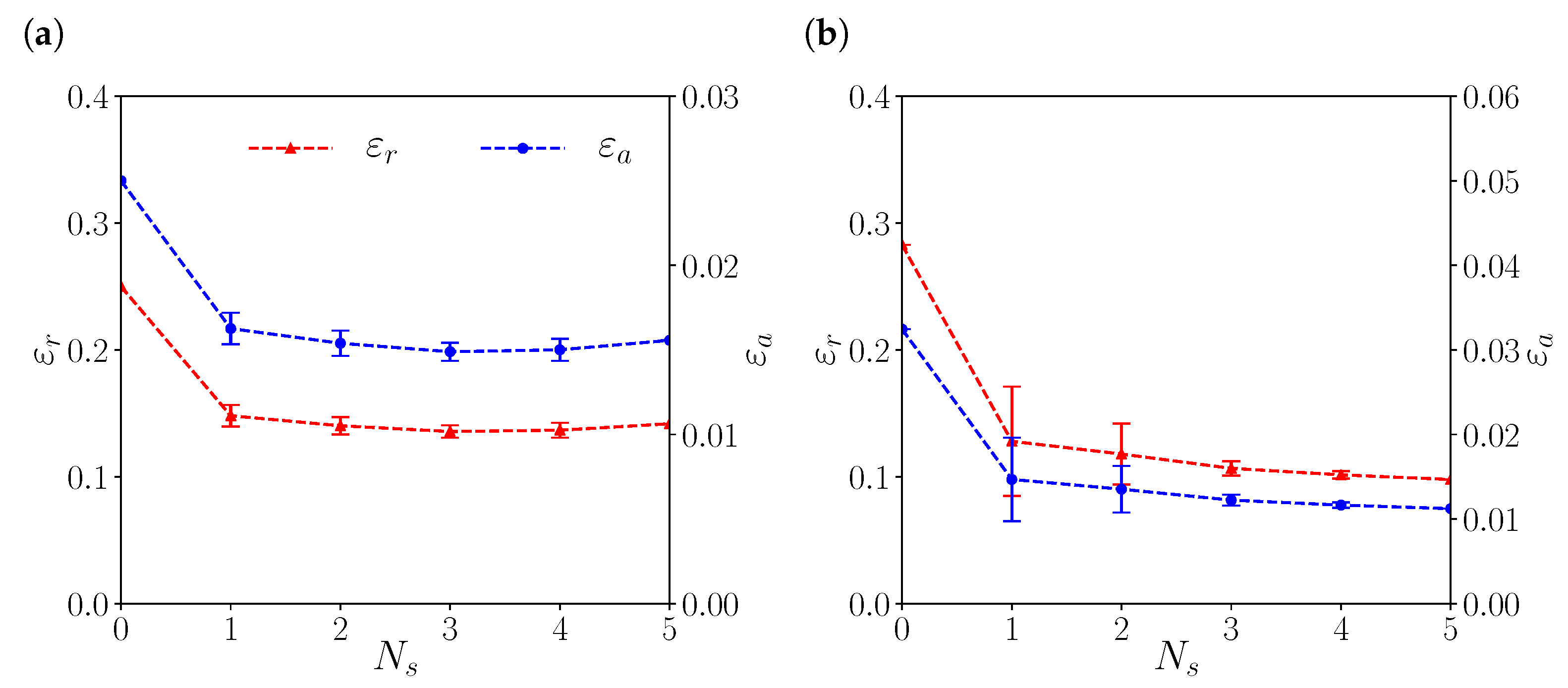
Appendix B. Selecting a Reduced Set of Vorticity Sheets

| Ground level | |||
| Roof level | |||
| Side wall | |||
| 0° | 30° | 45° | 60° | 90° | |
|---|---|---|---|---|---|
| 0.069 | 0.072 | 0.140 | 0.209 | 0.084 | |
| 0.0085 | 0.0041 | 0.0019 | 0.0028 | 0.0034 |

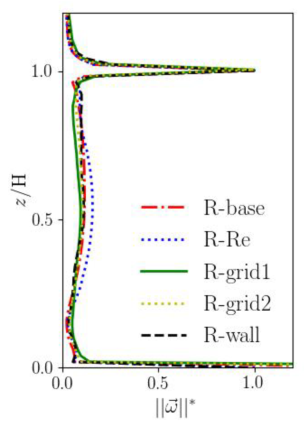
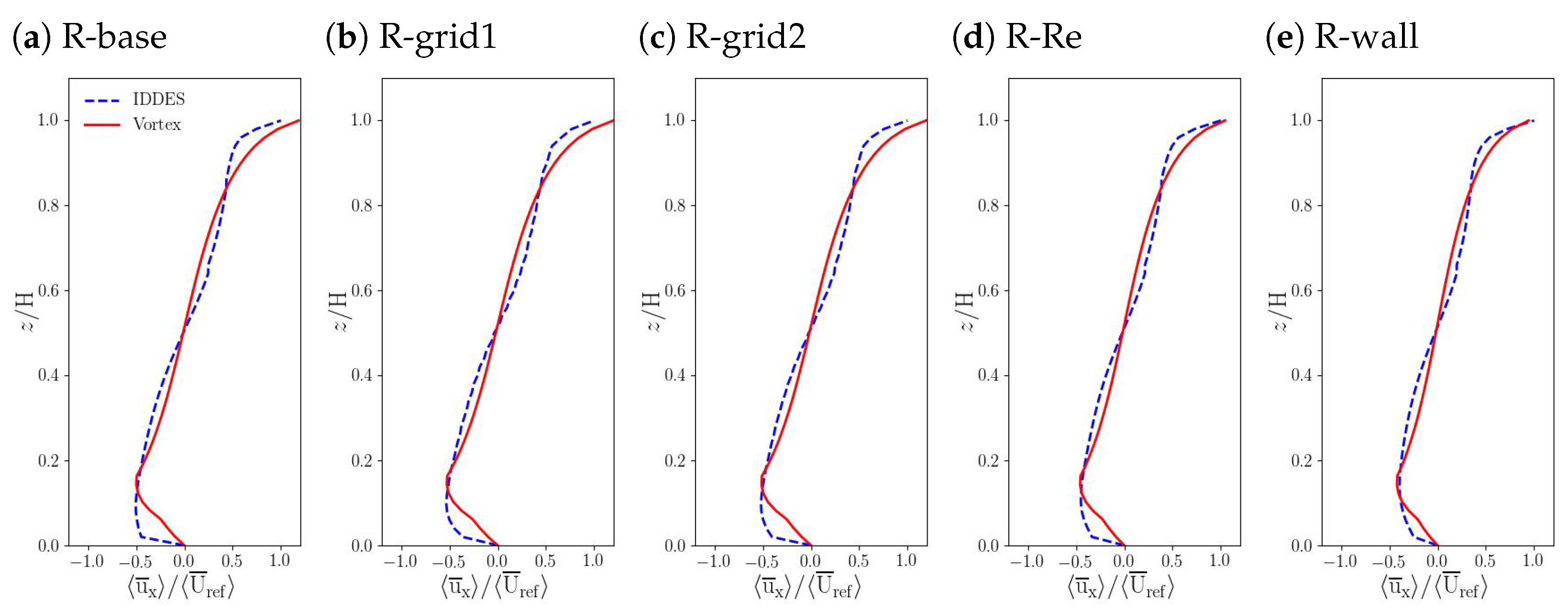
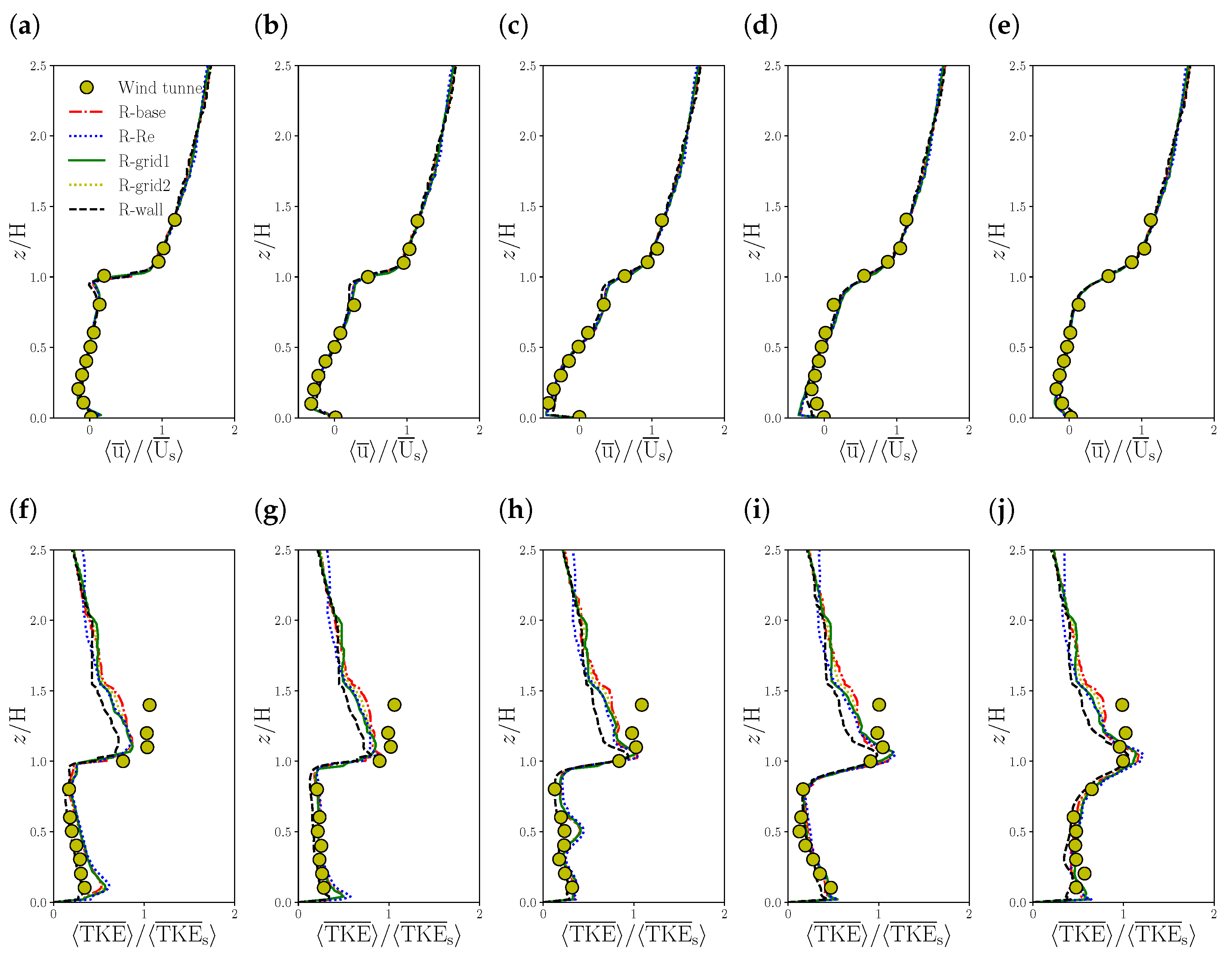
Appendix C. Sensitivity to Meshing and Wall Function
| Run | Resolution Δ | Mesh Size in the Vicinity of a Wall | Wall Function | |
|---|---|---|---|---|
| R-base | 1.0 m × 1.0 m × 1.0 m | 0.5 m × 0.5 m × 0.5 m | nutUSpaldingWallFunction | 3 |
| R-grid1 | 0.5 m × 0.5 m × 0.5 m | 0.25 m × 0.25 m × 0.25 m | nutUSpaldingWallFunction | 3 |
| R-grid2 | 1.0 m × 1.0 m × 1.0 m | 0.25 m × 0.25 m × 0.25 m | nutUSpaldingWallFunction | 3 |
| R-Re | 1.0 m × 1.0 m × 1.0 m | 0.5 m × 0.5 m × 0.5 m | nutUSpaldingWallFunction | 10 |
| R-wall | 1.0 m × 1.0 m × 1.0 m | 0.5 m × 0.5 m × 0.5 m | nutkWallFunction | 3 |


| Vortex Sheet | Velocity Component | R-Base | R-Grid1 | R-Grid2 | R-Re | R-Wall |
|---|---|---|---|---|---|---|
| () | 1.0 | 1.0 | 1.0 | 1.0 | 1.0 | |
| 0.50 | 0.53 | 0.51 | 0.45 | 0.42 | ||
| 0.15 | 0.13 | 0.14 | 0.15 | 0.18 |

| R-Base | R-Grid1 | R-Grid2 | R-Re | R-Wall | ||
|---|---|---|---|---|---|---|
| 0.018 | 0.016 | 0.017 | 0.015 | 0.012 | ||
| 0.35 | 0.32 | 0.33 | 0.32 | 0.31 |
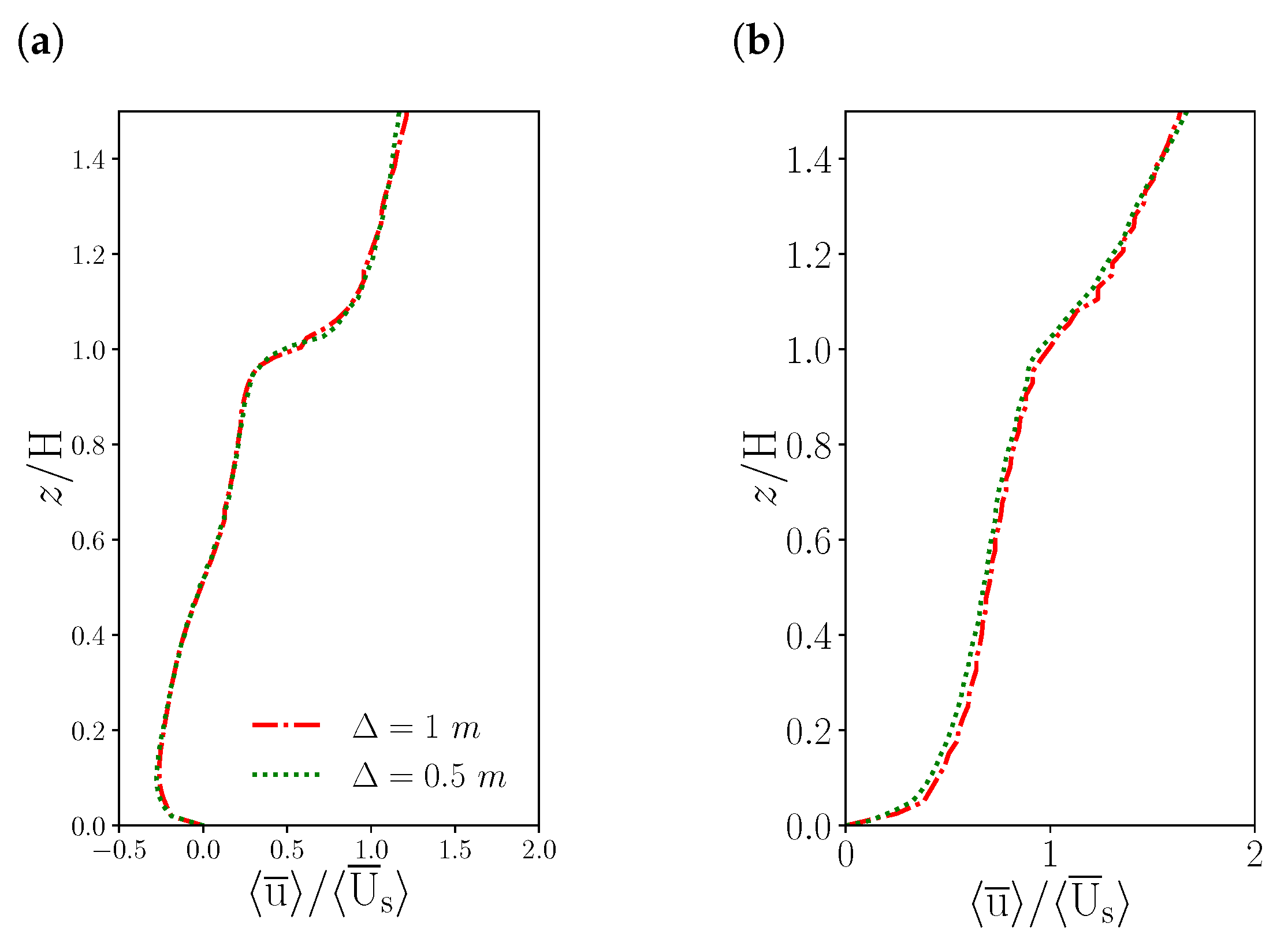
Appendix D. Grid Convergence

Appendix E. Supplementary Figures


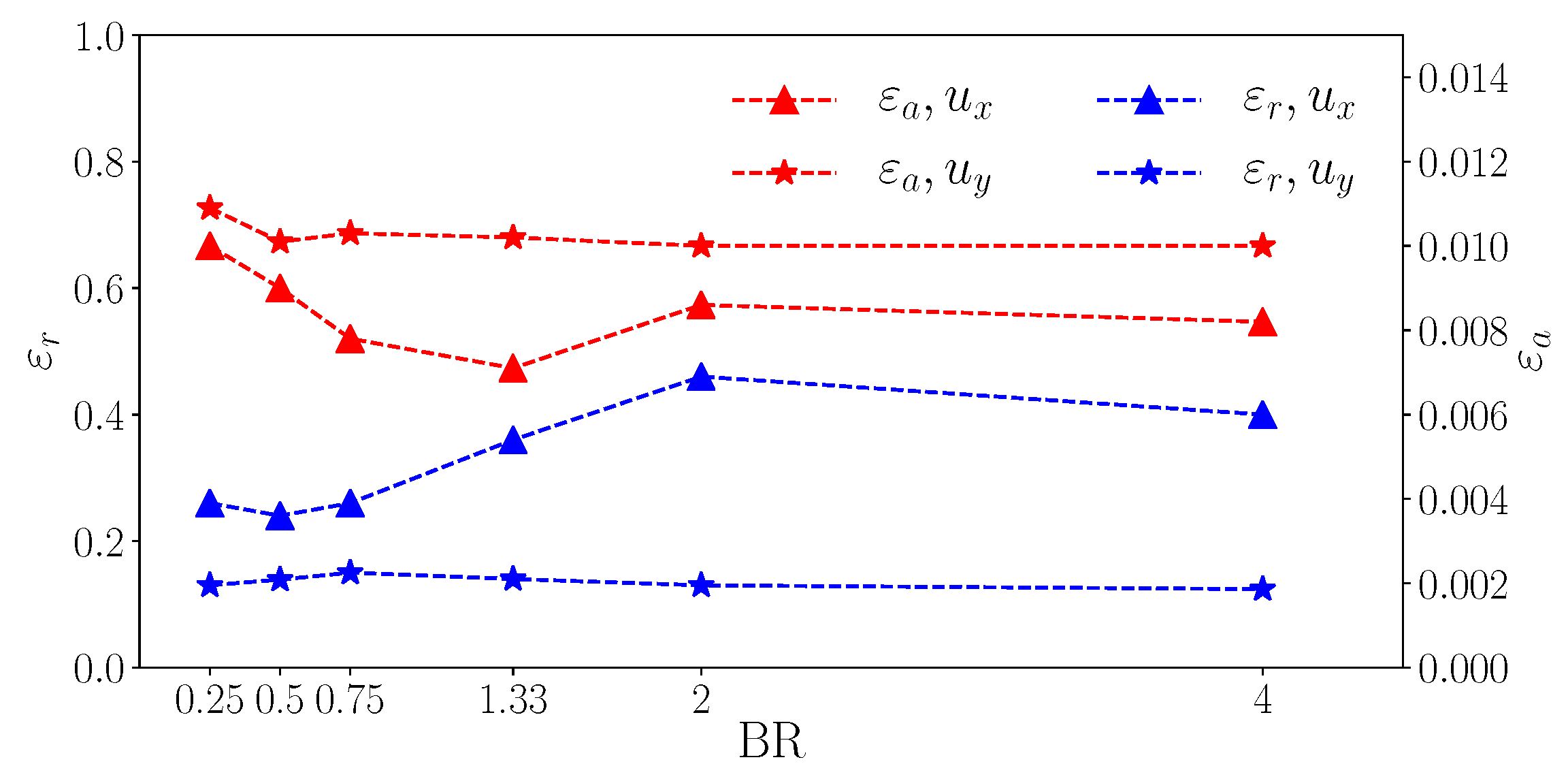
Appendix F. Errors for the Different Computational Domains
| 0° | 30° | 45° | 60° | 90° | ||
|---|---|---|---|---|---|---|
| 0.0042 | 0.0033 | 0.0038 | 0.0061 | 0.027 | ||
| 0.0044 | 0.0034 | 0.0039 | 0.0062 | 0.028 | ||
| 0.48 | 0.35 | 0.32 | 0.42 | 0.66 | ||
| 0.47 | 0.35 | 0.32 | 0.42 | 0.66 | ||
| 0.019 | 0.010 | 0.0041 | 0.008 | 0.028 | ||
| 0.019 | 0.010 | 0.0035 | 0.008 | 0.029 | ||
| 0.41 | 0.15 | 0.056 | 0.10 | 0.53 | ||
| 0.39 | 0.13 | 0.05 | 0.10 | 0.54 |
| 0° | 30° | 45° | 60° | 90° | Average | |||
|---|---|---|---|---|---|---|---|---|
| Whampoa | 0.024 | 0.024 | 0.025 | 0.025 | 0.043 | 0.028 | ||
| 0.280 | 0.260 | 0.252 | 0.240 | 0.308 | 0.268 | |||
| 0.065 | 0.012 | 0.013 | 0.019 | 0.027 | 0.027 | |||
| 0.529 | 0.110 | 0.112 | 0.189 | 0.291 | 0.246 |
| Central | 0.003 | 0.012 | 0.008 | 0.009 | 0.011 | 0.022 | ||
| 0.052 | 0.209 | 0.203 | 0.163 | 0.201 | 0.342 | |||
| 0.003 | 0.009 | 0.016 | 0.009 | 0.013 | 0.017 | |||
| 0.059 | 0.165 | 0.324 | 0.161 | 0.239 | 0.274 |
References
- Richards, P.J.; Hoxey, R.P. Appropriate boundary conditions for computational wind engineering models using the k-ϵ turbulence model. J. Wind. Eng. Ind. Aerodyn. 1993, 46–47, 145–153. [Google Scholar] [CrossRef]
- Richards, P.J.; Norris, S.E. Appropriate boundary conditions for computational wind engineering models revisited. J. Wind. Eng. Ind. Aerodyn. 2011, 99, 257–266. [Google Scholar] [CrossRef]
- Wang, K.; Stathopoulos, T. Exposure model for wind loading of buildings. J. Wind. Eng. Ind. Aerodyn. 2007, 95, 1511–1525. [Google Scholar] [CrossRef]
- Stockie, J.M. The mathematics of atmospheric dispersion modeling. SIAM Rev. 2011, 53, 349–372. [Google Scholar] [CrossRef]
- Berkowicz, R. OSPM-A parameterised street pollution model. Environ. Monit. Assess. 2000, 65, 323–331. [Google Scholar] [CrossRef]
- Soulhac, L.; Salizzoni, P.; Cierco, F.X.; Perkins, R. The model SIRANE for atmospheric urban pollutant dispersion; part i, presentation of the model. Atmos. Environ. 2011, 45, 7379–7395. [Google Scholar] [CrossRef]
- Chen, F.; Kusaka, H.; Bornstein, R.; Ching, J.; Grimmond, C.S.; Grossman-Clarke, S.; Loridan, T.; Manning, K.W.; Martilli, A.; Miao, S.; et al. The integrated WRF/urban modelling system: Development, evaluation, and applications to urban environmental problems. Int. J. Climatol. 2011, 31, 273–288. [Google Scholar] [CrossRef]
- Foken, T.; Napo, C.J. Micrometeorology, 2nd ed.; Springer: Berlin, Germany, 2008. [Google Scholar]
- Cionco, R.M. A mathematical model for air flow in a vegetative canopy. J. Appl. Meteorol. Climatol. 1965, 4, 517–522. [Google Scholar] [CrossRef]
- Barlow, J.F. Progress in observing and modelling the urban boundary layer. Urban Clim. 2014, 10, 216–240. [Google Scholar] [CrossRef] [Green Version]
- Macdonald, R.W. Modelling the mean velocity profile in the urban canopy layer. Bound.-Layer Meteorol. 2000, 97, 25–45. [Google Scholar] [CrossRef]
- Zajic, D.; Fernando, H.J.; Brown, M.J.; Pardyjak, E.R. On flows in simulated urban canopies. Environ. Fluid Mech. 2015, 15, 275–303. [Google Scholar] [CrossRef]
- Castro, I.P. Are urban-canopy velocity profiles exponential? Bound.-Layer Meteorol. 2017, 164, 337. [Google Scholar] [CrossRef]
- Di Sabatino, S.; Solazzo, E.; Paradisi, P.; Britter, R. A simple model for spatially-averaged wind profiles within and above an urban canopy. Bound.-Layer Meteorol. 2008, 127, 131–151. [Google Scholar] [CrossRef]
- Ho, Y.K.; Liu, C.H. A wind tunnel study of flows over idealised urban surfaces with roughness sublayer corrections. Theor. Appl. Climatol. 2016, 130, 305–320. [Google Scholar] [CrossRef]
- Duan, G.; Ngan, K. Effects of time-dependent inflow perturbations on turbulent flow in a street canyon. Bound.-Layer Meteorol. 2018, 167, 257–284. [Google Scholar] [CrossRef]
- Vita, G.; Salvadori, S.; Misul, D.A.; Hemida, H. Effects of inflow condition on rans and les predictions of the flow around a high-rise building. Fluids 2020, 5, 233. [Google Scholar] [CrossRef]
- Furtak-Cole, E.; Ngan, K. Predicting mean velocity profiles inside urban canyons. J. Wind. Eng. Ind. Aerodyn. 2020, 207, 104280. [Google Scholar] [CrossRef]
- Saffman, P.G. Vortex Dynamics; Cambridge University Press: Cambridge, UK, 1992. [Google Scholar]
- Wu, J.Z.; Ma, H.Y.; Zhou, M.D. Vorticity and Vortex Dynamics; Springer: Berlin, Germany, 2007. [Google Scholar]
- Ngan, K.; Lo, K.W. Revisiting the flow regimes for urban street canyons using the numerical Green’s function. Environ. Fluid Mech. 2016, 16, 313–334. [Google Scholar] [CrossRef]
- Wang, H.; Brimblecombe, P.; Ngan, K. Particulate matter inside and around elevated walkways. Sci. Total Environ. 2020, 699, 134256. [Google Scholar] [CrossRef]
- Yao, L.; Liu, C.H.; Mo, Z.; Cheng, W.C.; Brasseur, G.P.; Chao, C.Y. Statistical analysis of the organized turbulence structure in the inertial and roughness sublayers over real urban area by building-resolved large-eddy simulation. Build. Environ. 2022, 207, 108464. [Google Scholar] [CrossRef]
- Li, X.X.; Liu, C.H.; Leung, D.Y.; Lam, K.M. Recent progress in CFD modelling of wind field and pollutant transport in street canyons. Atmos. Environ. 2006, 40, 5640–5658. [Google Scholar] [CrossRef]
- Lin, Y.; Hang, J.; Yang, H.; Chen, L.; Chen, G.; Ling, H.; Sandberg, M.; Claesson, L.; Lam, C.K. Investigation of the Reynolds number independence of cavity flow in 2d street canyons by wind tunnel experiments and numerical simulations. Build. Environ. 2021, 201, 107965. [Google Scholar] [CrossRef]
- Aboelata, A.; Sodoudi, S. Evaluating urban vegetation scenarios to mitigate urban heat island and reduce buildings’ energy in dense built-up areas in Cairo. Build. Environ. 2019, 166, 106407. [Google Scholar] [CrossRef]
- Ulpiani, G. On the linkage between urban heat island and urban pollution island: Three-decade literature review towards a conceptual framework. Sci. Total Environ. 2021, 751, 141727. [Google Scholar] [CrossRef] [PubMed]
- Fan, Y.; Hunt, J.; Wang, Q.; Yin, S.; Li, Y. Water tank modelling of variations in inversion breakup over a circular city. Build. Environ. 2019, 164, 106342. [Google Scholar] [CrossRef]
- Zhou, X.; Ying, A.; Cong, B.; Kikumoto, H.; Ooka, R.; Kang, L.; Hu, H. Large eddy simulation of the effect of unstable thermal stratification on airflow and pollutant dispersion around a rectangular building. J. Wind. Eng. Ind. Aerodyn. 2021, 211, 104526. [Google Scholar] [CrossRef]
- Pullin, D.I. Contour dynamics methods. Annu. Rev. Fluid Mech. 1992, 24, 89–115. [Google Scholar] [CrossRef]
- Flierl, G.R. Isolated eddy models in geophysics. Annu. Rev. Fluid Mech. 1987, 19, 493–550. [Google Scholar] [CrossRef]
- Ngan, K.; Lo, K.W. Linear error dynamics for turbulent flow in urban street canyons. J. Appl. Meteorol. Climatol. 2017, 56, 1195–1208. [Google Scholar] [CrossRef]
- Louka, P.; Belcher, S.E.; Harrison, R.G. Coupling between air flow in streets and the well-developed boundary layer aloft. Atmos. Environ. 2000, 34, 2613–2621. [Google Scholar] [CrossRef]
- Guillas, S.; Glover, N.; Malki-Epshtein, L. Bayesian calibration of the constants of the k–ε turbulence model for a CFD model of street canyon flow. Comput. Methods Appl. Mech. Eng. 2014, 279, 536–553. [Google Scholar] [CrossRef] [Green Version]
- Weerasuriya, A.U.; Zhang, X.; Lu, B.; Tse, K.T.; Liu, C.H. Optimizing lift-up design to maximize pedestrian wind and thermal comfort in hot-calm and cold-windy climates. Sustain. Cities Soc. 2020, 58, 102146. [Google Scholar] [CrossRef]
- Weerasuriya, A.U.; Zhang, X.; Lu, B.; Tse, K.T.; Liu, C.H. A Gaussian process-based emulator for modeling pedestrian-level wind field. Build. Environ. 2021, 188, 107500. [Google Scholar] [CrossRef]
- Pope, S.B. Turbulent Flows; Cambridge University Press: Cambridge, UK, 2000. [Google Scholar]
- Weller, H.G.; Tabor, G.; Jasak, H.; Fureby, C. A tensorial approach to computational continuum mechanics using object-oriented techniques. Comput. Phys. 1998, 12, 620–631. [Google Scholar] [CrossRef]
- Darwish, M.; Moukalled, F. The Finite Volume Method in Computational Fluid Dynamics; Springer: Berlin, Germany, 2016. [Google Scholar]
- Shur, M.L.; Spalart, P.R.; Strelets, M.K.; Travin, A.K. A hybrid RANS-LES approach with delayed-DES and wall-modelled LES capabilities. Int. J. Heat Fluid Flow 2008, 29, 1638–1649. [Google Scholar] [CrossRef]
- Tominaga, Y.; Stathopoulos, T. CFD modeling of pollution dispersion in a street canyon: Comparison between LES and RANS. J. Wind Eng. Ind. Aerodyn. 2011, 99, 340–348. [Google Scholar] [CrossRef] [Green Version]
- Spalding, D.B. A single formula for the law of the wall. Appl. Mech. 1961, 28, 455. [Google Scholar] [CrossRef]
- Maronga, B.; Gryschka, M.; Heinze, R.; Hoffmann, F.; Kanani-Sühring, F.; Keck, M.; Ketelsen, K.; Letzel, M.O.; Sühring, M.; Raasch, S. The parallelized large-eddy simulation model (PALM) version 4.0 for atmospheric and oceanic flows: Model formulation, recent developments, and future perspectives. Geosci. Model Dev. 2015, 8, 2515–2551. [Google Scholar] [CrossRef] [Green Version]
- Moeng, C.H.; Wyngaard, J.C. Spectral analysis of large-eddy simulations of the convective boundary layer. J. Atmos. Sci. 1988, 45, 3573–3587. [Google Scholar] [CrossRef]
- Saiki, E.M.; Moeng, C.H.; Sullivan, P.P. Large-eddy simulation of the stably stratified planetary boundary layer. Bound.-Layer Meteorol. 2000, 95, 1–30. [Google Scholar] [CrossRef]
- Castillo, M.C.; Inagaki, A.; Kanda, M. The effects of inner-and outer-layer turbulence in a convective boundary layer on the near-neutral inertial sublayer over an urban-like surface. Bound.-Layer Meteorol. 2011, 140, 453–469. [Google Scholar] [CrossRef]
- Inagaki, A.; Castillo, M.C.; Yamashita, Y.; Kanda, M.; Takimoto, H. Large-eddy simulation of coherent flow structures within a cubical canopy. Bound.-Layer Meteorol. 2012, 142, 207–222. [Google Scholar] [CrossRef]
- Han, B.S.; Baik, J.J.; Park, S.B.; Kwak, K.H. Large-eddy simulations of reactive pollutant dispersion in the convective boundary layer over flat and urban-like surfaces. Bound.-Layer Meteorol. 2019, 172, 271–289. [Google Scholar] [CrossRef]
- Gronemeier, T.; Raasch, S.; Ng, E. Effects of unstable stratification on ventilation in Hong Kong. Atmosphere 2017, 8, 168. [Google Scholar] [CrossRef] [Green Version]
- Wang, H.; Ngan, K. Effects of inhomogeneous ground-level pollutant sources under different wind directions. Environ. Pollut. 2021, 289, 117903. [Google Scholar] [CrossRef] [PubMed]
- Kim, J.J.; Baik, J.J. Urban street-canyon flows with bottom heating. Atmos. Environ. 2001, 35, 3395–3404. [Google Scholar] [CrossRef]
- Cheng, W.C.; Liu, C.H. Large-eddy simulation of flow and pollutant transports in and above two-dimensional idealized street canyons. Bound.-Layer Meteorol. 2011, 139, 411–437. [Google Scholar] [CrossRef] [Green Version]
- Li, X.X.; Britter, R.; Norford, L.K. Effect of stable stratification on dispersion within urban street canyons: A large-eddy simulation. Atmos. Environ. 2016, 144, 47–59. [Google Scholar] [CrossRef] [Green Version]
- Lawson, R.E., Jr.; Lee, R.L. Mean flow and turbulence measurements around a 2-D array of buildings in a wind tunnel. In Proceedings of the 11th Joint AMS/AWMA Conference on the Applications of Air Pollution Meteorology, Long Beach, CA, USA, 9 January 2000. [Google Scholar]
- Duan, G.; Takemi, T. Predicting urban surface roughness aerodynamic parameters using random forest. J. Appl. Meteorol. Climatol. 2021, 60, 999–1018. [Google Scholar] [CrossRef]
- Kwak, K.H.; Baik, J.J.; Ryu, Y.H.; Lee, S.H. Urban air quality simulation in a high-rise building area using a CFD model coupled with mesoscale meteorological and chemistry-transport models. Atmos. Environ. 2015, 100, 167–177. [Google Scholar] [CrossRef]
- Chang, J.C.; Hanna, S.R. Air quality model performance evaluation. Meteorol. Atmos. Phys. 2004, 87, 167–196. [Google Scholar] [CrossRef]
- Uehara, K.; Murakami, S.; Oikawa, S.; Wakamatsu, S. Wind tunnel experiments on how thermal stratification affects flow in and above urban street canyons. Atmos. Environ. 2000, 34, 1553–1562. [Google Scholar] [CrossRef]
- Oke, T.R. Street design and urban canopy layer climate. Energy Build. 1988, 11, 103–113. [Google Scholar] [CrossRef]
- Hunter, L.J.; Watson, I.D.; Johnson, G.T. Modelling air flow regimes in urban canyons. Energy Build. 1990, 15, 315–324. [Google Scholar] [CrossRef]
- He, L.; Hang, J.; Wang, X.; Lin, B.; Li, X.; Lan, G. Numerical investigations of flow and passive pollutant exposure in high-rise deep street canyons with various street aspect ratios and viaduct settings. Sci. Total Environ. 2017, 584, 189–206. [Google Scholar] [CrossRef]
- Chew, L.W.; Aliabadi, A.A.; Norford, L.K. Flows across high aspect ratio street canyons: Reynolds number independence revisited. Environ. Fluid Mech. 2018, 18, 1275–1291. [Google Scholar] [CrossRef]
- Addepalli, B.; Pardyjak, E.R. Investigation of the flow structure in step-up street canyons—Mean flow and turbulence statistics. Bound.-Layer Meteorol. 2013, 148, 133–155. [Google Scholar] [CrossRef]
- Addepalli, B.; Pardyjak, E.R. A study of flow fields in step-down street canyons. Environ. Fluid Mech. 2015, 15, 439–481. [Google Scholar] [CrossRef]
- Nazarian, N.; Kleissl, J. Realistic solar heating in urban areas: Air exchange and street-canyon ventilation. Build. Environ. 2016, 95, 75–93. [Google Scholar] [CrossRef] [Green Version]
- Wood, C.R.; Järvi, L.; Kouznetsov, R.D.; Nordbo, A.; Joffre, S.; Drebs, A.; Vihma, T.; Hirsikko, A.; Suomi, I.; Fortelius, C.; et al. An overview of the urban boundary layer atmosphere network in Helsinki. Bull. Am. Meteorol. Soc. 2013, 94, 1675–1690. [Google Scholar] [CrossRef]
- Tian, G.; Conan, B.; Calmet, I. Turbulence-kinetic-energy budget in the urban-like boundary layer using large-eddy simulation. Bound.-Layer Meteorol. 2020, 178, 201–223. [Google Scholar] [CrossRef]
- Duan, G.; Ngan, K. Sensitivity of turbulent flow around a 3-d building array to urban boundary-layer stability. J. Wind. Eng. Ind. Aerodyn. 2019, 193, 103958. [Google Scholar] [CrossRef]
- Lo, K.W.; Ngan, K. Characterising urban ventilation and exposure using Lagrangian particles. J. Appl. Meteorol. Climatol. 2017, 56, 1177–1194. [Google Scholar] [CrossRef]
- Chatzimichailidis, A.E.; Argyropoulos, C.D.; Assael, M.J.; Kakosimos, K.E. Qualitative and quantitative investigation of multiple large eddy simulation aspects for pollutant dispersion in street canyons using openfoam. Atmosphere 2019, 10, 17. [Google Scholar] [CrossRef]


| Canyon | W | H | L | Illustration | ||||
|---|---|---|---|---|---|---|---|---|
| Shallow | 0.25 | 5H | 3H | 5H | 200 m | 50 m | 150 m | Figure 1a |
| 0.5 | 3H | 3H | 5H | 100 m | 50 m | 150 m | Figure 1a | |
| Deep | 1 | 2W | 3W | 5H | 50 m | 50 m | 150 m | Figure 1a |
| 3 | 2W | 3W | 5H | 50 m | 150 m | 150 m | Figure 1a | |
| Step-up | - | 2W | 3W | 5 | 50 m | : 50 m; : 100 m | 150 m | Figure 1b |
| Step-down | - | 2W | 3W | 5 | 50 m | : 100 m; : 50 m | 150 m | Figure 1c |
| Whampoa | ∼1.4 | 480 m | 480 m | 200 m | - | : 41.4 m | - | Figure 1d |
| Central | ∼2 | 260 m | 140 m | 500 m | - | : 48 m | - | Figure 1e |
| Canyon | W | L | |||
|---|---|---|---|---|---|
| Step-up | 4 | 50 m | 25 m | 100 m | 150 m |
| 2 | 50 m | 50 m | 100 m | 150 m | |
| 1.33 | 50 m | 75 m | 100 m | 150 m | |
| Step-down | 0.75 | 50 m | 100 m | 75 m | 150 m |
| 0.5 | 50 m | 100 m | 50 m | 150 m | |
| 0.25 | 50 m | 100 m | 25 m | 150 m |
| Stratification | Stable (K) | Neutral (K) | Unstable (K) |
|---|---|---|---|
| −8, −6, −4, −2 | 0 | 2, 4, 6, 8 | |
| Rb | 0.38, 0.29, 0.19, 0.09 | 0 | −0.09, −0.19, −0.30, −0.39 |
Disclaimer/Publisher’s Note: The statements, opinions and data contained in all publications are solely those of the individual author(s) and contributor(s) and not of MDPI and/or the editor(s). MDPI and/or the editor(s) disclaim responsibility for any injury to people or property resulting from any ideas, methods, instructions or products referred to in the content. |
© 2022 by the authors. Licensee MDPI, Basel, Switzerland. This article is an open access article distributed under the terms and conditions of the Creative Commons Attribution (CC BY) license (https://creativecommons.org/licenses/by/4.0/).
Share and Cite
Wang, H.; Furtak-Cole, E.; Ngan, K. Estimating Mean Wind Profiles Inside Realistic Urban Canopies. Atmosphere 2023, 14, 50. https://doi.org/10.3390/atmos14010050
Wang H, Furtak-Cole E, Ngan K. Estimating Mean Wind Profiles Inside Realistic Urban Canopies. Atmosphere. 2023; 14(1):50. https://doi.org/10.3390/atmos14010050
Chicago/Turabian StyleWang, Huanhuan, Eden Furtak-Cole, and Keith Ngan. 2023. "Estimating Mean Wind Profiles Inside Realistic Urban Canopies" Atmosphere 14, no. 1: 50. https://doi.org/10.3390/atmos14010050