Article

Fast Models for Predicting Pollutant Dispersion inside Urban Canopies

1
Department of Mechanical Engineering, The University of Hong Kong, Pokfulam, Hong Kong, China
2
School of Energy and Environment, City University of Hong Kong, Kowloon, Hong Kong, China
3
Division of Atmospheric Sciences, Desert Research Institute, Reno, NV 89512, USA
4
Institute of Ocean and Earth Sciences, University of Malaya, Kuala Lumpur 50603, Malaysia
*
Author to whom correspondence should be addressed.
Atmosphere 2023, 14(9), 1337; https://doi.org/10.3390/atmos14091337
Submission received: 25 July 2023 / Revised: 19 August 2023 / Accepted: 21 August 2023 / Published: 24 August 2023
(This article belongs to the Special Issue Multiscale Aspects of Mesoscale and Microscale Flows)

Abstract

:
A fast pollutant dispersion model for urban canopies is developed by coupling mean wind profiles to a parameterisation of turbulent diffusion and solving the time-dependent advection–diffusion equation. The performance of a simplified, coarse-grained representation of the velocity field is investigated. Spatially averaged mean wind profiles within local averaging regions or repeating units are predicted by solving the three-dimensional Poisson equation for a set of discrete vortex sheets. For each averaging region, the turbulent diffusion is parameterised in terms of the mean wind profile using empirical constants derived from large-eddy simulation (LES). Nearly identical results are obtained whether the turbulent fluctuations are specified explicitly or an effective diffusivity is used in their place: either version of the fast dispersion model shows much better agreement with LES than does the Gaussian plume model (e.g., the normalized mean square error inside the canopy is several times smaller). Passive scalar statistics for a regular cubic building array show improved agreement with LES when wind profiles vary in the horizontal. The current implementation is around 50 times faster than LES. With its combination of computational efficiency and moderate accuracy, the fast model may be suitable for time-critical applications such as emergency dispersion modelling.

1. Introduction

Fast and accurate prediction of pollutant dispersion is important for practical applications such as operational air-quality modelling and emergency dispersion modelling. Computational fluid dynamics (CFD), which has been extensively applied to pollutant dispersion in idealised [1] and realistic [2,3] urban areas, features relatively high accuracy; however, it is too computationally demanding for time-critical applications. Hence, there is a need for a fast dispersion model that can provide useful predictions without significant computational resources, extensive training data or many adjustable parameters.
The simplest dispersion model is the Gaussian plume model (GPM) [4], which is still widely used. In the original formulation, the pollutant concentration downwind of a point source is estimated by assuming flat terrain and an eddy diffusivity that increases linearly with downwind distance [5]. The GPM is therefore not well-suited to the urban canopy layer, where pollutants are emitted and many people live and work. The intrinsic limitations of the GPM have helped spur the development of fast dispersion models that are more appropriate for urban areas. The Quick Urban & Industrial Complex (QUIC) model is based on a variational solution for a steady velocity field [6] and a Lagrangian stochastic model for the time-dependent dispersion [7]. Although QUIC has been successfully applied in a variety of contexts (e.g., [8]), accuracy is potentially limited by the initial guess for the velocity and the nonlocal mixing parameterisation. The urban dispersion models SIRANE [9] and MUNICH [10] assume constant concentration on the building scale (i.e., within a street canyon) and parameterise the mean velocity profiles and turbulent transfer. They show good agreement with in situ observations [11,12]; however, information about individual buildings is lost as only the canyon dimensions and aspect ratio are considered.
The complexity of the urban environment is such that any fast dispersion model must rely on assumptions, approximations and empirical relationships. Hence, models such as QUIC, SIRANE and MUNICH may not be well-suited to all applications or geometries. In this paper, we introduce a new fast dispersion model based on coarse graining of the velocity field, i.e., spatial averaging over subregions or repeating units. This is a potentially attractive strategy because accurate and computationally efficient models of spatial averages are more easily obtained than ones for the fine-scale turbulent velocity field. We estimate the spatially averaged mean wind profiles within the urban canopy by approximating the vorticity field [13] and couple them to different turbulence parameterisations. Although the time-dependent three-dimensional (3D) advection–diffusion equation is solved, mean wind profiles within subregions are used in place of a continuously varying 3D velocity field. For one of the parameterisations, turbulent fluctuations within each subregion are prescribed; for the other one, the associated effective diffusivity is used instead.
This study introduces a new multiscale fast dispersion model based on estimates of the spatially averaged wind profiles and applies it to the canonical case of a cubic building array. The fast dispersion model (FM) is presented in Section 2: the estimation of the mean wind profiles within the array units is reviewed and the two turbulence parameterisations are described. The methodology section details the implementation of two versions of the FM, which are distinguished by their turbulence parameterisation, as well as the LES model that is used for calibration and assessment (Section 3). The performance of the fast model is assessed in Section 4 through comparisons with LES and the GPM. The sensitivity to mean wind speeds and the specification of the diffusivity tensor is described in Section 5 and Section 6, respectively. Limitations of the fast dispersion model are discussed in Section 7. Practical implications for operational dispersion modelling are given in Section 8.

2. Derivation of the Fast Dispersion Model

The fast dispersion model requires mean wind profiles, a turbulence parameterisation and a numerical model for the solution of the advection–diffusion equation. It includes the following steps:
1.
Estimation of mean wind profiles using the vortex method [13].
2.
Parameterisation of turbulent diffusion.
  • FM1 (direct approach): velocity perturbations are specified using the mean wind profiles.
  • FM2 (indirect approach): the effective diffusivity is specified using the temporal velocity variance.
3.
Solution of advection–diffusion equation using the mean wind profiles and turbulence parameterisation.
Mean wind profiles within urban canopies can be estimated by assuming that the velocity is controlled by intense layers of vorticity, i.e., by solving the three-dimensional Poisson equation for a set of discrete vortex sheets. The detailed procedure is summarised in Section 2.1. Briefly the method yields steady, spatially averaged wind profiles,
U i R l u ¯ i R l ,
where i = { x , y , z } , · R l denotes a volume average over a region R l (e.g., a canyon) and the overbar is a time average. Henceforth the overbar is dropped for convenience.
Since urban dispersion is strongly affected by the turbulent component of the flow, a turbulence parameterisation is required. Two versions are examined. First, turbulent fluctuations are introduced via stochastic velocity perturbations: this is referred to as FM1. Second, the effect of turbulent fluctuations is mimicked by defining an effective diffusivity: this is referred to as FM2. Note that the effective diffusivity [14] differs from standard prescriptions of the turbulent diffusivity.
The numerical solution of the advection–diffusion equation is described in Section 3.2.

2.1. Estimating Mean Wind Profiles

The mean wind profiles are estimated by the vortex method [13], in which a set of vortex sheets (i.e., thin layers of intense vorticity) are used to determine a set of basis functions. This method has been successfully applied to a variety of urban canopies, including realistic ones, by [15].
A brief summary of the vortex method now follows. For further details, see [13,15].
1.
Definition of the vortex sheets. The vorticity field is strongly localised near solid walls for urban canopy flows. Therefore, the continuous vorticity field is approximated by a set of discrete vortex sheets at the walls, namely, at the top of the tallest building ( t ), street level ( b ), or along side walls ( s ). Approximating the vorticity field in this way is a standard technique in vortex dynamics [16,17] that has been applied to different areas of fluid dynamics [18,19]. A given vortex sheet location may not include all three vorticity components. A vorticity sheet is defined by the vortex sheet location j and vorticity component ω k . The set of vorticity sheets, { ( j , ω k ) } , for a region R l is denoted by Ω l .
2.
Solution of Poisson equation. The flow induced by each vortex sheet (a Green’s function or, in two dimensions, streamfunction) is obtained by solving a 3D Poisson equation. More precisely, velocity basis functions, V i j , ω k R l , are obtained for the entire set of vorticity sheets. The basis functions represent the effect of a specific vorticity sheet for the specified building geometry.
3.
Synthesis. The basis functions are used to estimate mean wind profiles. Summing over vorticity sheets,
U i R l ( z ) = ( j , ω k ) Ω l α j , ω k V i j , ω k ( z ) .
yields the mean velocity profiles for region R l . The α j , ω k are weights that determine the contribution of each vorticity sheet to the estimated velocity profile.
4.
Calibration. The weights are calculated through a calibration procedure. Using reference CFD data, the α j , ω k are defined to be proportional to the strength of each vorticity sheet, i.e.,
α j , ω k C j , ω k γ j , ω k
where γ j , ω k is the circulation of the vorticity sheet. C j , ω k is a geometric constant, which depends on the geometry only. The C j , ω k are obtained by minimising the residual between the reference CFD profile and the estimated profile (i.e., Equation (1)). By construction, the C j , ω k are calculated for a reference wind direction; however, they can be successfully applied to other wind directions for various urban canopies, justifying their interpretation as geometric constants [15]. The circulation for the reference wind direction is calculated from the reference mean wind profiles; γ j , ω k for other wind directions is obtained by rotating the mean velocity.
5.
Matching. Since inviscid vortex dynamics is assumed, the preceding steps only yield an estimate of the mean velocity profiles away from boundaries or above the ground. The vertical profiles near the ground, i.e., below a height z b , are parameterised with a log-law profile and the friction velocity.

2.2. Turbulence Parameterisations

The velocity components can be decomposed with respect to the space-time average [20,21], i.e.,
u i = u ¯ i R l + u ¯ ˜ i + u i R l ,
where i { x , y , z } , denotes the velocity component and R l label different subdomains or averaging regions. Above the canopy, only a single region is required. The tilde denotes fluctuations with respect to the spatial mean. In turbulence parameterisations, spatial fluctuations are rarely considered. Strictly speaking, this is justified only for homogeneous turbulence; however, it is reasonable to assume that u ¯ ˜ i has no preferred spatial structure, in which case u i effectively represents temporal and spatial fluctuations.

2.2.1. Fast Model 1 (FM1)

Turbulent fluctuations are parameterized in terms of the mean flow by discretising in space and time. At times t [ t k , t k + 1 ] ,
u i R l ( x , y , z ; t k ) = β i R l ( z ) U i R l ( z ) N ( 0 , 1 ) ,
where t k k T u p d a t e , i , k 0 is an integer, U i R l ( z ) u ¯ i R l are the mean profiles obtained from the vortex method, β i R l is a turbulence coefficient, and N ( 0 , 1 ) is a normal distribution with mean 0 and standard deviation 1. The spatially random fluctuations are essentially frozen between updates but temporally uncorrelated from one update to another.
Although specifying turbulent fluctuations explicitly is unconventional in CFD, Lagrangian stochastic models for turbulent diffusion work similarly [22]. We assume that the turbulent fluctuations in each direction are linearly related to the corresponding mean velocity components. As with the mean wind profiles, the β i R l are calculated for a reference wind direction and applied to other directions.
The turbulence coefficients are determined from reference LES velocity data, v i , rather than from a theoretical model because this study is concerned with the extent to which simple turbulence parameterisations may be applied to fast dispersion modelling. Vertical profiles are calculated as follows:
β i R l ( z ) = v i , rms R l / v i , rms R l ,
where the temporal root-mean square (rms) is taken in the numerator and denominator. For simplicity, values inside and above the canopy, β i , c a n o p y R l and β i , a b o v e , respectively, are considered. They are defined as
β i , c a n o p y R l = 1 H 0 H β i R l ( z ) d z , β i , a b o v e = 1 L z H H L z β i ( z ) d z ,
where L z denotes the height of the computational domain.
Turbulent diffusion is introduced by Equation (5). Its magnitude depends on the timescale at which the fluctuations are updated, T u p d a t e , i , which may be interpreted as a correlation timescale for the turbulence. Since pure diffusion is associated with white noise (see Section 2.2.2), it is natural to use the shortest timescale resolved by the model, namely, the model timestep. Thus T u p d a t e , i Δ t in the first instance.

2.2.2. Fast Model 2 (FM2)

Parameterising the effect of the turbulent fluctuations on the scalar field is more convenient. This can be achieved by appealing to standard results for stochastic differential equations (SDEs) to derive an effective diffusivity [22]. Consider the SDE
d x i = u i ¯ ( x , t ) d t + 2 κ i j d W j ,
where x i is the displacement vector, d W j is an incremental Wiener process and κ i j is the noise amplitude. This SDE is equivalent to the advection–diffusion equation
C t + U i C x i = κ i j 2 C x j 2 ,
if the concentration C is interpreted as the probability distribution function of x i [14,23]. Physically, κ i j is an effective diffusivity tensor that represents the effects of temporal fluctuations absent from the velocity, U i .
The preceding theory is idealised and cannot be applied exactly to urban flows. First, it is assumed that the fluctuations are Gaussian and completely independent of the mean flow. Second, the boundary conditions at the wall are neglected. Nevertheless, this theory represents a natural starting point for estimating the effective diffusivity. Assuming that turbulent fluctuations can be modelled by a stochastic process (i.e., by κ i j d W j ), the vertical profile of the effective diffusivity within each repeating unit is estimated from reference LES velocity data:
κ i j R l ( z ) = ( σ i j R l ) 2 T i j R l ,
where the temporal standard deviation of the Reynolds stress,
σ i j R l = v i v j v i v j ¯ 2 ¯ R l ,
and T i j R l is the corresponding correlation time. In the first instance,
κ i j = 0 , for i j ,
by analogy with molecular diffusion. As with FM1, T i j R l Δ t and averages inside and above the canopy, κ i j , c a n o p y R l and κ i j , a b o v e , are taken:
κ i j , c a n o p y R l = 1 H 0 H κ i j R l ( z ) d z , κ i j , a b o v e = 1 L z H H L z κ i j ( z ) d z .
The advection–diffusion equation is written in dimensional form so as to facilitate comparison with the SDE, Equation (8). Nevertheless, the effective diffusivity does depend on the choice of length and velocity scales. Nondimensionalising Equation (9) yields
C t * + U i C x i = 1 P e 2 C x j 2 ,
where the Peclet number P e = U L / κ i j , with U and L being characteristic velocity and length scales, respectively. Hence, the effective diffusivity can be scaled by fixing P e . Alternatively, the nondimensional diffusivity,
κ i j = κ i j U L = 1 P e .
is fixed.

3. Methodology

There are many models for predicting pollutant dispersion [24]. The most widely used theoretical model is the Gaussian plume model (GPM) [5], which incurs essentially no computational cost, neglects the presence of buildings but works well in the far field [1]. The GPM is summarised in Appendix A. The most accurate approach is building-resolving CFD, but it is technically complicated and computationally expensive, especially for LES [25]. LES and GPM results will be compared to the fast dispersion models derived in Section 2.

3.1. Computational Domain

A regular cubic array, which is more representative of urban areas than the 2D street canyon [26], constitutes the topography for this study. For a sufficiently large array, the flow inside the canopy is approximately homogeneous. Hence, there are three types of repeating units: channels (R1), where the buildings are aligned in the y direction; canyons (R3), where the buildings are aligned in the x direction; and intersections (R2), which lie between them. See Figure 1 for an illustration.
Properties of the mean flow and turbulence differ qualitatively among the repeating units [21]. For example, for a flow parallel to the x axis (i.e., at 0°), there is approximately rectilinear motion through the channel and intersection units, but a pair of counterrotating vortices inside the canyon units [27]. The flow patterns change with the wind direction, θ , but the inhomogeneity persists [28]. Hence, the repeating units are used to define the regions over which the mean velocity profiles are calculated (see Equation (2)).
The topography extends throughout the computational domain. A plan view is shown in Figure 1. It has dimensions L x × L y × L z or 24 H × 24 H × 6 H , where H = 20 m is the length of each side of the cubic buildings. The same computational domain is used for the LES and FM.

3.2. LES

The fast models were calibrated and assessed using building-resolving, implicitly filtered, LES and OpenFOAM, a finite-volume library for the Navier–Stokes equations [29]. For all simulations described herein, the model configuration is as follows. The advection terms are discretised using a Gauss scheme and second-order Gauss linear upwinding is used for the velocity divergence. The Crank–Nicolson scheme is used for time-stepping. The subgrid scale (SGS) stress tensor, τ i j , is parameterized by the wall-adapting local eddy-viscosity (WALE) model [30],
τ i j = 1 3 τ k k δ i j + 2 ν t S i j ¯ ,
where S i j ¯ = 1 2 ( u i ¯ x j + u j ¯ x i ) is the resolved-scale strain rate tensor. The Spalding [31] wall function (implemented in OpenFOAM as nutUSpaldingWallFunction) is applied to solid surfaces: it specifies the turbulent viscosity as a function of the wall-normal distance by correcting the shear stress at the wall. An isotropic grid spacing Δ = 1 m is used away from the walls. Mesh refinement is applied in the immediate vicinity of the walls where the finest horizontal resolution is Δ = 0.5 m.
The flow is forced by a constant external forcing. A wind speed of 3 ms 1 is obtained at the upper lid. Periodic boundary conditions are applied in the horizontal. A free-slip boundary condition is imposed at the top of the computational domain and there is no slip on all solid surfaces.
The passive scalar is released at ground level (actually the centre of the first cell) from a steady point source (P3) located inside the canyon unit (R3). To avoid the accumulation of scalar, a sponge layer was added to the lateral boundaries: the concentration is manually reset to zero after each time step. The turbulent Schmidt number is set to S c t = 0.7 [1,32]. Since the turbulent diffusivity is several orders of magnitude greater than the molecular diffusivity, the contribution from the latter is neglected. The calibration relies on velocity statistics only (Section 3.3.3), but passive scalar statistics are needed to evaluate the performance of the fast models (Section 4).
The model was spun up for approximately 4000 s, which is sufficient for the mean flow and turbulence to reach approximate statistical stationarity; after the spin up, data were collected for another 1000 s. The variable time step Δ t L E S 0.2 s and the average CFL number is less than unity at every time step. Henceforth, only time-averaged data are considered. For convenience, the overbar is omitted for the mean wind profiles, U i R l .
The validation of the LES model against wind-tunnel data for velocity and scalar statistics are presented in Appendix B. Validation metrics for the mean streamwise velocity and pollutant concentration indicate acceptable agreement. We conclude that the LES model is capable of providing a useful baseline truth for the fast model.

3.3. Implementation of the FM

3.3.1. Numerical Solution

The numerical solution of the advection–diffusion equation is essentially identical to that for the full LES model (Section 3.2). The numerical schemes, boundary conditions and configurations are identical. The (variable) timesteps are, Δ t F M Δ t L E S , and the integration lengths are identical (i.e., 5000 s). The only difference is that the velocity field is prescribed (obviating the need for a spin up) and the turbulent diffusivity is set to zero. FM1 and FM2 use the same mean velocity profiles, U i R l (Section 3.3.2), but differ in their turbulence parameterisations.

3.3.2. Mean Wind Profiles

The first step in solving for the mean wind profiles, U i R l , is to define the vorticity sheets. From the vorticity field at 0° (Figure 2), strong vorticity appears at the roof, street levels and sidewalls, as with street canyons [13] and realistic canopies [15]. This suggests the following arrangement of vorticity sheets:
Ω u x { ( b , ω y ) , ( b , ω z ) , ( t , ω y ) , ( t , ω z ) , ( s , ω y ) , ( s , ω z ) } ,
Ω u y { ( b , ω x ) , ( b , ω z ) , ( t , ω x ) , ( t , ω z ) , ( s , ω x ) , ( s , ω z ) } ,
Ω u z { ( b , ω x ) , ( b , ω y ) , ( t , ω x ) , ( t , ω y ) , ( s , ω x ) , ( s , ω y ) } ,
where Ω i denotes the set of vorticity sheets used to predict velocity component u i . Note that each Ω i includes all vorticity components that influence velocity component u i : by definition, ω i has no effect on u i . The procedure can be simplified by taking a subset of the vorticity sheets [15], but this is not necessary to test the usefulness of the FM.
The flow induced by each vorticity sheet is obtained by solving the associated Poisson equation with a geometric-algebraic multi-grid solver and a free-slip boundary condition at the walls. For all cases considered herein, the calibration was performed using data for 45°; hence, the geometric coefficients for 45° are applied to other directions (e.g., 0°). At z / H = 0.25 , the estimate from the vortex method is matched to a log profile that extends to the ground.
The vortex method performs well for idealised [13] and realistic [15] domains. Here we summarise its performance for the cubic building array. Figure 3 compares estimated and LES wind profiles for θ = 45 °. There is generally good agreement for the velocity components, though relative errors are larger for the vertical velocity on account of the small magnitudes (typical dimensional errors are ∼ 0.01 ms 1 ). For the horizontal velocity components, relative errors inside the canyon are ∼ 10 % . Agreement is maintained up to z / H = 2 , but for clarity, the figure extends to z / H = 1 only.

3.3.3. Turbulence Parameterisation

The numerical solution of the advection–diffusion equation is essentially identical to that for the full LES model (Section 3.2). The numerical schemes, boundary conditions and configurations are identical. The (variable) timesteps are comparable. The only difference is that the velocity field is prescribed (obviating the need for a spin up) and the turbulent diffusivity is set to zero. FM1 and FM2 use the same mean velocity profiles, U i R l (Section 3.3.2), but differ in their turbulence parameterisations.

3.3.4. Fast Model 1 (FM1)

The turbulence coefficients, β i , c a n o p y R l and β i , a b o v e , were calculated from reference LES data using Equations (6) and (7). Analogously to the estimation of the mean wind profiles in Section 2.1, reference LES data for 45° were used. The β i , c a n o p y R l and β i , a b o v e so obtained (Table A6) are then applied to other wind directions, e.g., 0°. The sensitivity to the choice of reference wind direction is considered in Section 5.

3.3.5. Fast Model 2 (FM2)

The effective diffusivities, κ i j , c a n o p y R l and κ i j , a b o v e , were determined from reference LES data using Equations (10) and (13). As with the turbulence coefficients, reference wind data for 45° were used to calculate the effective diffusivities, which are applied to 45° and 0°. Normalising the effective diffusivities via Equation (15) to yield κ i j , c a n o p y R l and κ i j , a b o v e (Table A7) facilitates the application to stronger or weaker mean flow. The reference velocity scale is U U ref = 3 ms 1 (i.e., free-stream speed at the upper lid, 5H) and the reference length scale L = 20 m (i.e., building height, H). Since the choice of 45° for the reference data is arbitrary, the sensitivity of FM2 to the wind direction is examined in Section 6.

4. Evaluation of the Default FM Configurations

4.1. LES and GPM

The performance of the fast models is now evaluated against LES passive scalar data. For simplicity, a vertical average is taken.
C H 1 H 0 H C d z .
Figure 4a,b show mean concentration fields, C ¯ H from LES. The spatial patterns are consistent with many previous numerical studies (e.g., [27,28,33]). At θ = 0 , pollutants preferentially disperse in the x direction, i.e., along the rows, and are easily trapped within the canyon units. The plume width does not increase noticeably downstream of the source, likely on account of spanwise channelling of pollutants. At θ = 45 , there is more cross-stream dispersion.
Predictions from the GPM are shown in Figure 4c,d. The GPM does a poor job of capturing the plume structure and generally underestimates concentrations as the cross-stream dispersion in the direction is overestimated. Since the GPM does not include a representation of buildings, trapping within canyons is not captured. Hence, the dependence on the wind direction is also missed.

4.2. FM1

Scalar fields generated by FM1 are plotted in Figure 5. The same turbulence coefficients and geometric constants (obtained at 45°) were used for both wind directions, i.e., 0° and 45°. Compared to the GPM ones, the FM1 fields inside the canopy show much better agreement with LES: in particular, the strong downwind and weak cross-stream dispersion are partially captured. However, the cross-stream dispersion is too weak in FM1 as the localisation of the plume along the 45° line is exaggerated. This suggests that turbulent diffusion is too weak in FM1.
To analyse the accuracy of FM1 as a function of the downwind distance, the concentration is averaged over the canopy and along the spanwise direction:
C H , y 1 H L y 0 L y 0 H C d y d z .
Lateral profiles, i.e., C ¯ H , y versus x x x s , where x s is the streamwise location of the point source, are plotted in Figure 5c,d. The LES and FM1 profiles show reasonable agreement, though the step-like changes in the concentration between units are smoothed out, especially at 0°. The GPM underestimates the concentration everywhere.
Far from the source, the nature of the dispersion should become independent of the precise arrangement of buildings since pollutants will have passed many buildings, leading to central-limit-type behaviour. This idea is captured in the notion of the radius of homogenisation ( R A D ) [34], which demarcates the near- ( x < R A D ) and far-field ( x > R A D ) regions. The R A D can be estimated from concentration autocorrelations [1].
Statistical performance measures (Appendix C) for different averaging regions are listed in Table 1. Compared to the GPM, FM1 shows significantly smaller errors; for example, the normalised mean-square error ( N M S E ) for the entire field decreases by ∼60–90% inside the canopy. However, the spatial dependence differs. Whereas the far-field error for the GPM is always smaller, this is not necessarily true for FM1 as the N M S E at 0° actually increases slightly in the far field. On the other hand, FM1 at 45° performs rather poorly in the near field as the correlation coefficient (R) is close to zero. Above the canopy, the N M S E is significantly smaller but the other metrics do not show obvious improvements.
The preceding results may be explained as follows. For the GPM, the accuracy of a diffusion equation for modelling the pollutant dispersion improves in the far field. Inside the canopy, FM1 is similar to the GPM insofar as dispersion is driven by the mean flow and a turbulence parameterisation; however, the GPM assumes a constant streamwise velocity and a turbulent diffusivity that is a function of x (Appendix A). At 0°, the FM1 approximation of the mean flow by the averages for each repeating unit evidently works well as the near- and far-field N M S E values are similar, but at 45°, the flow within the canyon and intersection units is of greater importance (e.g., see the horizontal streamlines in [1]). The N M S E is much smaller above the canopy, likely on account of the greater homogeneity of the scalar field.

4.3. FM2

Figure 6 shows scalar fields and lateral profiles inside the canopy for FM2. The plume structures (panels a,b) are very similar to those for FM1, although cross-stream dispersion at 45° increases slightly for FM2, in agreement with the LES. The lateral profiles (panels c,d) show that, like FM1, FM2 underestimates concentration differences between the units.
Statistical performance measures (Table 1) confirm that FM2 is more accurate than the GPM inside and above the canopy. For example, the N M S E inside the canopy is ∼70–80% smaller for FM2. The N M S E decreases in the far field at 0° and 45° for FM2.

4.4. Comparison of FM1 and FM2

FM1 and FM2 yield similar results. Although there are slight differences in the plume structures at 45°, the statistical performance metrics do not indicate that one model always performs better than the other. According to the N M S E inside the canopy, FM1 is ∼40% better at 0°, but ∼30% worse at 45°. Since FM1 explicitly parameterises turbulent fluctuations in terms of the strength of the mean flow, it is plausible that it should perform worse when turbulent fluctuations are weaker, i.e., at 45° (see [1] for analysis of the dependence on the wind direction). Since FM2 is based on a diffusion equation, its performance should be largely insensitive to the strength of the turbulent fluctuations. The differences between FM1 and FM2 are also seen in the near- and far-field errors: whereas the near-field FM1 errors are smaller at 0°, the near-field FM2 errors are larger, as with the GPM.

5. Dependence on the Mean Flow

5.1. Wind Speed

The results of Section 4 were obtained using LES data for a specific reference wind speed. We now assess whether the geometric constants and the turbulence coefficients for the baseline configuration, i.e., U ref = 3 ms 1 (at z / H = 1 ), are applicable to other reference wind speeds, namely U ref , low = 1 ms 1 and U ref , high = 9 ms 1 .
The performance of the vortex method at low and high wind speeds is compared using a spatial average within each repeating unit, i.e.,
· H , R i = 1 A R i H 0 H R i ( · ) d A d z ,
where A R i is the area of R i . Figure 7a shows a scatter plot of the normalised averages for all units, i.e., U high ¯ H , R i / U ref , high ¯ H , R i versus U low ¯ H , R i / U ref , low ¯ H , R i , where U low and U high denote the wind speeds obtained for the different reference wind speeds. The data are tightly clustered along the diagonal, indicating that the estimated wind speeds are largely insensitive to the reference wind speed.
The dependence of the turbulence coefficients on the reference speed is quantified by recalculating them (Equation (6)) using LES data for U ref , low and U ref , high . A scatter plot of the normalised averages, i.e., β i , low R l R l and β i , high R l R l , is shown in Figure 7b. The points lie close to the diagonal, indicating that the turbulence coefficients are approximately independent of the wind speed. Statistical metrics (Table A3) indicate little difference with respect to the baseline coefficients for U ref = 1 ms 1 (e.g., R 0.97 and N M S E 0.001 ) ; hence, the same β i R l can be used for wind speeds varying by a factor of ∼10.
The predicted concentrations from FM1 show limited sensitivity to the reference wind speed and good agreement with U ref = 1 ms 1 . There is a similar message from the statistical metrics (Table A3) and lateral profiles (Figure A3). Applying the geometric constants and turbulence coefficients for U ref = 1 ms 1 to different reference wind speeds is justified.
The performance of FM2 is comparable. For U ref , low and U ref , high , the effective diffusivity is scaled by fixing the Peclet number (Equation (15)). Statistical metrics (Table A3) and lateral profiles (Figure A4) confirm good agreement with the LES results for U ref = 1 ms 1 .

5.2. Mean Flow Only

The reasons for the superior performance of the fast model relative to the GPM (Figure 5) are not immediately obvious. The GPM assumes an idealised mean flow, i.e., a constant streamwise velocity, as well as a specific form for the eddy diffusivity (Appendix A). The contribution of the mean flow is assessed by comparing the performance of the fast model with different prescriptions of the mean flow but no turbulence parameterization The prescriptions include: (i) constant (height-independent) velocity, ( U 0 , 0 , 0 ) ; (ii) uniform mean velocity profile for the entire domain, U i ( z ) ; and (iii) uniform mean velocity for each repeating unit, U i R l ( z ) . In the first case, U 0 = U ref , and the reference wind speed at z / H = 5 , as with the GPM; in the latter two cases, the mean profiles were obtained using the vortex method. The abbreviation `FM’ is used in this section because FM1 and FM2 are equivalent when the pollutant dispersion is driven by the mean flow only.
Figure 8 compares spatially and temporally averaged concentration fields at 0° for the different cases. In all cases, the plumes are too narrow compared to LES; this can be attributed to the neglect of turbulent diffusion, which causes the scalar to spread in directions other than that of the mean flow. For the constant velocity (panel a), downstream variations are relatively weak inside the canopy. For the uniform velocity profile (panel b), the lateral profile (panel d) shows a slight asymmetry between the leeward and windward walls and little downstream decay. Allowing the mean profiles to vary between repeating units (panel c) leads to higher concentrations near the windward wall, in agreement with the LES (Figure 4). Moreover, concentrations near the centre of the plume decrease more rapidly than in cases with a horizontally uniform velocity field. Nevertheless, the spanwise-averaged lateral profiles still decay too slowly.
Retaining horizontal dependence in the mean velocity field is essential if satisfactory performance is to be obtained from the fast model. Statistical metrics (Table A4) confirm that inside the canopy the FM agrees best with LES when U i R l ( z ) is used: although the N M S E in this case is O(1), which is large but acceptable according to standard air quality acceptance criteria [35], it increases by two to three orders of magnitude larger when the horizontal dependence of the mean flow is neglected. These results are consistent with those of [36], who found that the pollutant dispersion from a unit-aspect-ratio street canyon is largely controlled by the mean flow.

6. Sensitivity to the Turbulence Parameterisations

The standard configurations of FM1 and FM2 may be not optimal. The sensitivity to the specification of the turbulent fluctuations and effective diffusion is examined below.

6.1. FM1

Two key choices were made in the definition of the default FM1 configuration. First, we chose to update the turbulent fluctuations in FM1 at every timestep, with Δ t F M 0.2 s being equal to the LES timestep, Δ t L E S . The validity of this prescription is not guaranteed as the appropriate turbulence timescale may differ from the numerical timestep. From the (temporal) autocorrelations,
r i R l ( τ ) = u i ( t + T ) u i ( t ) ¯ R l ( σ i j R l ) 2
the timescale of the fluctuations, T i R l , may be estimated from the e-folding timescale,
r i R l exp ( τ / T i R l ) .
(Values of T i R l are listed in Table A8). Second, we chose the spatially averaged turbulence coefficients, β i , c a n o p y R l and β i , a b o v e , for the canopy and overlying region, Equation (7).
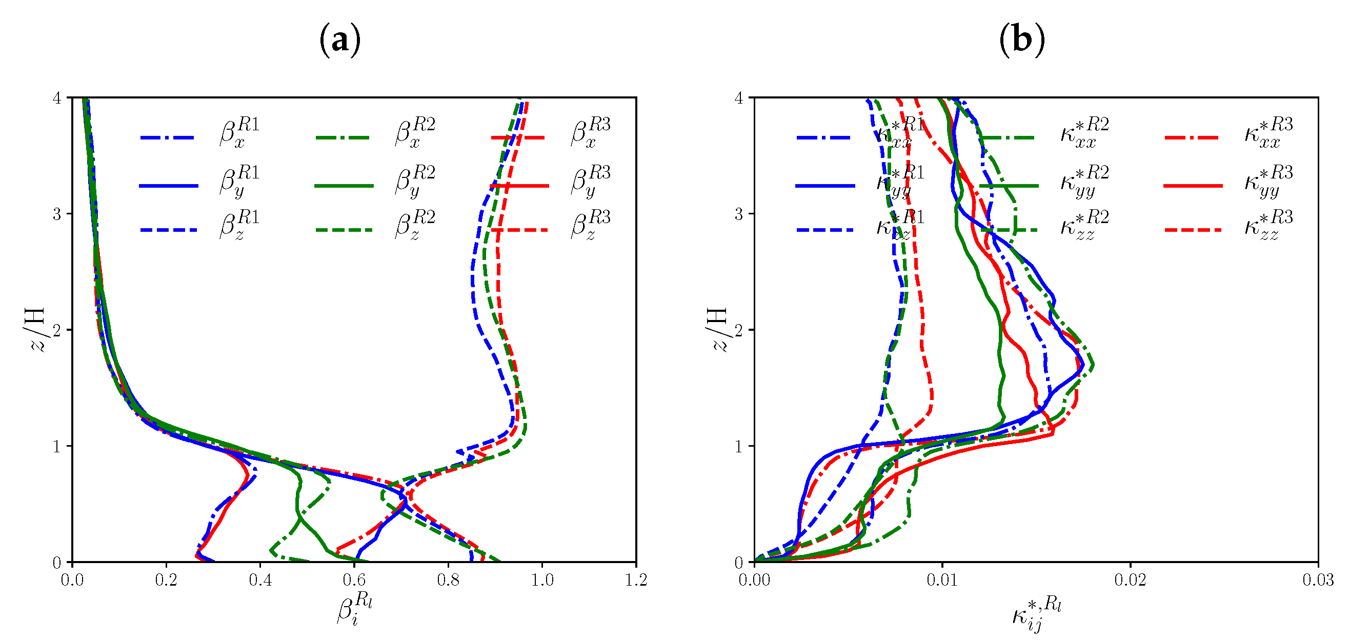
The effects of these two choices are now assessed. First, we consider vertical profiles of the turbulence coefficients, β i R l ( z ) (Figure A5a). 
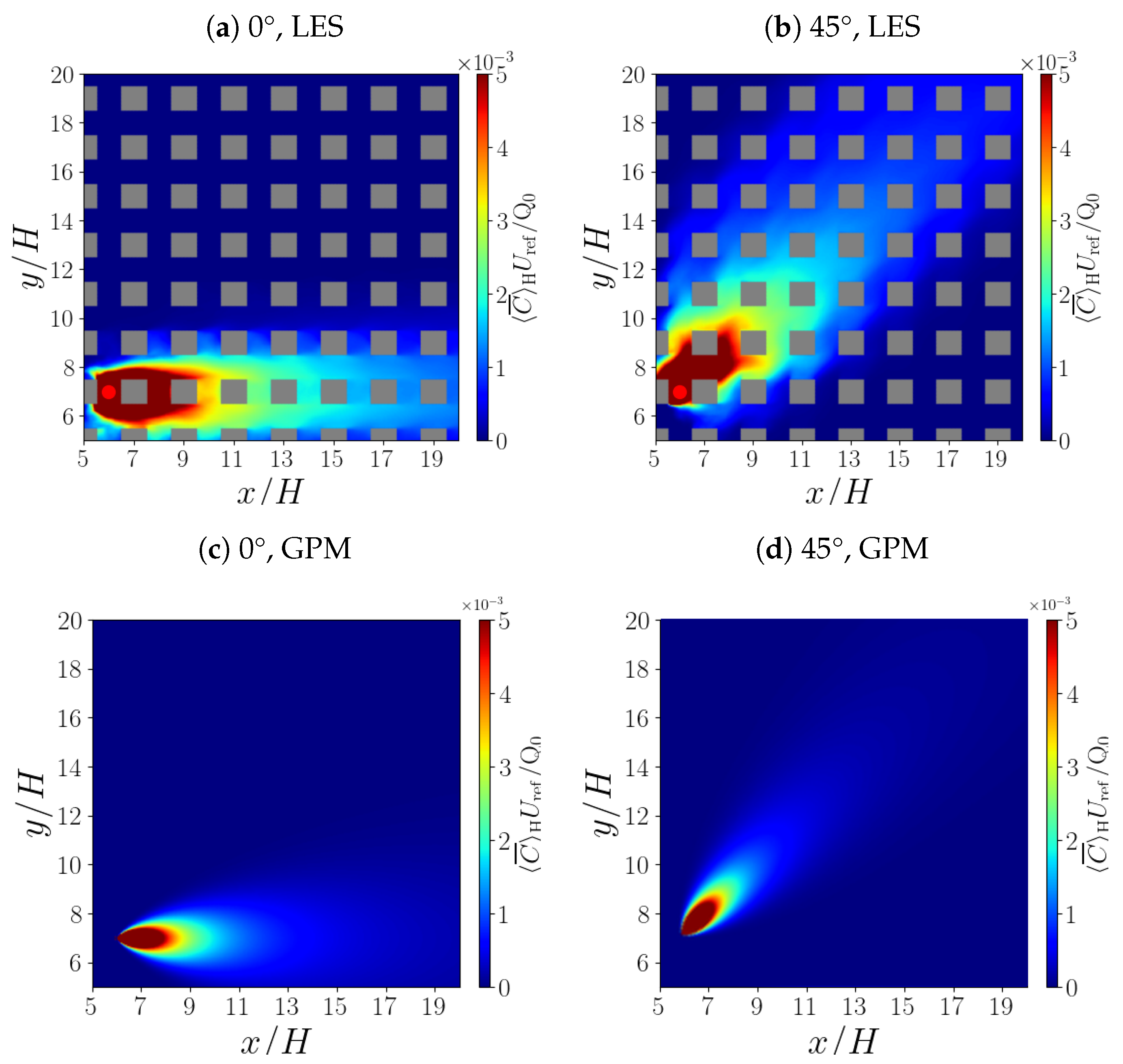
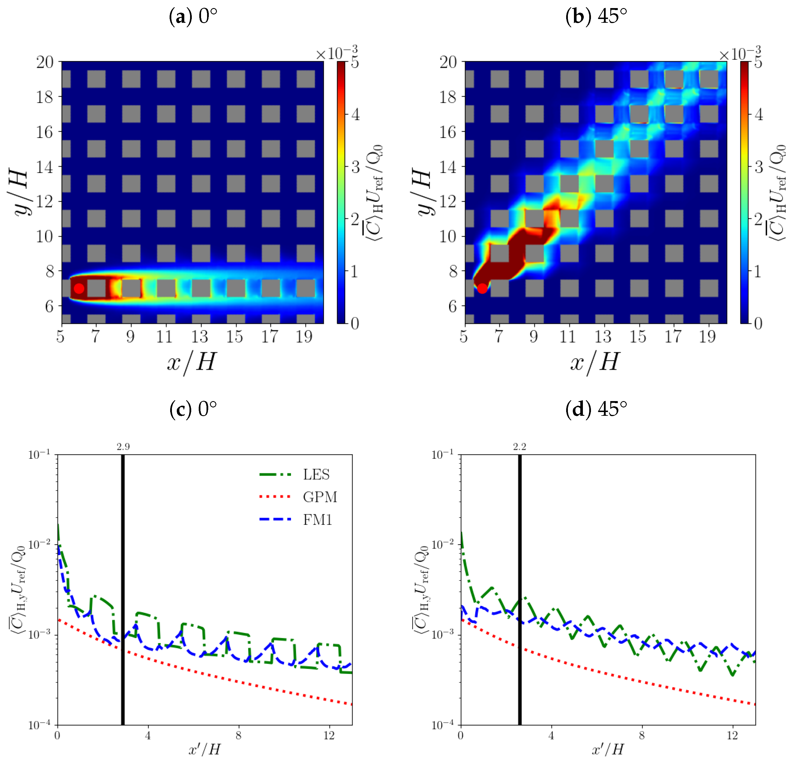
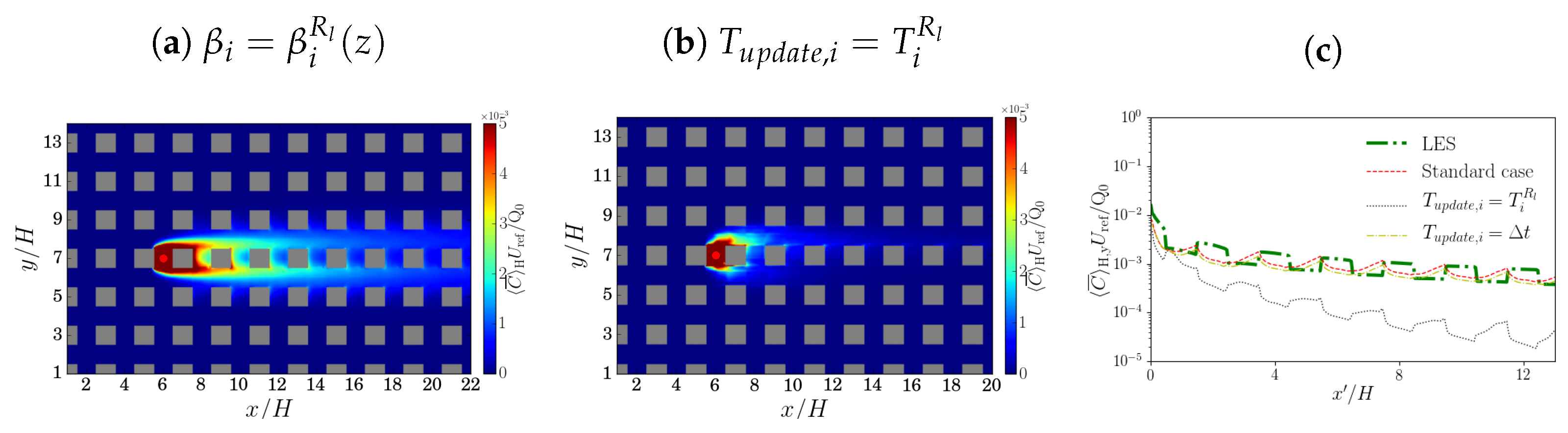
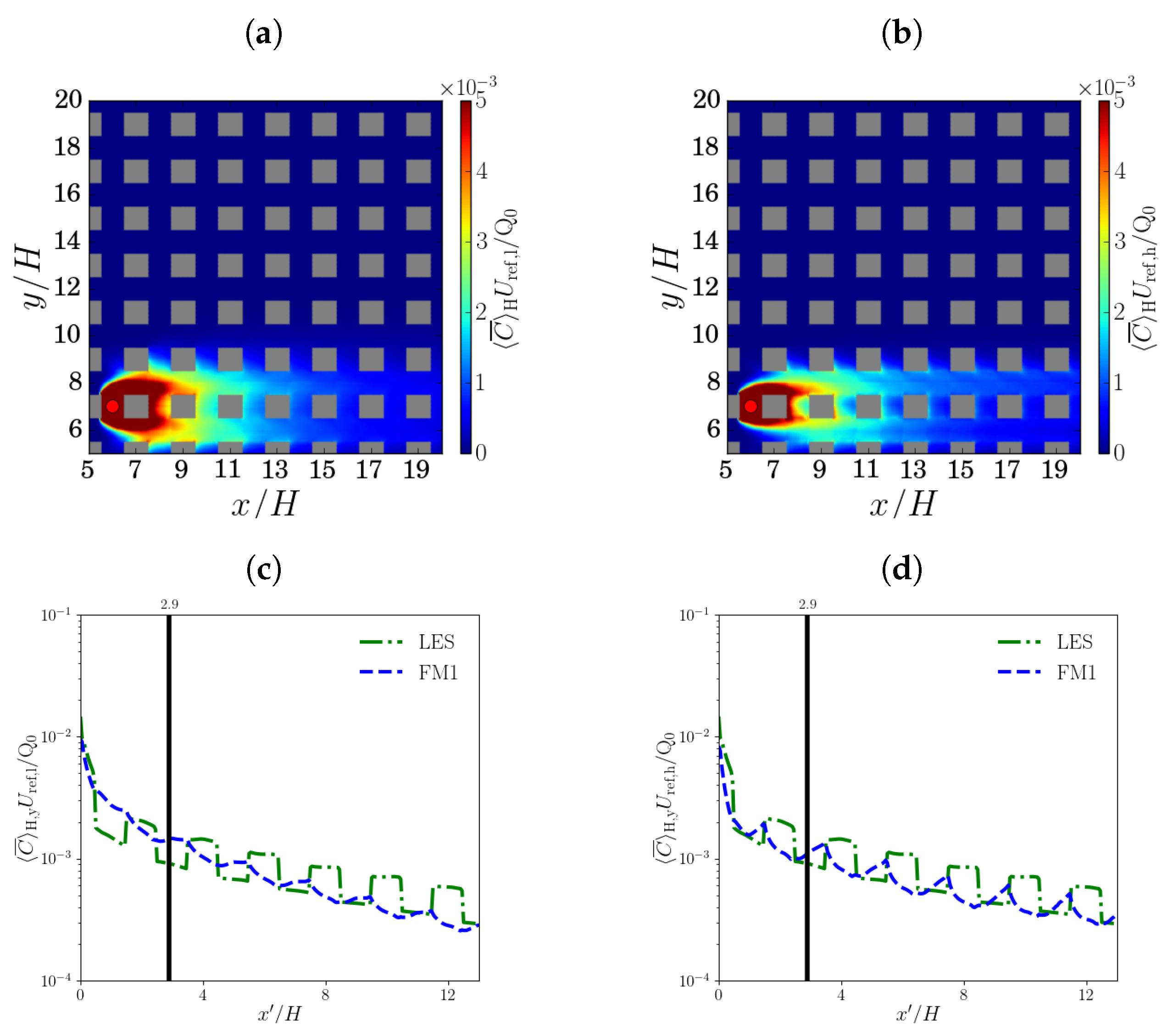
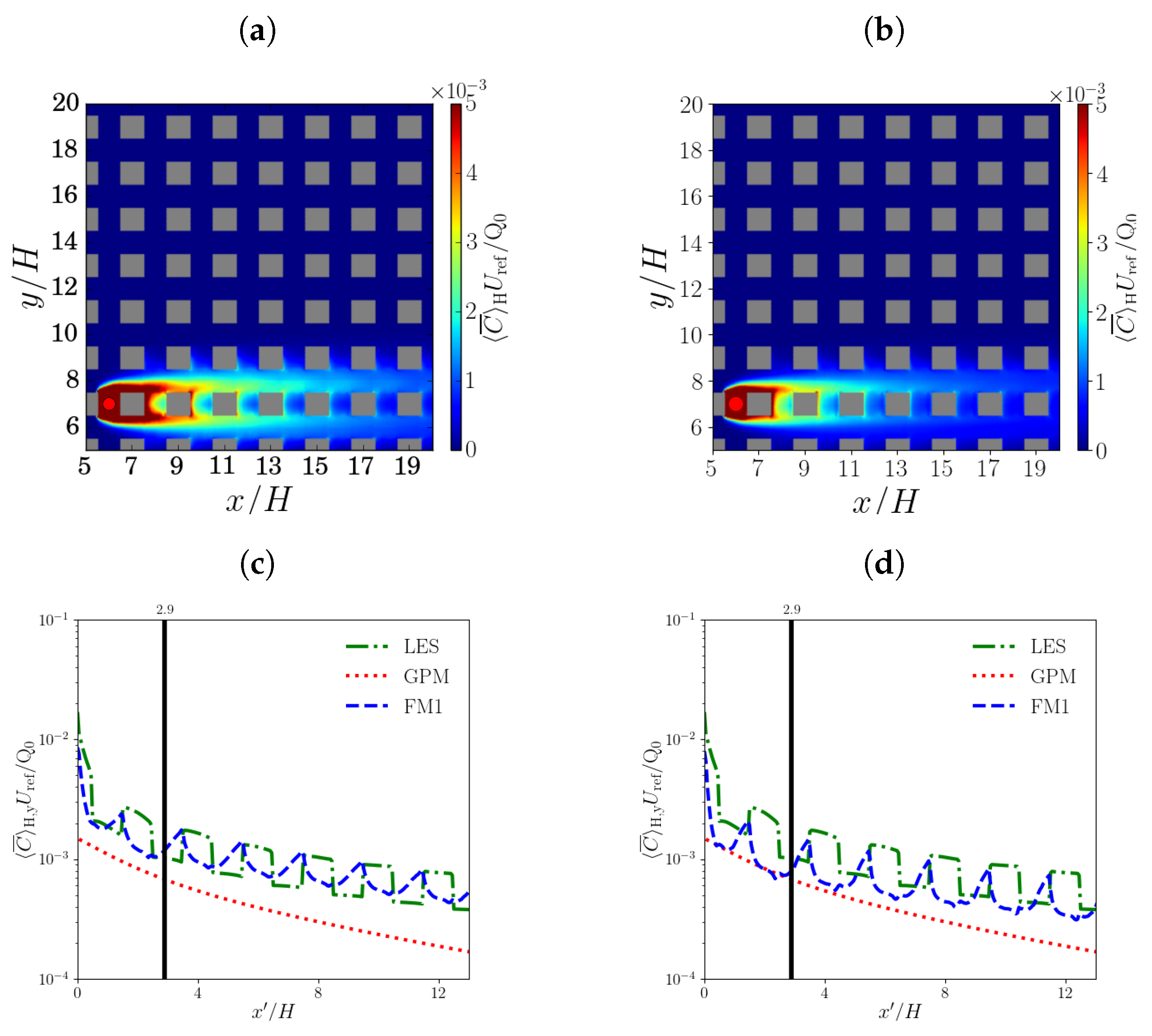
Figure 9a shows that the spatial structure of the mean concentration field at 0° is essentially unchanged from that for the standard configuration with β i , c a n o p y R l and β i , a b o v e (Figure 5a). Since the differences between β i R l ( z ) and β i , c a n o p y R l , β i , a b o v e are not very large (e.g., the maximum relative error is ∼50%), FM1 should not be especially sensitive to the inclusion of the vertical dependence of the turbulence coefficients. Indeed, the N M S E is 0.25 using β i , c a n o p y R l , β i , a b o v e (Table 1) and 0.51 with β i R l ( z ) (Table 2). It should be noted, however, that performance does not improve when the vertical dependence is specified. The reasons for this are unclear, but the change in the averaging region (from the canopy or overlying atmosphere to individual vertical levels) may play a role. The assumption that the turbulent fluctuations are linearly proportional to the mean velocity components (Equation (6)), which underlies the definition of the β , may break down on smaller vertical scales due to overfitting. Furthermore, the β ( z ) values are more subject to sampling effects.
Second, the turbulent fluctuations are updated at the e-folding timescale, i.e., T u p d a t e , i = T i R l . From the mean concentration field at 0° (Figure 9b), downwind dispersion is greatly reduced and the prediction is clearly worse. This is confirmed by the statistical metrics (Table 2): for example, N M S E increases from 0.25 (Table 1) to 1.96 when the turbulent fluctuations are updated at a time interval of T i R l rather than Δ t . Evidently choosing T u p d a t e , i to be as short as possible improves the prediction. This is plausible inasmuch as the SDE, Equation (8), is equivalent to a diffusion equation only in the limit of white noise, i.e., a vanishing correlation timescale [22]. Physically, defining the turbulence timescale from the e-folding timescale, like the related integral timescale [37], amounts to specifying a length scale; however, the SDE, or more generally Brownian motion, has no spatial dependence or spatial scales. The choice T u p d a t e , i = T i R l effectively imposes an artificially large length scale, which may be inconsistent with turbulent diffusion at the smallest possible scales.
The lateral profiles (Figure 9c) confirm the preceding findings. Prescribing the vertical profile of the turbulence coefficients, β i = β i R l ( z ) yields nearly identical results to the standard configuration, T u p d a t e , i = Δ t and β i = β i , c a n o p y R l , β i , a b o v e . Updating the turbulent fluctuations less frequently, i.e., T u p d a t e , i = T i R l , causes the profile to decay too rapidly with downwind distance. For brevity, the results for T u p d a t e , i = T i R l and β i = β i R l ( z ) are not shown because they are very similar to those for the preceding case, T u p d a t e , i = T i R l and β i = β i , c a n o p y R l , β i , a b o v e .
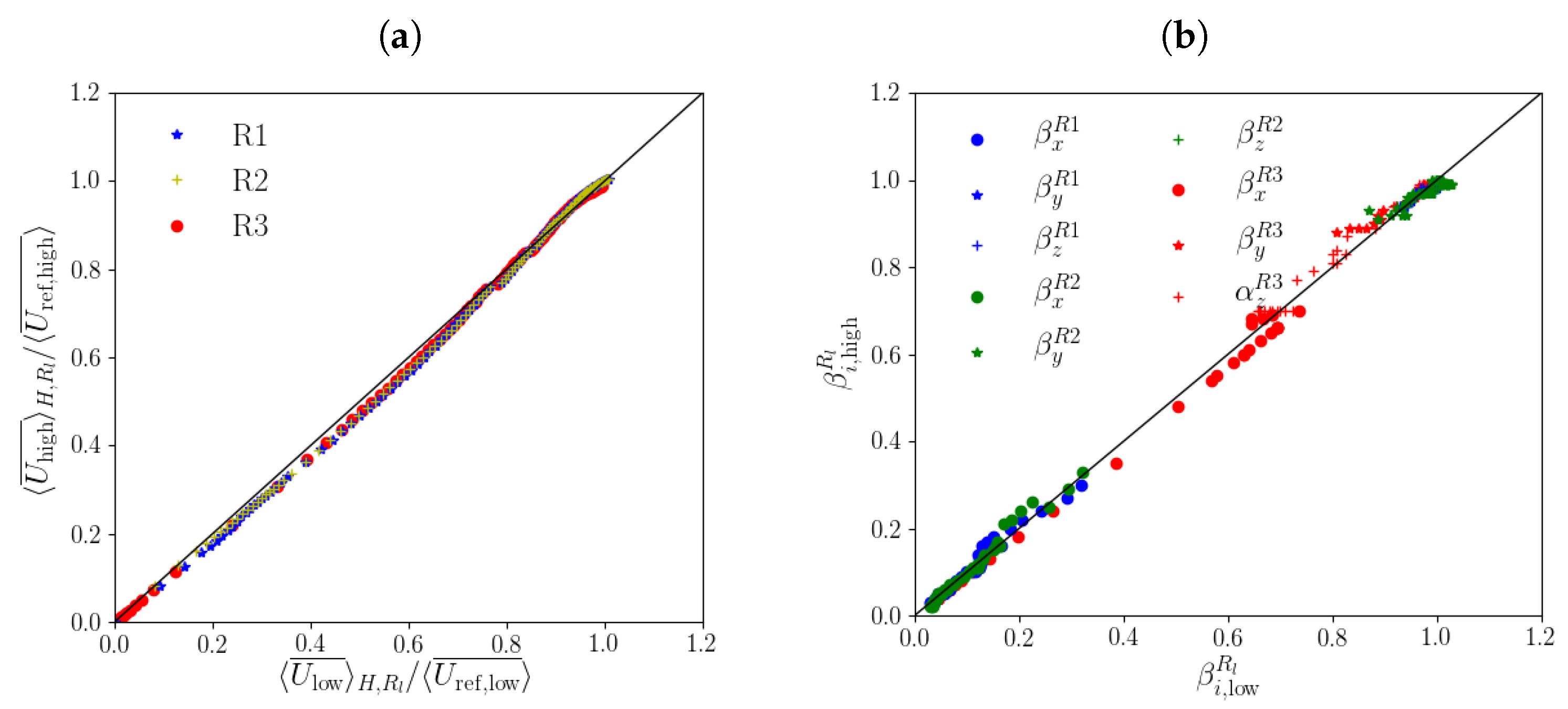
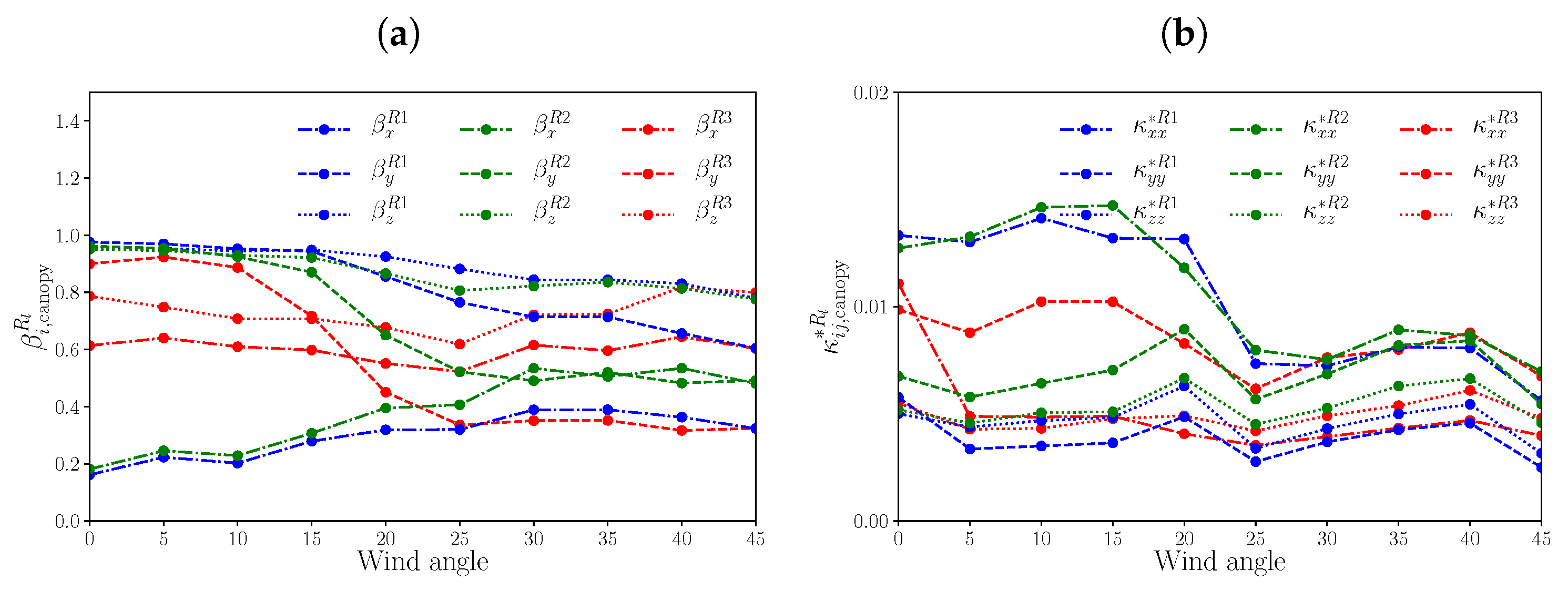
Aside from the vertical structure and correlation timescale, assumptions were also made about the horizontal structure and applicability to other wind directions. The dependence of β i , c a n o p y R l on the wind direction is illustrated in Figure 10a. Values are not independent of the angle. To assess the validity of the choice of 45° for the standard configuration, the turbulence coefficients for 0° (Table A9) are applied to an FM1 calculation for 0°. The scalar field (Figure A6a) shows enhanced cross-stream dispersion compared with the standard configuration; the lateral profile (Figure A6c) shows enhanced contrast between the windward and leeward walls. A slight degradation of the performance is seen in the statistical performance measures (Table 2), e.g., the NMSE increases from 0.25 to 0.37. Using the turbulence coefficients for the same wind direction does not necessarily help.
The sensitivity to the spatial variation of the β i , c a n o p y R l is assessed by considering the same turbulence coefficients for all repeating units β i , c a n o p y . Compared with β i , c a n o p y R l ( 0 ) , there are lower concentrations at the leeward walls (Figure A6b) and the concentration decays more rapidly in the downwind direction (Figure A6d). Neglecting the spatial variation of the turbulence coefficients has a negative impact: the N M S E increases from 0.25 to 0.74 (Table 2). Nevertheless, the sensitivity to the spatial variation of the turbulence coefficients is much smaller than that to a spatially varying mean flow.

6.2. FM2

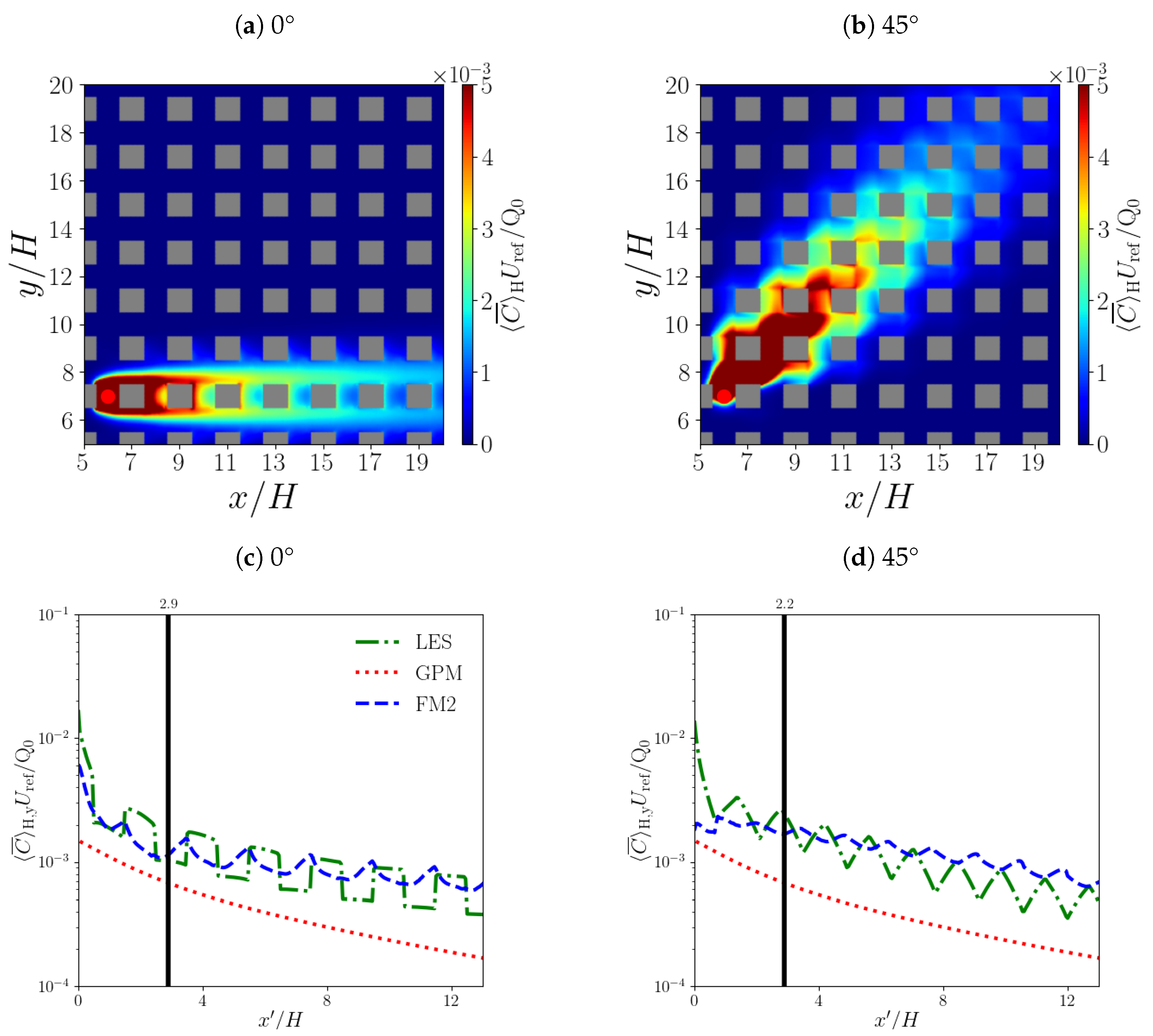
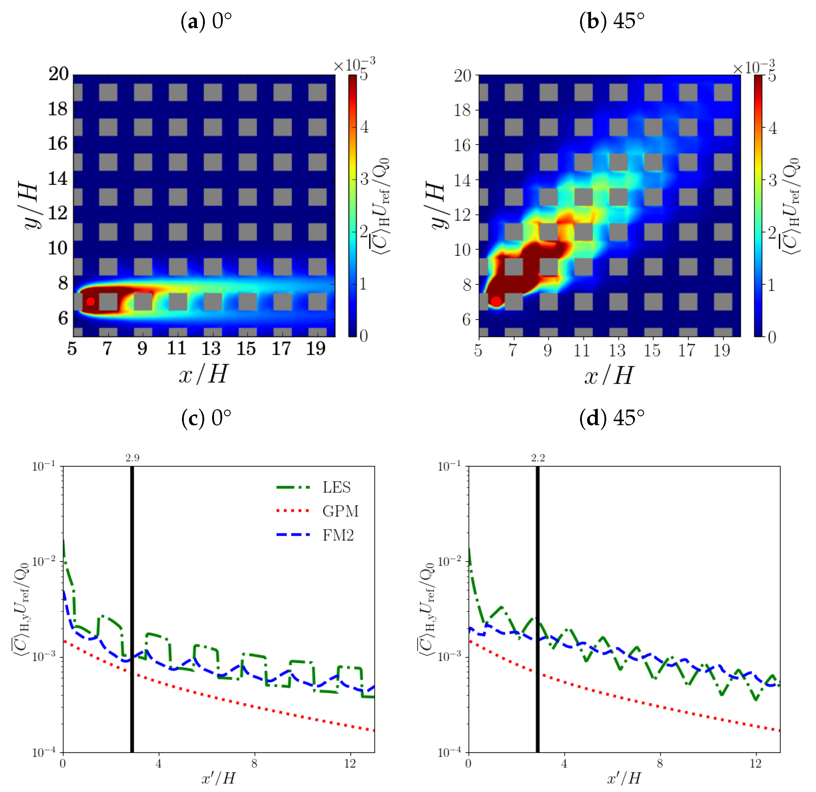
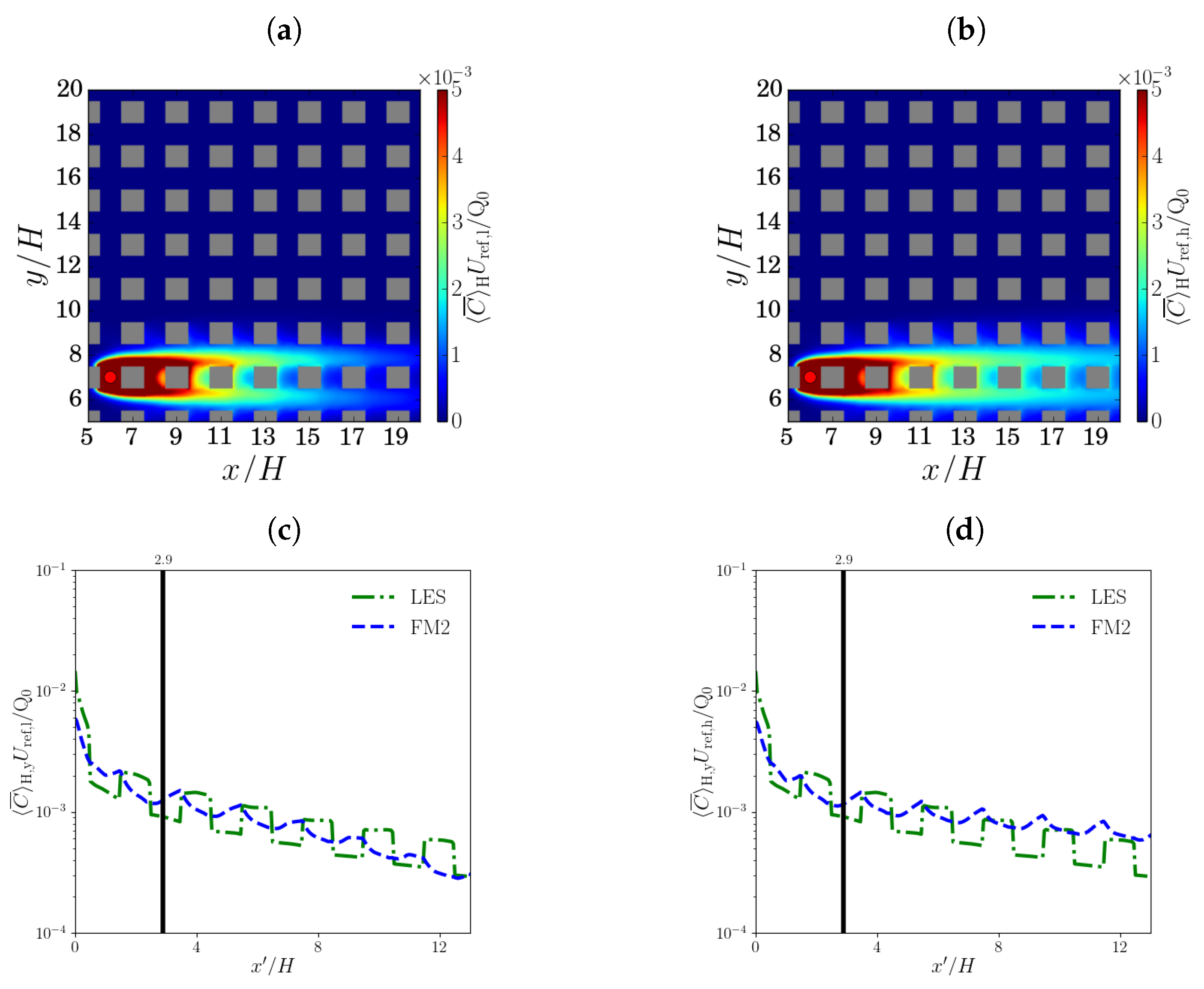
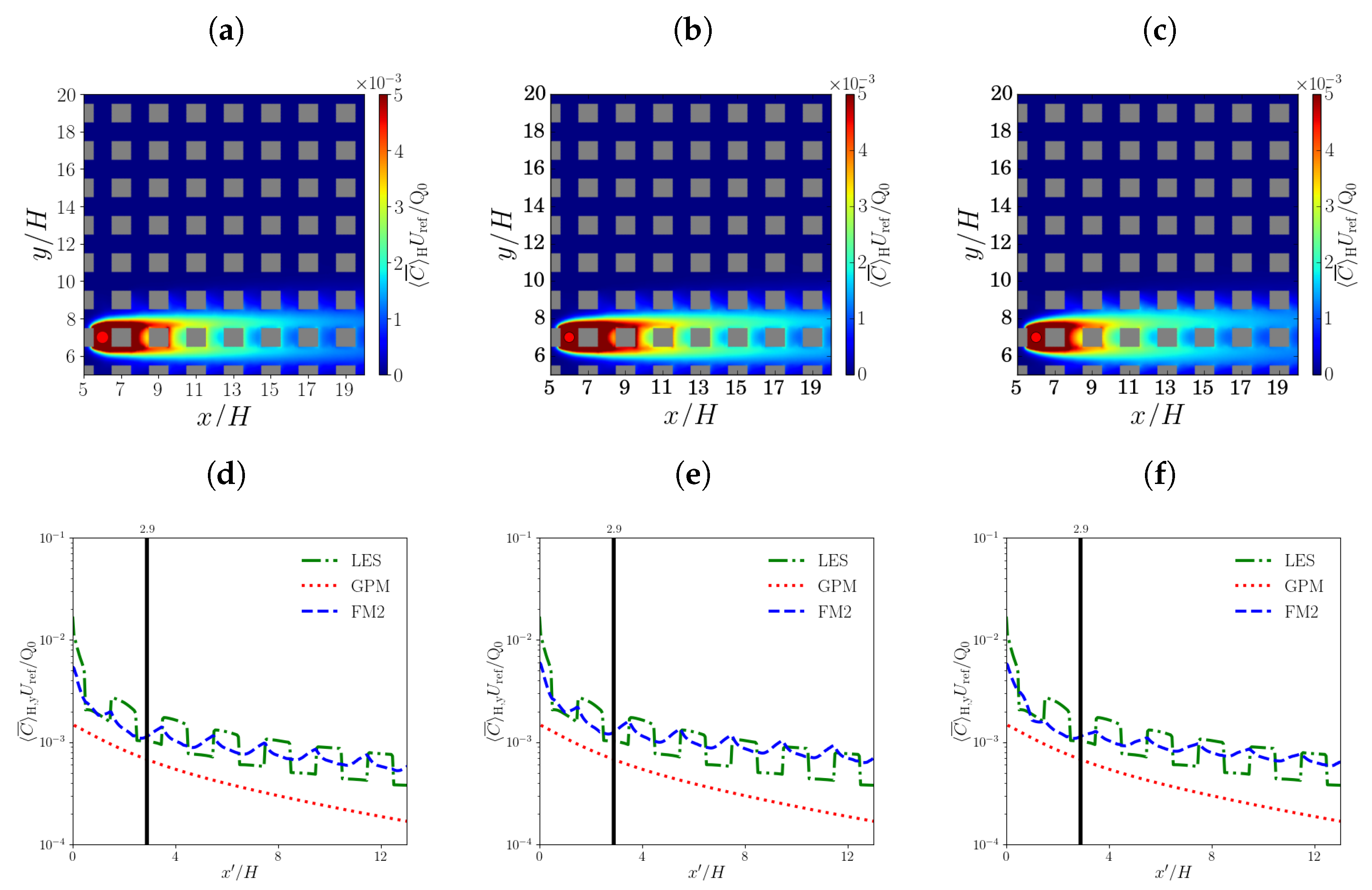
The default FM2 configuration also relies on spatial averages over the canopy and the overlying region to determine the effective diffusivities at 45°. Different specifications of the effective diffusivities are now applied to simulations for 0°.
First, prescribing the vertical profiles, κ i j R l ( z ) (Figure A5b), has a small effect on the scalar field (Figure A7a) and lateral profile (Figure A7d). The statistical metrics indicate a small degradation when the vertical profiles are used (e.g., NMSE increasing from 0.40 to 0.46; Table 2), as with FM1. Second, the effective diffusivities are defined using another wind direction. The assumption that κ i j , c a n o p y R l is independent of the angle is not accurate (Figure 10b). Hence, κ i j , c a n o p y R l ( 0 ) and κ i j , a b o v e ( 0 ) (Table A9) are tested in place of the effective diffusivities at 45°. The scalar field (Figure A7b) and lateral profile (Figure A7e) show higher downwind concentrations and the errors decrease slightly (Table 2). Third, horizontally averaged diffusivities, κ i j , c a n o p y , are used for all repeating units inside the canopy. Neglecting the spatial dependence lowers the concentrations along the leeward walls in the near-field region (Figure A7c) and weakens concentration gradients (Figure A7f). However, the statistical performance measures do not show much change (e.g., the N M S E decreases from 0.40 to 0.39).
The sensitivity to κ i j R l in FM2 is weaker than the sensitivity to β i R l in FM1. Not only does FM1 show great sensitivity to the correlation time, neglecting the dependence on the repeating units degrades performance. A possible explanation is that κ i j R l only affects diffusion, while β i R l affects advection and induces turbulent diffusion, which could lead to less robust behaviour.
The standard configuration of FM2 is limited to diagonal components of the effective diffusivity tensor, κ i j . Referring to the “microscopic” definition of the diffusivity, Equation (11), diagonal components, i = j , refer to motions arising from aligned fluctuations in the same direction. For a homogeneous medium and isotropic fluctuations, the off-diagonal components vanish, κ i j = 0 , i j = 0 , as with the molecular viscosity of a Newtonian fluid, but this is not necessarily true for an inhomogeneous medium or one with boundaries. Hence it is possible that a better parameterisation could be obtained if the effective diffusivity included off-diagonal contributions.
Off-diagonal components can be calculated in the same way as the diagonal components (i.e., using Equations (10) and (11) with T i j = Δ T ). Values for 0° and 45° are listed in 
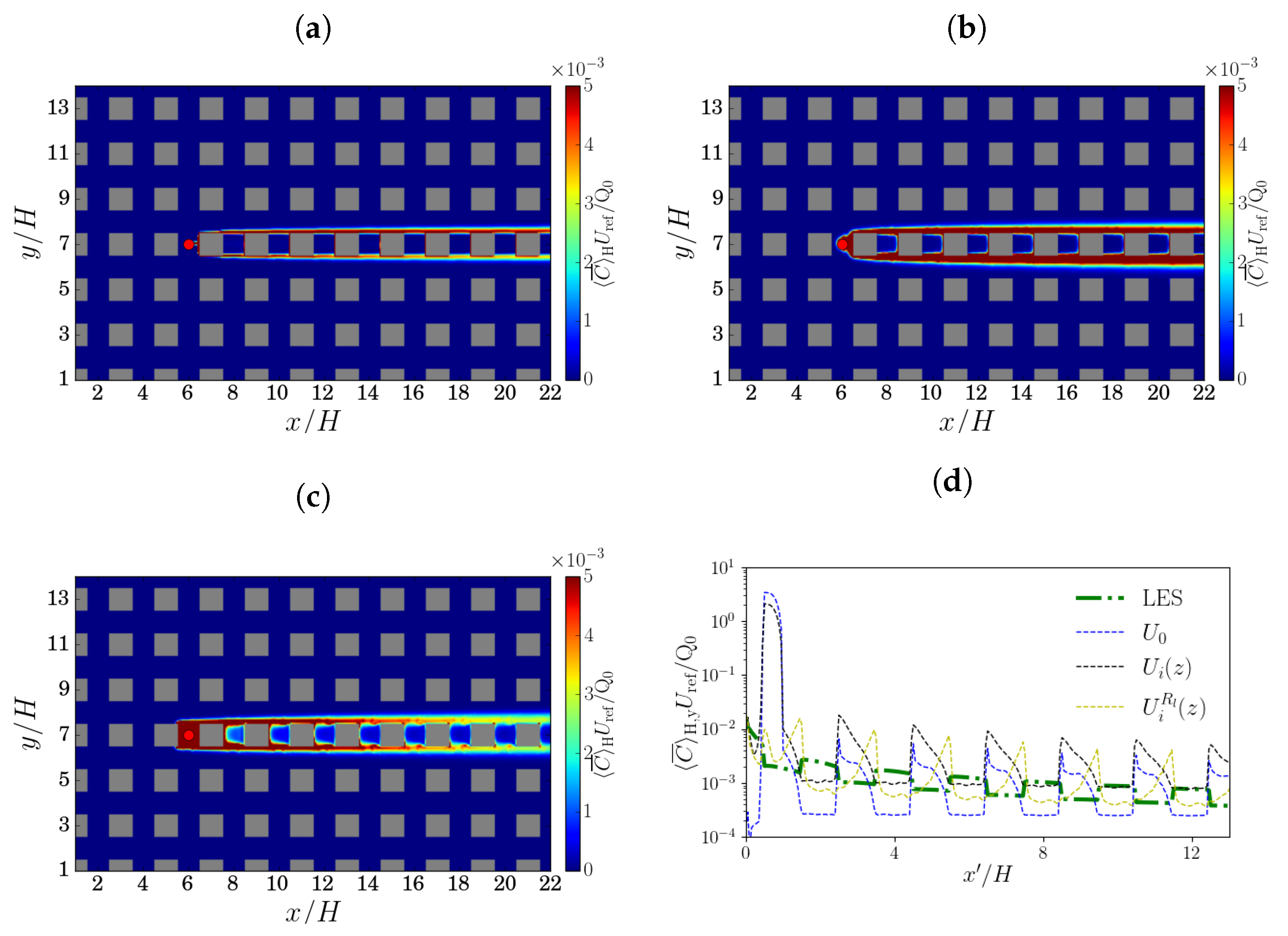
Table A10. The sensitivity to the inclusion of off-diagonal components is illustrated in Figure 11: at 0°, the scalar field is asymmetric along the centreline, while at 45°, there are minimal differences with respect to the standard configuration. The asymmetric appearance for 0° may be related to the K x y and K y x components, which are always positive for repeating units inside the canopy: these components introduce correlations between x and y fluctuations in the scalar field, i.e., anisotropy. The inclusion of the off-diagonal components clearly degrades performance at 0°; the effects are much smaller at 45°. This is confirmed by the statistical metrics (e.g., the NMSE inside the canopy increases from 0.40 to 0.74 in the former case and from 0.60 to 0.68 in the latter case; Table A5).
The negative impact of the off-diagonal components is perhaps surprising inasmuch as a parameterisation that takes fuller account of the turbulence statistics and does not require isotropy should perform better. A likely explanation is that the off-diagonal elements are assumed to be spatially uniform over a repeating unit. However, the non-zero off-diagonal components should be closely related to the local building geometry, which induces an inhomogeneous response. At 0°, u v differs in sign from one lateral boundary of a canyon unit to another (e.g., [38]); hence, K x y and K y x should be defined accordingly. Another contributing factor is sampling: at 45°, the values for the canyon and channel units are not identical, and the differences are comparable to or greater than those for the off-diagonal elements at 0°.

7. Discussion

The relatively good performance of the fast model can be attributed to the inclusion of spatially varying mean wind profiles. When it is assumed that the mean velocity is the same within all repeating units, the NMSE within the canopy is two to three orders of magnitude higher. Since air quality acceptance criteria (e.g., FAC2 0.5 , F B 0.3 , N M S E 0.3 ; [35]) are satisfied when the mean flow differs between repeating units, we conclude that the representation of the coarse-grained spatial variation of the mean flow is of primary importance. One may expect similar behaviour for domains that show comparable levels of spatial inhomogeneity. A simpler representation could be sufficient for an idealised street canyon; however, the importance of intersections to flow and dispersion within real cities is widely recognised [39].
The performance of the fast model is mostly insensitive to the choice of turbulence parameterisation. Temporally and spatially averaged fields from FM1 and FM2 show relatively small differences, as do the statistical metrics, when the correlation timescale is sufficiently short. Despite their different formulations, the models are largely equivalent: FM1 parameterises turbulent fluctuations directly; FM2 parameterises the turbulent diffusion arising from the turbulent fluctuations. Both approaches assume characteristic scales (e.g., the β i of FM1 and κ i j of FM2 are normalised) and neglect off-diagonal diffusivity or turbulent velocity fluctuations associated with a mean velocity component in another direction. The general insensitivity to their precise specification, as demonstrated by the sensitivity tests of Section 6, suggests that the assumptions underlying them are robust; however, the approaches are formally equivalent only in the limit of a vanishing timestep. FM1 and FM2 could deviate significantly for large timesteps, but the need to maintain a small Courant number helps ensure that the differences between them are small in practice. A small timestep mitigates differences associated with FM1 introducing fluctuations in the velocity field (which could introduce a drift over short time interval).
The fast model has two inherent limitations. First, it requires calibration to determine the geometric constants for the estimation of the mean velocity profiles and the coefficients for the turbulence parameterisations. This necessitates additional calculations, preferably from reference CFD simulations for a specific wind direction, which could limit the model’s applicability to other wind directions. The sensitivity tests for 0° and 45°, however, suggest that the turbulence coefficients and effective diffusivity for one wind direction can be applied to another. In any case, some form of calibration is almost unavoidable for simplified models that do not solve the governing equations: adjustable parameters are present in the GPM, as well as in fast dispersion models SIRANE [9] and QUIC [6]. Second, the spatial dependence of the mean velocity field inside each repeating unit is neglected while the turbulent fluctuations are spatially uncorrelated. The performance of the fast model suggests, however, that, at least for the cubic building array, fine-grained spatial structure is not essential. Averaging over repeating units should be an acceptable approximation so long as the spatial variability of the flow within them is not too great.
Although this study is limited to idealised configurations, its key components should be robust. The vortex method for the mean flow has already been extended to realistic building geometries [15]: the flow inside deep canopies is typically controlled by a few vortex sheets, which also facilitates calibration. The turbulence parameterisations have yet to be tested for more realistic domains, but they should perform comparably if the relationship between turbulent fluctuations and the mean flow does not differ significantly (cf. Equation (5)).
The fast model is unlikely to work well for a more realistic configuration if the nature of the turbulence should change from that for the cubic building array. One such scenario is unstable stratification (e.g., ground heating), for which convective plumes induce qualitative changes in the mean circulation and turbulence statistics [40]. Another is non-cuboidal buildings or ones with complex facade features for which the local turbulence will not be determined by the spatial average over a repeating unit. Nevertheless, the fast model should apply to realistic urban areas if the buildings are approximately cuboidal and the flow is neutral or stable.

8. Conclusions

The main finding of this study is that the dispersion of a passive scalar inside a cubic building array can be effectively modelled by combining estimated mean velocity profiles from a vortex method with a parameterization for turbulent diffusion based on introducing velocity fluctuations or specifying an effective diffusivity. Compared to reference LES simulations at 0° and 45°, the spatial structure of the steady (time-averaged) scalar field is largely captured while air quality acceptance criteria are satisfied. Although there is a relatively modest sacrifice in accuracy, computational efficiency is greatly increased. Table 3 compares the computational performance of both versions of the fast model with LES. FM1 and FM2 are ∼40–50 times faster than LES; the speed-up would be even greater if the LES spin-up were included in the comparison. FM2 is more computationally efficient because the numerical solution does not require the introduction of random fluctuations everywhere in the domain; moreover, sampling issues potentially arising from a finite timestep are avoided. Given its greater computational efficiency and simpler implementation, as well as the close agreement with FM1, FM2 is the better choice for most applications.
The most important implication is that urban pollutants can be modelled using a representation of the coarse-grained mean flow and turbulence. On one hand, this represents a significant simplification compared to direct CFD; on the other hand, the flow is represented far more accurately than in the Gaussian plume model or network models such as SIRANE [9] or MUNICH [10]. Any simplified or intermediate dispersion model necessarily involves simplification. In the fast model, dispersion inside the canopy is driven by the mean flow and turbulence varying on the scale of the building geometry. This is a multiscale modelling strategy which assumes that the flow is approximately constant over a finite region and that turbulent diffusion can be parameterised in terms of the mean velocity components: the use of the vortex method for the mean flow or the FM1 and FM2 turbulence parameterisations are not strictly required. Moreover, its applicability should extend beyond the cubic building array. While real urban canopies do not have repeating units, subdomains over which the mean flow and turbulence are approximately homogeneous could be defined empirically, though at the cost of added technical complexity. Nevertheless, the fast model should still work well for approximately grid-like neighbourhoods.
A secondary implication is that the fast model can be applied to time-critical applications such as operational air quality prediction or emergency dispersion modelling. Although calibration using reference CFD simulations is time-consuming, this could be performed in advance for problems in which the region of interest (e.g., a densely populated neighbourhood) is known, allowing for the FM’s computational efficiency to be realised in practice. If the building geometry were approximately uniform, as with the cubic building array, calibration could be limited to a small number of directions (or perhaps just a single one) as the turbulence coefficients and effective diffusivities should show minimal sensitivity to the wind direction.
There are several directions for future work. Most obviously, the method should be tested for more realistic geometries and flow configurations. As explained in the Discussion, there are good reasons for expecting the fast model’s applicability to extend beyond idealised flow over a cubic building array. Nevertheless, the extent of applicability needs to be determined. Furthermore, the turbulence parameterisations could be improved. A clear weakness of the fast model is that cross-stream dispersion is underpredicted for FM1 and FM2. This shortcoming could be partially ameliorated in the context of FM2 by allowing for correlations between turbulent fluctuations in different directions, which would amount to a proper specification of the off-diagonal components. For FM1 a more realistic stochastic parameterisation could be adopted [22]. Finally, more computationally efficient methods for solving the advection–diffusion equation could be explored. A Lagrangian stochastic method would be a natural choice for FM1.

Author Contributions

H.W.: Writing—Original draft preparation, Software, Validation, Visualization. E.F.-C.: Software, Validation, Reviewing. K.N.: Conceptualization, Supervision, Methodology, Formal analysis, Writing—Reviewing and Editing, Project administration, Funding acquisition. All authors have read and agreed to the published version of the manuscript.

Funding

This research was supported by the Research Grants Council of Hong Kong (CityU 11304517, CityU 11329616)) and the Environmental Protection Department of Hong Kong (Project 22-06813).

Institutional Review Board Statement

Not applicable.

Informed Consent Statement

Not applicable.

Data Availability Statement

Not applicable.

Conflicts of Interest

The authors declare that they have no known competing financial interest or personal relationships that could have appeared to influence the work reported in this paper.

Appendix A. Gaussian Plume Model (GPM)

The GPM yields a solution for the advection–diffusion equation given a pollutant emission rate (for a point source), atmospheric stability, wind speed and direction. The main assumptions are as follows:
  • The velocity is a constant, u = ( u , 0 , 0 ) .
  • The eddy diffusivities, K i ( x ) , are isotropic and functions of the downwind distance x only.
  • Diffusion is weak compared to advection in the streamwise (x) direction.
  • The pollutant does not penetrate the ground.
  • There are Dirichlet boundary conditions at the lateral edges, C ( 0 , y , z ) = 0 , C ( , y , z ) = 0 , C ( x , ± , z ) = 0 , C ( x , y , ) = 0 .
  • There is a Neumann boundary condition C z ( x , y , 0 ) = 0 at the ground.
  • The source is located at a height H 0 .
The steady solution for the concentration may be written as
C ( x , y , z ) = Q 2 π u σ y σ z exp ( y 2 2 σ y 2 ) exp ( ( z H ) 2 2 σ z 2 ) + exp ( ( z + H ) 2 2 σ z 2 ) .
The standard deviations, σ y 2 and σ z 2 , depend on the atmospheric stability. Assuming neutral stability, σ y = a x b , σ z = c x d + f , where a = 156 , b = 0.89 , c = 108.2 , d = 1.098 and f = 2.0 [41].

Appendix B. Validation of the LES Model

Appendix B.1. Velocity Statistics

The mean streamwise velocity predicted by the LES model described in Section 3.2 is validated against wind-tunnel measurements of flow over a regular array of cubic buildings [42]. Vertical profiles of the mean streamwise velocity measured at the center of canyon units are compared in Figure A1. There is good agreement above the ground, i.e., z / H > 0.1 .
Statistical performance measures (Appendix C) confirm that the LES model simulates the mean wind profile accurately (Table Figure A1). The NMSE and F B are close to 0 and the correlation coefficient is close to 1.
Table A1. Statistical performance measures corresponding to Figure A1. the temporally averaged streamwise velocity. The mean streamwise velocity and rms streamwise velocity fluctuation at the centre of a canyon unit are compared to the wind-tunnel data of [42].
FB MG NMSE VG R FAC 2
Streamwise velocityu−0.0600.9510.0501.0110.9700.960
Figure A1. Validation of mean streamwise velocity predicted by LES (dotted line) against wind-tunnel data of Uehara et al. (2000) (blue stars) [42].
Atmosphere 14 01337 g0a1

Appendix B.2. Concentration Statistics

Concentration statistics generated by a point source located at the centre of a unit-aspect-ratio street canyon are validated using experimental data [43]. The lateral profiles show good agreement (Figure A2). This is confirmed by the statistical metrics (Table A2). Hence, we conclude that the LES model is also capable of simulating the dispersion from a point source.
Figure A2. Lateral concentration profiles generated by a point source within a street canyon: LES (dashed-dotted line) is compared to the wind-tunnel data of Hildemann and Chong 2007 (blue dots) [43]. (a) ( x x s ) = 2 H , z = 0.25 H . (b) ( x x s ) = 6 H , z = 0.25 H .
Atmosphere 14 01337 g0a2
Table A2. Statistical performance measures corresponding to Figure A2. The scalar statistics comprise spanwise profiles at x 1 = x s + 2 H and x 2 = x s + 6 H , where x s is the source location.
FB MG NMSE VG R FAC 2
Passive scalar c ( x 1 , z = 0.25 H ) 0.0670.9440.0201.1280.9870.902
c ( x 2 , z = 0.25 H ) −0.0390.8480.0141.0940.9900.972

Appendix C. Statistical Performance Measures

Appendix C.1. Definitions

In order to validate the simulation data ( D s ) against measurements ( D e ), we calculate the following statistical performance measures [35]: fractional bias ( F B ),
F B = ( D e ¯ D s ¯ ) 0.5 ( D e ¯ + D s ¯ ) ,
geometric mean bias ( M G ),
M G = exp ( ln D e ¯ ln D s ¯ ) ,
normalized mean square error ( N M S E ),
N M S E = ( D e D s ) 2 ¯ D e D s ¯ ,
geometric variance (VG),
V G = exp [ ( ln D e ln D s ) 2 ¯ ] ,
correlation coefficient (R),
R = ( D e D e ¯ ) ( D s D s ¯ ) ¯ σ D e σ D s ,
and fraction of data within a factor of two ( F A C 2 ),
F A C 2 = 1 N i = 0 N 1 χ i , where χ i = 1 , for 0.5 D e / D s 2.0 , 0 , otherwise .
The overbar represents average over the dataset and σ D e , σ D s are the standard deviations. For a perfect validation, F B = N M S E = 0.0 and M G = V G = R = F A C 2 = 1.0 .

Appendix C.2. Application to Lateral Profiles

Table A3. Statistical evaluation of FM performance at 0° inside the canopy (with respect to the LES baseline) for low and high reference wind speeds.
FB MG NMSE VG R FAC 2
FM1, U ref , low = 1 ms 1 Near field−0.060.830.211.210.910.91
Far field0.171.240.211.210.680.86
Entire field0.051.140.341.210.910.87
FM1, U ref , high = 9 ms 1 Near field0.331.250.301.20.930.90
Far field0.211.220.211.200.600.93
Entire field0.271.220.291.200.920.92
FM2, U ref , low = 1 ms 1 Near field0.221.050.381.180.910.98
Far field0.061.100.141.180.700.93
Entire field0.141.090.331.180.880.94
FM2, U ref , high = 9 ms 1 Near field0.271.100.421.170.910.98
Far field−0.210.740.141.240.660.84
Entire field−0.010.800.351.220.910.86
Table A4. As in Table A3, but the FM performance of different mean flow prescriptions is evaluated.
FB MG NMSE VG R FAC 2
Constant streamwise wind speed−1.951.151374.5442.120.090.15
Uniform velocity profile−1.910.38782.8424.890.100.45
Different velocity profile within each repeating unit−0.320.941.312.510.480.45
Table A5. As in Table A3, but for FM2 with an effective diffusivity tensor containing off-diagonal components.
FB MG NMSE VG R FAC 2
FM2Near field0.621.640.911.450.930.55
Far field0.211.160.191.160.591.0
Entire field0.391.240.741.210.920.91
45°Near field0.551.561.061.450.190.84
Far field−0.020.930.091.090.821.0
Entire field0.211.030.681.150.680.96

Appendix D. Additional Tables and Figures

Table A6. Dimensionless turbulence coefficients for FM1.
β i , canopy R l , z / H [ 0 , 1 ] β i , above , z / H [ 1 , 5 ]
θ i Channel UnitIntersection UnitCanyon UnitAbove Canopy
x0.140.150.580.01
y0.980.960.890.98
z0.950.950.770.98
45°x0.330.480.560.05
y0.560.480.330.05
z0.780.750.780.93
Table A7. Normalised effective diffusivities for FM2.
κ ij , canopy R l , z / H [ 0 , 1 ] κ ij , above , z / H [ 1 , 5 ]
θ ij Channel UnitIntersection UnitCanyon UnitAbove Canopy
x x 0.01450.01530.00530.0168
y y 0.00330.00580.01050.0102
z z 0.00430.00480.00500.0082
45° x x 0.00410.00470.00330.0167
y y 0.00290.00550.00400.0127
z z 0.00320.00450.00360.0075
Table A8. Turbulence correlation timescales, T i R l , determined from LES data for 0° and 45°.
T i , canopy R l , z / H [ 0 , 1 ] T i , above , z / H [ 1 , 5 ]
θ i Channel UnitIntersection UnitCanyon UnitAbove Canopy
(s)(s)(s)(s)
T x 5.75.26.05.0
T y 5.05.27.05.0
T z 5.05.16.35.4
45° T x 5.85.36.35.1
T y 4.95.36.95.0
T z 5.05.16.35.4
Table A9. Turbulence coefficients, β i , c a n o p y R l , and normalised effective diffusivities, κ i j R l for 0° and 45°.
β i , canopy R l , z / H [ 0 , 1 ] β i , above , z / H [ 1 , 5 ]
θ i Channel UnitIntersection UnitCanyon UnitAbove Canopy
β x 0.140.150.580.01
β y 0.980.960.890.98
β z 0.950.950.770.98
45° β x 0.330.480.560.05
β y 0.560.480.330.05
β z 0.780.750.780.93
κ x x 0.01450.01530.00530.0168
κ y y 0.00330.00580.01050.0102
κ z z 0.00430.00480.00500.0082
45° κ x x 0.00410.00470.00330.0167
κ y y 0.00290.00550.00400.0127
κ z z 0.00320.00450.00360.0075
Table A10. Normalised effective diffusivity tensors, κ i j , c a n o p y and κ i j , a b o v e . Note that all nine components are included for each entry.
κ ij , canopy R l , z / H [ 0 , 1 ]
R l Channel UnitIntersection UnitCanyon Unit
   0° 0.0145 0.0008 0.0001 0.0008 0.0033 0.0008 0.0001 0.0008 0.0043 0.0153 0.0003 0.0004 0.0003 0.0058 0.0013 0.0013 0.0004 0.0048 0.0053 0.0003 0.0014 0.0003 0.0105 0.0011 0.0014 0.0011 0.0050
   45° 0.0041 0.0008 0.0002 0.0008 0.0029 0.0008 0.0002 0.0008 0.0032 0.0047 0.0017 0.0003 0.0017 0.0055 0.0017 0.0003 0.0017 0.0045 0.0033 0.0005 0.0001 0.0005 0.0040 0.001 0.0001 0.001 0.0036
κ i j , a b o v e , z / H [ 1 , 5 ]   
Above canopy  
   0° 0.0168 0.0024 0.0018 0.0024 0.0102 0.0010 0.0018 0.0010 0.0082   
   45° 0.0167 0.0016 0.0025 0.0016 0.0127 0.0017 0.0025 0.0017 0.0075   
Figure A3. Mean concentration fields (top) and lateral profiles (bottom) at low and high reference wind speeds for FM1 and 0°: (a,c) U ref , low = 1 ms 1 ; (b,d) U ref , high = 9 ms 1 . In all cases, the baseline turbulence coefficients for U ref = 3 ms 1 were used.
Atmosphere 14 01337 g0a3
Figure A4. As in Figure A3, but for FM2. (a,c) U ref , low = 1 ms 1 ; (b,d) U ref , high = 9 ms 1 . κ i j R l for U ref = 3 ms 1 is used for U ref = 1 ms 1 and U ref = 9 ms 1 .
Atmosphere 14 01337 g0a4
Figure A5. Vertical profiles of fast model parameters at 45°: (a) turbulence coefficients, β i R l ; (b) normalised effective diffusivities, κ i j R l . R l labels the repeating units, i.e., channel (R1), intersection (R2) and canyon (R3).
Atmosphere 14 01337 g0a5
Figure A6. Mean concentration fields and lateral profiles for FM1 at 0° using modified configurations: (a,c) Turbulence coefficients obtained at 0° (rather than 45°), β i R l ( 0 ) ; (b,d) turbulence coefficients are the same for all repeating units, β i , c a n o p y .
Atmosphere 14 01337 g0a6
Figure A7. Mean concentration fields and lateral profiles for FM2 at 0° using modified configurations: (a,d) effective diffusivity is a function of height, κ i j R l ( z ) ; (b,e) effective diffusivity is calculated at 0°, i.e., κ i j , c a n o p y R l ( 0 ) and κ i j , a b o v e ( 0 ) ; (c,f) effective diffusivity is horizontally averaged over the repeating units, κ i j , c a n o p y .
Atmosphere 14 01337 g0a7

References

  1. Wang, H.; Ngan, K. Effects of inhomogeneous ground-level pollutant sources under different wind directions. Environ. Pollut. 2021, 289, 117903. [Google Scholar] [CrossRef] [PubMed]
  2. Baik, J.J.; Park, S.B.; Kim, J.J. Urban flow and dispersion simulation using a CFD model coupled to a mesoscale model. J. Appl. Meteorol. Climatol. 2009, 48, 1667–1681. [Google Scholar] [CrossRef]
  3. Kurppa, M.; Hellsten, A.; Auvinen, M.; Raasch, S.; Vesala, T.; Järvi, L. Ventilation and air quality in city blocks using large-eddy simulation-urban planning perspective. Atmosphere 2018, 9, 65. [Google Scholar] [CrossRef]
  4. Sutton, O.G. A theory of eddy diffusion in the atmosphere. Proc. R. Soc. Lond. 1932, 135, 143–165. [Google Scholar]
  5. Stockie, J.M. The mathematics of atmospheric dispersion modeling. SIAM Rev. 2011, 53, 349–372. [Google Scholar] [CrossRef]
  6. Singh, B.; Hansen, B.S.; Brown, M.J.; Pardyjak, E.R. Evaluation of the QUIC-URB fast response urban wind model for a cubical building array and wide building street canyon. Environ. Fluid Mech. 2008, 8, 281–312. [Google Scholar] [CrossRef]
  7. Williams, M.D.; Brown, M.; Boswell, D.; Singh, B.; Pardyjak, E. Testing of the QUIC-PLUME model with wind-tunnel measurements for a high-rise building. In Proceedings of the Fifth AMS Symposium on the Urban Environment, Vancouver, BC, Canada, 23–26 August 2004; American Meteorological Society: Boston, MA, USA, 2004. [Google Scholar]
  8. Kochanski, A.K.; Pardyjak, E.R.; Stoll, R.; Gowardhan, A.; Brown, M.J.; Steenburgh, W.J. One-Way Coupling of the WRF—QUIC Urban Dispersion Modeling System. J. Appl. Meteorol. Climatol. 2015, 54, 2119–2139. [Google Scholar] [CrossRef]
  9. Soulhac, L.; Salizzoni, P.; Cierco, F.X.; Perkins, R. The model SIRANE for atmospheric urban pollutant dispersion; Part I, presentation of the model. Atmos. Environ. 2011, 45, 7379–7395. [Google Scholar] [CrossRef]
  10. Kim, Y.; Wu, Y.; Seigneur, C.; Roustan, Y. Multi-scale modeling of urban air pollution: Development and application of a Street-in-Grid model (v1.0) by coupling MUNICH (v1.0) and Polair3D (v1.8.1). Geosci. Model Dev. 2018, 11, 611–629. [Google Scholar] [CrossRef]
  11. Soulhac, L.; Salizzoni, P.; Mejean, P.; Didier, D.; Rios, I. The model SIRANE for atmospheric urban pollutant dispersion; Part II, validation of the model on a real case study. Atmos. Environ. 2012, 49, 320–337. [Google Scholar] [CrossRef]
  12. Lugon, L.; Sartelet, K.; Kim, Y.; Vigneron, J.; Chrétien, O. Nonstationary modeling of NO2, NO and NOx in Paris using the Street-in-Grid model: Coupling local and regional scales with a two-way dynamic approach. Atmos. Chem. Phys. 2020, 20, 7717–7740. [Google Scholar] [CrossRef]
  13. Furtak-Cole, E.; Ngan, K. Predicting mean velocity profiles inside urban canyons. J. Wind Eng. Ind. Aerodyn. 2020, 207, 104280. [Google Scholar] [CrossRef]
  14. Pavliotis, G.; Stuart, A. Multiscale Methods: Averaging and Homogenization; Springer: Berlin/Heidelberg, Germany, 2008. [Google Scholar]
  15. Wang, H.; Furtak-Cole, E.; Ngan, K. Estimating mean wind profiles inside realistic urban Canopies. Atmosphere 2023, 14, 50. [Google Scholar] [CrossRef]
  16. Saffman, P.G. Vortex Dynamics; Cambridge University Press: Cambridge, UK, 1992. [Google Scholar]
  17. Wu, J.Z.; Ma, H.Y.; Zhou, M.D. Vorticity and Vortex Dynamics; Springer Science & Business Media: Berlin/Heidelberg, Germany, 2007. [Google Scholar]
  18. Flierl, G.R. Isolated eddy models in geophysics. Annu. Rev. Fluid Mech. 1987, 19, 493–550. [Google Scholar] [CrossRef]
  19. Pullin, D.I. Contour Dynamics Methods. Annu. Rev. Fluid Mech. 1992, 24, 89–115. [Google Scholar] [CrossRef]
  20. Raupach, M.R.; Shaw, R.H. Averaging procedures for flow within vegetation canopies. Bound.—Layer Meteorol. 1982, 22, 79–90. [Google Scholar] [CrossRef]
  21. Coceal, O.; Thomas, T.; Castro, I.; Belcher, S. Mean flow and turbulence statistics over groups of urban-like cubical obstacles. Bound.—Layer Meteorol. 2006, 121, 491–519. [Google Scholar] [CrossRef]
  22. Rodean, H.C. Stochastic Lagrangian Models of Turbulent Diffusion; American Meteorological Society: Boston, MA, USA, 1996. [Google Scholar]
  23. Majda, A.J.; Kramer, P.R. Simplified models for turbulent diffusion: Theory, numerical modelling, and physical phenomena. Phys. Rep. 1999, 314, 237–574. [Google Scholar] [CrossRef]
  24. Leelossy, Á.; Molnár, F.; Izsák, F.; Havasi, Á.; Lagzi, I.; Mészáros, R. Dispersion modeling of air pollutants in the atmosphere: A review. Open Geosci. 2014, 6, 257–278. [Google Scholar] [CrossRef]
  25. Blocken, B. Computational Fluid Dynamics for urban physics: Importance, scales, possibilities, limitations and ten tips and tricks towards accurate and reliable simulations. Build. Environ. 2015, 91, 219–245. [Google Scholar] [CrossRef]
  26. Robins, A.; MacDonald, R. Review of Flow and Dispersion in the Vicinity of Groups of Buildings, Annexe B, Atmospheric Dispersion Modelling Liaison Committee; Annual Report 1998/99, NRPB R-322. 2001. Available online: https://admlc.files.wordpress.com/2014/05/2001_nrpbr322_all.pdf (accessed on 25 July 2023).
  27. Goulart, E.V.; Coceal, O.; Branford, S.; Thomas, T.; Belcher, S. Spatial and temporal variability of the concentration field from localized releases in a regular building array. Bound.—Layer Meteorol. 2016, 159, 241–257. [Google Scholar] [CrossRef]
  28. Wang, H.; Brimblecombe, P.; Ngan, K. A numerical study of local traffic volume and air quality within urban street canyons. Sci. Total Environ. 2021, 791, 148138. [Google Scholar] [CrossRef] [PubMed]
  29. Moukalled, F.; Mangani, L.; Darwish, M. The Finite Volume Method in Computational Fluid Dynamics; Springer: Berlin/Heidelberg, Germany, 2016. [Google Scholar]
  30. Nicoud, F.; Ducros, F. Subgrid-scale stress modelling based on the square of the velocity gradient tensor. Flow Turbul. Combust. 1999, 62, 183–200. [Google Scholar] [CrossRef]
  31. Spalding, D.B. A single formula for the law of the wall. J. Appl. Mech. 1961, 28, 455–458. [Google Scholar] [CrossRef]
  32. Zhang, Y.; Yang, X.; Yang, H.; Zhang, K.; Wang, X.; Luo, Z.; Hang, J.; Zhou, S. Numerical investigations of reactive pollutant dispersion and personal exposure in 3D urban-like models. Build. Environ. 2020, 169, 106569. [Google Scholar] [CrossRef]
  33. Branford, S.; Coceal, O.; Thomas, T.; Belcher, S. Dispersion of a point-source release of a passive scalar through an urban-like array for different wind directions. Bound.—Layer Meteorol. 2011, 139, 367–394. [Google Scholar] [CrossRef]
  34. Kastner-Klein, P.; Plate, E.J. Wind-tunnel study of concentration fields in street canyons. Atmos. Environ. 1999, 33, 3973–3979. [Google Scholar] [CrossRef]
  35. Chang, J.C.; Hanna, S.R. Air quality model performance evaluation. Meteor. Atmos. Phys. 2004, 87, 167–196. [Google Scholar] [CrossRef]
  36. Lo, K.; Ngan, K. Characterizing ventilation and exposure in street canyons using Lagrangian particles. J. Appl. Meteorol. Climatol. 2017, 56, 1177–1194. [Google Scholar] [CrossRef]
  37. Pope, S.B. Turbulent Flows; Cambridge University Press: Cambridge, UK, 2000. [Google Scholar]
  38. Duan, G.; Ngan, K. Influence of thermal stability on the ventilation of a 3-D building array. Build. Environ. 2020, 183, 106969. [Google Scholar] [CrossRef]
  39. Soulhac, L.; Garbero, V.; Salizzoni, P.; Mejean, P.; Perkins, R. Flow and dispersion in street intersections. Atmos. Environ. 2009, 43, 2981–2996. [Google Scholar] [CrossRef]
  40. Duan, G.; Ngan, K. Sensitivity of turbulent flow around a 3-D building array to urban boundary-layer stability. J. Wind Eng. Ind. Aerodyn. 2019, 193, 103958. [Google Scholar] [CrossRef]
  41. Cooper, C.D.; Alley, F.C. Air Pollution Control: A Design Approach; Waveland Press: Long Grove, IL, USA, 2010. [Google Scholar]
  42. Uehara, K.; Murakami, S.; Oikawa, S.; Wakamatsu, S. Wind tunnel experiments on how thermal stratification affects flow in and above urban street canyons. Atmos. Environ. 2000, 34, 1553–1562. [Google Scholar] [CrossRef]
  43. Hilderman, T.; Chong, R. A Laboratory Study of Momentum and Passive Scalar Transport and Diffusion within and above a Model Urban Canopy; DRDC Suffield: Suffield, AB, Canada, 2007. [Google Scholar]
Figure 1. Schematic illustration of the computational domain. The areas enclosed by blue dashed lines represent different repeating units (R1—channel; R2—intersection; R3—canyon). The red circle represents a ground-level point source, P 3 , located inside a canyon unit.
Atmosphere 14 01337 g001
Figure 2. Normalised spatially averaged vorticity magnitude, | | ω | | ¯ at y = 9 H (see Figure 1). The maximum value is used for the normalisation.
Atmosphere 14 01337 g002
Figure 3. Vertical profiles of normalised velocities at 45° for different averaging regions. Velocities are normalized by the reference wind speed, U ref at z = H . Solid lines represent predictions and dashed lines are LES results. Upper panels are for u x ; middle ones are for u y ; and bottom ones are for u z . (a,e,i) Channel units; (b,f,j) intersection units; (c,g,k) canyon units; and (d,h,l) entire domain.
Atmosphere 14 01337 g003
Figure 4. Mean concentration fields (temporally and vertically averaged over the canopy) in the x y plane for LES and the GPM: (a) 0°, LES; (b) 45°, LES; (c) 0°, GPM; and (d) 45°, GPM.
Atmosphere 14 01337 g004
Figure 5. Spatially and temporally averaged concentrations for FM1. Concentration fields (vertically averaged over the canopy) are shown at the top; lateral concentration profiles (averaged in the spanwise direction and plotted as a function of the downwind distance from the source, x ) at the bottom: (a,c) 0°; and (b,d) 45°. The R A D is indicated with a solid black line. The LES results are shown in green and the FM1 in blue. The GPM is presented in red.
Atmosphere 14 01337 g005
Figure 6. As in Figure 5, but for the concentration fields and lateral profiles of FM2.
Atmosphere 14 01337 g006
Figure 7. Sensitivity to low ( U ref , low = 1 ms 1 ) and high ( U ref , high = 9 ms 1 ) reference wind speeds: (a) normalised averages of the estimated mean wind speeds from the vortex method; and (b) turbulence coefficients from LES data. Each point represents averages over a specific repeating unit.
Atmosphere 14 01337 g007
Figure 8. Fast model results at 0° for different specifications of the mean flow but no turbulence parameterisation. Mean concentration fields (averaged temporally and vertically): (a) constant (height-independent) streamwise velocity, U 0 ; (b) uniform mean velocity profiles for the entire domain, U i ( z ) ; (c) identical mean velocity profiles within each repeating unit, U i R l ( z ) . The corresponding lateral profiles (spanwise-averaged and plotted with respect to downwind distance from the source) are plotted in (d), with the LES baseline represented by the green line.
Atmosphere 14 01337 g008
Figure 9. Sensitivity to FM1 configuration at 0°. Mean concentration fields for (a) turbulent fluctuations updated at every time step and vertical profiles of turbulence coefficients ( T u p d a t e , i = Δ t and β i = β i R l ( z ) ; and (b) turbulent fluctuations updated every e-folding timescale and constant turbulence coefficients within and above the canopy ( T u p d a t e , i = T i R l and β i = β i , c a n o p y R l or β i , a b o v e ). (c) Lateral profiles for the standard FM1 configuration and the configurations of panels (a,b).
Atmosphere 14 01337 g009
Figure 10. Dependence of β i , c a n o p y R l and κ i j , c a n o p y R l on wind angles. (a) β i , c a n o p y R l ; (b) κ i j , c a n o p y R l .
Atmosphere 14 01337 g010
Figure 11. Mean concentration fields and lateral profiles for FM2 with off-diagonal components of the effective diffusivity tensor: (a,c) 0°; (b,d) 45°.
Atmosphere 14 01337 g011
Table 1. Statistical performance measures for different dispersion models at 0° and 45°. GPM, FM1 and FM2 are evaluated against corresponding LES data; FM1 is evaluated against FM2. The results inside the canopy ( z / H 1 ) are shaded; results above the canopy ( z / H 1 ) are unshaded.
FB MG NMSE VG R FAC 2
GPMNear field1.012.443.232.810.700.48
Far field0.892.611.142.840.690.31
Entire field0.952.582.712.830.730.34
Above canopy−0.280.830.221.370.780.93
45°Near field1.022.752.413.100.690.12
Far field0.962.751.372.910.920.08
Entire field0.982.752.082.940.820.09
Above canopy−0.270.840.151.220.820.95
FM1Near field0.391.490.251.400.930.69
Far field0.251.210.281.240.360.89
Entire field0.311.260.251.270.930.85
Above canopy0.091.100.021.030.640.98
45°Near field0.591.631.261.59−0.020.78
Far field0.030.930.141.140.760.96
Entire field0.231.030.761.210.650.93
Above canopy0.201.250.051.070.871.0
FM2Near field0.401.310.491.220.920.97
Far field−0.050.890.131.160.540.96
Entire field0.140.960.401.170.910.96
Above canopy−0.011.010.041.050.301.0
45°Near field0.461.440.951.38−0.070.84
Far field−0.200.760.101.170.800.91
Entire field0.060.870.601.200.630.90
Above canopy−0.210.840.091.070.751.0
FM1 vs. FM2Entire field0.181.320.091.090.971.0
Above canopy−0.070.890.041.070.911.0
45°Entire field0.031.020.011.010.961.0
Above canopy−0.070.880.021.260.990.95
Table 2. Statistical performance measures inside the canopy at 0° for modified configurations of FM1 and FM2. Parameters modified with respect to the standard configuration of FM1 ( Δ T = Δ t , β i , c a n o p y R l and β i , a b o v e ) are highlighted.
FB MG NMSE VG R FAC 2
FM1, Δ T = Δ t , β i R l ( z ) Near field0.541.590.571.420.930.57
Far field0.251.240.261.240.460.92
Entire field0.381.300.511.270.920.92
FM1, Δ T = T i , β i , c a n o p y R l and β i , a b o v e Near field0.993.201.615.710.820.34
Far field1.6011.877.41830.990.390.0
Entire field1.289.221.96317.360.870.07
FM1, Δ T = Δ t , β i , c a n o p y R j ( 0 ) , β i , a b o v e ( 0 ) Near field0.421.380.421.300.900.76
Far field0.071.040.191.200.440.99
Entire field0.231.100.371.220.900.95
FM1, Δ T = Δ t , β i , c a n o p y Near field0.711.960.821.940.860.51
Far field0.381.440.431.430.290.58
Entire field0.531.530.741.520.860.57
FM2, κ i j R l ( z ) Near field0.421.320.571.230.910.86
Far field0.040.980.121.130.611.0
Entire field0.201.030.461.150.910.97
FM2, κ i j , c a n o p y R l ( 0 ) and κ i j , a b o v e ( 0 ) Near field0.341.210.451.180.920.98
Far field−0.120.830.131.170.590.94
Entire field0.070.900.371.170.910.96
FM2, κ i j , c a n o p y Near field0.391.330.481.240.890.98
Far field−0.010.920.121.140.631.0
Entire field0.170.990.391.160.911.0
Table 3. Comparison of computational time required to simulate scalar dispersion at 0° for 5000 s. The total CPU time consumed is given by product of the number of computational cores and the time elapses. The computational speed-up is calculated relative to the total CPU time for LES.
LESFM1FM2
Number of computational cores802424
Time elapsed96 h8 h6 h
Computational speed-up14053
Disclaimer/Publisher’s Note: The statements, opinions and data contained in all publications are solely those of the individual author(s) and contributor(s) and not of MDPI and/or the editor(s). MDPI and/or the editor(s) disclaim responsibility for any injury to people or property resulting from any ideas, methods, instructions or products referred to in the content.

