

Enhancing the Performance of Quantitative Precipitation Estimation Using Ensemble of Machine Learning Models Applied on Weather Radar Data

Abstract
:1. Introduction
- RQ1
- To what extent does a stacked ML model increase the performance of estimating the rainfall rate from the reflectivity data compared to individual ML models?
- RQ2
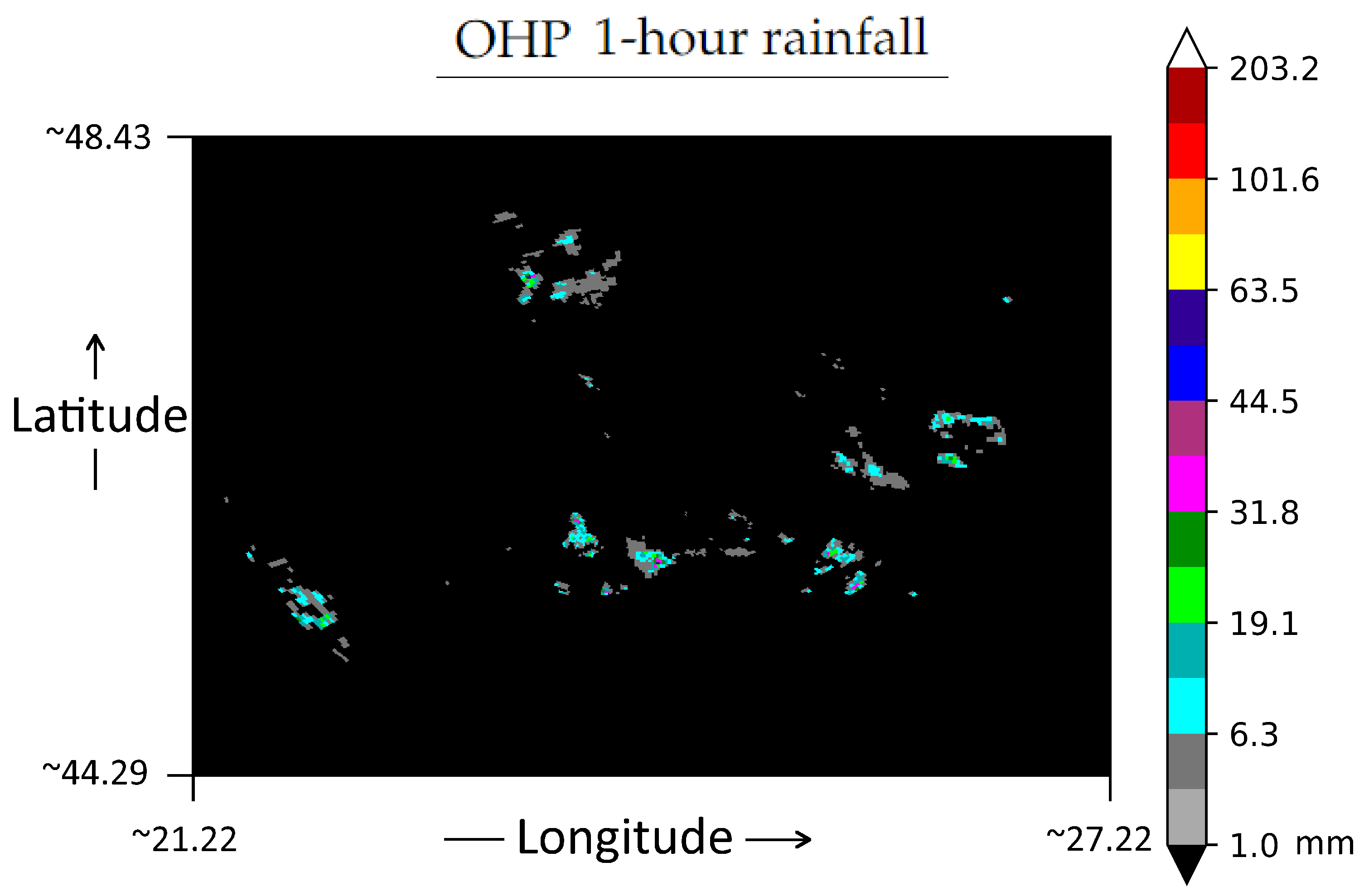
- How effective are the ML models designed to make estimations of the OHP using the reflectivity data on the first elevation levels?
- RQ3
- Do the stacked ML models bring a statistically significant performance improvement to QPE with respect to the performance of current operational baseline products?
2. Background
2.1. Literature Review on Precipitation Estimation and Nowcasting
2.2. Supervised Learning Models Used
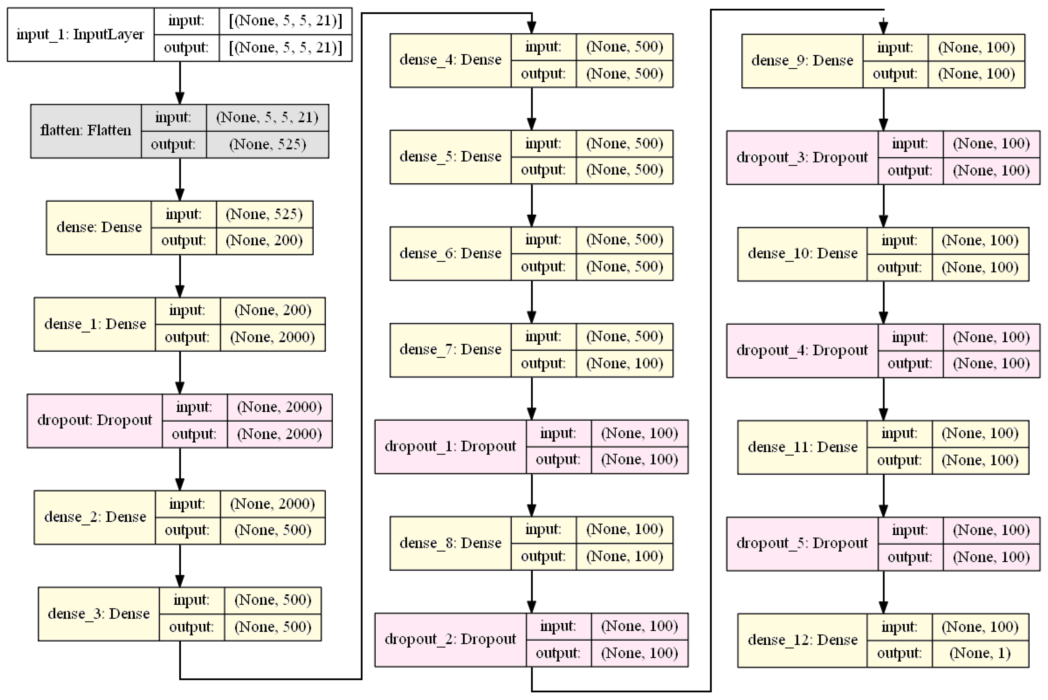
2.2.1. Deep Neural Networks
2.2.2. Support Vector Machines
2.2.3. Random Forests
2.2.4. k-Nearest Neighbors
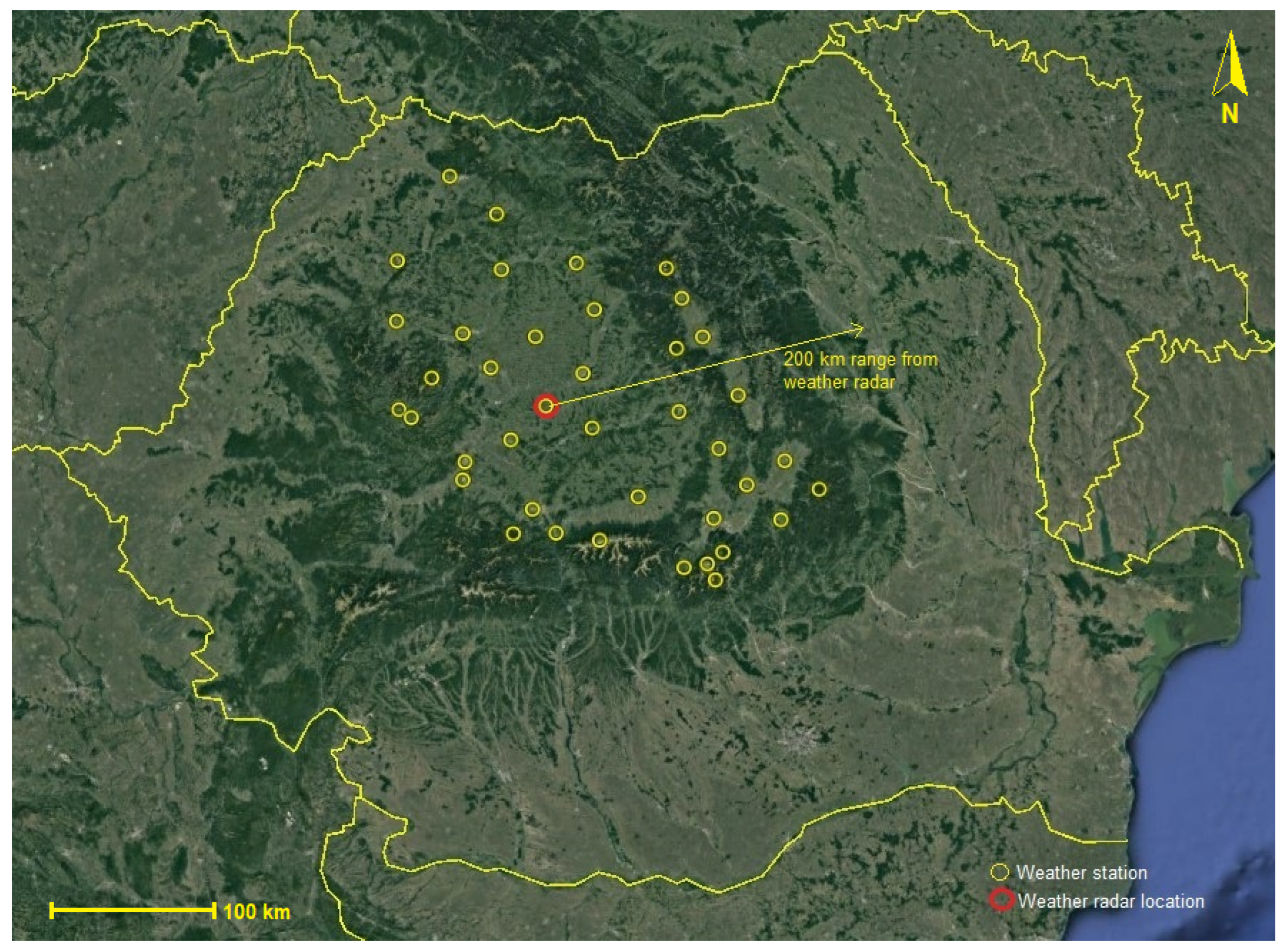
3. Data Set
3.1. Data Model
- -
- : the matrix coordinate to be computed (either i or j);
- -
- : the latitude or longitude of the weather station for which the matrix coordinates are computed (latitude is used for computing and longitude for );
- -
- : the latitude or longitude of the top-left corner of the data grid (latitude is used for computing and longitude for );
- -
- : real-world size of a data grid cell, measured in decimal degrees.
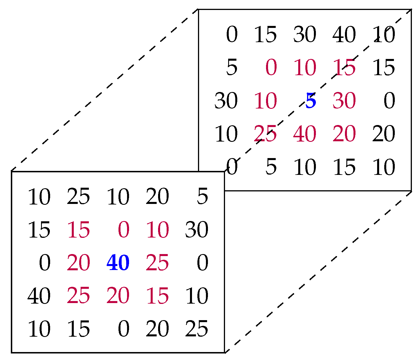
3.2. Data Representation
4. Methodology
4.1. Formalisation
4.2. ML Models Used
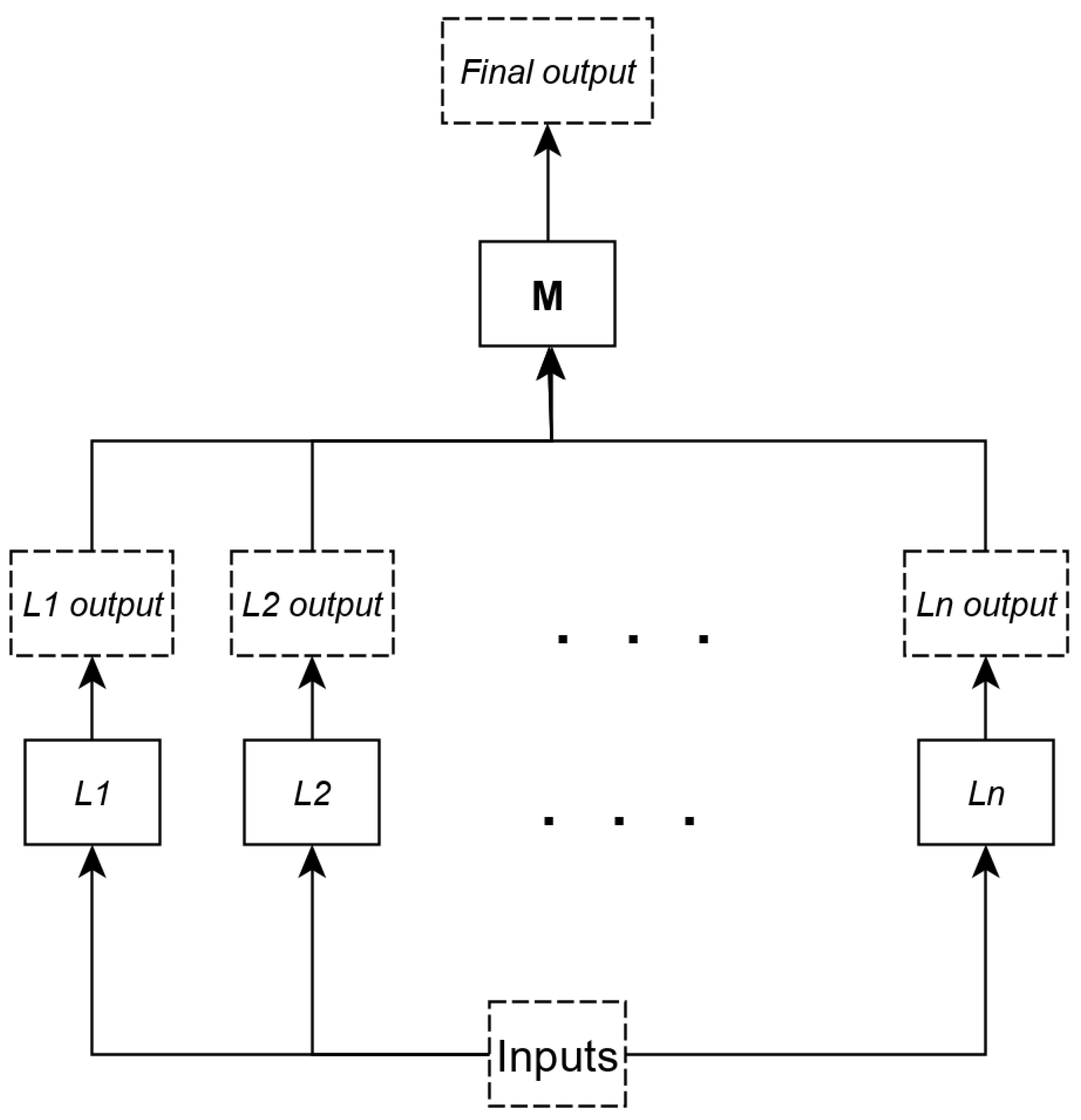
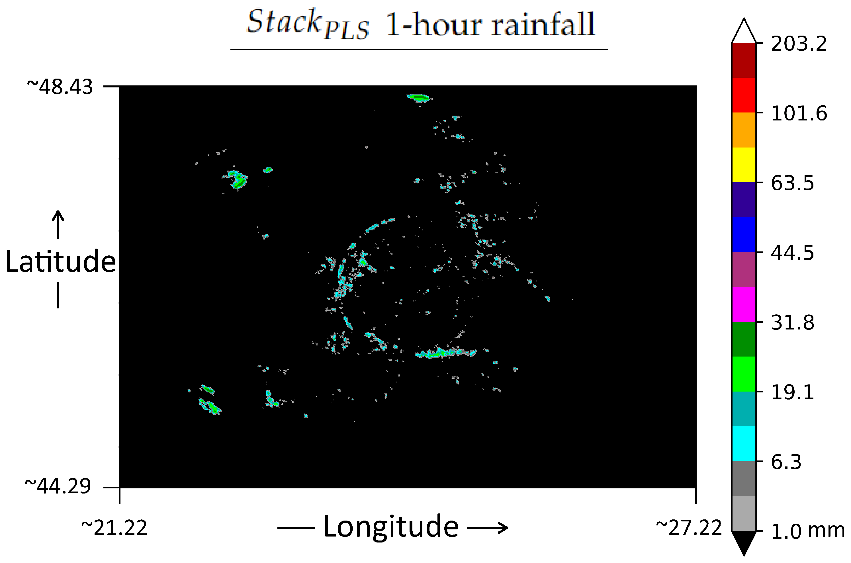
- A stacking model denoted by with base the DNN, SVM, kNN and RF regressors (i.e., and DNN, SVM, NN, RF) and in the top of the stack the Partial Least Squares (PLS) predictor ( PLS). The PLS regressor [51] is a variation of the linear least-square regression, where the model reduces the number of variables used for regression; it is especially useful for cases where instances have a high number of variables and there is a high chance that the variables are correlated.
- A stacking model denoted by with base the PLS, kNN and RF regressors (i.e., and PLS, NN, RF) and at the top of the stack our customized DNN predictor ( DNN).
4.3. Training
4.4. Testing and Performance Evaluation
4.4.1. Performance Metrics
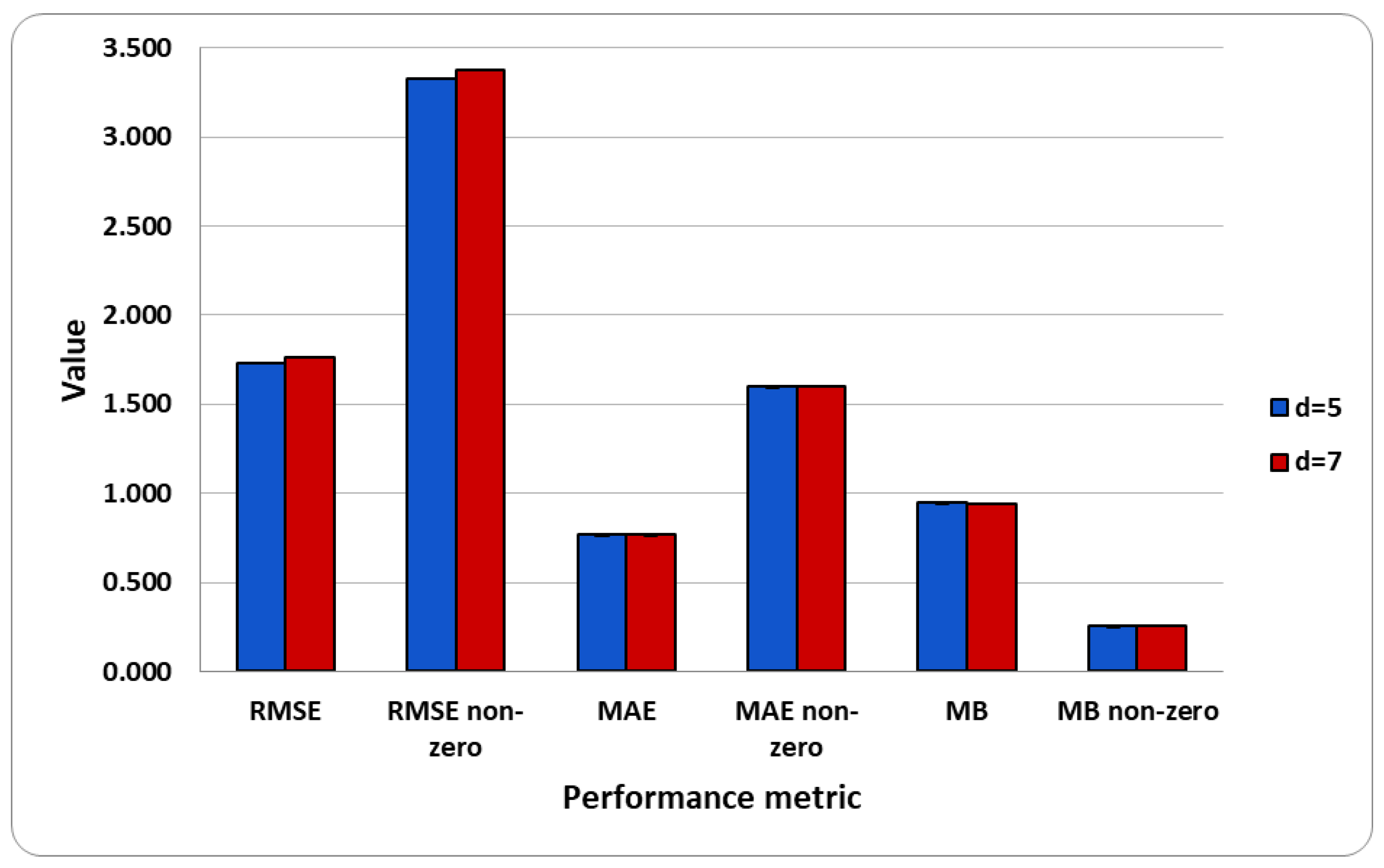
- Mean absolute error () computes the average of the absolute errors obtained for the testing instances: . Lower values for indicate better regressors.
- is used for computing the values only for the non zero-labeled testing instances (i.e., precipitations). This measure is particularly relevant, since we are particularly interested in our models being able to accurately estimate the precipitations (i.e., non-zero target outputs). Lower values for indicate smaller regression errors for the rainfall rate.
- Root mean squared error () computes the square root of the average of squared errors obtained for the testing instances: . Lower values for indicate better regressors.
- is used for computing the values only for the non zero-labeled testing instances. Lower values for indicate smaller regression errors for the precipitations.
- Multiplicative Bias () is used for comparing the average value of the forecast to the average value of the true observations: . expresses the degree of correspondence between the average forecast and the average observation, i.e., how many times the average prediction is bigger or lower than the average ground truth. The closer is to 1 the better.
- is used for computing the values only for the non zero-labeled testing instances (i.e., precipitations).
5. Results
5.1. Experimental Setup
5.2. Computational Results and Analysis
6. Discussion
6.1. Time Complexity Analysis
6.2. Comparison to Baselines
6.3. Comparison to Related Work
6.4. Interpretation from a Meteorological Perspective
6.5. Threats to Validity
7. Conclusions
Author Contributions
Funding
Institutional Review Board Statement
Informed Consent Statement
Data Availability Statement
Acknowledgments
Conflicts of Interest
References
- Wu, D.; Wu, L.; Zhang, T.; Zhang, W.; Huang, J.; Wang, X. Short-Term Rainfall Prediction Based on Radar Echo Using an Improved Self-Attention PredRNN Deep Learning Model. Atmosphere 2022, 13, 1963. [Google Scholar] [CrossRef]
- Bauer, H.S.; Schwitalla, T.; Wulfmeyer, V.; Bakhshaii, A.; Ehret, U.; Neuper, M.; Caumont, O. Quantitative precipitation estimation based on high-resolution numerical weather prediction and data assimilation with WRF—A performance test. Tellus A: Dyn. Meteorol. Oceanogr. 2015, 67, 25047. [Google Scholar] [CrossRef]
- Gleixner, S.; Demissie, T.; Diro, G.T. Did ERA5 Improve Temperature and Precipitation Reanalysis over East Africa? Atmosphere 2020, 11, 996. [Google Scholar] [CrossRef]
- Yang, D.; Elomaa, E.; Tuominen, A.; Aaltonen, A.; Goodison, B.; Gunther, T.; Golubev, V.; Sevruk, B.; Madsen, H.; Milkovic, J. Wind-induced Precipitation Undercatch of the Hellmann Gauges. Hydrol. Res. 1999, 30, 57–80. [Google Scholar] [CrossRef]
- Neuper, M.; Ehret, U. Quantitative precipitation estimation with weather radar using a data- and information-based approach. Hydrol. Earth Syst. Sci. 2019, 23, 3711–3733. [Google Scholar] [CrossRef] [Green Version]
- Thorndahl, S.; Einfalt, T.; Willems, P.; Nielsen, J.E.; ten Veldhuis, M.C.; Arnbjerg-Nielsen, K.; Rasmussen, M.R.; Molnar, P. Weather radar rainfall data in urban hydrology. Hydrol. Earth Syst. Sci. 2017, 21, 1359–1380. [Google Scholar] [CrossRef] [Green Version]
- Bronstert, A.; Ankit, A.; Berry, B.; Madlen, F.; Maik, H.; Lisei, K.R.; Thomas, M.; Dadiyorto, W. The Braunsbach Flashflood of May 29, 2016: A forensic analysis of the meteorological origin and the hydrological development an extreme hydro-meteorological event. In Proceedings of the EGU General Assembly Conference Abstracts, Vienna, Austria, 23–28 April 2017; p. 2942. [Google Scholar]
- Germann, U.; Galli, G.; Boscacci, M.; Bolliger, M. Radar precipitation measurement in a mountainous region. Q. J. R. Meteorol. Soc. 2006, 132, 1669–1692. [Google Scholar] [CrossRef]
- Overeem, A.; Holleman, I.; Buishand, A. Derivation of a 10-Year Radar-Based Climatology of Rainfall. J. Appl. Meteorol. Climatol. 2009, 48, 1448–1463. [Google Scholar] [CrossRef]
- Kronenberg, R.; Franke, J.; Bernhofer, C. Classification of daily precipitation patterns on the basis of radar-derived precipitation rates for Saxony, Germany. Meteorol. Z. 2012, 21, 475–486. [Google Scholar] [CrossRef]
- Alifujiang, Y.; Abuduwaili, J.; Maihemuti, B.; Emin, B.; Groll, M. Innovative Trend Analysis of Precipitation in the Lake Issyk-Kul Basin, Kyrgyzstan. Atmosphere 2020, 11, 332. [Google Scholar] [CrossRef]
- Goudenhoofdt, E.; Delobbe, L.; Willems, P. Regional frequency analysis of extreme rainfall in Belgium based on radar estimates. Hydrol. Earth Syst. Sci. 2017, 21, 5385–5399. [Google Scholar] [CrossRef] [Green Version]
- Fulton, R.A.; Breidenbach, J.P.; Seo, D.J.; Miller, D.A.; O’Bannon, T. The WSR-88D Rainfall Algorithm. Weather. Forecast. 1998, 13, 377–395. [Google Scholar] [CrossRef]
- Tian, W.; Yi, L.; Liu, W.; Huang, W.; Ma, G.; Zhang, Y. Ground Radar Precipitation Estimation with Deep Learning Approaches in Meteorological Private Cloud. J. Cloud Comput. 2020, 9, 1–12. [Google Scholar] [CrossRef] [Green Version]
- Huffman, G.J.; Adler, R.F.; Bolvin, D.T.; Gu, G.; Nelkin, E.J.; Bowman, K.P.; Hong, Y.; Stocker, E.F.; Wolff, D.B. The TRMM Multisatellite Precipitation Analysis (TMPA): Quasi-Global, Multiyear, Combined-Sensor Precipitation Estimates at Fine Scales. J. Hydrometeorol. 2006, 8, 38–55. [Google Scholar] [CrossRef]
- Skofronick-Jackson, G.; Petersen, W.A.; Berg, W.; Kidd, C.; Stocker, E.F.; Kirschbaum, D.B.; Kakar, R.; Braun, S.A.; Huffman, G.J.; Iguchi, T.; et al. The Global Precipitation Measurement (GPM) Mission for Science and Society. Bull. Am. Meteorol. Soc. 2017, 98, 1679–1695. [Google Scholar] [CrossRef] [PubMed]
- Tan, A.; Nasa, G.J.H.; Bolvin, D.T.; Nelkin, E.J. IMERG V06: Changes to the Morphing Algorithm. Am. Meteorol. Soc. 2019, 36, 2471–2482. [Google Scholar] [CrossRef]
- Zhang, J.; Howard, K.; Langston, C.; Vasiloff, S.; Kaney, B.; Arthur, A.; Cooten, S.V.; Kelleher, K.; Kitzmiller, D.; Ding, F.; et al. National Mosaic and Multi-Sensor QPE (NMQ) System: Description, Results, and Future Plans. Bull. Am. Meteorol. Soc. 2011, 92, 1321–1338. [Google Scholar] [CrossRef] [Green Version]
- Zhang, J.; Howard, K.; Langston, C.; Kaney, B.; Qi, Y.; Tang, L.; Grams, H.; Wang, Y.; Cocks, S.; Martinaitis, S.; et al. Multi-Radar Multi-Sensor (MRMS) Quantitative Precipitation Estimation: Initial Operating Capabilities. Bull. Am. Meteorol. Soc. 2016, 97, 621–638. [Google Scholar] [CrossRef]
- Zhang, J.; Tang, L.; Cocks, S.; Zhang, P.; Ryzhkov, A.; Howard, K.; Langston, C.; Kaney, B. A Dual-Polarization Radar Synthetic QPE for Operations. J. Hydrometeorol. 2020, 21, 2507–2521. [Google Scholar] [CrossRef] [Green Version]
- Yang, J.; Xiang, Y.; Sun, J.; Xu, X. Multi-Model Ensemble Prediction of Summer Precipitation in China Based on Machine Learning Algorithms. Atmosphere 2022, 13, 1424. [Google Scholar] [CrossRef]
- Marzuki; Hashiguchi, H.; Vonnisa, M.; Harmadi; Muzirwan; Nugroho, S.; Yoseva, M. Z-R Relationships for Weather Radar in Indonesia from the Particle Size and Velocity (Parsivel) Optical Disdrometer. In Proceedings of the 2018 Progress in Electromagnetics Research Symposium (PIERS-Toyama), Toyama, Japan, 1–4 August 2018; pp. 37–41. [Google Scholar]
- Jeworrek, J.; West, G.; Stull, R. Optimizing Analog Ensembles for Sub-Daily Precipitation Forecasts. Atmosphere 2022, 13, 1662. [Google Scholar] [CrossRef]
- Perez, G.M.P. Improving the Quantitative Precipitation Forecast: A Deep Learning Approach. Ph.D. Thesis, University of Sao Paulo, Institute of Astronomy, Geophysics and Atmospheric Sciences, Department of Atmospheric Sciences, São Paulo, Brazil, 2018. [Google Scholar]
- Ridwan, W.M.; Sapitang, M.; Aziz, A.; Kushiar, K.F.; Ahmed, A.N.; El-Shafie, A. Rainfall forecasting model using machine learning methods: Case study Terengganu, Malaysia. Ain Shams Eng. J. 2021, 12, 1651–1663. [Google Scholar] [CrossRef]
- Sun, D.; Wu, J.; Huang, H.; Wang, R.; Liang, F.; Xinhua, H. Prediction of Short-Time Rainfall Based on Deep Learning. Math. Probl. Eng. 2021, 2021, 6664413. [Google Scholar] [CrossRef]
- Zhang, F.; Wang, X.; Guan, J. A Novel Multi-Input Multi-Output Recurrent Neural Network Based on Multimodal Fusion and Spatiotemporal Prediction for 0–4 Hour Precipitation Nowcasting. Atmosphere 2021, 12, 1596. [Google Scholar] [CrossRef]
- Yo, T.S.; Su, S.H.; Chu, J.L.; Chang, C.W.; Kuo, H.C. A Deep Learning Approach to Radar-Based QPE. Earth Space Sci. 2021, 8, e2020EA001340. [Google Scholar] [CrossRef]
- AmeriGEOSS. Weather Radar Base Reflectivity Mosaic. Available online: https://data.amerigeoss.org/dataset/weather-radar-base-reflectivity-mosaic1 (accessed on 15 May 2021).
- Trömel, S.; Chwala, C.; Furusho-Percot, C.; Henken, C.C.; Polz, J.; Potthast, R.; Reinoso-Rondinel, R.; Simmer, C. Near-Realtime Quantitative Precipitation Estimation and Prediction (RealPEP). Bull. Am. Meteorol. Soc. 2021, 102, E1591–E1596. [Google Scholar] [CrossRef]
- Chen, J.Y.; Trömel, S.; Ryzhkov, A.; Simmer, C. Assessing the Benefits of Specific Attenuation for Quantitative Precipitation Estimation with a C-Band Radar Network. J. Hydrometeorol. 2021, 22, 2617–2631. [Google Scholar] [CrossRef]
- Shin, K.; Song, J.J.; Bang, W.; Lee, G. Quantitative Precipitation Estimates Using Machine Learning Approaches with Operational Dual-Polarization Radar Data. Remote Sens. 2021, 13, 694. [Google Scholar] [CrossRef]
- Moraux, A.; Dewitte, S.; Cornelis, B.; Munteanu, A. A Deep Learning Multimodal Method for Precipitation Estimation. Remote Sens. 2021, 13, 3278. [Google Scholar] [CrossRef]
- Ko, J.; Lee, K.; Hwang, H.; Oh, S.G.; Son, S.W.; Shin, K. Effective training strategies for deep-learning-based precipitation nowcasting and estimation. Comput. Geosci. 2022, 161, 105072. [Google Scholar] [CrossRef]
- Mitchell, T.M. Machine Learning, 1st ed.; McGraw-Hill, Inc.: New York, NY, USA, 1997. [Google Scholar]
- Goodfellow, I.; Bengio, Y.; Courville, A. Deep Learning; MIT Press: Cambridge, MA, USA, 2016. [Google Scholar]
- Srivastava, N.; Hinton, G.E.; Krizhevsky, A.; Sutskever, I.; Salakhutdinov, R. Dropout: A simple way to prevent neural networks from overfitting. J. Mach. Learn. Res. 2014, 15, 1929–1958. [Google Scholar]
- Nowlan, S.J.; Hinton, G.E. Simplifying Neural Networks by Soft Weight-Sharing. Neural Comput. 1992, 4, 473–493. [Google Scholar] [CrossRef]
- Cortes, C.; Vapnik, V. Support-vector networks. Mach. Learn. 1995, 20, 273–297. [Google Scholar] [CrossRef]
- Pisner, D.A.; Schnyer, D.M. Chapter 6-Support vector machine. In Machine Learning; Mechelli, A., Vieira, S., Eds.; Academic Press: Cambridge, MA, USA, 2020; pp. 101–121. [Google Scholar]
- Smola, A.; Schölkopf, B. A tutorial on support vector regression. Stat. Comput. 2004, 14, 199–222. [Google Scholar] [CrossRef] [Green Version]
- Biau, G.; Scornet, E.; Welbl, J. Neural Random Forests. Sankhya A 2019, 81, 347–386. [Google Scholar] [CrossRef]
- Sun, B.; Chen, H. A Survey of Nearest Neighbor Algorithms for Solving the Class Imbalanced Problem. Wirel. Commun. Mob. Comput. 2021, 2021, 5520990. [Google Scholar] [CrossRef]
- Tang, B.; He, H. A local density-based approach for outlier detection. Neurocomputing 2017, 241, 171–180. [Google Scholar] [CrossRef] [Green Version]
- Salvador–Meneses, J.; Ruiz–Chavez, Z.; Garcia–Rodriguez, J. Compressed kNN: K-Nearest Neighbors with Data Compression. Entropy 2019, 21, 234. [Google Scholar] [CrossRef] [Green Version]
- Mihai, A. Radar and Rainfall Data Sets. Available online: https://zenodo.org/record/7086999 (accessed on 1 December 2021).
- SciPy. Fundamental Algorithms for Scientific Computing in Python. Available online: https://scipy.org/ (accessed on 10 December 2021).
- Liang, M.; Chang, T.; An, B.; Duan, X.; Du, L.; Wang, X.; Miao, J.; Xu, L.; Gao, X.; Zhang, L.; et al. A Stacking Ensemble Learning Framework for Genomic Prediction. Front. Genet. 2021, 12, 600040. [Google Scholar] [CrossRef]
- Zhou, Z.H. Ensemble Learning. In Encyclopedia of Biometrics; Springer: Boston, MA, USA, 2009; pp. 270–273. [Google Scholar]
- Wolpert, D.H. Stacked generalization. Neural Netw. 1992, 5, 241–259. [Google Scholar] [CrossRef]
- Manthey, L.; Ousley, S.D. Chapter 5.3-Geometric morphometrics. In Statistics and Probability in Forensic Anthropology; Academic Press: Cambridge, MA, USA, 2020; pp. 289–298. [Google Scholar]
- Boehmke, B.C.; Greenwell, B.M. Hands-On Machine Learning with R-Chapter 5; Taylor & Francis: New York, NY, USA, 2019. [Google Scholar]
- Online Scikit-Learn API Documentation. Available online: https://scikit-learn.org/stable/modules/classes.html (accessed on 1 August 2022).
- Simundic, A.M. Confidence interval. Biochem. Medica 2008, 18, 154–161. [Google Scholar] [CrossRef]
- Kingma, D.P.; Ba, J. Adam: A Method for Stochastic Optimization. In Proceedings of the 3rd International Conference on Learning Representations, ICLR 2015, San Diego, CA, USA, 7–9 May 2015; Bengio, Y., LeCun, Y., Eds.; 2015; pp. 1–15. [Google Scholar]
- Siegel, S.; Castellan, N. Nonparametric Statistics for the Behavioral Sciences, 2nd ed.; McGraw–Hill, Inc.: New York, NY, USA, 1988. [Google Scholar]
- Online Web Statistical Calculators. Available online: https://astatsa.com/WilcoxonTest/ (accessed on 15 May 2022).
- Dumitrescu, A.; Brabec, M.; Matreata, M. Integrating Ground-based Observations and Radar Data Into Gridding Sub-daily Precipitation. Water Resour. Manag. 2020, 34, 3479–3497. [Google Scholar] [CrossRef]
- Runeson, P.; Höst, M. Guidelines for Conducting and Reporting Case Study Research in Software Engineering. Empir. Softw. Engg. 2009, 14, 131–164. [Google Scholar] [CrossRef] [Green Version]
- Su, Y.; Zhao, C.; Wang, Y.; Ma, Z. Spatiotemporal Variations of Precipitation in China Using Surface Gauge Observations from 1961 to 2016. Atmosphere 2020, 11, 303. [Google Scholar] [CrossRef]


| Metric | d | DNN | SVM | kNN | RF | ||
|---|---|---|---|---|---|---|---|
| 3 | 2.065 ± 0.058 | 1.774 ± 0.06 | 1.943 ± 0.107 | 1.813 ± 0.055 | 1.734 ± 0.06 | 2.085 ± 0.1 | |
| 5 | 2.045 ± 0.053 | 1.774 ± 0.06 | 1.891 ± 0.055 | 1.818 ± 0.051 | 1.734 ± 0.059 | 2.027 ± 0.079 | |
| 7 | 2.004 ± 0.034 | 1.774 ± 0.06 | 1.907 ± 0.047 | 1.827 ± 0.044 | 1.764 ± 0.046 | 2.028 ± 0.083 | |
| 3 | 3.16 ± 0.165 | 3.507 ± 0.106 | 3.422 ± 0.112 | 3.321 ± 0.109 | 3.328 ± 0.11 | 3.106 ± 0.118 | |
| 5 | 3.167 ± 0.164 | 3.507 ± 0.106 | 3.424 ± 0.102 | 3.303 ± 0.113 | 3.328 ± 0.11 | 3.107 ± 0.112 | |
| 7 | 3.107 ± 0.105 | 3.507 ± 0.106 | 3.428 ± 0.094 | 3.302 ± 0.1 | 3.376 ± 0.074 | 3.123 ± 0.127 | |
| 3 | 1.55 ± 0.057 | 0.535 ± 0.01 | 0.833 ± 0.053 | 0.863 ± 0.014 | 0.766 ± 0.022 | 1.500 ± 0.11 | |
| 5 | 1.512 ± 0.038 | 0.535 ± 0.01 | 0.786 ± 0.022 | 0.896 ± 0.008 | 0.766 ± 0.022 | 1.435 ± 0.079 | |
| 7 | 1.473 ± 0.034 | 0.535 ± 0.01 | 0.81 ± 0.032 | 0.908 ± 0.009 | 0.768 ± 0.023 | 1.406 ± 0.087 | |
| 3 | 1.684 ± 0.04 | 1.804 ± 0.032 | 1.783 ± 0.052 | 1.631 ± 0.028 | 1.595 ± 0.027 | 1.673 ± 0.053 | |
| 5 | 1.672 ± 0.038 | 1.804 ± 0.032 | 1.778 ± 0.025 | 1.630 ± 0.031 | 1.596 ± 0.027 | 1.643 ± 0.037 | |
| 7 | 1.624 ± 0.042 | 2.218 ± 0.516 | 2.419 ± 0.791 | 1.916 ± 0.583 | 1.601 ± 0.024 | 1.638 ± 0.042 | |
| 3 | 3.065 ± 0.135 | 0.206 ± 0.005 | 1.127 ± 0.047 | 1.236 ± 0.057 | 0.945 ± 0.017 | 2.973 ± 0.280 | |
| 5 | 2.971 ± 0.125 | 0.206 ± 0.005 | 0.898 ± 0.048 | 1.329 ± 0.056 | 0.946 ± 0.02 | 2.81 ± 0.208 | |
| 7 | 2.876 ± 0.121 | 0.206 ± 0.005 | 0.909 ± 0.054 | 1.364 ± 0.055 | 0.940 ± 0.022 | 2.736 ± 0.229 | |
| 3 | 0.774±0.037 | 0.053 ± 0.001 | 0.266 ± 0.033 | 0.314 ± 0.014 | 0.254 ± 0.012 | 0.759 ± 0.069 | |
| 5 | 0.750 ± 0.033 | 0.053 ± 0.001 | 0.236 ± 0.019 | 0.339 ± 0.014 | 0.253 ± 0.013 | 0.713 ± 0.049 | |
| 7 | 0.731 ± 0.032 | 0.053 ± 0.001 | 0.253 ± 0.025 | 0.349 ± 0.015 | 0.256 ± 0.017 | 0.696 ± 0.055 |
| d | DNN | SVM | kNN | RF | ||
|---|---|---|---|---|---|---|
| 3 | 13 | 9 | 14 | 18 | 22 | 15 |
| 5 | 12 | 9 | 13 | 18 | 23 | 16 |
| 7 | 16 | 10 | 13 | 17 | 23 | 14 |
| 41 | 28 | 40 | 53 | 68 | 45 |
| Stage | DNN | SVR | kNN | RF | PLS | ||
|---|---|---|---|---|---|---|---|
| Training | 8673 ± 113 | 66.9 ± 1.15 | 0.01 ± 0.00 | 138 ± 10.8 | 0.23 ± 0.00 | 13.4 ± 0.67 | 1330 ± 16.8 |
| Testing | 0.52 ± 0.02 | 34.9 ± 0.99 | 4.40 ± 0.17 | 0.25 ± 0.01 | 0.03 ± 0.00 | 5.03 ± 0.10 | 3.28 ± 0.18 |
| ML Model/Baseline | RMSE | MAE | MB | |||
|---|---|---|---|---|---|---|
| with | 1.734 ± 0.059 | 3.328 ± 0.11 | 0.766 ± 0.022 | 1.596 ± 0.027 | 0.946 ± 0.02 | 0.253 ± 0.013 |
| OHP | 2.60 ± 0.334 | 4.507 ± 0.781 | 0.657 ± 0.082 | 2.349 ± 0.310 | 0.694 ± 0.166 | 0.280 ± 0.107 |
| ZR | 2.012 ± 0.067 | 3.625 ± 0.138 | 0.608 ± 0.012 | 1.882 ± 0.047 | 0.430 ± 0.01 | 0.170 ± 0.008 |
Disclaimer/Publisher’s Note: The statements, opinions and data contained in all publications are solely those of the individual author(s) and contributor(s) and not of MDPI and/or the editor(s). MDPI and/or the editor(s) disclaim responsibility for any injury to people or property resulting from any ideas, methods, instructions or products referred to in the content. |
© 2023 by the authors. Licensee MDPI, Basel, Switzerland. This article is an open access article distributed under the terms and conditions of the Creative Commons Attribution (CC BY) license (https://creativecommons.org/licenses/by/4.0/).
Share and Cite
Mihuleţ, E.; Burcea, S.; Mihai, A.; Czibula, G. Enhancing the Performance of Quantitative Precipitation Estimation Using Ensemble of Machine Learning Models Applied on Weather Radar Data. Atmosphere 2023, 14, 182. https://doi.org/10.3390/atmos14010182
Mihuleţ E, Burcea S, Mihai A, Czibula G. Enhancing the Performance of Quantitative Precipitation Estimation Using Ensemble of Machine Learning Models Applied on Weather Radar Data. Atmosphere. 2023; 14(1):182. https://doi.org/10.3390/atmos14010182
Chicago/Turabian StyleMihuleţ, Eugen, Sorin Burcea, Andrei Mihai, and Gabriela Czibula. 2023. "Enhancing the Performance of Quantitative Precipitation Estimation Using Ensemble of Machine Learning Models Applied on Weather Radar Data" Atmosphere 14, no. 1: 182. https://doi.org/10.3390/atmos14010182