

Deep Learning-Based Univariate Prediction of Daily Rainfall: Application to a Flood-Prone, Data-Deficient Country

 ,
,
Abstract
:1. Introduction
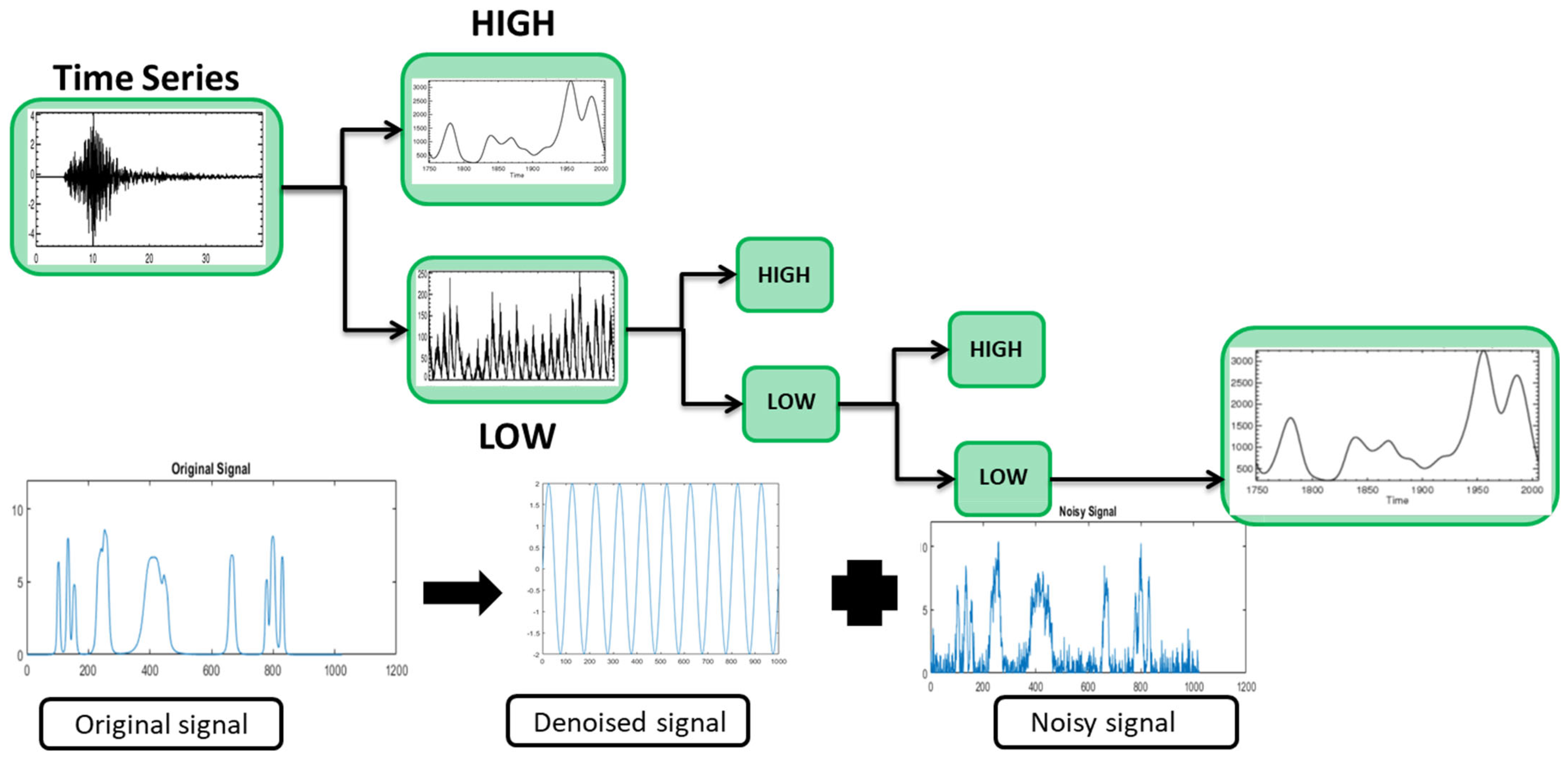
2. Discrete Wavelet Transform
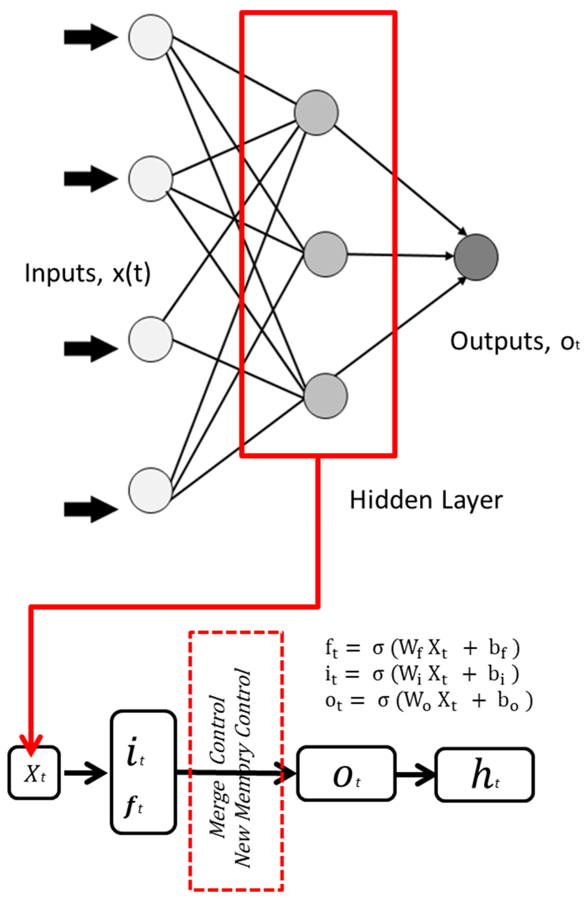
3. Long Short-Term Memory Network
4. Model Performance Indicators
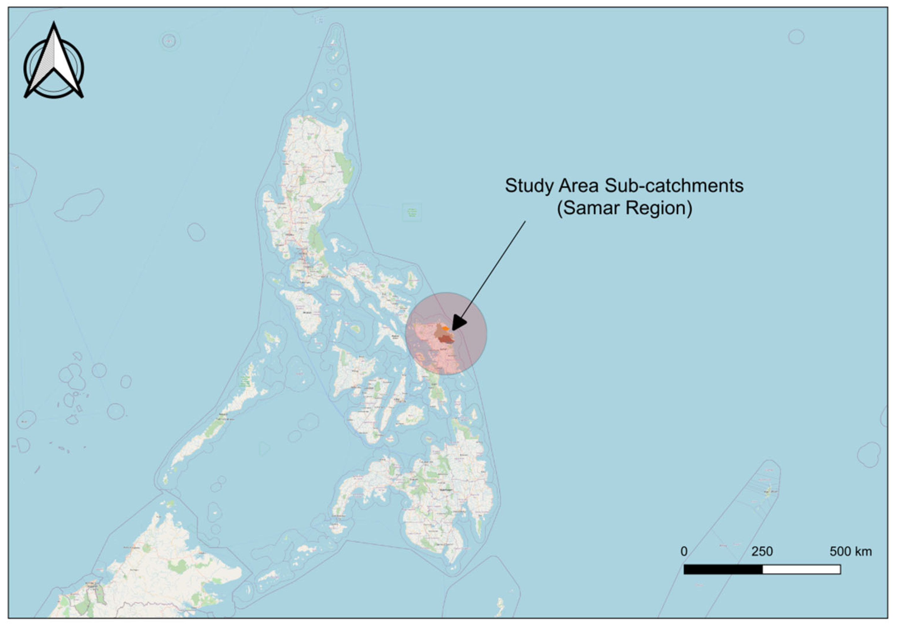
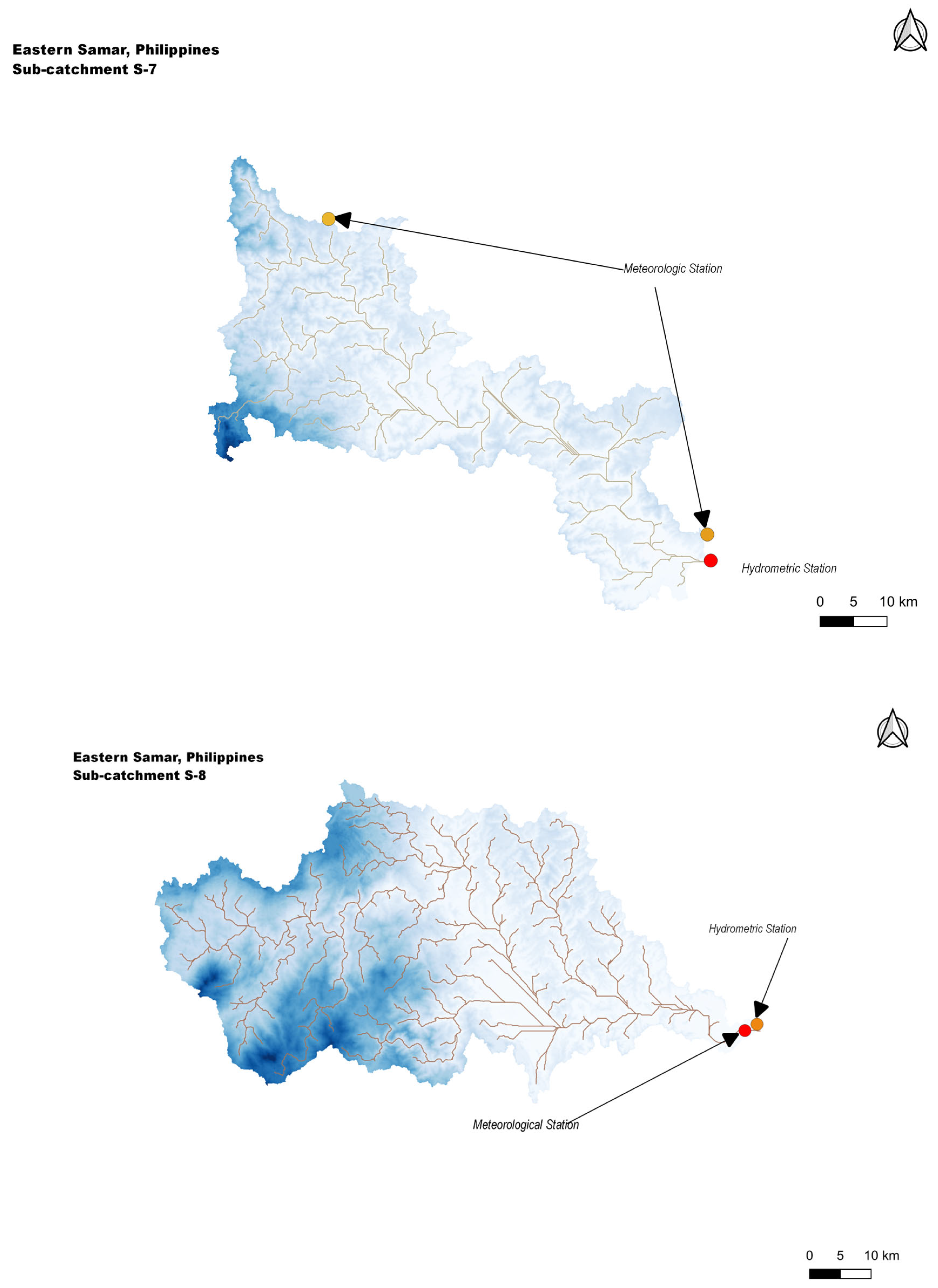
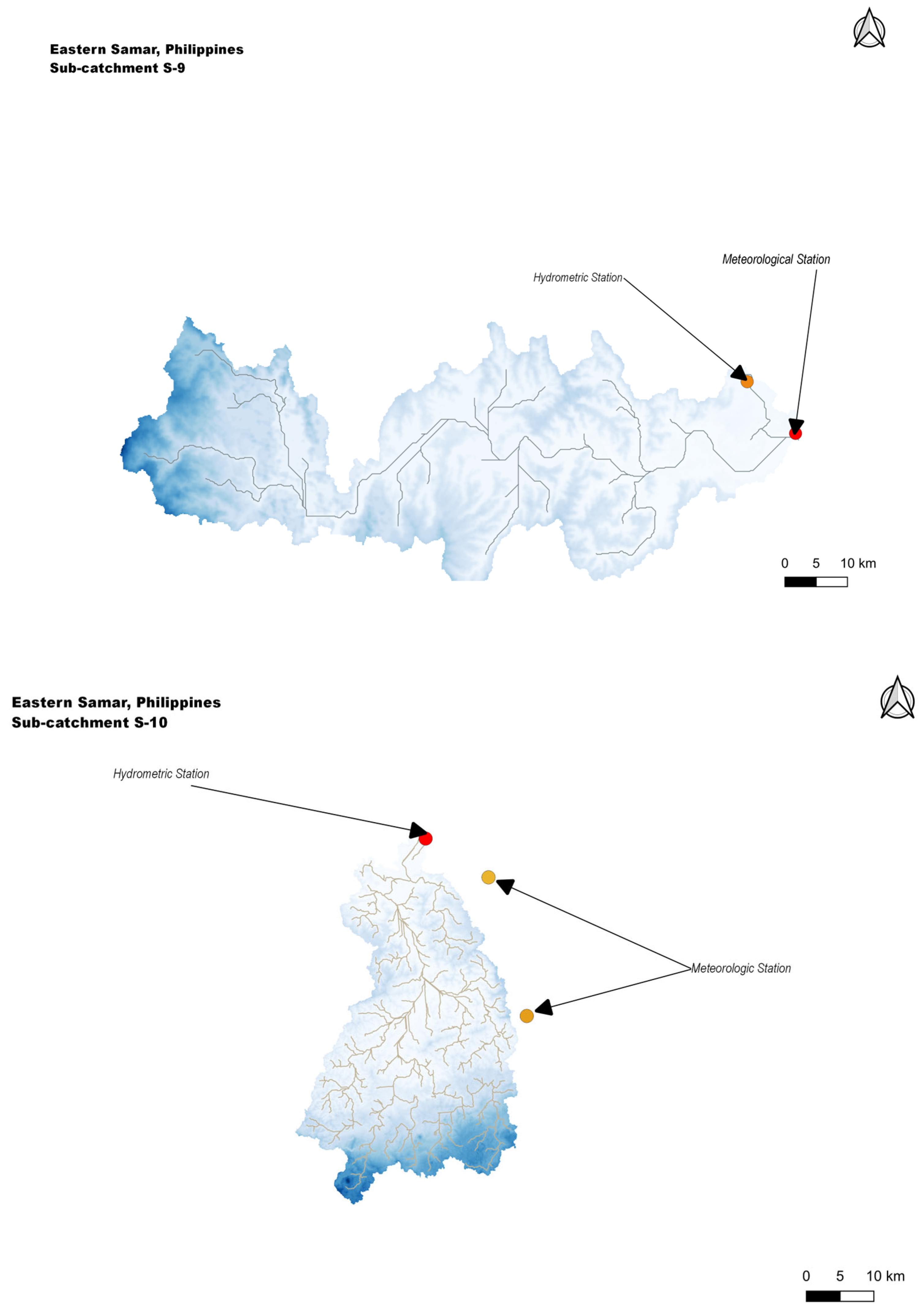
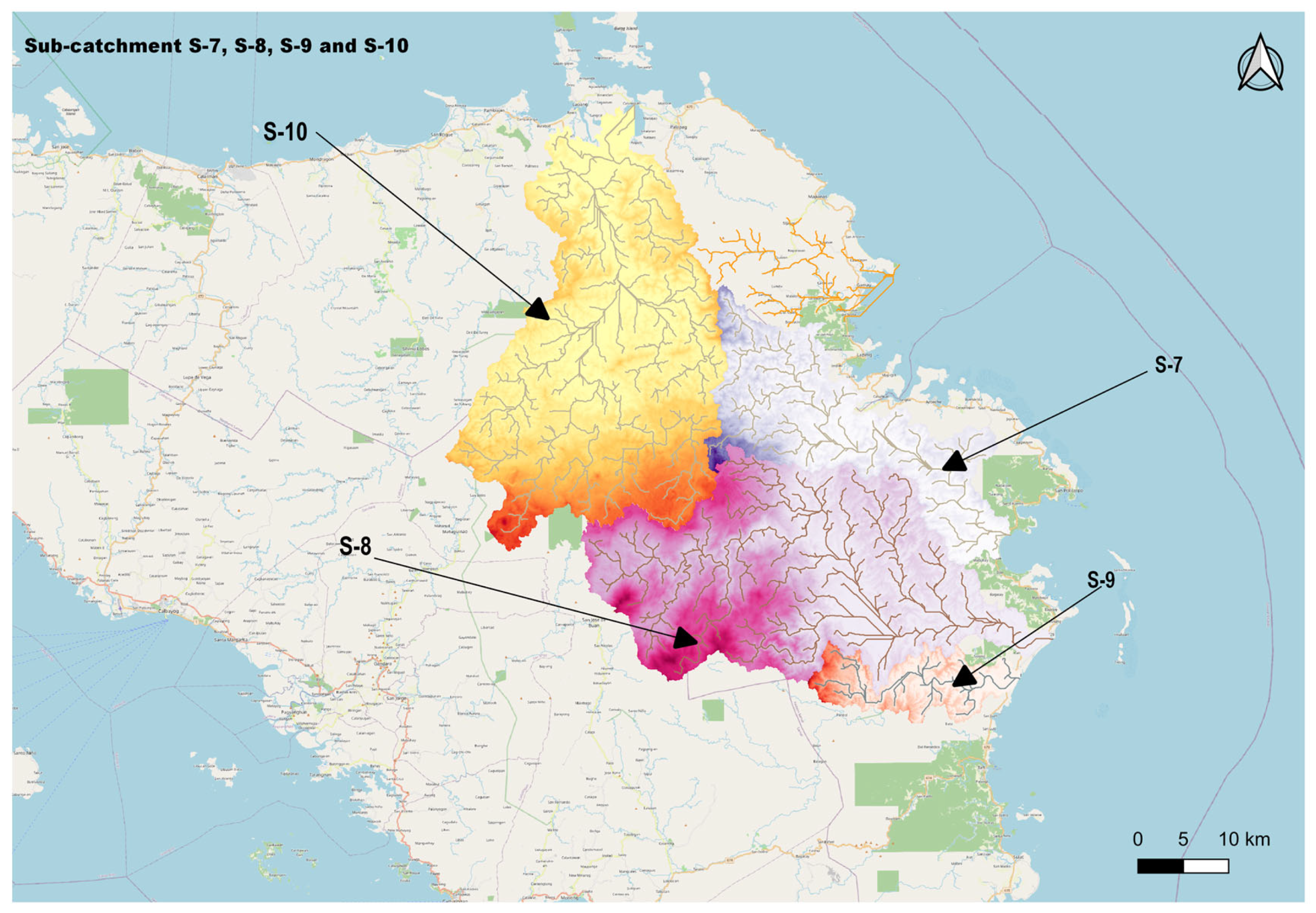
5. Study Area

| Subcatchment Name | Station Number | From | To |
|---|---|---|---|
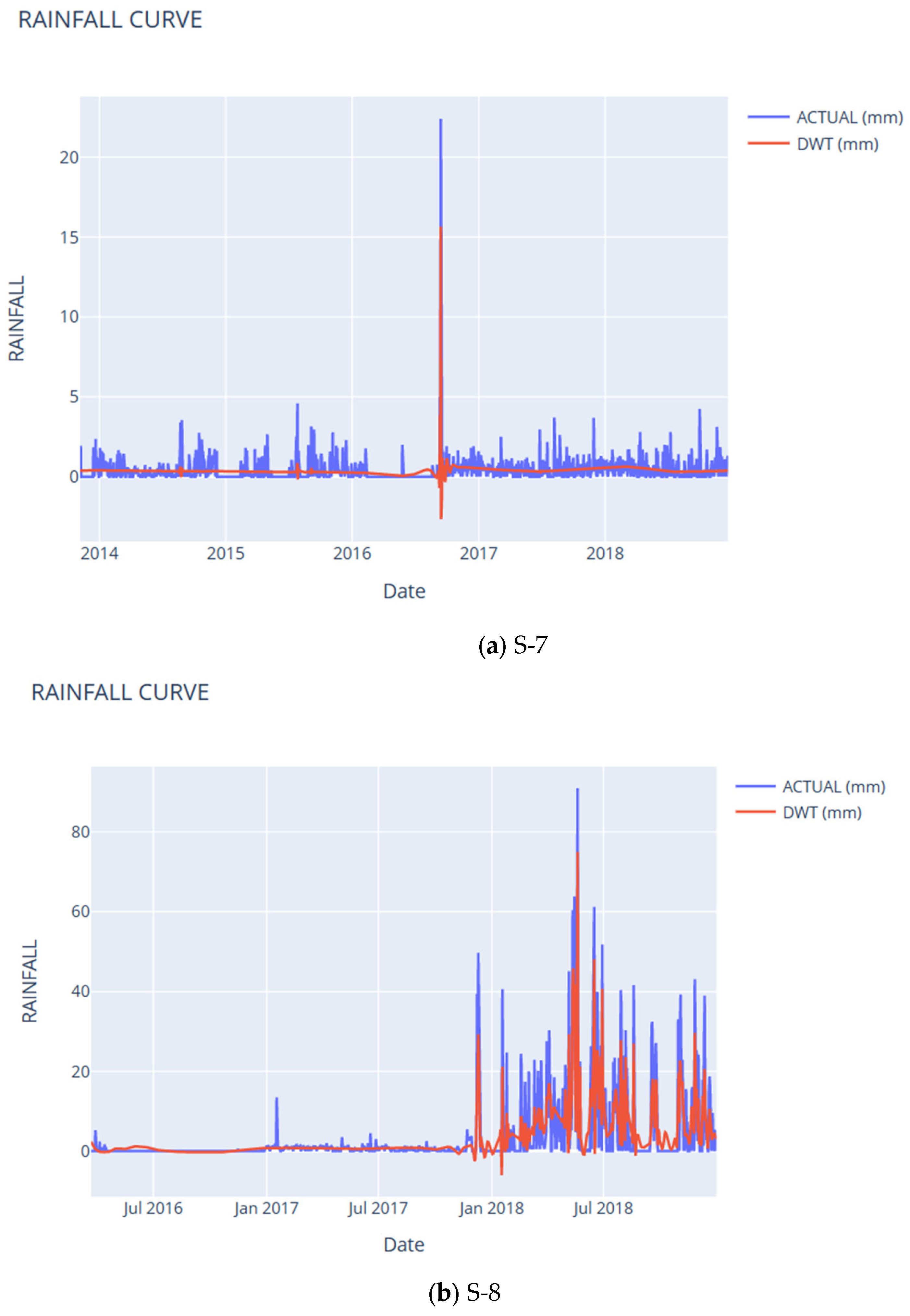
| S-7 (Oras) | 1155 | 6 November 2013 | 22 December 2018 |
| S-8 (Dolores) | 1767 | 22 March 2016 | 31 December 2018 |
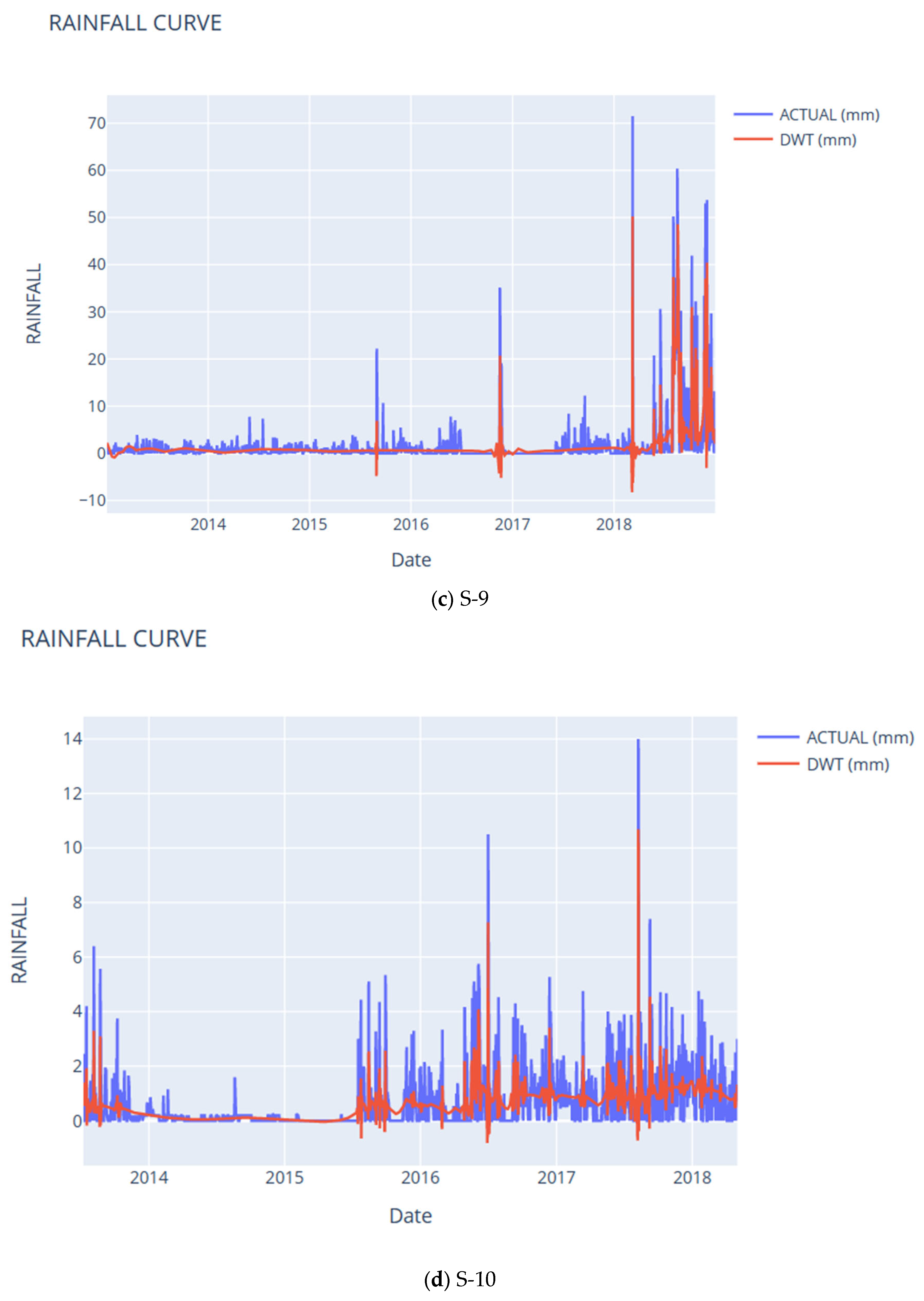
| S-9 (Can-avid) | 93 | 2 January 2013 | 31 December 2018 |
| S-10 (Catubig) | 547 | 9 July 2013 | 2 May 2018 |
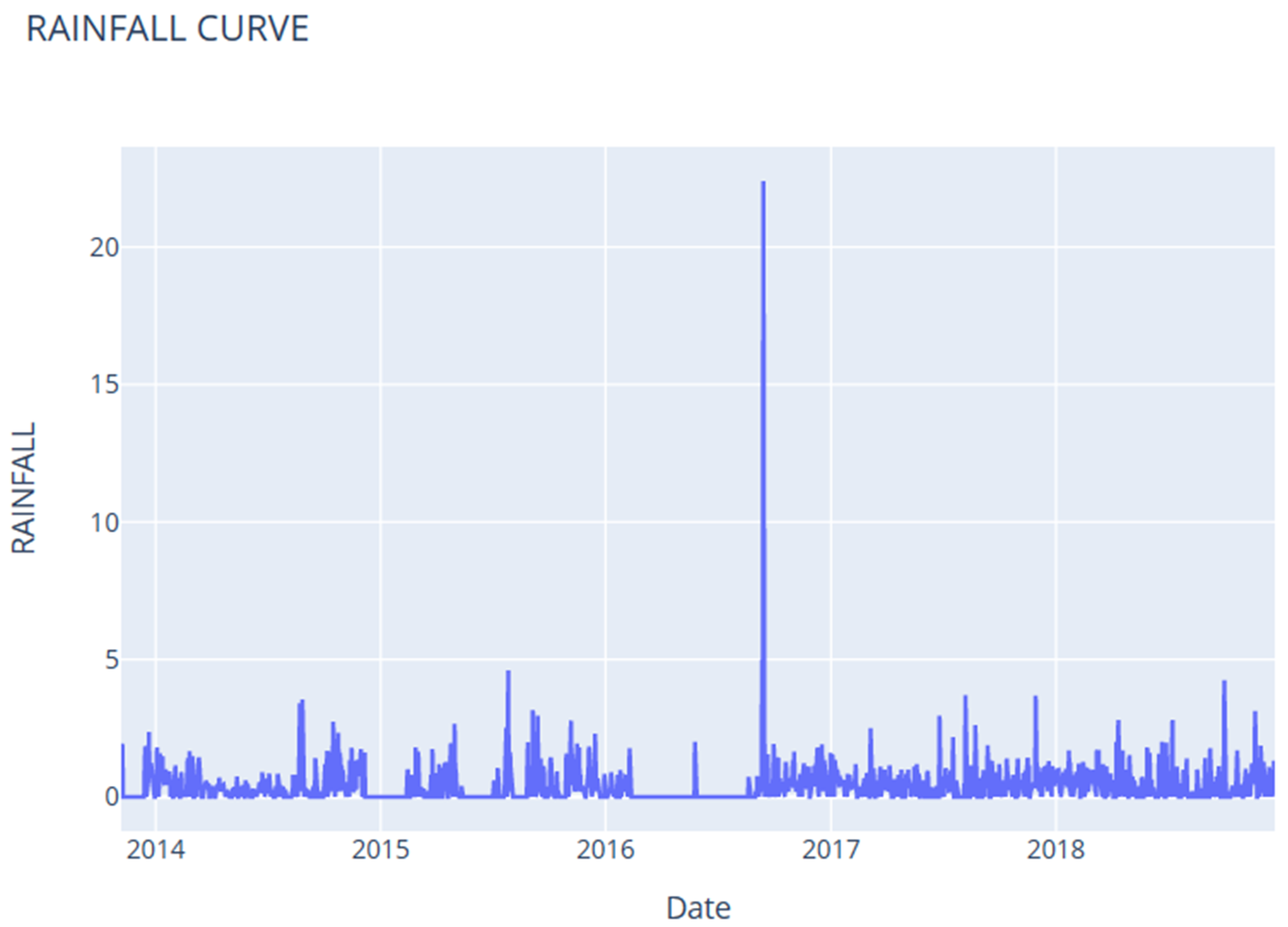
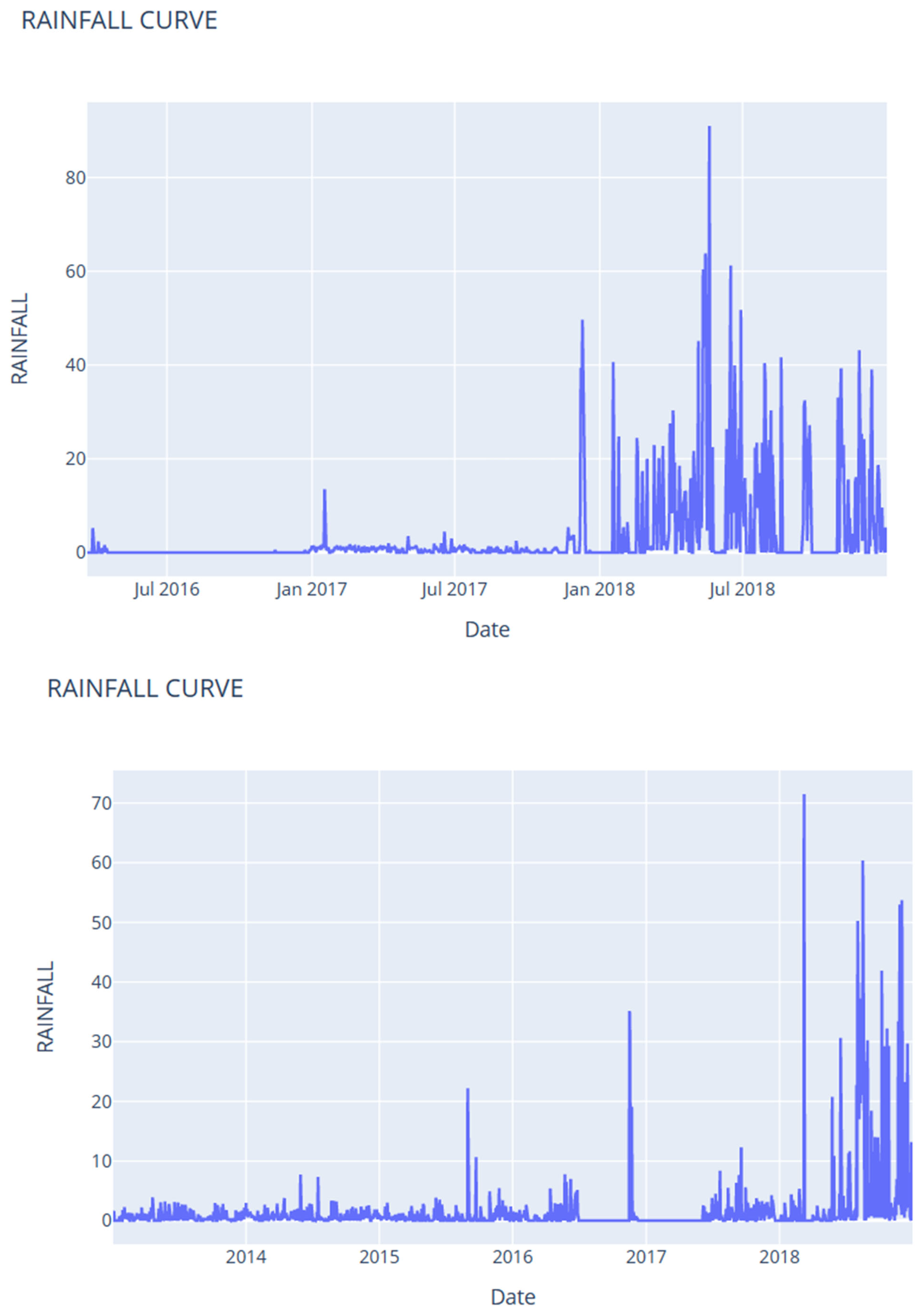
6. Data Collection and Characteristics
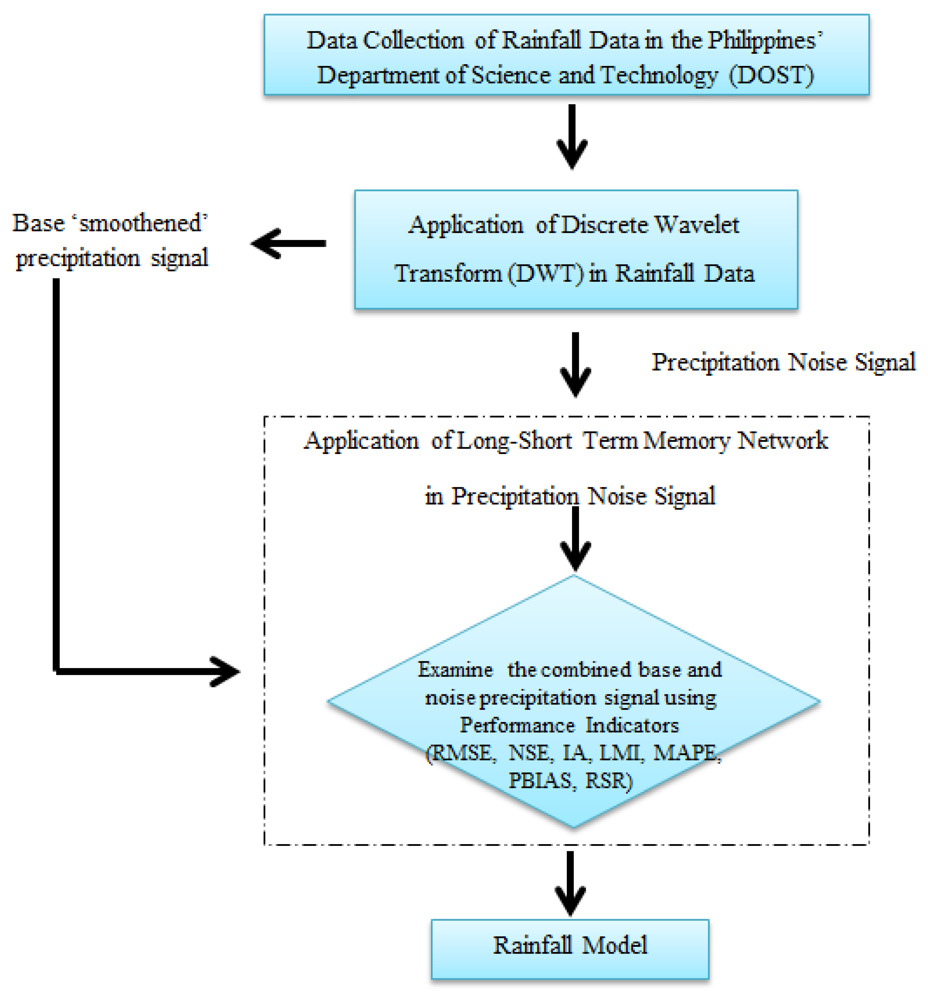
7. Overview of the Process
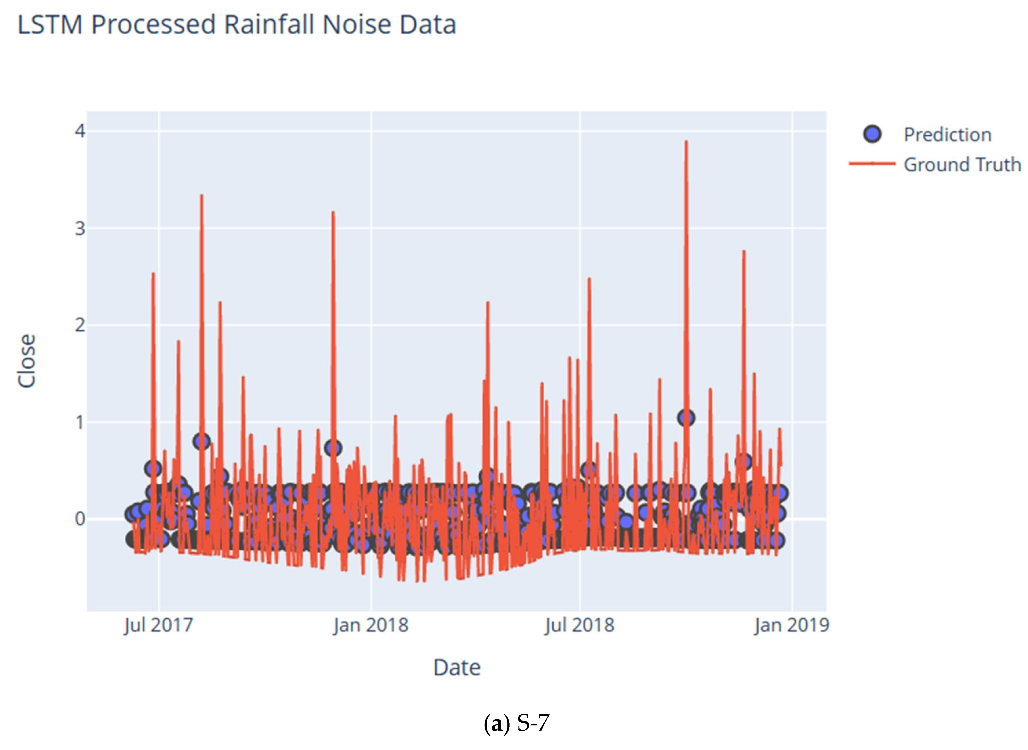
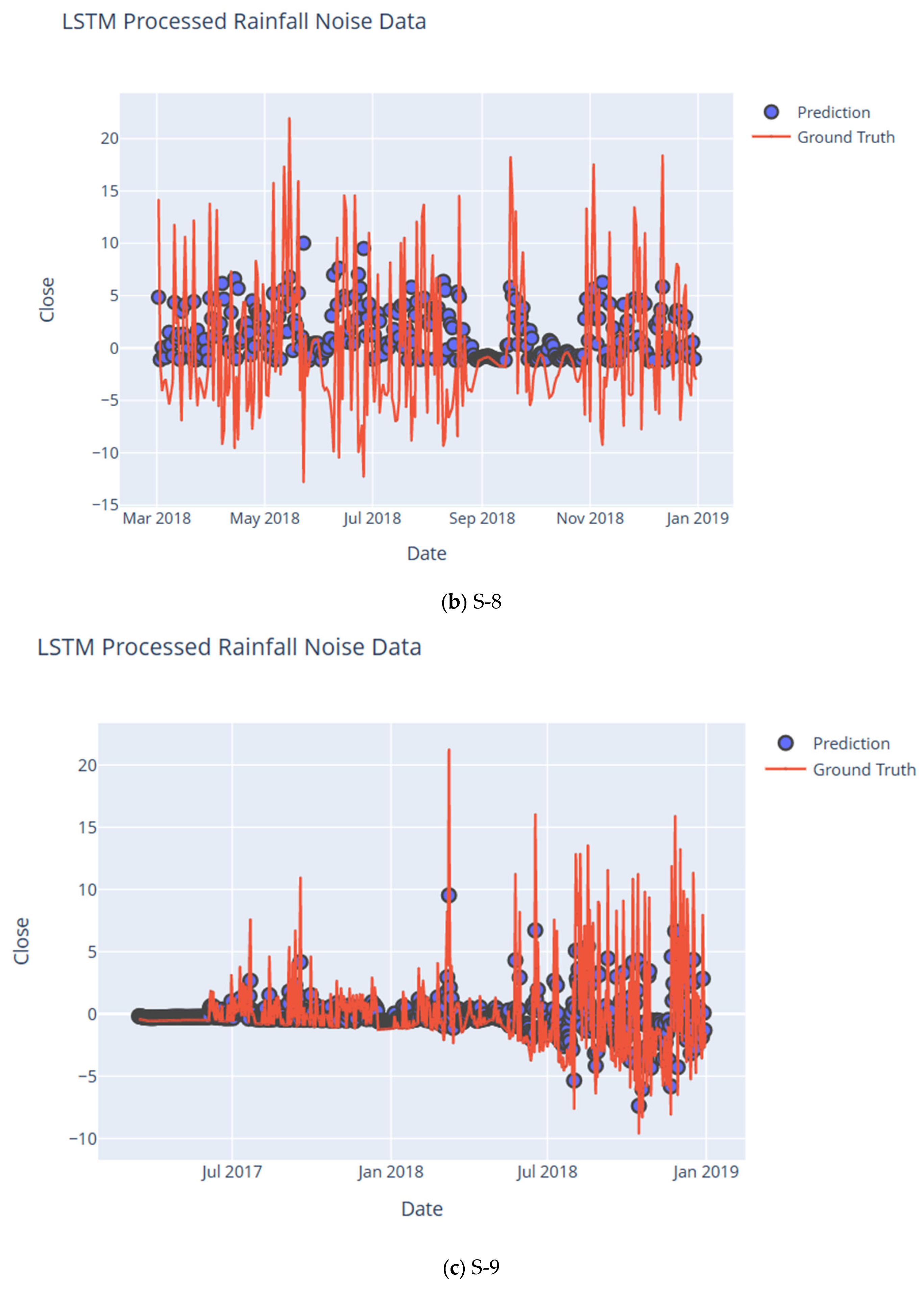
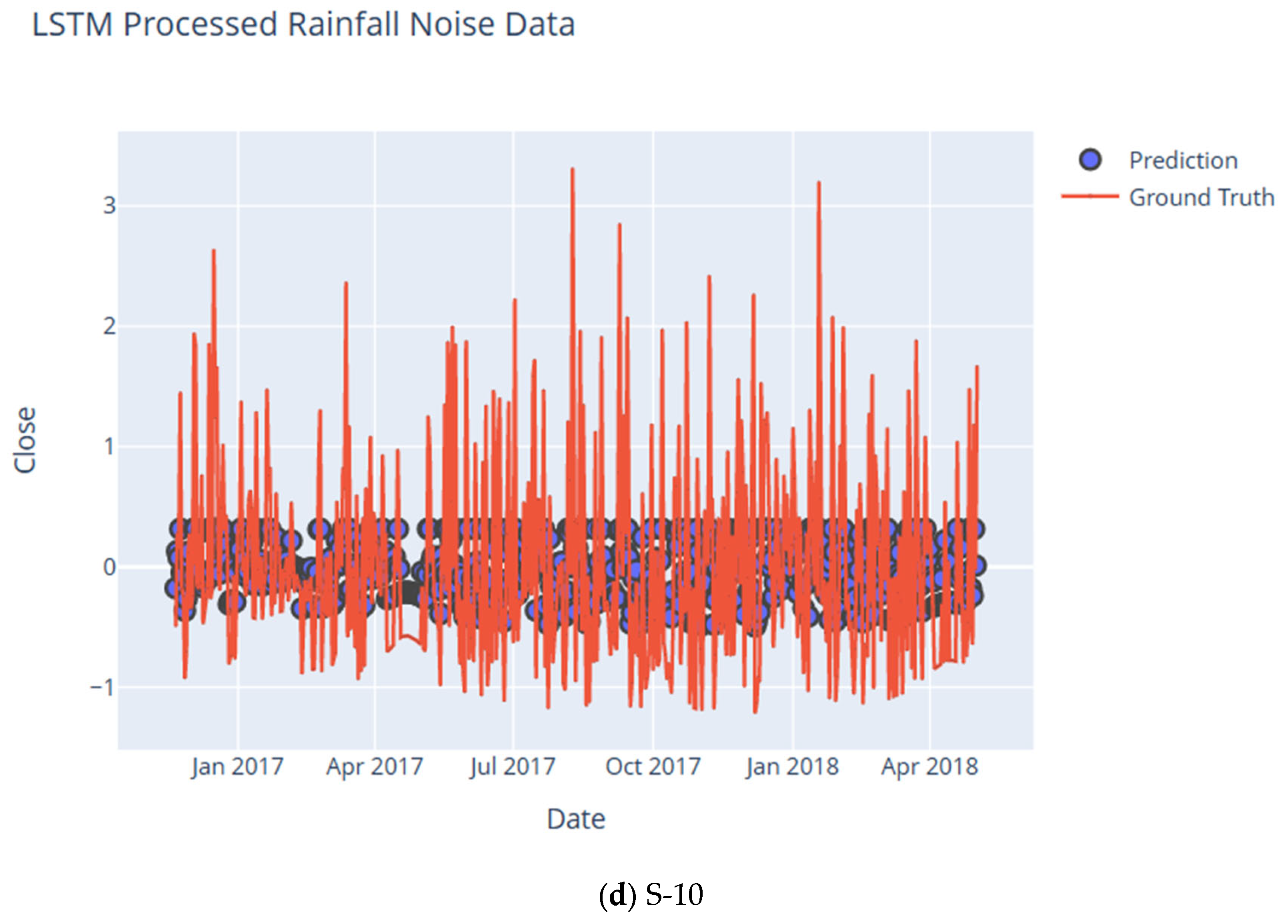
8. Noise Analysis Using DWT and LSTM
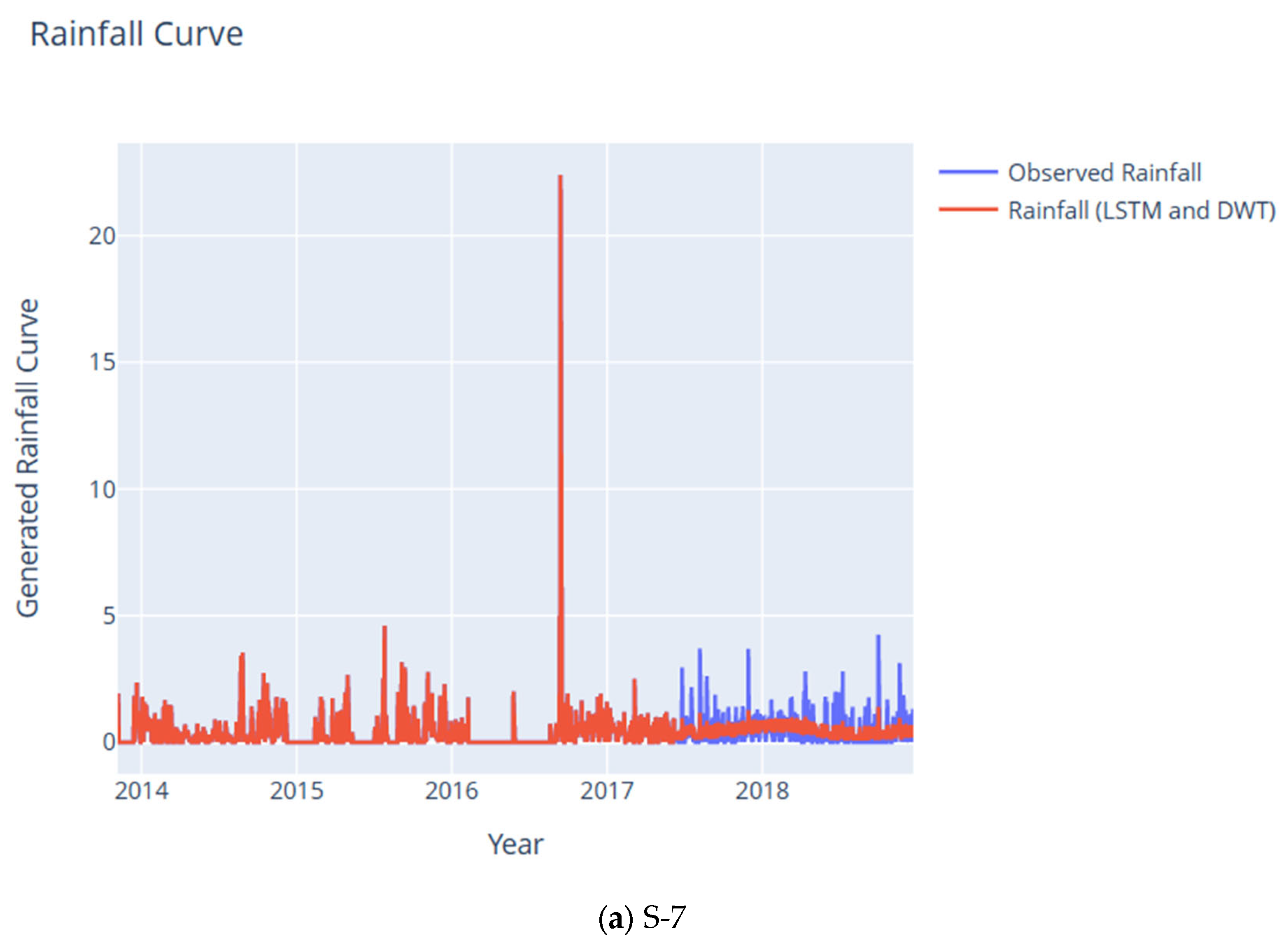
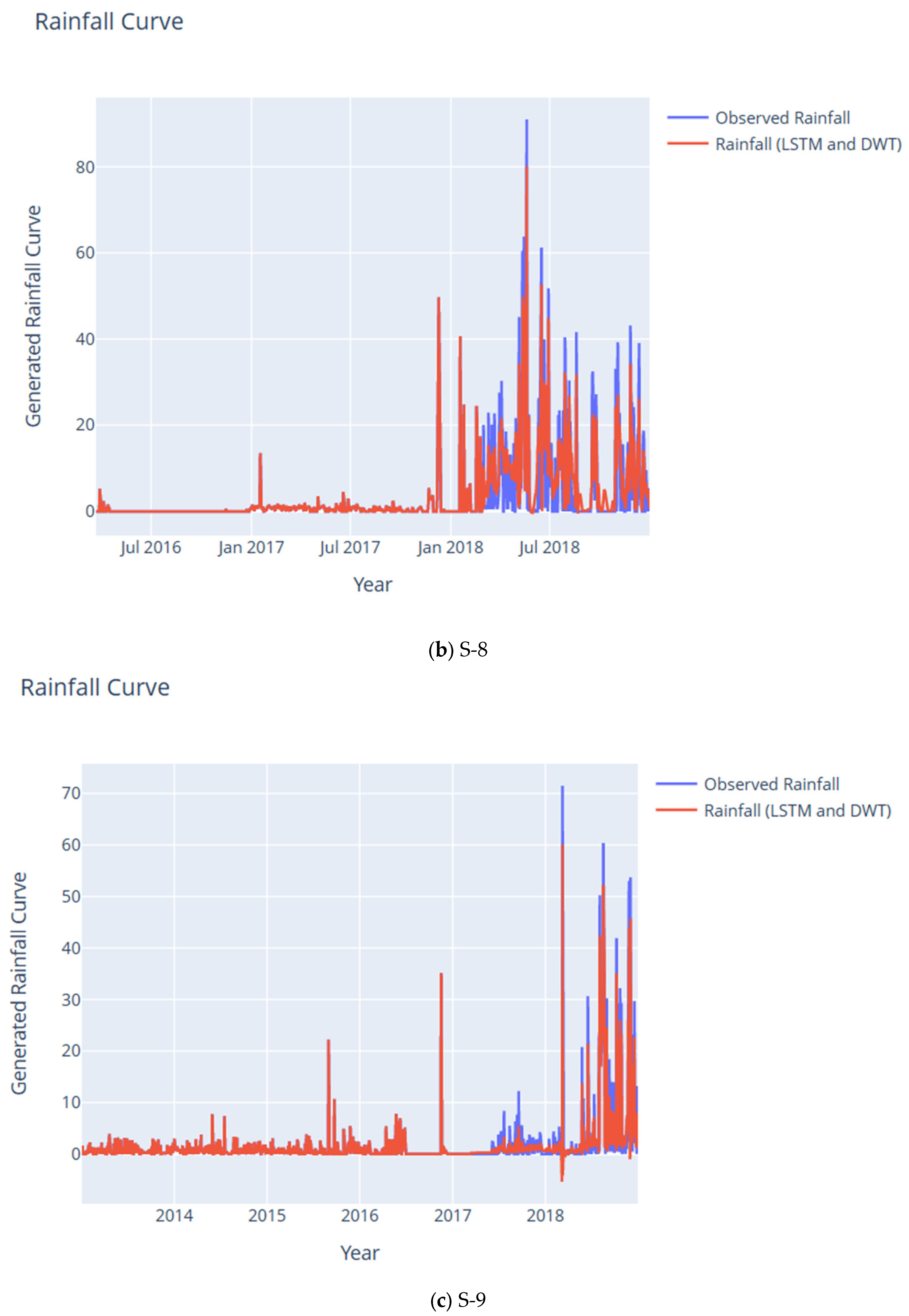
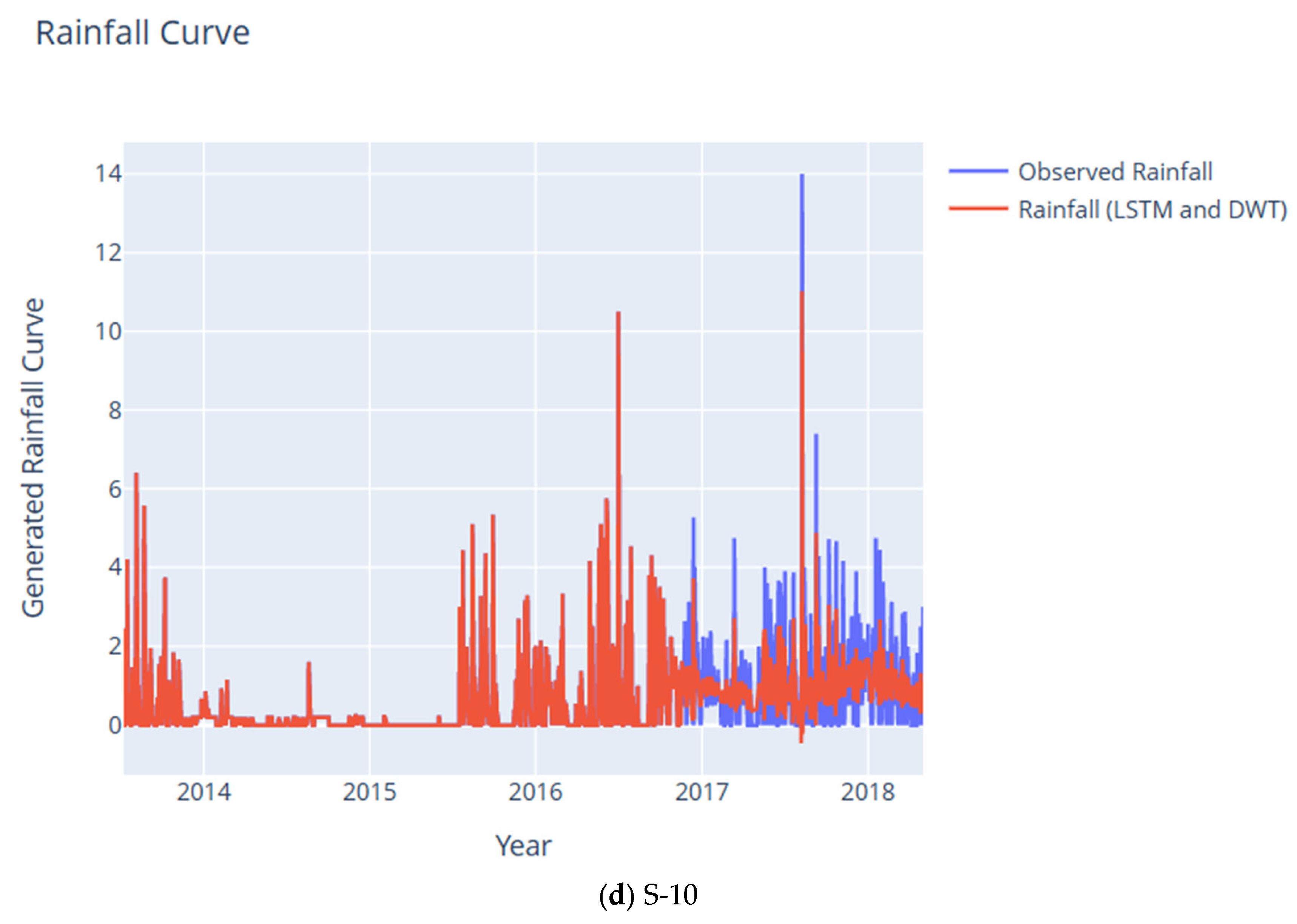
9. Rainfall Noise Modeling Using LSTM
10. Discussion
11. Conclusions
Supplementary Materials
Author Contributions
Funding
Data Availability Statement
Conflicts of Interest
References
- Nalley, D.; Adamowski, J.; Biswas, A.; Gharabaghi, B.; Hu, W. A multiscale and multivariate analysis of precipitation and streamflow variability in relation to ENSO, NAO and PDO. J. Hydrol. 2019, 574, 288–307. [Google Scholar] [CrossRef]
- Gao, L.; Deng, Y.; Yan, X.; Li, Q.; Zhang, Y.; Gou, X. The unusual recent streamflow declines in the Bailong River, north-central China, from a multi-century perspective. Quat. Sci. Rev. 2021, 260, 106927. [Google Scholar] [CrossRef]
- Hochreiter, S.; Schmidhuber, J. Long short-term memory. Neural Comput. 1997, 9, 1735–1780. [Google Scholar] [CrossRef] [PubMed]
- Necesito, I.V.; Velasco, J.M.; Kwak, J.W.; Lee, J.H.; Lee, M.J.; Kim, J.S.; Kim, H.S. Combination of Univariate Long-Short Term Memory Network and Wavelet Transform for predicting dengue case density in the National Capital Region, the Philippines. Southeast Asian J. Trop. Med. Public Health 2021, 52, 479–494. [Google Scholar]
- Feng, Q.; Wen, X.; Li, J. Wavelet Analysis-Support Vector Machine Coupled Models for Monthly Rainfall Forecasting in Arid Regions. Water Resour Manag. 2015, 29, 1049–1065. [Google Scholar] [CrossRef]
- Chen, L.; Sun, N.; Zhou, C.; Zhou, J.; Zhou, Y.; Zhang, J.; Zhou, Q. Performance Enhancement Model for Rainfall Forecasting Utilizing Integrated Wavelet-Convolutional Neural Network. Water Resour Manag. 2020, 34, 2371–2387. [Google Scholar] [CrossRef]
- Kratzert, F.; Klotz, D.; Brenner, C.; Schulz, K.; Herrnegger, M. Rainfall–runoff modelling using long short-term memory (LSTM) networks. Hydrol. Earth Syst. Sci. 2018, 22, 6005–6022. [Google Scholar] [CrossRef] [Green Version]
- Kratzert, F.; Klotz, D.; Herrnegger, M.; Sampson, A.K.; Hochreiter, S.; Nearing, G.S. Toward improved predictions in ungauged basins: Exploiting the power of machine learning. Water Resour. Res. 2019, 55, 11344–11354. [Google Scholar] [CrossRef] [Green Version]
- Damavandi, H.G.; Shah, R.; Stampoulis, D.; Wei, Y.; Boscovic, D.; Sabo, J. Accurate prediction of streamflow using long short-term memory network: A case study in the Brazos River Basin in Texas. Int. J. Environ. Sci. Dev. 2019, 10, 294–300. [Google Scholar] [CrossRef] [Green Version]
- Zhang, D.; Lin, J.; Peng, Q.; Wang, D.; Yang, T.; Sorooshian, S.; Liu, X.; Zhuang, J. Modeling and simulating of reservoir operation using the artificial neural network, support vector regression, deep learning algorithm. J. Hydrol. 2018, 565, 720–736. [Google Scholar] [CrossRef] [Green Version]
- Kumar, D.; Singh, A.; Samui, P.; Jha, R.K. Forecasting monthly precipitation using sequential modelling. Hydrol. Sci. J. 2019, 64, 690–700. [Google Scholar] [CrossRef]
- Qin, J.; Liang, J.; Chen, T.; Lei, X.; Kang, A. Simulating and predicting of hydrological time series based on tensorFlow deep learning. Pol. J. Environ. Stud. 2019, 28, 796–802. [Google Scholar] [CrossRef] [PubMed]
- Yang, S.; Yang, D.; Chen, J.; Zhao, B. Real-time reservoir operation using recurrent neural networks and inflow forecast from a distributed hydrological model. J. Hydrol. 2019, 579, 124229. [Google Scholar] [CrossRef]
- Wan, X.; Yang, Q.; Jiang, P.; Zhong, P.A. A hybrid model for real-time probabilistic flood forecasting using elman neural network with heterogeneity of error distributions. Water Resour. Manag. 2019, 33, 4027–4050. [Google Scholar] [CrossRef]
- Ding, Y.; Zhu, Y.; Feng, J.; Zhang, P.; Cheng, Z. Interpretable spatio-temporal attention LSTM model for flood forecasting. Neurocomputing 2020, 403, 348–359. [Google Scholar] [CrossRef]
- Song, T.; Ding, W.; Wu, J.; Liu, H.; Zhou, H.; Chu, J. Flash Flood Forecasting Based on Long Short-Term Memory Networks. Water 2019, 12, 109. [Google Scholar] [CrossRef] [Green Version]
- He, X.; Luo, J.; Zuo, G.; Xie, J. Daily runoff forecasting using a hybrid model based on variational mode decomposition and deep neural networks. Water Resour. Manag. 2019, 33, 1571–1590. [Google Scholar] [CrossRef]
- Goswami, P.; Srividya. A novel neural network design for long range prediction of rainfall pattern. Curr. Sci. 1996, 70, 447–457. [Google Scholar]
- Chattopadhyay, S. Anticipation of summer monsoon rainfall over India by Artificial Neural Network with Conjugate Gradient Descent Learning. arXiv 2006, arXiv:nlin/0611010. [Google Scholar]
- Kannan, M.; Prabhakaran, S.; Ramachandran, P. Rainfall Forecasting Using Data Mining Technique. Int. J. Eng. Technol. 2010, 2, 397–401. [Google Scholar]
- Chattopadhyay, S.; Chattopadhyay, G. Univariate modelling of summer-monsoon rainfall time series: Comparison between ARIMA and ARNN. C. R. Geosci. 2010, 342, 100–107. [Google Scholar] [CrossRef]
- Kannan, S.; Ghosh, S. Prediction of daily rainfall state in a river basin using statistical downscaling from GCM output. Stoch. Environ. Res. Risk Assess. 2011, 25, 457–474. [Google Scholar] [CrossRef]
- Venkata Ramana, R.; Krishna, B.; Kumar, S.R.; Pandey, N.G. Monthly Rainfall Prediction Using Wavelet Neural Network Analysis. Water Resour. Manag. 2013, 27, 3697–3711. [Google Scholar] [CrossRef] [Green Version]
- Joseph, J.; Ratheesh, T.K. Rainfall Prediction using Data Mining Techniques. Int. J. Comput. Appl. 2013, 83, 11–15. [Google Scholar] [CrossRef]
- Nikam, V.B.; Meshram, B.B. Modeling Rainfall Prediction Using Data Mining Method: A Bayesian Approach. In Proceedings of the 2013 Fifth International Conference on Computational Intelligence, Modelling and Simulation, Washington, DC, USA, 24–25 September 2013; pp. 132–136. [Google Scholar] [CrossRef]
- Prasad, N.; Kumar, P.; Mm, N. An Approach to Prediction of Precipitation Using Gini Index in SLIQ Decision Tree. In Proceedings of the 4th International Conference on Intelligent Systems, Modelling and Simulation, Bangkok, Thailand, 29–31 January 2013; pp. 56–60. [Google Scholar] [CrossRef]
- Dutta, P.S.; Tahbilder, H. Prediction of Rainfall using Data-mining Technique over Assam. Indian J. Comput. Sci. Eng. 2014, 5, 85–90. [Google Scholar]
- Gupta, D.; Ghose, U. A comparative study of classification algorithms for forecasting rainfall. In Proceedings of the 4th International Conference on Reliability, Infocom Technologies and Optimization (ICRITO) (Trends and Future Directions), Noida, India, 2–4 September 2015; pp. 1–6. [Google Scholar] [CrossRef]
- Papacharalampous, G.; Tyralis, H.; Koutsoyiannis, D. Univariate Time Series Forecasting of Temperature and Precipitation with a Focus on Machine Learning Algorithms: A Multiple-Case Study from Greece. Water Resour. Manag. 2018, 32, 5207–5239. [Google Scholar] [CrossRef]
- Phan, T.-T.-H.; Caillault, E.P.; Bigand, A. Comparative Study on Univariate Forecasting Methods for Meteorological Time Series. In Proceedings of the 2018 26th European Signal Processing Conference (EUSIPCO), Rome, Italy, 3–7 September 2018; pp. 2380–2384. [Google Scholar] [CrossRef]
- Tran Anh, D.; Duc Dang, T.; Pham Van, S. Improved Rainfall Prediction Using Combined Pre-Processing Methods and Feed-Forward Neural Networks. J 2019, 2, 65–83. [Google Scholar] [CrossRef] [Green Version]
- Choi, C.; Kim, J.; Kim, J.; Kim, H.S. Development of Combined Heavy Rain Damage Prediction Models with Machine Learning. Water 2019, 11, 2516. [Google Scholar] [CrossRef] [Green Version]
- Wu, X.; Zhou, J.; Yu, H.; Liu, D.; Xie, K.; Chen, Y.; Hu, J.; Sun, H.; Xing, F. The Development of a Hybrid Wavelet-ARIMA-LSTM Model for Precipitation Amounts and Drought Analysis. Atmosphere 2021, 12, 74. [Google Scholar] [CrossRef]
- Wei, M.; You, X. Monthly rainfall forecasting by a hybrid neural network of discrete wavelet transformation and deep learning. Water Resour Manag. 2022, 36, 4003–4018. [Google Scholar] [CrossRef]
- Kabbilawsh, P.; Kumar, D.S.; Chithra, N.R. Performance evaluation of univariate time-series techniques for forecasting monthly rainfall data. J. Water Clim. Change 2022, 13, 4151–4176. [Google Scholar] [CrossRef]
- Tsui, F. Time Series Prediction Using a Multi-Resolution Dynamic Predictor. Ph.D. Thesis, University of Pittsburgh, Pittsburgh, PA, USA, 1996. ISBN 978-0-591-37804-7. [Google Scholar]
- Hsia, C.H.; Chiang, J.S.; Guo, J.M. Multiple Moving Objects Detection and Tracking Using Discrete Wavelet Transform, Discrete Wavelet Transforms. 2011. Available online: https://www.intechopen.com/books/iscrete-wavelet-transforms-biomedical-applications/multiple-moving-objects-detection-and-tracking-using-discrete-wavelet-transform (accessed on 20 June 2020). [CrossRef]
- Patil, G.M.; Rao, K.S.; Satyanarayana, K. Heart disease classification using discrete wavelet transform coefficients of isolated beats. In Proceedings of the 13th International Conference on Biomedical Engineering, Singapore, 3–6 December 2008; Lim, C.T., Goh, J.C.H., Eds.; Springer: Berlin, Germany, 2009. [Google Scholar] [CrossRef]
- Shmueli, G. Wavelet-based monitoring for biosurveillance. Axioms 2013, 2, 345–370. [Google Scholar] [CrossRef] [Green Version]
- Alimohamadi, Y.; Zahraei, S.M.; Karami, M.; Yaseri, M.; Lotfizad, M.; Holakouie-Naieni, K. Aberration detection of pertussis from the Mazandaran province, Iran, from 2012 to 2018: Application of discrete wavelet transform. J. Acute Dis. 2020, 9, 114–120. [Google Scholar] [CrossRef]
- Yim, S.Y.; Wang, B.; Xing, W. Prediction of early summer rainfall over South China by a physical-empirical model. Clim. Dyn. 2014, 43, 1883–1891. [Google Scholar] [CrossRef]
- Goyal, M.K. Monthly rainfall prediction using wavelet regression and neural network: An analysis of 1901–2002 data, Assam, India. Theor. Appl. Climatol. 2014, 118, 25–34. [Google Scholar] [CrossRef]
- Bagirov, A.M.; Mahmood, A.; Barton, A. Prediction of monthly rainfall in Victoria, Australia: Clusterwise linear regression approach. Atmos. Res. 2017, 188, 20–29. [Google Scholar] [CrossRef]
- Abbot, J.; Marohasy, J. Application of artificial neural networks to rainfall forecasting in Queensland, Australia. Adv. Atmos. Sci. 2012, 29, 717–730. [Google Scholar] [CrossRef]
- Abbot, J.; Marohasy, J. Input selection and optimisation for monthly rainfall forecasting in Queensland, Australia, using artificial neural networks. Atmos. Res. 2014, 138, 166–178. [Google Scholar] [CrossRef]
- Hong, K.; Kang, T. A Study on Rainfall Prediction based on Meteorological Time Series. In Proceedings of the 2021 Twelfth International Conference on Ubiquitous and Future Networks (ICUFN), Jeju Island, Republic of Korea, 17–20 August 2021; pp. 302–304. [Google Scholar] [CrossRef]
- Narasimha Murthy, K.V.; Kishore Kumar, G. Distribution and Prediction of Monsoon Rainfall in Homogeneous Regions of India: A Stochastic Approach. Pure Appl. Geophys. 2022, 179, 2577–2590. [Google Scholar] [CrossRef]
- Ray, S.N.; Chattopadhyay, S. Analyzing surface air temperature and rainfall in univariate framework, quantifying uncertainty through Shannon entropy and prediction through artificial neural network. Earth Sci. Inform. 2021, 14, 485–503. [Google Scholar] [CrossRef]
- Chen, B.; Chen, Z.; Wang, G.; Xie, W. Damage Detection on Sudden Stiffness Reduction Based on Discrete Wavelet Transform. Sci. World J. 2014, 2014, 807620. [Google Scholar] [CrossRef] [Green Version]
- Strömbergsson, D.; Marklund, P.; Berglund, K.; Saari, J.; Thomson, A. Mother wavelet selection in the discrete wavelet transform for condition monitoring of wind turbine drivetrain bearings. Wind Energy 2019, 22, 1581–1592. [Google Scholar] [CrossRef]
- Patil, P.B.; Chavan, M.S. A wavelet based method for denoising of biomedical signal. In Proceedings of the International Conference on Pattern Recognition, Informatics and Medical Engineering (PRIME-2012), Salem, India, 21–23 March 2012; pp. 278–283. [Google Scholar] [CrossRef]
- Mathworks. 2012. Available online: https://www.mathworks.com/help/wavelet/gs/choose-a-wavelet.html (accessed on 29 November 2022).
- Jense, A.; la Cour-Harbo, A. Ripples in Mathematics; Springer: Berlin/Heidelberg, Germany, 2001. [Google Scholar]
- Gao, R.X.; Yan, R. Wavelets: Theory and Applications for Manufacturing; Springer: Berlin/Heidelberg, Germany, 2011; ISBN 978-1-4419-1545-0. [Google Scholar]
- Qashqai, P.; Zgheib, R.; Al-Haddad, K. GRU and LSTM Comparison for Black-Box Modeling of Power Electronic Converters. In Proceedings of the IECON 2021—47th Annual Conference of the IEEE Industrial Electronics Society, Toronto, ON, Canada, 13–16 October 2021; pp. 1–5. [Google Scholar] [CrossRef]
- Dolek, I. LSTM. Deep Learning Turkey. 2018. Available online: https://ishakdolek.medium.com/lstm-d2c281b92aac (accessed on 20 June 2020).
- Kingma, D.P.; Ba, J. Adam: A Method for Stochastic Optimization. arXiv 2015, arXiv:1412.6980. [Google Scholar]
- Gupta, H.V.; Kling, H.; Yilmaz, K.K.; Martinez, G.F. Decomposition of the mean squared error and nse performance criteria: Implications for improving hydrological modelling. J. Hydrol. 2009, 377, 80–91. [Google Scholar] [CrossRef] [Green Version]
- Willmott, C.J. On the evaluation of model performance in physicalgeography. In Spatial Statistics and Models; Gaile, G.L., Willmott, C.J., Eds.; D. Reidel: Boston, MA, USA, 1984; pp. 443–460. [Google Scholar] [CrossRef]
- CNN Philippines. Massive Flooding Affects More than 3000 Families in Eastern Samar. 2021. Available online: https://www.cnnphilippines.com/regional/2021/1/12/Eastern-Samar-flooding.html (accessed on 30 August 2022).
- Serafica, R. LOOK: Houses in Eastern Samar town flooded due to Urduja. 2017. Available online: https://www.rappler.com/moveph/191508-houses-taft-eastern-samar-flood-urduja/ (accessed on 30 August 2022).
- PIA (Philippine Information Agency) Eastern Samar. Maslog Mayor Fears Hunger in His Town. 2011. Available online: https://samarnews.com/news_clips16/news317.htm (accessed on 30 August 2022).
- PIA (Philippine Information Agency) Eastern Samar. Philippines: 40,000 Affected, 6 Dead in Floods at Eastern, Northern Samar. 2008. Available online: https://reliefweb.int/report/philippines/philippines-40000-affected-6-dead-floods-eastern-northern-samar (accessed on 30 August 2022).
- Xie, H.; Tang, H.; Liao, Y.-H. Time series prediction based on NARX neural networks: An advanced approach. In Proceedings of the 2009 International Conference on Machine Learning and Cybernetics, Hebei, China, 12–15 July 2009; pp. 1275–1279. [Google Scholar] [CrossRef]
- Koschwitz, D.; Frisch, J.; van Treeck, C. Data-driven heating and cooling load predictions for non-residential buildings based on support vector machine regression and NARX Recurrent Neural Network: A comparative study on district scale. Energy 2018, 165, 134–142. [Google Scholar] [CrossRef]
- Ruslan, F.A.; Samad, A.M.; Zain, Z.M.; Adnan, R. Flood water level modeling and prediction using NARX neural network: Case study at Kelang river. In Proceedings of the 2014 IEEE 10th International Colloquium on Signal Processing and Its Applications, Kuala Lumpur, Malaysia, 7–9 March 2014; pp. 204–207. [Google Scholar] [CrossRef]
- Schoups, G.; Vrugt, J.A. A formal likelihood function for parameter and predictive inference of hydrologic models with correlated, heteroscedastic, and non-Gaussian errors. Water Resour. Res. 2010, 46, 2009WR008933. [Google Scholar] [CrossRef] [Green Version]
- Pryor, S.C.; Schoof, J.T. Changes in the seasonality of precipitation over the contiguous USA. J. Geophys. Res. 2008, 113, D21108. [Google Scholar] [CrossRef]
- Sumner, G.; Homar, V.; Ramis, C. Precipitation seasonality in eastern and southern coastal Spain. Int. J. Climatol. 2001, 21, 219–247. [Google Scholar] [CrossRef]


| Authors | Subject Area | Technique | Variable | Performance Indicator Used |
|---|---|---|---|---|
| [18] | Global | ANN | Mean rainfall | Relative percentage error |
| [19] | Global | ANN | Rainfall | MSE |
| [20] | Global | Regression | Rainfall, humidity, wind direction, minmax temp | MSE |
| [21] | Local | ARIMA, ARNN | Rainfall | IA |
| [22] | Local | Decision Tree, K-mean, Regression tree | Temperature, pressure, wind speed, rainfall | MSE |
| [23] | Local | DWT, ANN | Rainfall | RMSE, R, COE |
| [24] | Local | Clustering, Bayesian regularization | Relative humidity, pressure, temperature, precipitable water, wind speed | Accuracy, precision, recall |
| [25] | Local | Bayesian | Temperature, station level pressure, mean sea level pressure, relative humidity, vapour pressure, wind speed, rainfall | Accuracy |
| [26] | Local | SLIQ decision tree | Humidity, pressure, temperature, wind speed, dew point | Accuracy |
| [27] | Global | Regression | Rainfall | RMSE |
| [28] | Local | Regression tree algorithm, naive Bayes approach, k-nearest neighbour, 5-10-1 pattern recognition neural network | Mean temperature, dew point temperature, humidity, pressure of sea and wind speed | MSE |
| [29] | Local | Neural network, support vector machine | Rainfall | NSE, std. deviation ratio, CC, IA, RMSE |
| [30] | Local | SARIMA, FFNN, Bayesian, time-warping | Rainfall | Similarity, NMAE, RMSE |
| [31] | Local | SD, ANN, DWT | Rainfall | R, RMSE, MAE |
| [32] | Local | Decision tree, random forest, SVM, DNN, linear regression, PCA | Heavy rain damage, rainfall | RMSE, MAPE, CC |
| [33] | Local | ARIMA, DWT, LSTM | Rainfall | RMSE, MAE, R-squared |
| [34] | Local | CNN, LSTM, DWT, DCCNN | Rainfall | RMSE, MAE, NSE |
| [35] | Local | HK-SARIMA, NSTF, YJNSTF, naive | Rainfall | RMSE, MAE, NSE |
| S-7 | S-8 | S-9 | S-10 | |
|---|---|---|---|---|
| count | 1873 | 1015 | 2190 | 1759 |
| mean | 0.37 | 3.18 | 1.44 | 0.58 |
| std | 0.75 | 8.84 | 5.18 | 1.01 |
| min | 0.00 | 0.00 | 0.00 | 0.00 |
| 25% | 0.00 | 0.00 | 0.00 | 0.00 |
| 50% | 0.20 | 0.00 | 0.20 | 0.20 |
| 75% | 0.55 | 1.00 | 0.95 | 0.80 |
| max | 22.40 | 91.00 | 71.50 | 14.00 |
| Subcatchment | RMSE | CC | NSE | KGE | IA | LMI | MAPE | PBIAS | RSR |
|---|---|---|---|---|---|---|---|---|---|
| S-7 | 0.20 | 0.96 | 0.93 | 0.92 | 0.98 | 0.92 | 0.00 | −0.88 | 0.01 |
| S-8 | 2.70 | 0.94 | 0.91 | 0.82 | 0.97 | 0.82 | 0.01 | 10.84 | 0.01 |
| S-9 | 1.28 | 0.98 | 0.94 | 0.87 | 0.98 | 0.87 | 0.00 | 0.22 | 0.01 |
| S-10 | 0.33 | 0.95 | 0.89 | 0.84 | 0.97 | 0.89 | 0.00 | −1.67 | 0.01 |
Disclaimer/Publisher’s Note: The statements, opinions and data contained in all publications are solely those of the individual author(s) and contributor(s) and not of MDPI and/or the editor(s). MDPI and/or the editor(s) disclaim responsibility for any injury to people or property resulting from any ideas, methods, instructions or products referred to in the content. |
© 2023 by the authors. Licensee MDPI, Basel, Switzerland. This article is an open access article distributed under the terms and conditions of the Creative Commons Attribution (CC BY) license (https://creativecommons.org/licenses/by/4.0/).
Share and Cite
Necesito, I.V.; Kim, D.; Bae, Y.H.; Kim, K.; Kim, S.; Kim, H.S. Deep Learning-Based Univariate Prediction of Daily Rainfall: Application to a Flood-Prone, Data-Deficient Country. Atmosphere 2023, 14, 632. https://doi.org/10.3390/atmos14040632
Necesito IV, Kim D, Bae YH, Kim K, Kim S, Kim HS. Deep Learning-Based Univariate Prediction of Daily Rainfall: Application to a Flood-Prone, Data-Deficient Country. Atmosphere. 2023; 14(4):632. https://doi.org/10.3390/atmos14040632
Chicago/Turabian StyleNecesito, Imee V., Donghyun Kim, Young Hye Bae, Kyunghun Kim, Soojun Kim, and Hung Soo Kim. 2023. "Deep Learning-Based Univariate Prediction of Daily Rainfall: Application to a Flood-Prone, Data-Deficient Country" Atmosphere 14, no. 4: 632. https://doi.org/10.3390/atmos14040632