Article

Assessing the Impact of Cumulus Parameterization Schemes on Simulated Summer Wind Speed over Mainland China

1
College of Hydrology and Water Resources, Hohai University, Nanjing 210098, China
2
CMA-HHU Joint Laboratory for Hydrometeorological Studies, Hohai University, Nanjing 210098, China
3
Air Traffic Control and Navigation College, Air Force Engineering University, Xi’an 710000, China
4
Unit No. 75839 of PLA, Guangzhou 510510, China
*
Authors to whom correspondence should be addressed.
Atmosphere 2022, 13(4), 617; https://doi.org/10.3390/atmos13040617
Submission received: 24 February 2022 / Revised: 6 April 2022 / Accepted: 8 April 2022 / Published: 12 April 2022
(This article belongs to the Special Issue Advanced Climate Simulation and Observation)

Abstract

:
Wind speed is an important meteorological parameter, whose simulation is influenced by various physical process parameterizations. However, the impact of cumulus parameterization schemes (CPSs) on wind speed simulation at the climate scale has not been sufficiently investigated in previous studies. Using the Advanced Research version of the Weather Research and Forecasting model (ARWv3) and hydrostatic wind speed change equation, we assessed the effects of four CPSs on a 10 m wind speed simulation over mainland China in the summer of 2003. In general, different CPSs can reproduce the wind speed distribution. Meanwhile, the sensitivity of wind speed simulation to CPSs was found to be the highest in East and southern China, followed by the Tibetan Plateau, and then Northwest China. We found that the main physical processes influencing wind speed (i.e., the pressure gradient (PRE), diffusion (DFN), and convection (CON) terms) vary greatly with sub-regions. CPSs mainly affect the secondary CON that regulates the balance between the dominant terms PRE and DFN, and also has a significant effect on PRE. For example, for CON, the difference index (DIF) between the Kain–Fritsch (KF) and previous KF (pKF) CPSs is larger than 20%, corresponding to a PRE DIF of about 14%. The term of local wind speed change (Vt) is significantly more sensitive to the CPSs than the other terms with a DIF of 283% over the Tibetan Plateau, suggesting high CPS sensitivity of the simulated wind speed. In addition, we explained the causes of the CPS-induced sensitivities. This work helps understand the Weather Research and Forecasting model (WRF) performance and emphasizes the importance of the CPS choice in simulating/forecasting wind speed.

1. Introduction

As one of the key variables of meteorological fields, the simulation and prediction of wind has been a goal of intensive research in various academic and industrial fields [1]. On the one hand, changes in wind direction are important, especially in coastal areas where they affect hydrodynamic factors such as waves and storm surges [2]. On the other hand, the change and distribution of wind speed have a significant influence on the change in the thermal structure of the boundary layer [3], surface fluxes [4], heat transfer, and mass transport [5], and even the estimation of pollutants [6]. Therefore, the studies of the processes affecting wind speed change and the sensitivity of wind speed simulation to different physical schemes are of importance for reference to further understand atmospheric motion. Meanwhile, from the perspective of society and economics, global warming leads to the frequent occurrence of extreme weather (e.g., storms and typhoons), so the forecast of wind speed is also extremely important to reduce economic losses and personal injury [7].
To explore the factors affecting wind speed simulation, it is necessary to understand the effects of atmospheric and land processes on wind speed. Previous studies on wind speed have been mainly based on the direct momentum balance method, i.e., the surface wind vector is determined by pressure gradient force, Coriolis force, gravity, and friction. For example, using this method in a weather case, Van den Broeke and Van Lipzig [8] suggested that large-scale pressure gradient forces controlled the momentum budget on the near-surface and contributed the most to wind speed, while the Coriolis force and gravity wave drag also affected wind speed. Horvath et al. [9] showed through a case study in winter that local and regional thermally driven circulation could influence the air mass through pressure gradient force within the pressure system, which was an important part of wind speed formation. In addition, the effects of land surface properties and their changes on wind speed cannot be ignored. For example, Wen et al. [10] studied the heat circulation of an oasis in the Gobi desert, and their results showed that the changes in land use types and land surface parameters could also change the land surface processes and affect the lower atmosphere and boundary layer with the change in atmospheric circulation situation, humidity, and temperature. Carvalho et al. [1] found that due to the limitation of topographic data for the area with complex terrain, a worse simulation could be produced by the WRF model. Lin et al. [11] studied the wind speed on the Qinghai–Tibet Plateau and pointed out that global warming and cooling caused by atmospheric thermal adaptation would greatly change the surface wind speed at the regional scale, and the surface wind speed on the Qinghai–Tibet Plateau changed more than other regions in mainland China. In addition, Zhang et al. [12] indicated that the pressure gradient force decreased when the wind speed dropped over the Qinghai–Tibet Plateau in summer, mainly due to the adjustment of atmospheric circulation. Zeng et al. [13] derived an equation affecting wind speed change, and the simulation results showed that the Coriolis force had no effect on wind speed, while the main physical processes affecting wind speed change were pressure gradient force, convection and turbulence, and these physical processes showed large differences with regional land perturbations, i.e., the simulation of these processes could be very sensitive to the choice of land surface schemes.
As can be seen from previous simulations of wind speed, there have been many influencing factors involved, among which the relationship between cumulus development and the wind field cannot be ignored. Previous studies of cumulus parameterization schemes (CPSs) were basically related to the study of precipitation, e.g., how cumulus development can affect heavy rainfalls [14], while the influence of CPSs on wind speed simulation has been rarely investigated [13,15]. Srinivas et al. [16] employed a mesoscale model of ARWv3.2, and found that compared to cloud microphysics and boundary layer schemes, the selection of cumulus convection parameterization schemes was more sensitive to tropical cyclone intensity and path. Therefore, different CPSs had influences on the simulation of surface wind speed to varying degrees. In fact, in addition to calculating cloud water content, CPSs are also intended to consider the effects of unresolved deep and shallow convective clouds, in which one of the main purposes is to calculate vertical fluxes caused by subgrid updrafts and downdrafts, as well as corresponding horizontal motions to compensate the change in vertical velocity, i.e., CPSs directly affect grid-scale wind speeds in the model. For example, Asai [17] found that vertical wind shear tended to inhibit the development of convection in the vertical plane parallel to the wind. Sui and Yanai [18] estimated the influence of cumulus clouds on the rotating part of the large-scale momentum field by using the vorticity balance residual, and found that cumulus clouds could slow down the mean airflow, and in the lower troposphere, such deceleration tended to reduce the vertical wind shear of the environment. The relationship between cumulus clouds and wind fields is more complicated in summer when convection is frequent. Das et al. [19] used different CPSs to simulate the Indian summer monsoon, showing that the simulation of typical characteristics of the Indian summer monsoon was quietly different with different schemes, among which the velocity potential and divergent winds obtained by Kuo-type CPS simulation were weak. Using the obliquely rotated principal component analysis, Rao et al. [20] found that the summer topographic convection in China was controlled not only by topographic thermal conditions but also by the dynamic force of increasing wind speed in the mountainous area of the northeast Pearl River Delta. However, these studies have seldom focused on CPS-induced effects on simulated wind speed on the climate scales.
Therefore, the objective of this work is to assess the impact of CPSs on simulated wind speed over mainland China on a seasonal scale. The summer of 2003 was a very special season, during which extreme high temperature and rainstorm events occurred in southern/eastern China [21,22]. In this paper, the sensitivity of simulated summer wind speed to CPSs over typical underlying surfaces of different subregions of China (i.e., Northwest China, NW; East China, EC; and the Tibetan Plateau, TP) was evaluated, with the summer of 2003 taken as the study period. The following section describes the model, designed experiments, data, and relevant methods used in the study. Section 3 presents simulation results, and a summary and discussion are given in Section 4.

2. Methodology and Data

2.1. Model and Experimental Design

This work is a continuation of Zeng et al. [13], who assessed the sensitivity of 10 m wind speed to land surface schemes and the processes affecting wind speed in China during the summer of 2003 using the third version of the Advanced Research WRF (ARWv3) mesoscale model. In the summer of 2003, extremely heavy precipitation [21] and continuous high-temperature weather [22] occurred in eastern China, and there was an overall slightly positive anomaly of 10 m wind speed in mainland China (Figure 1b,c). The model selected in this study is the ARWv3 [23]. The physical schemes used in all experiments were the rapid radiative transfer model (RRTM) for long-wave radiation scheme, Dudhia short-wave radiation scheme, the WRF single moment 5-class microphysics scheme (WSM5), Monin-Obukhov near-surface scheme, Yonsei University (YSU) planetary boundary scheme, and Noah land surface scheme [13].
It should be noted that as a continuation of the work on the impact of land surface schemes (LSSs) on simulated wind speed by Zeng et al. (2018), the present study employs the same model and almost the same suite of model configurations, except for the CPSs, and intends to compare the impact induced by LSSs with that by CPSs. Because Zeng et al. (2018) had used four LSSs, correspondingly, for the sake of comparability, this study uses the four widely-used CPSs as follows: (1) The Kain–Fritsch (new Eta) scheme (KF hereafter; [24]) is an adjustment of the old Kain–Fritsch scheme in the Eta model. Its closure hypothesis is consistent with that of the old KF scheme, and the simple cloud model with water vapor rising and sinking is used to consider the role of entrainments and detrainments with relatively rough microphysical processes. In addition, the scheme inhibits large-scale convections in both marginal unstable and dry environments [25]. (2) The Betts–Miller–Janjic scheme (BMJ hereafter; [26]) is an adjusted and improved Betts–Miller scheme; the thermodynamic profile is relaxed at a given time, and the convective mass flux can consume a certain amount of effective buoyancy. Furthermore, the scheme considers the role of both deep and shallow convection processes. (3) The Grell–Devenyi ensemble scheme (Grell hereafter; [27]) is characterized by a parameterization framework of a simple scheme based on a previous convective parameterization, and this simple scheme was expanded to allow for a series of different assumptions that are commonly used in convective parameterizations with large sensitivity in model simulations, in which values for the assumed parameters are perturbed to obtain the ensemble scheme. (4) The previous Kain–Fritsch (pKF hereafter; [25]) is a one-dimensional entraining/detraining plume model for cumulus clouds, which is characterized by its representation of environmental entrainment and updraft detrainment rates, e.g., the mass exchange between clouds and their environment is regulated at model levels by a buoyancy sorting mechanism.
As in Zeng et al. [13], the simulation domain of in this study is centered at (37° N, 103° E) for mainland China. The total number of grids in the study area is 144 × 116 with horizontal and vertical resolutions of 40 km and 28 levels, and the top pressure of the model is 50 hPa. This area includes three sub-regions (Figure 1a) with typical and contrastive land surface features: NW (arid and semi-arid areas with a large topographic variability), EC (subtropical humid and temperate monsoon climate with high vegetation coverage and flat terrain), and TP (cold climate with high altitudes). The simulation period of all experiments was from 1 May 2003 to 1 September 2003, and the integral time step was 180 s. In order to make the simulation results more robust, here we conducted 12-ensemble experiments, with a small disturbance (i.e., at a 6-h interval) of the starting time of each experiment, i.e., 0000 UTC on 1 May 2003 to 1800 UTC on 3 May 2003 as the initial time of each ensemble. In the consecutive four-month tests, we took the first month as the model spin-up time, and used the simulation results of the ensemble simulation tests in June, July and August to conduct seasonal scale analysis. It should be noted here that we will use the names of CPSs (i.e., KF, BMJ, Grell, and pKF) to represent the ensemble averages of the simulations of the corresponding CPSs. Due to all experiments adopting the same physical parameterization schemes and the same simulation area and time period (i.e., June–August), the differences in simulation results were caused by the differences among the CPSs.

2.2. The Data

The ARW modeling system includes a number of datasets for default options or for users’ selection, e.g., the present study employs a background albedo dataset and a dataset for vegetation indices based on the Moderate Resolution Imaging Spectroradiometer (MODIS) data, and a United States Geological Survey 10 min resolution topography dataset. Following Zeng et al. [13], the FINAL (FNL) 1° × 1° analysis data with a 6 hourly interval provided by the National Centers for Environmental Prediction (NCEP) were used for the initial fields, boundary conditions and validation data for simulation results. The NCEP Climate Forecast System Reanalysis (CFSR) monthly average data with a resolution of 0.5° × 0.5° were used in the anomaly distribution of summer wind speed in 2003 relative to the summer average over the last 30 years (Figure 1b,c).

2.3. Wind Speed Change Equation

Zeng et al. [13] derived the equation for full wind speed (other than wind components), which can be expressed as
V t = ADV + PRE + CON + DFN ,
where the 4 terms ADV, PRE, CON and DFN indicate the influences on local full wind speed change Vt, by advection, pressure gradient force, convection, and turbulent diffusion, respectively, where
ADV = t ( u V x + v V y ) dt ,
PRE = t 1 V ( α u p x + α v p y + u Φ x + v Φ y ) dt ,
CON = σ · V σ dt ,
DFN = t V F V dt ,
where u and v are zonal and meridional wind speed components, respectively. V and V are the wind vector and full wind speed ( V = u 2 + v 2 ), respectively, p is pressure, σ · is the vertical velocity of the coordinate system, α is the specific volume, Φ is the geopotential, and F is the friction. For the above formulas, Vt, ADV, PRE, and CON can be calculated directly through the model outputs, then DFN can be calculated using Equation (1), and therefore the relative contribution of each factor/term to the wind speed change can be investigated.
Compared with the traditional momentum balance equation, the advantage of Equation (1) is that it is a variant of the prognostic equation for full wind speed, and can give exact quantitative results of the physical processes that affect the full wind speed, in which the influence of the Coriolis force on full wind speed is reasonably excluded although it must be considered for wind speed components [13].
By selecting different CPSs, the terms in Equations (1)–(5) can be affected in the following two ways. First, the CPSs can affect the thermodynamic structure of the atmosphere. The CPS-related processes of clouds and precipitation can directly heat the air mass, which changes the air density and also leads to modifications of geostrophic winds and hydrostatic stability in the horizontal and vertical directions, respectively, i.e., the terms of ADV, PRE, and CON, which are, respectively, associated with the wind, temperature (or air density), and stability, can be altered. Furthermore, when precipitation is received at the land surface, the surface energy balance is affected, which also results in a change in hydrostatic stability at the land surface. All of the stability changes would lead to changes in convective activities. Second, the CPSs can affect the dynamic structure of the atmosphere. Affected by cumulus entraining/detraining processes at the subgrid scale, the environmental wind field would be changed for compensation, which further causes the grid-cell averaged change of wind at different heights and can further result in wind shear-related turbulence, i.e., DFN can be altered.

2.4. Measures for Assessment

In order to quantitatively compare the consistency between simulation results and NCEP analysis data and investigate the differences among the CPSs, following Zeng et al. [13], several measures were used for the assessment, i.e., the seasonal mean bias of simulations and reference data (BIAS), the standard deviation (STD; STDM and STDO are for simulations and reference data, respectively), the spatial correlation coefficient (CRMO), and the difference index (DIF) of simulated processes affecting the wind speed in different CPSs, which are computed as follows:
BIAS = M ¯ O ¯ ,
STD M = 1 N i = 1 N ( M i M ¯ ) 2 ,
STD O = 1 N i = 1 N O i O ¯ 2 ,
CR MO = i = 1 N ( M i M ¯ ) ( O i O ¯ ) i = 1 N ( M i M ¯ ) 2 i = 1 N ( O i O ¯ ) 2 ,
DIF = T k 1 ¯ T k 2 ¯ 1 k m k = 1 k m T k ¯ × 100 % , k 1 k 2 , k 1 < k m , k 2 < k m ,
where N is the number of grid points involved in the assessment within a region, M and O represent the simulated and observed values of a quantity, respectively, km is the number of the CPSs (4 in this case) for the difference index DIF, T k ¯ is the regional mean value of a term for a certain physical process in Equation (1) from the CPS as labeled by k. DIF indicates the relative differences in the simulations between the different schemes.

3. Simulated Results

Because the same initial and boundary conditions and almost the same physical options were used in this study, in this section we focus on the CPS-induced differences of the 10 m full wind speed simulations in terms of the 12-member ensemble summer mean results.

3.1. The 10 m Wind Speed

3.1.1. Spatial Distributions

Figure 2 presents the spatial distributions of the seasonal average 10 m surface wind speed simulated by different CPSs. It can be found that except for southeastern mainland China, the CPSs generally well produced the wind speed distributions over almost the entire study domain as compared with the reference FNL data (e.g., Figure 1d vs. Figure 2a). Specifically, with a quite high simulation–reference correlation over the land portion of the study domain (Table 1), the general characteristics of wind speed were successfully simulated by the WRF model, e.g., the low values over the area north of 50° N and over the Indochina peninsula, and high values over North China, Northwest China, the Tibetan Plateau, and the surrounding oceans, showing a larger part of the study domain with simulated wind consistent with the reference data. Relatively, the area with values quite different from/higher than the reference data is small (i.e., over southern China and part of North China).
The wind field distributions by the CPSs appear to be close to each other due to the same initial and boundary conditions, and almost the same physical options as well. Overall, the CPSs tend to moderate the wind speed, i.e., the simulated wind speed is shown to be higher in the reference low wind speed zone and lower in the reference high wind speed zone (Figure 1d, Figure 2a–d). For the three subregions, the simulated wind speeds of the four CPSs decrease from west to east in TP, are larger in the north of NW than in the south, and decrease from southwest to northeast in EC.
However, a closer comparison would lead to clearer and larger differences among the CPSs. It can be seen more clearly from the CPS-induced different fields (Figure 2e–j) that the differences in simulated wind speed between different CPSs are relatively smaller in northern China and larger in southern China. For example, large KF–BMJ differences with absolute values of more than 0.3 m s−1 (Figure 2e) mainly exist in South China, and also a similar amplitude of the BMJ-pKF differences can be observed in the TP, South China, and the EC area around the Shandong Peninsula. This is mainly due to the fact that in the summer, the area of South/East China is a wind convergence region of the East Asian monsoon zone, where prevailing northwesterly wind from Siberia is relatively cold and dry in contrast with the warm and moist southwesterly wind from the Indian Ocean [28]. These two types of contrastive winds converge with approximately the same strength, and therefore fronts are formed which lead to the updrafts in the front zones and favor the release of the convective available potential energy; as a result, a large number of convective activities occur in South/East China. For the TP, the summer climate is controlled by the thermal low, which further brings the biggest portion of convective activities and hence precipitation of the year. All of these suggest that the above areas can be most affected by the CPSs. In addition, the CPS differences can enlarge the differences in simulated wind speed. For example, the pKF scheme is a mass flux parameterization using the Lagrangian parcel method to estimate whether instability exists, whether existing instability can become available for cloud growth, and what the properties of convective clouds could be. In contrast, the KF CPS considers a set of parameterizations including the convective trigger function, the mass flux formulation, and the closure assumptions [24], which makes it very different from pKF in simulating wind speed, e.g., KF presents significantly different wind speed compared with pKF in EC and the TP, with differences as large as about 0.3 m s−1 (Figure 2i). In addition, the Grell CPS makes use of a large variety of assumptions previously introduced in earlier formulations, with the assumptions generating a large spread in the solution for the ensemble scheme [27], which makes the CPS very unique as compared to a single scheme such as the other CPSs in the present study. As a result, the Grell–BMJ difference is apparently large in southern China (Figure 2f).
Correspondingly, the Student’s t-test results at the 0.10 significance level [29] show that there is a quite large total area with significant differences, mostly in the southeast of mainland China. This further confirms that wind speed simulation is sensitive to the CPSs in areas with high convective precipitation. At the same time, there are some differences in the results of these CPS-produced simulations, e.g., the BMJ-pKF, KF-pKF and Grell-pKF differences are mainly distributed in the southeast of mainland China, while the total area with significant differences between KF and Grell is small, which is consistent with the above-mentioned results.

3.1.2. Assessment Results

Figure 3a shows the BIAS of the average seasonal wind speed simulated by different CPSs in the total area and each subregion. It can be seen that the wind speed values of the total area and subregions simulated by the four CPSs are similar to those of different land surface schemes [13]. For example, for simulated wind speeds of the total area, NW and EC are higher than the reference, while the TP value is lower. This result is closely associated with the distributions of simulated surface air temperatures. Generally, the model produced higher surface air temperatures over different parts of mainland China except for the TP (not shown). This means that the CPSs produced low-level stratifications that were more stable than they should have been over the TP, which does not favor the downward momentum transport and results in a lower wind speed in the TP. Similarly, simulated wind speed for subregions other than the TP is higher.
In terms of BIAS, the CPSs present an overall higher wind speed for the total area (with the BIASs less than 0.50 m s−1) while sub-regions might show different results, e.g., the BIAS of East China is much larger, and there exists a negative BIAS in the TP. In addition, wind speed in NW (EC) is the best (worst) simulated among the sub-regions, which is consistent with the above-mentioned results of wind speed distributions, e.g., there are much higher wind speed values in EC compared with the reference data (Figure 2 vs. Figure 1d).
The sensitivities of simulated wind speed to CPSs vary in different sub-regions. For example, although CPS-induced BIAS differences are relatively small for EC, while for NW, TP, and the total area, the differences can be much larger between the least and the largest, e.g., compared with the Grell BIAS of about −0.40 m s−1, the amplitude of the pKF BIAS is approximately 50% larger for the TP, and for the total area, the BIAS differences also show the largest amplitude change of 70% as compared to the pKF BIAS of 0.30 m s−1 with the BMJ BIAS of 0.50 m s−1.
Figure 3b shows the CPS-induced difference between STDM and STDO for the seasonal wind speed in the total area and sub-regions. Obviously, among the study sub-regions, the difference amplitude of the four schemes in EC is the smallest (less than 0.05 m s−1), while the difference amplitude in NW is the largest (around −0.4 m s−1), showing that although for different sub-regions simulated spatial variability is quite different with small CPS-induced changes, the CPS-induced changes for the total area are very large, e.g., the STDM -STDO difference amplitude by BMJ is 60% larger than that by KF.
It is noteworthy that in Figure 3b, the fluctuations of wind speeds are all smaller than the reference data. Possible reasons for this result are as follows. (1) Some influences of land surface heterogeneity are probably missing from the simulation. The subgrid heterogeneity could induce modifications of grid-scale changes in surface variables such as wind speed. For example, microscopic topography could dynamically change the atmospheric flow [30], subgrid variations in the surface moisture could thermally induce mesoscale circulations [31], and all of these could lead to grid-scale changes [32]. (2) The model has some deficiencies in simulating the wind speed, e.g., the simulated temperature fields were not well simulated, which would affect vertical momentum transport and then wind speed (as stated above). (3) Models are generally difficult to reproduce extremes of observations, suggesting that they tend to give moderate results compared to observations.
In addition, Table 1 lists the correlation (CRMO) values by the CPSs for the sub-regions. Overall, the CPSs present wind speed patterns quite consistent with the reference (i.e., the CRMO values are approximately 0.7). However, the values differ from sub-regions greatly, and moreover, large CPS-induced CRMO difference can be seen, e.g., the KF–Grell difference amounts to up to 0.14 for the TP.
In general, the assessment measures show that the simulated wind speed is sensitive to the CPSs with different sub-regional characteristics, suggesting that the CPS choice or improvement is important for seasonal wind speed simulations or forecasts. Meanwhile, it is worth noting that the CPS-induced sensitivity is less than that induced by land surface schemes [13].

3.2. Processes Affecting Wind Speed Change

According to the summer mean integral results of Vt, ADV, PRE, CON, and DFN (Table 2), the main processes affecting the wind speed changes are PRE, DFN, and CON, and the effects of PRE and DFN are much larger than that of CON, having a positive and a negative contribution to wind speed, respectively, which is consistent with Zeng et al. [13]. Meanwhile, due to the influence of climate characteristics, there are certain differences in the factors affecting wind speed variation in different subregions. For subregion NW, PRE and DFN of KF have the greatest impacts among those of the CPSs, with both mean integral values of five and four times as large as that of CON, respectively, while PRE and DFN of the other schemes are also 3–5 times higher than CON. For EC, the absolute values of the mean integral PRE and DFN are the largest by BMJ, which are about three and four times larger than that of CON, respectively, but the signs of PRE and DFN are opposite (i.e., they have opposite effects on wind speed change). For the TP, a striking feature of CON appears: the CON contribution to the wind speed change is negative (i.e., the weak updraft formed by the thermal low pressure in summer restrained downward momentum transfer), which is the opposite of the facts observed for EC and NW. In addition, the integral means of PRE and DFN by Grell are the largest for the TP, reaching 12 and 11 times that of CON, respectively.
As can be seen from the difference index DIF of the terms in Equation (1) simulated by different CPSs (Table 3), the least term Vt is much more sensitive to CPSs than the other terms. Among them, the Vt DIF values in NW are less than 40%, while the DIF by pKF and Grell in EC and TP can reach 283% and 106%, respectively. Except Vt, the sensitivities of the other terms to CPSs are complicated. For example, CON is most sensitive to CPSs in NW, with a maximum DIF of 24%, while DFN is the least sensitive. For EC, the sensitivity of each term to CPSs is the lowest among the three sub-regions, with absolute DIF values within 13%. For the TP, CON has the largest effect (corresponding to a maximum DIF amplitude of −95%), followed by ADV, while the DIF maxima of PRE and DFN are lower than 12%. Compared with the sub-regions of EC and NW that show moderate CPS-induced sensitivities in the three major terms (i.e., PRE, DFN, and CON), the TP displays an apparently higher sensitivity, e.g., the DIF between KF and pKF can reach 95% for CON, suggesting that the influence of CPSs on wind speed processes varies greatly with sub-regions. For the overall wind speed change, it suggests that the CPS-induced influence on Vt is great in EC, probably due to frequent convective activities in the summer monsoon; for an even higher CPS-induced influence on Vt in the TP, the high topographic elevations that lead to a thin troposphere in this area could be a main cause.

3.3. Associated Boundary-Layer Parameters

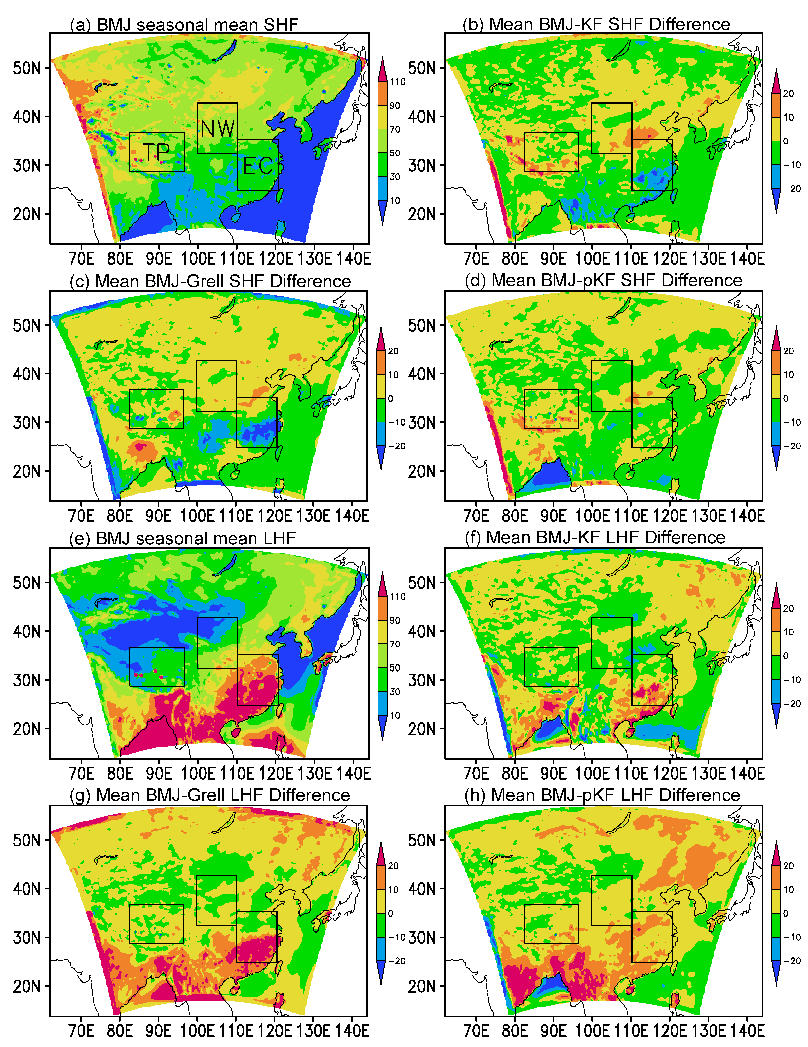
3.3.1. Near-Surface Fluxes

The change in convective activities can affect the change in surface energy fluxes, while the change in surface sensible and latent heat fluxes will affect the convective processes and wind speed through energy transfer and release in the vertical direction with land surface disturbances. Figure 4 shows the average sensible and latent heat fluxes simulated by different CPSs. It can be seen that although CPS-induced sensible and latent heat flux differences are relatively small over most of mainland China, the largest differences still exist in EC (e.g., with an amplitude of over 20 w m−2; Figure 4c,g), which is consistent with the above-mentioned result that over this area, simulated convective activities are affected by the CPSs to quite an extent.
By comparing the difference field of wind speed with that of sensible/latent heat flux, there appears no clear correlation. This suggests that the CPS-induced sensitivities are complicated. Although the land surface plays an important role in modifying 10 m wind speed [13], the changes in surface fluxes are probably less important in CPS-induced changes in wind speed compared with the changes in the interior atmosphere.

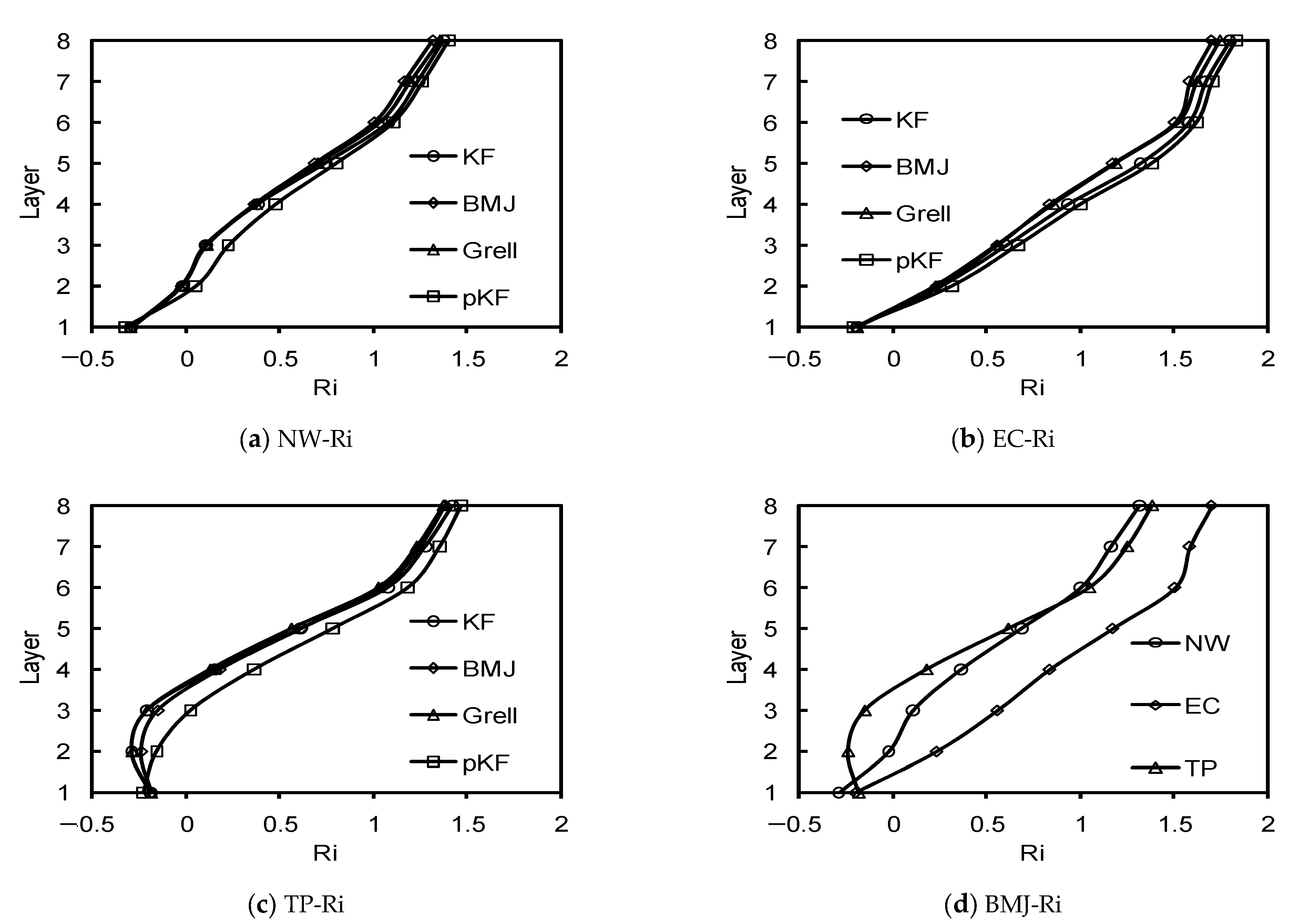
3.3.2. Atmospheric Boundary Layer Stability

On the weather scale, different CPSs can influence simulated momentum exchange by influencing the stability of the simulated atmospheric boundary layer, i.e., the stability of the atmospheric boundary layer can be affected by the energy release in the convective process, which will lead to a difference in the momentum exchange between the upper and lower levels and thus affect the wind speed [1]. Figure 5 shows the CPS-produced seasonally average Richardson number (Ri), which can be used as a measure for atmospheric boundary layer stability. On the whole, similar to the simulation by different land surface schemes that presented the vertical distributions of atmospheric stability in the three sub-regions [13], it can be also concluded that the CPS-produced instability layer over the TP is the thickest, followed by NW and EC (e.g., Figure 5d). Consistent with the above-mentioned results for the sub-regions, the Ri for NW is not sensitive to the CPSs, while the TP shows the highest sensitivity, e.g., there is a quite large Ri difference between Grell and pKF (Figure 5c), corresponding to the highest sensitivity of CON to the CPSs, as addressed in Section 3.2. In addition, Grell produces a more unstable boundary layer than pKF does, which favors the downward momentum transfer, further strengthens the 10 m wind speed, and results in a higher Grell wind speed compared to pKF (Figure 2j). Note that the simulated wind speed sensitivity for the TP is not the highest of the CPSs., i.e., the DIF of Vt for the TP is not the largest among the sub-regions (Table 3). The reason for this complexity is that vertical momentum transfer is a result of convection (i.e., CON), while there are other important processes responsible for wind speed change (e.g., PRE).

4. Summary and Discussion

In order to investigate the sensitivity of simulated wind speed and its influencing processes to the CPS choice, we selected four CPSs (KF, BMJ, Grell, and pKF) as employed in the mesoscale model WRFv3 to separately conduct ensemble simulations for the summer of 2003 in mainland China. Using the wind speed change equation under the hydrostatic condition, we calculated the four physical terms responsible for the wind speed change (Vt), i.e., the terms induced by advection (ADV), pressure gradient force (PRE), convection (CON), and turbulent diffusion (DFN), and quantified the relative importance of influencing processes and analyzed their sensitivities to the CPSs. The main results and conclusions are as follows:
(1)
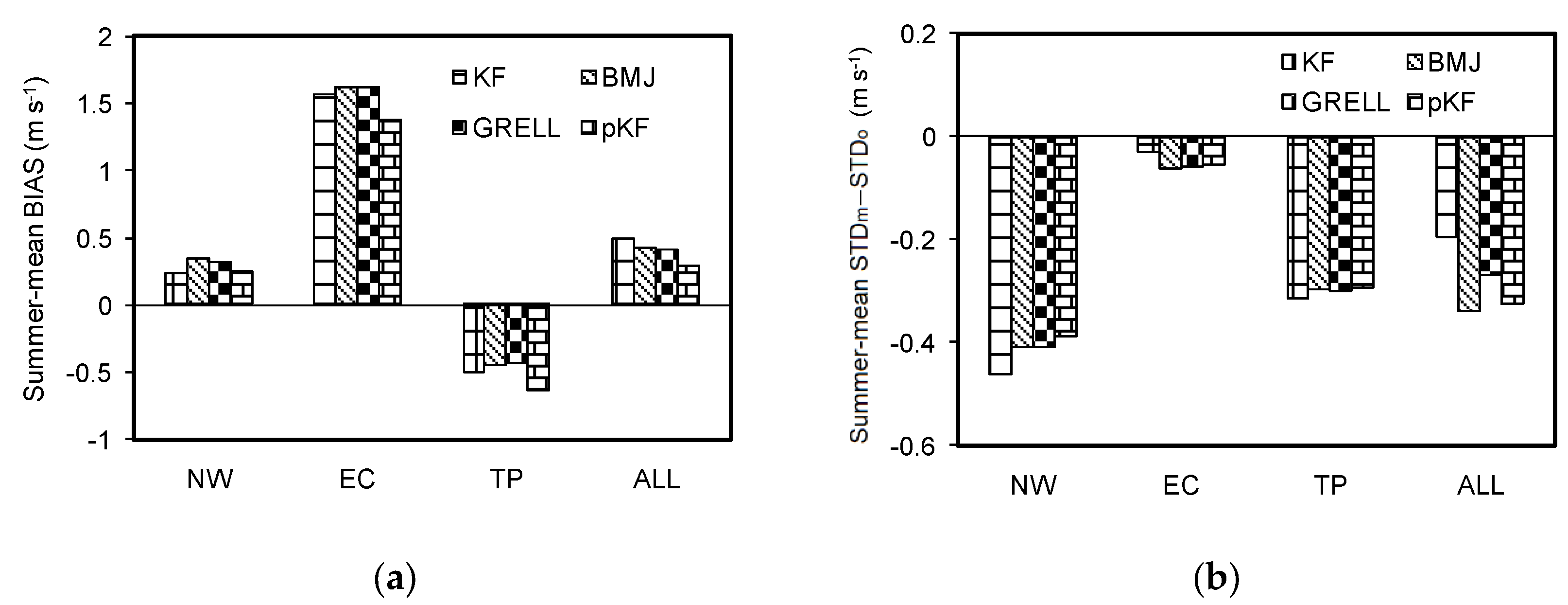
By and large, different CPSs can reproduce 10 m wind speed over mainland China, which is also indicated by the simulation–reference correlation efficiency of approximately 0.70. Previous studies of CPSs were basically associated with precipitation [14], while this result indicates an overall performance of simulating wind speed by the CPSs.
(2)
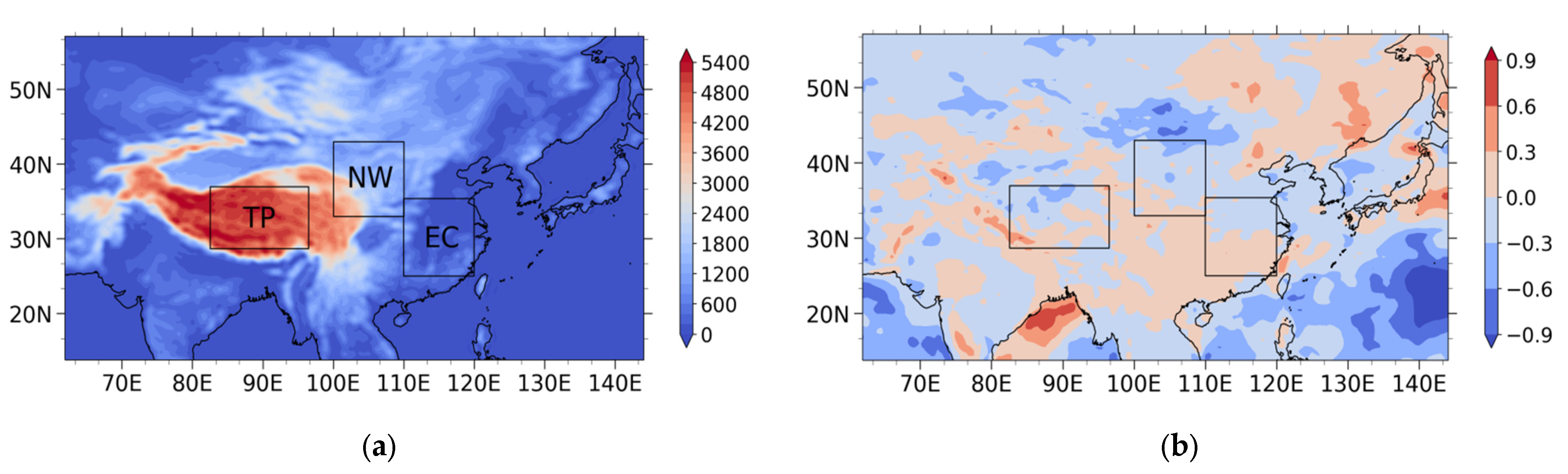
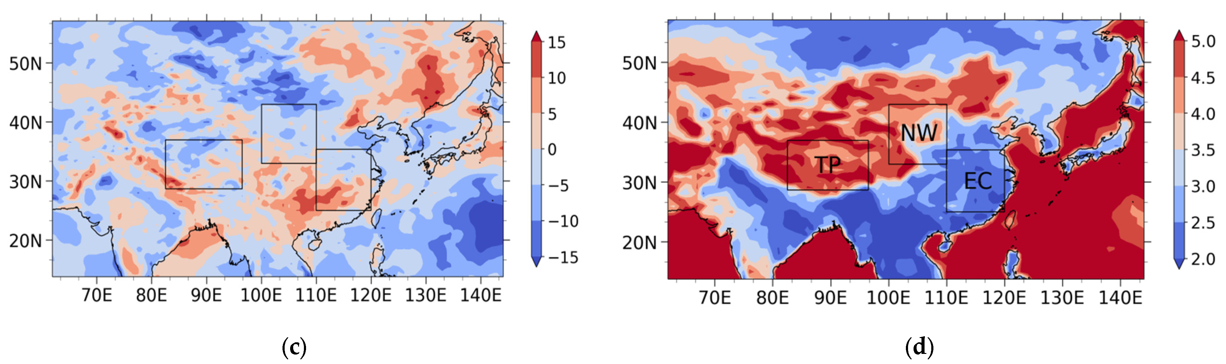
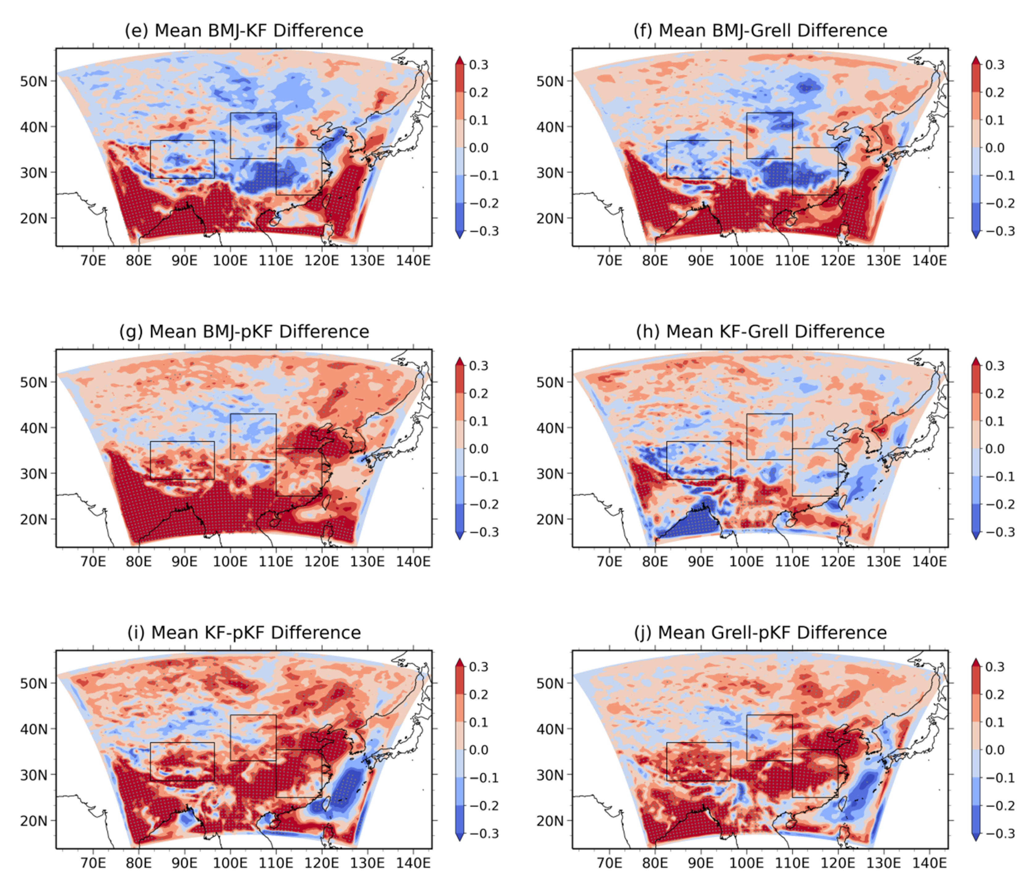
In comparison to the CPS ensembles, the largest simulated difference is generally found between Grell and pKF. Although the CPS choice does not greatly modify the simulated wind speed, sub-regions of mainland China show quite a large CPS-induced impact on wind speed. It can be seen that northern China is relatively unaffected by the CPSs, but southern China, East China, and the Tibetan Plateau are affected to quite large extents, as is confirmed by Student’s t-tests. These high sensitivities are associated with the frequent convective activities in the summer monsoon (e.g., over East China) and a relatively thin troposphere (i.e., over the Tibetan Plateau). Because the influence of CPSs on wind speed simulation has been rarely investigated on a climate scale [13,15], these results clearly indicate where the simulated wind speed is greatly affected in mainland China on the summer scale, and the mechanisms have been revealed.
(3)
Among the terms of influencing processes, CON is most affected by the CPSs, followed by PRE and DFN, corresponding to CPS-induced DIF values of 95%, 14%, and 12% for the sub-regions, respectively. ADV is a secondary term for contribution to Vt, with the latter having a large DIF value of 283% for East China. Previous works seldom showed the CPS-induced impacts on complete influencing processes [14]; this study presents the impacts of the turbulence effect (DFN) and revealed that they cannot be conventionally quantified.
(4)
The results of the related boundary layer parameters can demonstrate the CPS-induced impact on simulated wind speed, in which surface fluxes do not show clear correlations with wind change while the Richardson number does. This suggests that compared with the CPS-induced changes in wind speed in the interior atmosphere, the CPS-induced changes of surface fluxes are less important. This work makes an incremental advance in wind speed study based on the LSS-induced impact [13], emphasizing the importance of the atmospheric process rather than land surface processes.
Because CPSs are closely associated with precipitation simulations, it is expected that there is a correlation between simulated precipitation and wind speed as induced by the CPSs. We found that simulated precipitation is sensitive to the CPSs over the selected subregions, especially over EC (not shown). However, the precipitation–wind speed correlation is complicated. On the one hand, higher precipitation generally means more frequent convective activities that would strengthen surface wind speed by stronger downward momentum transport. On the other hand, precipitation-related surface cooling would strengthen the low-level stable stratification and then restrain downward momentum transport. All of these are likely to lead to opposite results (not shown), i.e., that no definite correlation between CPS-induced precipitation and wind speed can be validated.
It is noteworthy that this work is a case study focusing on the quantitative assessment of physical processes affecting summer wind speeds and their sensitivities to CPSs with a regional climate model. Due to the complexity of the CPSs, the differences in the physical parametrizations of the specific CPSs have not been discussed here. As addressed in previous studies [1,13], the coupled-model simulation reflects not only the performance of a single scheme that is coupled to the model, but also the overall performance of the modeling system, which suggests that this CPS evaluation is of significance to our understanding of the CPS performance and improving the model to simulate the summer wind speed.

Author Contributions

Conceptualization, X.-M.Z. and Y.-Q.Z.; methodology, S.-J.L., M.W., S.-B.S. and X.Y.; software, M.W.; validation, S.-J.L., S.-B.S. and M.W.; formal analysis, S.-J.L., X.Y. and M.W.; investigation, S.-J.L. and M.W.; resources, S.-J.L. and M.W.; data curation, M.W.; writing—original draft preparation, S.-J.L., X.Y. and X.-M.Z.; supervision, X.-M.Z. and Y.-Q.Z.; project administration, X.-M.Z.; funding acquisition, X.-M.Z. All authors have read and agreed to the published version of the manuscript.

Funding

This research was financially supported by the National Natural Science Foundation of China (Grant Nos. U2240248, 41775087 and 41675007), and the National Key Research and Development Program of China (Grant Nos. 2018YFA0606004 and 2018YFC1508200).

Informed Consent Statement

Not applicable.

Data Availability Statement

The FNL Data Archive is managed by the Data Engineering and Curation Section of the Computational and Information Systems Laboratory at the National Center for Atmospheric Research in Boulder, Colorado. The National Center for Atmospheric Research is sponsored by the National Science Foundation.

Acknowledgments

The authors would like to thank three anonymous reviewers for their comments and suggestions which helped in improving the manuscript.

Conflicts of Interest

The authors declare no conflict of interest.

References

  1. Carvalho, D.; Rocha, A.; Gómez-Gesteira, M.; Santos, C. A sensitivity study of the WRF model in wind simulation for an area of high wind energy. Environ. Model. Softw. 2012, 33, 23–34. [Google Scholar] [CrossRef] [Green Version]
  2. McInnes, K.L.; Erwin, T.A.; Bathols, J.M. Global climate model projected changes in 10 m wind speed and direction due to anthropogenic climate change. Atmos. Sci. Lett. 2011, 12, 325–333. [Google Scholar] [CrossRef]
  3. He, Y.; Monahan, A.H.; McFarlane, N.A. Diurnal variations of land surface wind speed probability distributions under clear-sky and low-cloud conditions. Geophys. Res. Lett. 2013, 40, 3308–3314. [Google Scholar] [CrossRef]
  4. Monahan, A.H. The probability distribution of sea surface wind speeds. Part I: Theory and sea winds observations. J. Clim. 2006, 19, 497–520. [Google Scholar] [CrossRef]
  5. Cakmur, R.; Miller, R.; Torres, O. Incorporating the effect of small-scale circulations upon dust emission in an atmospheric general circulation model. J. Geophys. Res. 2004, 109, D07201. [Google Scholar] [CrossRef] [Green Version]
  6. Hu, X.M.; Klein, P.M.; Xue, M. Evaluation of the updated YSU planetary boundary layer scheme within WRF for wind resource and air quality assessments. J. Geophys. Res. Atmos. 2013, 118, 10490–10505. [Google Scholar] [CrossRef]
  7. Schwierz, C.; Köllner-Heck, P.; Mutter, E.Z.; Bresch, D.N.; Vidale, P.; Wild, M.; Schär, C. Modelling European winter wind storm losses in current and future climate. Clim. Chang. 2010, 101, 485–514. [Google Scholar] [CrossRef] [Green Version]
  8. Van den Broeke, M.R.; van Lipzig, N.P.M. Factors controlling the near-surface wind field in Antarctica. Mon. Weather Rev. 2003, 131, 733–743. [Google Scholar] [CrossRef]
  9. Horvath, K.; Koracin, D.; Vellore, R.; Jiang, J.; Belu, R. Sub-kilometer dynamical downscaling of near-surface winds in complex terrain using WRF and MM5 mesoscale models. J. Geophys. Res. 2012, 117, D11111. [Google Scholar] [CrossRef] [Green Version]
  10. Wen, X.H.; Lu, S.H.; Jin, J.M. Integrating remote sensing data with WRF for improved simulations of oasis effects on local weather processes over an arid region in Northwestern China. J. Hydrometeorol. 2012, 13, 573–587. [Google Scholar] [CrossRef]
  11. Lin, C.G.; Yang, K.; Qin, J.; Fu, R. Observed coherent trends of surface and upper-air wind speed over China since 1960. J. Clim. 2013, 26, 2891–2903. [Google Scholar] [CrossRef] [Green Version]
  12. Zhang, H.L.; Pu, Z.X.; Zhang, X.B. Examination of Errors in Near-Surface Temperature and Wind from WRF Numerical Simulations in Regions of Complex Terrain. Weather Forecast. 2013, 28, 893–914. [Google Scholar] [CrossRef] [Green Version]
  13. Zeng, X.M.; Wang, M.; Wang, N.; Yi, X.; Chen, C.H.; Zhou, Z.G.; Wang, G.L.; Zheng, Y.Q. Assessing simulated summer 10-m wind speed over China: Influencing processes and sensitivities to land surface schemes. Clim. Dyn. 2018, 50, 4189–4209. [Google Scholar] [CrossRef]
  14. Kotroni, V.; Lagouvardos, K. Precipitation forecast skill of different convective parameterization and microphysical schemes: Application for the cold season over Greece. Geophys. Res. Lett. 2001, 28, 1977–1980. [Google Scholar] [CrossRef]
  15. Cohen, C. A comparison of cumulus parameterizations in idealized sea-breeze simulations. Mon. Weather Rev. 2002, 130, 2554–2571. [Google Scholar] [CrossRef]
  16. Srinivas, C.V.; Bhaskar, R.D.V.; Yesubabu, V.; Baskaran, R.; Venkatraman, B. Tropical cyclone predictions over the bay of bengal using the high-resolution advanced research weather research and forecasting (ARW) model. Q. J. R. Meteor. Soc. 2013, 139, 1810–1825. [Google Scholar] [CrossRef]
  17. Asai, T. Cumulus Convection in the Atmosphere with Vertical Wind Shear: Numerical Experiment. J. Meteorol. Soc. Jpn. 1964, 42, 245–259. [Google Scholar] [CrossRef] [Green Version]
  18. Sui, C.H.; Yanai, M. Cumulus Ensemble Effects on the Large-Scale Vorticity and Momentum Fields of GATE. Part I: Observational Evidence. J. Atmos. Sci. 1986, 43, 1618–1642. [Google Scholar]
  19. Das, S.; Mitra, A.K.; Iyengar, G.R.; Mohandas, S. Comprehensive test of different cumulus parameterization schemes for the simulation of the Indian summer monsoon. Arch. Meteorol. Geophys. Bioclimatol. Ser. B 2001, 78, 227–244. [Google Scholar] [CrossRef]
  20. Rao, X.N.; Zhao, K.; Chen, X.C.; Huang, A.N.; Xue, M.; Zhang, Q.H.; Wang, M.J. Influence of Synoptic Pattern and Low-Level Wind Speed on Intensity and Diurnal Variations of Orographic Convection in Summer over Pearl River Delta, South China. J. Geophys. Res. Atmos. 2019, 124, 6157–6179. [Google Scholar] [CrossRef]
  21. Zeng, X.M.; Wu, Z.H.; Song, S.; Xiong, S.Y.; Zheng, Y.Q.; Zhou, Z.G.; Liu, H.Q. Effects of land surface schemes on the simulation of a heavy rainfall event by WRF. Chin. J. Geophys. 2012, 55, 16–28. [Google Scholar] [CrossRef]
  22. Zeng, X.M.; Wang, B.; Zhang, Y.; Zheng, Y.; Wang, N.; Wang, M.; Yi, X.; Chen, C.; Zhou, Z.; Liu, H. Effects of land surface schemes on WRF-simulated geopotential heights over China in summer 2003. J. Hydrometeorol. 2016, 17, 829–851. [Google Scholar] [CrossRef]
  23. Skamarock, W.C.; Klemp, J.B.; Dudhia, J. A Description of the Advanced Research WRF Version 3; NCAR/TN–475 + STR.; National Center for Atmospheric Research: Boulder, CO, USA, 2008. [Google Scholar]
  24. Kain, J.S. The Kain-Fritsch convective parameterization, an update. J. Appl. Met. 2004, 43, 170–181. [Google Scholar] [CrossRef] [Green Version]
  25. Kain, J.S.; Fritsch, J.M. A one-dimensional entraining/detraining plume model and its application in convective parameterization. J. Atmos. Sci. 1990, 47, 2784–2802. [Google Scholar] [CrossRef] [Green Version]
  26. Betts, A.K.; Miller, M.J. A new convective adjustment scheme Part II: Single column tests using GATE wave, BOMEX, and arctic air-mass datasets. Q. J. R. Meteor. Soc. 1986, 112, 693–709. [Google Scholar]
  27. Grell, G.A.; Devenyi, D.A. Generalized approach to parameterizing convection combining ensemble and data assimilation techniques. Geophys. Res. Lett. 2002, 29, 1693. [Google Scholar] [CrossRef] [Green Version]
  28. Chen, H.M.; Zhou, T.J.; Yu, R.C.; Bao, Q. The East Asian Summer Monsoon Simulated by Coupled Model FGOALS_s. Chin. J. Atmos. Sci. 2009, 33, 155–167. [Google Scholar]
  29. Student. Review of Statistical Methods for Research Workers, by R. A. Fisher. Eugen. Rev. 1926, 18, 148–150. [Google Scholar]
  30. Zeng, X.; Pielke, R.A. Landscape-induced atmospheric flow and its parameterization in large-scale numerical models. J. Clim. 1995, 8, 1156–1177. [Google Scholar] [CrossRef]
  31. Yan, H.; Anthes, R.A. The effect of variations in the surface moisture on mesoscale circulations. Mon. Weather Rev. 1988, 116, 192–208. [Google Scholar] [CrossRef] [Green Version]
  32. Zeng, X.-M.; Zhao, M.; Su, B.-K.; Tang, J.-P.; Zheng, Y.-Q.; Zhang, Y.-J.; Chen, J. Effects of the land-surface heterogeneities in temperature and moisture from the “combined approach” on regional climate: A sensitivity study. Glob. Planet. Chang. 2003, 37, 247–263. [Google Scholar] [CrossRef]
  33. Stull, R.B. An Introduction to Boundary Layer Meteorology; Kluwer Academic Publishers: Dordrecht, The Netherlands, 1987; p. 177. [Google Scholar]
Figure 1. The studied domain and its 10 m wind speed distributions. (a) The terrain of the simulation domain (unit: m) and distribution of the studied sub-regions (i.e., Northwest China, NW; East China, EC; and the Tibetan Plateau, TP); (b) the distribution of the wind speed anomaly during the summer of 2003 (units: m s−1); (c) the distribution of the wind speed anomaly in percentage in the summer (unit: %); (d) the seasonal mean wind speed of FNL analysis [13].
Atmosphere 13 00617 g001aAtmosphere 13 00617 g001b
Figure 2. Ensemble mean seasonal spatial distributions of the 10 m wind speed in the CPS simulations (units: m s−1), where grid cells are marked with grey dots for significant differences at the 0.10 significance level.
Atmosphere 13 00617 g002aAtmosphere 13 00617 g002b
Figure 3. Ensemble seasonal mean wind speed results of BIAS (a) and STDM minus the STDo (b) for each sub-region, where the regional means of wind speed from reference FNL data for NW, EC, TP, and ALL (land portion of the model domain) are 3.83, 2.42, 4.61, 3.58 m s−1, respectively [13]. The FNL data are available at: https://rda.ucar.edu/datasets/ds083.2 (accessed on 24 February 2022).
Atmosphere 13 00617 g003
Figure 4. Ensemble seasonal mean distributions of sensible heat flux (SHF), latent heat flux (LHF), and their differences (units: W m−2).
Atmosphere 13 00617 g004
Figure 5. Ensemble seasonal mean Richardson number (Ri) in the selected atmospheric boundary layer in the three sub-regions, where Layers 1–8 are approximately 10, 30, 100, 200, 320, 470, 600, and 900 m above ground level, respectively, with R i = g Δ θ Δ z θ ¯ [ ( Δ U ¯ ) 2 + ( Δ V ¯ ) 2 ] , where Δ θ represents the potential temperature difference between the top and bottom of the atmospheric layer, Δ z the thickness of the layer, θ ¯ the mean potential temperature, and Δ U ¯ ( Δ V ¯ ) the zonal (meridional) wind speed difference between the top and bottom of the atmospheric layer [33]. (a) The four CPS ensembles for NW; (b) same as (a) but for EC; (c) same as (a) but for the TP; (d) the BMJ ensemble for the three sub-regions.
Atmosphere 13 00617 g005
Table 1. Ensemble seasonal mean correlation coefficients (CRMO) for Northwest China (NW), East China (EC), the Tibetan Plateau (TP), and the land portion of the model domain (ALL).
SchemeNWECTPALL
BMJ0.310.800.310.69
KF0.310.750.280.71
Grell0.240.740.420.72
pKF0.330.770.390.76
Table 2. Different CPS-ensemble area-averaged summer mean integral results of the five terms in Equation (1) (units: m s−1).
Vt ADV PRE CON DFN
NWECTPNWECTPNWECTPNWECTPNWECTP
KF−0.99−0.13−0.2657.3731.5217.914.27 × 1032.77 × 1031.72 × 1041.01 × 1038.47 × 102−1.43 × 10³−5.34 × 10³−3.65 × 10³−1.58 × 10⁴
BMJ−1.52−0.09−0.5364.2724.178.074.30 × 1032.62 × 1031.88 × 1041.04 × 1038.83 × 102−2.45 × 10³−5.40 × 10³−3.53 × 10³−1.64 × 10⁴
Grell−1.330.18−0.2156.9630.9113.464.19 × 1032.54 × 1031.89 × 1041.06 × 1038.94 × 102−1.26 × 10³−5.31 × 10³−3.46 × 10³−1.77 × 10⁴
pKF−1.51−0.35−0.6553.6936.9411.053.72 × 1032.43 × 1031.68 × 1041.27 × 1039.22 × 102−9.91 × 10²−5.04 × 10³−3.39 × 10³−1.59 × 10⁴
Table 3. The difference index (DIF) in different CPS-ensemble area-averaged summer mean integral results of the five terms in Equation (1) for the sub-regions, corresponding to the value of the vertical CPS minus the one of the horizontal CPS (unit: %).
VtADVPRECONDFN
BMJGrellpKFBMJGrellpKFBMJGrellpKFBMJGrellpKFBMJGrellpKF
NWKF402539−1216−1214−3−5−241−1−6
BMJ-−14−1-1318-314-−2−21-−2−7
Grell--14--6--12--−19--−5
ECKF−25−16811560−46913−4−5−8−3−5−8
BMJ-−143140-−5−10-38-−1−4-−2−4
Grell--283--−5--4--−3--−2
TPKF66−1195783554−9−10267−11−283120
BMJ-−7729-−43−24-−111-−77−95-8−3
Grell--106--19--12--−18--−11
Publisher’s Note: MDPI stays neutral with regard to jurisdictional claims in published maps and institutional affiliations.

