Analysis and Forecast of Beijing’s Air Quality Index Based on ARIMA Model and Neural Network Model

Abstract

Based on Beijing’s Air Quality Index (AQI) and concentration changes of the six major pollutants from 2019 to 2021, the results are visualized through descriptive statistics, and the air pollution status and influencing factors of Beijing’s AQI are analyzed using the ARIMA model and neural network. A forecast system is built and the fitting effects of the two models are compared. The results show that PM2.5, PM10, and O₃ of the six major pollutants have the greatest impact on AQI. Beijing’s air quality now shows a trend of improvement in recent years; however, there is obvious seasonal evidence that the summer pollution index has been high. Therefore, special attention should be paid to the treatment of ozone pollution in summer. Both models are useful for the forecast of AQI, but the forecast effect of the neural network model is better than that of the ARIMA model. Moreover, when using the additive seasonal model for the long-term forecast of monthly data, it is found that the Beijing AQI still shows seasonal cyclicality and has a slightly decreasing trend in the next two years. This research provides a basis for the forecast of air quality and policy enlightenment for environmental protection departments to deal with air pollution.

1. Introduction

In the past few years, air pollution problem in China, especially Beijing, has been so severe that it has received widespread attention from all over the world. Cities are dense areas of economic activities, and therefore, populations, and Beijing is the political and economic center of China. After a stage of radical pursuit of economic growth, improving air quality and overall living environment is the current focus of China’s realization of green development. Therefore, it is important to study Beijing’s air quality issues to find ways to tackle air pollution problems and provide a reference for other cities.

The correlation between human activities and the atmospheric system in urban ecosystems has been increasing year by year [1]. Domestic research on air quality conditions began in the 1990s, behind abroad [2]. In terms of air quality characteristics, some researchers have studied the temporal and spatial distribution characteristics of China’s AQI, finding that the national air quality situation shows a spatial clustering effect. High pollution and low pollution regions show a pattern of north–south differentiation, and the overall air quality of the country shows the distribution characteristics of slightly lighter in the south and lighter in the east [3,4]. The AQI showed a downward trend from 2016 to 2019, showing a “U” shape in the middle of the month [5]. The state has put forward clear pollution control requirements. Many local government departments regard pollution prevention and control as their primary task, and air quality monitoring has become an urgent need. Therefore, an accurate air quality forecast system can reflect the air conditions promptly and provide preparation information for the Ministry of Environmental Protection [6].

The statistical forecast is to analyze data through mathematical modeling, using correlation analysis [7], multiple regression [8,9], principal component analysis [10], gray model [11], fuzzy comprehensive evaluation method [12], harmonic regression [13], and other methods to predict air quality. However, it is difficult to provide air quality data in a timely and rapid manner due to the long forecast period. With the development of data collection and processing technology and the integration of various disciplines, data mining and machine learning methods have been used to analyze environmental information, and obtain timely and accurate air information and provide guiding suggestions [14,15,16,17,18].

Firstly, this paper compares data of Beijing’s AQI and the concentration data of six major pollutants from 2019 to 2021, comprehensively evaluates its air quality, and explores factors affecting the air quality. Secondly, it uses time series models and data mining methods to establish predictive models. The ARIMA model is constructed based on the time series data of AQI, and the three-layer neural network model is constructed based on the daily average data and the data of the concentration of six major pollutants. Finally, study shows that the two models are effective for AQI to make short-term forecasts and analyses. Furthermore, this paper analyzes the long-term forecast of Beijing’s air quality index based on the seasonal ARIMA model and compares it with the short-term forecast to draw a comprehensive conclusion, which could be helpful to provide references for relevant departments for urban air and environmental governance.

Compared with previous research on air quality, this paper not only uses the combination of visual analysis and time series model, but also considers the delayed effect of air pollution. On the basis of short-term forecast, the long-term forecast of air quality index is added, which makes the results more convincing and representative. Additionally, this paper includes a cluster analysis on the air quality index of Beijing in different periods and a multi-layer perceptron (MLP) neural network model based on the built-in algorithm of data mining technology to classify and evaluate the air quality level of the city. Finally, the classification rules of the six pollutants are used to explore a classification model with high accuracy, and a comprehensive comparison is made with the previous descriptive analysis, which effectively avoids the problems of chance and errors caused by the use of a single method. Research results are time-sensitive and have strong practical significance.

2. Analysis of Beijing’s Air Quality

According to the “Technical Regulations on Ambient Air Quality Index” [19], the sub-index of the air quality of each pollutant is calculated based on the monitoring concentration of pollutants. The lower the value of AQI, the better the air quality; on the contrary, the higher the value, the worse the air quality is. This paper crawls the daily and monthly data of Beijing’s AQI and six pollutant concentrations from 1 January 2019 to 15 November 2021, including nine effective fields such as date, AQI value, and air quality grade. After data screening and testing, there is no missing information or errors, with a total of 1050 valid data points day by day.

2.1. Analysis of the Change Characteristics of AQI

2.1.1. Temporal Characteristics of Beijing’s AQI over the Years

Due to the different number of days in February each year and the fact that the data after November 2021 are not used, the blank data are represented by the value 0. The number of good days of air quality is an important index to measure the quality of air quality in a city. It can be seen from Figure 1 that the proportion of excellent and good air quality in the whole year has increased significantly year by year. The proportion of light pollution level decreased compared with the previous two years. As of 31 October, although the moderate pollution in 2021 increased slightly compared with 2020, it still decreased significantly compared with 2019. Only two days of serious pollution occurred in 2021, indicating that the air quality in Beijing fluctuated greatly in 2021, but the air quality was excellent, accounting for 29.93%, and the air quality was good, accounting for 47.37%. Although some extreme weather conditions occurred, the overall trend of air quality throughout the year was good.

2.1.2. The Characteristics of Monthly and Seasonal Changes in Beijing’s AQI from 2019 to 2021

According to the four seasons in the northern hemisphere, spring is from March to May, summer is from June to August, autumn is from September to November, and winter is from December to February [20]. We analyzed the monthly data of Beijing’s AQI, as shown in Figure 2. The monthly average of AQI reached a peak of 107.33 in June, followed by March, and the monthly average of AQI was 99. The least polluted month of the year is October. Seasonal changes in air quality are further considered and an AQI seasonal index was derived. Compared with the overall average (81.18), the AQI in spring (87.67) and summer (91.56) was above average, whereas the AQI in autumn (66.17) and winter (79.33) was slightly below average. This is consistent with the conclusion of the monthly average of AQI, indicating that there are significant seasonal differences in air quality in Beijing, and the severe air pollution in summer may be related to the severe excess of ozone.

2.2. Analysis of the Change Characteristics of the Concentration of Six Pollutants

2.2.1. The Time Characteristics of the Concentration Changes of the Six Pollutants

The time trend of the annual average concentration of the six pollutants is shown in Figure 3. It can be seen from the chart that the annual average concentration changes of the six pollutants have the same trend, and they all show a trend of the declining year by year. Although the ozone concentration in 2021 has slightly increased compared with 2020, it still has a downward trend compared with 2019. It shows that Beijing’s air control has been somewhat effective in the past three years, but in the process of air pollution control in the next few years, it is necessary to focus on the control of ozone pollution.

2.2.2. Monthly and Seasonal Variation Characteristics of the Six Pollutants

Cluster analysis is carried out on the average values of six types of air pollutants in each month, as shown in Figure 4. The color depth in the heat map indicates the expression amount of the index. The greater the expression amount, the darker the color. The tree on the left shows the clustering results of different months. It is found that a year can be divided into two parts by the expression of air pollutants. This corresponds to whether Beijing is in the heating period. During the heating period, a large amount of fuel is consumed and the exhaust emission increases, resulting in a high content of pollutants in the air; In the north, the weather is dry and cold in winter, the probability of people choosing to drive increases, and vehicles will produce a lot of tail gas. At the same time, atmospheric inversion often occurs, which is not conducive to air convection, and pollutants are difficult to diffuse, resulting in poor air quality.

After the overall description of the six main pollutants in Beijing from 2019 to 2021, the concentration variation characteristics are analyzed monthly. It can be seen from Figure 5 that the particulate pollutant PM2.5. The concentration of PM10 is higher in spring and winter, and tends to be lower in summer. The lowest mass concentration occurs in August. The change trend of the concentration values of pollutants CO, SO₂ and NO₂ is roughly the same, showing a downward trend first and then an upward trend. On the whole, it presents a “U”-shaped structure, in which CO concentration reaches its lowest value in April; the concentration of SO₂ reached its lowest value in July. NO₂ also shows the variation characteristics of low concentration in summer and high concentration in winter. There is a small recovery from February to March, and the concentration reaches its lowest value in July. It can be seen that the concentrations of these five pollutants are lower in summer, lighter in pollution and higher in autumn and winter

As mentioned above, the monthly average index of Beijing’s AQI showed the highest trend in June, which may be caused by the increase in ozone concentration. In order to verify our conjecture, a monthly analysis of ozone concentration from 2019 to 2021 was carried out. It can be seen from the monthly change trend of ozone that the annual ozone concentration reaches its peak in June and is lower in December, showing an inverted U-shaped structure different from the other five types of pollutants. Then, a seasonal analysis of the concentrations of six pollutants was conducted, finding that the concentrations of the five major pollutants, as shown in Figure 5a–f PM2.5, PM10, SO₂, CO, and NO₂, are low in summer and high in winter, whereas the concentration of O₃ was the opposite, high both in summer in winter. The concentration is lower, which indicates that the poor air quality in summer is mainly caused by the increase in ozone concentration.

2.3. Correlation between AQI and the Concentration of Six Pollutants

Correlation analysis is carried out on the data of six pollutant indicators every day. The main reference indicator is the Pearson correlation coefficient, which is used to measure the degree of correlation between two variables. In the correlation heat map, the numbers in the grid are the correlation coefficients, the red squares indicate the positive correlation between the indicators, and the blue squares indicate the negative correlation between the indicators. The heavier the color, the stronger the correlation between the indicators. It can be seen from Figure 6 that at a significance level of 5%, the correlation between particulate pollutants PM2.5 and PM10 is the largest, with a correlation coefficient as high as 74%, whereas the content of O₃ is not significant between PM2.5, PM10, and NO₂. The correlation between the amount of ozone and the content of PM2.5, PM10, and NO₂ does not affect each other; the content of PM2.5, PM10, and O₃ has a relatively large and positive correlation with AQI, that is, these three the higher the concentration of these pollutants, the larger the corresponding AQI and the worse the air quality. This is exactly the same as the results of the previous analysis.

In short, Beijing’s AQI and the concentration characteristics of the six major pollutants are analyzed together, and the time development trend and the changes in months and seasons are visualized to provide a comprehensive and intuitive understanding. The current situation of air pollution in Beijing in the past three years. Studies have shown that the three indicators that have the greatest impact on AQI are PM2.5, PM10, and O₃. Beijing’s air quality changes show obvious seasonal characteristics. In the past three years, Beijing’s air quality reached the worst in June. This is due to the significant increase in ozone concentration during summer. However, on the whole, Beijing’s AQI and the concentration of six pollutants have shown a trend of the declining year by year. AQI has improved significantly, with more and more days showing good grades, mainly due to the recent years. The government has taken many measures to improve air quality and can provide timely countermeasures when there are significant changes in air quality, especially in the treatment of pollutant emissions during the heating period in winter. However, the continuous high content of ozone is still a thorny issue facing today. Therefore, in the future air pollution control, in addition to continuing to control particulate pollutants in winter, we should also focus on ozone pollution in summer.

3. A Forecast of AQI

3.1. Establish an ARIMA Forecast Model

3.1.1. Data Selection and Description

When using the time series analysis method to predict Beijing’s AQI, considering the completeness of time and the accuracy of the forecast, we selected the AQI data from 1 November 2020 to 31 October 2021 as a training set to build an ARIMA model and make forecasts, with a total of 365 valid data points; we selected the AQI data from 1 November 2021 to 15 November 2021 as the test set to verify the fitting effect of the model.

3.1.2. Empirical Analysis of the ARIMA Model

(1)

The stability test of the original sequence

Time series mapping of AQI of Beijing 1 November 2020–31 October 2021, as shown in Figure 7. From the time series chart, it can be seen that in the past year, Beijing’s AQI fluctuated greatly: there were two abnormal peaks, and the AQI value was not always in a constant value near the fluctuation. In order to further verify the stability of Beijing’s AQI, we have carried out a graph test of the self-correlation coefficient.

Observing from Figure 8 and Figure 9, the autocorrelation coefficient of the original Beijing’s AQI has long-term training, the rate of decay to zero is relatively slow, and the self-correlation coefficient after decay to double the standard deviation has a cyclical trend, which directly indicates that there is a long-term correlation between the original time series data. Since the method of graph test has a certain degree of subjectivity, it is further tested by unit root test, and the results are consistent. Therefore, the sequence can be judged to be non-stable.

(2)

Smooth processing of data

The original data is smoothed, and the first-order difference is made on it, and the time series diagram of AQI after the first-order difference is drawn. Verify the stationarity of the sequence after the first-order difference. It can be seen from Figure 10 that after the first-order difference of Beijing’s AQI, the time series graph fluctuates around a constant value, essentially showing a steady state.

In order to further verify the conjecture, the autocorrelation and partial autocorrelation coefficient graphs of AQI after the first-order difference was made. As shown in Figure 11 and Figure 12, the autocorrelation coefficient of the Beijing’s AQI series after the first-order difference quickly decays to zero, indicating that the series after the first-order difference has a short-term correlation, and it is preliminarily determined that the series is stable after the difference. The unit root test method is used again to verify as shown in

Table 1. Unit root test of the first-order difference sequence.

ADF Statistics	p-Value
−9.8993	<0.01

. The p value is less than 0.01, and the null hypothesis of the unit root is rejected, which is consistent with the conclusion of the graph test; that is, the AQI data is stable after the first order difference.

(3)

White noise test of stationary series

After the differentiated sequence passes the stationarity test, it needs to be tested for pure randomness to prevent the stationary sequence from being a pure white noise sequence. If it is a white noise sequence, then the sequence does not have any value for further research. Therefore, the R software is used to perform the Ljung–Box method for the pure randomness test of the 6-period and 12-period lags on differential AQI column, and the results are listed in

Table 2. White noise test of difference sequence.

X-Squared	df	p-Value
60.504	6	3.555 × 10−11
78.253	12	8.878 × 10−12

. The analysis shows that in the first-order difference series with a lag of 6 and 12 periods, the p-value is less than the significance level of 0.05. Therefore, the null hypothesis that the differenced series is a white noise series is rejected, and the result is significant. From this, it can be judged that the time series after the first-order difference is not a purely random white noise series, it can be researched to a certain extent, and the subsequent modeling analysis can be carried out on it.

(4)

Identification and order determination of ARIMA model

Since the autocorrelation coefficient and the order of the partial autocorrelation coefficient of the model after the first-order difference are not obvious, the identification and order determination of the ARIMA model has brought some obstacles. Therefore, using the automatic order-setting model of R software and various manual repeated attempts, many more reasonable models are compared and analyzed, and the results are listed below. The results of other attempts are not listed one by one. According to the model’s Akaike information criterion, the smaller the model’s AIC value, the better the model’s fitting effect. After repeated experiments, it can be found that the model with more significant parameters is ARIMA (5,1,4), and the fitting results are shown in

Table 3. Model fitting results.

ARIMA Model	${\mathit{\sigma }}^2$ Estimated	Log-Likelihood	Aic
ARIMA (5,1,2)	1864	−1888.06	3792.12
ARIMA (5,1,4)	1822	−1885.28	3790.57
ARIMA (4,1,2)	1885	−1890.33	3974.67

.

(5)

ARIMA model fitting effect test

Perform a residual white noise test on the fitted ARIMA (5,1,4) model to see whether it extracts the effective information completely, as shown in

Table 4. Residual white noise test after model fitting.

X-Squared	df	p-Value
7.3767	6	0.2874
11.792	12	0.4625

below. After analysis, it can be seen that the p-values of the lag 6 and 12 lag white noise tests are both greater than the significance level of 0.05, and the original hypothesis that the residual is white noise cannot be rejected, indicating that the fitting model has basically extracted effective information, and the model is the significant sex.

(6)

Model forecast

Use the established ARIMA (5,1,4) to predict AQI for the next 30 periods, and select the data of the first 15 periods in the future as the test set to verify the error of the forecast model. The forecast results are shown in Figure 13. It can be seen from the forecast result graph that in the next 30 days, although the air quality in Beijing will fluctuate to a certain extent, the overall difference is not big, and the air quality is still showing a good trend.

In order to consider the fitting effect of the model, we use 1 November 2021–15 November 2021 as the test set, compare the predicted value obtained by the ARIMA (5,1,4) model with the true value, and combine the error indicators specified in the previous section to compare the results Include under. The comparison of the predicted value and the real value of the model, the histogram of the absolute error and relative error, as shown in Figure 14, Figure 15 and Figure 16, indicates that the error between the real value and the predicted value in the first six cycles is slightly larger, but after the six periods, the predicted value gradually moves closer to the true value. In the thirteenth issue, the difference between the predicted value and the true value is very small, indicating that the fitting forecast result of the ARIMA model is more accurate, but there is still room for improvement.

3.2. Establish a Neural Network Forecast Model

3.2.1. Data Selection and Description

The data used to build the neural network model are the daily average data of Beijing’s AQI from 1 November 2020 to 15 November 2021, and the concentration of six major air pollutants, a total of 380 items, and the most classic three-tier structure to build a model. Through the dimensionless processing of the data, the construction of a training sample set, and a test sample set to build a model, the model learns the changing laws of historical pollutant concentration data and realizes short-term forecast of air quality changes.

3.2.2. Theoretical Overview of Neural Network Models

The neural network is derived from neuroanatomy and neurophysiology. It is a technology that simulates the intelligent processing of the human brain. It is a mathematical model of the structure and function of biological neural networks and has the ability to process multi-dimensional functions. The neural network structure is composed of multiple neurons combined with each other. Each neuron input has a specific weight, and the learning process of the neural network is the process of constant adjustment of the weight in the iterative process.

The neural network consists of three layers: input layer, hidden layer and output layer. The input layer is not responsible for calculation but is mainly responsible for the information of input variables. The number of nodes is the number of influencing factors designed; the hidden layer is between the input layer and the output layer. The middle of the output layer contains unobservable network nodes, which mainly transform the sample variables. Each hidden node is a function of the sum of input weights so that it has corresponding learning rules to train the network; the output layer is mainly responsible for outputting the final forecast. As a result, it transmits information to the outside world, and the number of nodes is the number of predictors required. The sample is usually divided into a training set and a test set. The training set is used to build the model, and the test set is used to test the fitting effect of the model.

Artificial neural networks are increasingly closely related to other subject areas. The neural network field mainly includes multilayer perceptron models, back-propagation neural networks, convolutional neural networks, and so on. The air quality seems disorderly on the surface, but its changing law is affected by many factors such as pollution sources, coal burning, and transportation for a long time. It is a complex non-linear system. Multi-layer perceptron is also called multi-layer feedforward neural network. Information is transmitted in one direction and different layers are fully connected. It has an excellent nonlinear mapping and generalization capabilities and can perform air quality control based on the inherent connection of the data itself.

Based on the built-in algorithm of data mining technology, this paper establishes a neural network model of multi-layer perceptron (MLP) to predict the air quality in Beijing, correlate various dimensions in a large amount of data, train and learn the data, and mine the associated information of the data. In total, 80% of the data is selected as the training set for the learned model by a fixed random seed number, and the remaining 20% of the sample data is used for testing.

3.2.3. Empirical Analysis of Neural Network Model

The fitting results of the true air quality value and the predicted value of the model are shown in Figure 17, and the changes between the two are basically the same. The effect of the model is judged by indicators such as average absolute error (MAE) and average absolute percentage error (MAPE). The smaller the value, the higher the accuracy of the model.

After obtaining the concentration values of the six major pollutants, the high/low values of the concentration limits close to the concentration of the pollutants, and the corresponding air quality sub-index, the air quality sub-index is calculated, and then the maximum AQI value is selected as AQI. The final selection of values takes a long time. Although accurate AQI values and levels can be obtained, there is a lag, and air quality early warning cannot be effectively provided.

Therefore, this article is also based on the data mining algorithm and uses the daily data of six pollutants to classify the air quality levels layer by layer, through regularization and the use of Dropout and other methods to avoid data overfitting, the air quality in Beijing on the day was finally determined. The pollutants that have the greatest impact on air pollution levels can also be obtained. The accuracy of the model is 89.8%. The classification levels of air quality results are shown in Figure 18.

The daily air quality level is used as the typed dependent variable, and the six air pollutant indicators are used as independent variables for importance analysis. It can be seen from Figure 19 that PM2.5, PM10, and O₃ have a greater impact on the air quality level, and are the main factors that determine the specific value of AQI and the air quality level. Their importance is 23%, 19%, and 18%, respectively. The result corresponds to the result of the correlation heat map. PM2.5 has the greatest impact on air quality. It stays in the air for a long time and is rich in a lot of harmful substances. It not only affects human health but also affects the global climate. Air governance is not one day’s work; thus, it is necessary to accelerate industrial transformation, advocate the use of clean energy by society, and strengthen waste gas treatment procedures.

3.3. Model Comparison

In this chapter, the ARIMA model and the multi-layer perceptron neural network model are used to predict Beijing’s AQI, and a variety of evaluation indicators such as root mean square error and average absolute percentage error are selected for these two models. Comparing the fitting effect of the model, these indicators take into account the error between the predicted value and the true value, which can be a good analysis of the pros and cons of the model fit. The expressions of these indicators are:

$$MAE=\frac{1}{n}{\displaystyle \sum _{i=1}^n\left|y_i-{\widehat{y}}_i\right|}$$

(1)

$$RMSE=\sqrt{\frac{1}{n}{\displaystyle \sum _{i=1}^n{\left(y_i-{\widehat{y}}_i\right)}^2}}$$

(2)

$$MAPE=\frac{1}{n}{\displaystyle \sum _{i=1}^n\left|\frac{y_i-{\widehat{y}}_i}{y_i}\right|}\times 100\%$$

(3)

$$SMAPE=\frac{1}{n}{\displaystyle \sum _{i=1}^n\frac{\left|y_i-{\widehat{y}}_i\right|}{\left(\left|y_i\right|+\left|{\widehat{y}}_i\right|\right)/2}}\times 100\%$$

(4)

Among them, is the predicted value of the test set data, and is the true value.

Combining the selected test set data, using these four indicators to compare the pros and cons of the two models, the results are shown in

Table 5. Comparison of model errors.

Model	MAE	RMSE	MAPE	SMAPE
ARIMA model	39.06	51.21	50.84%	51.93%
Neural network model	13.66	43.17	12.81%	12.75%

. Combined with error analysis, it is found that the forecast effect of the neural network model is far better than that of the time series ARIMA model. However, the ARIMA model also has certain advantages. It can predict future data based on historical data of endogenous variables without using other variables. The forecast results within a certain period still have a certain reference value. The neural network model has a good self-adaptive ability, and the forecast results are relatively good, but it cannot accurately and specifically describe the mathematical relationship between data and variables. Therefore, in the process of use, the two forecast methods can be combined, or further consider the related influence of other factors, and further optimize the forecast of Beijing’s AQI.

In this chapter, the data from 1 November 2019 to 15 November 2021 are selected, and Beijing’s AQI is fitted and predicted using the ARIMA model and the neural network model. Among them, the ARIMA model uses the data of the last 15 days as the test set, and the neural network randomly selects the test set using the eight-to-eight method and uses the error-index to comprehensively evaluate the fitting effect of the two models. The results show that both the ARIMA model and the neural network model are significant in predicting AQI, and the established models are reasonable and effective. Through comparison, it is found that the fitting effect of the neural network is better than that of the ARIMA model. The features can be referred to each other and used in combination.

4. Long-Term AQI Forecast Based on Seasonal Model

Based on the results of the previous analysis of Beijing air quality visualization, it can be seen that the AQI of Beijing shows more obvious seasonal characteristics. In the above paper, short-term forecast was made for the daily data of Beijing AQI, and in this chapter, long-term forecast of Beijing AQI is made based on the seasonal model of ARIMA model, so the model was built by selecting 83 monthly air quality data from January 2015 to November 2021. Therefore, 83 monthly air quality data points from January 2015 to November 2021 were selected as the experimental data, and the data from December 2021 to February 2022 were used as the data set to verify the model fitting effect, and the original monthly data points were pre-processed in the following section.

4.1. Data Preprocessing

(1)

Smoothness test

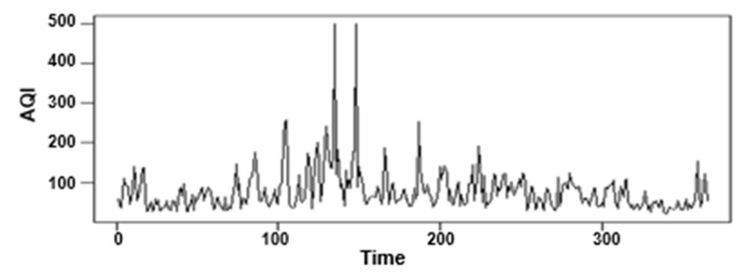
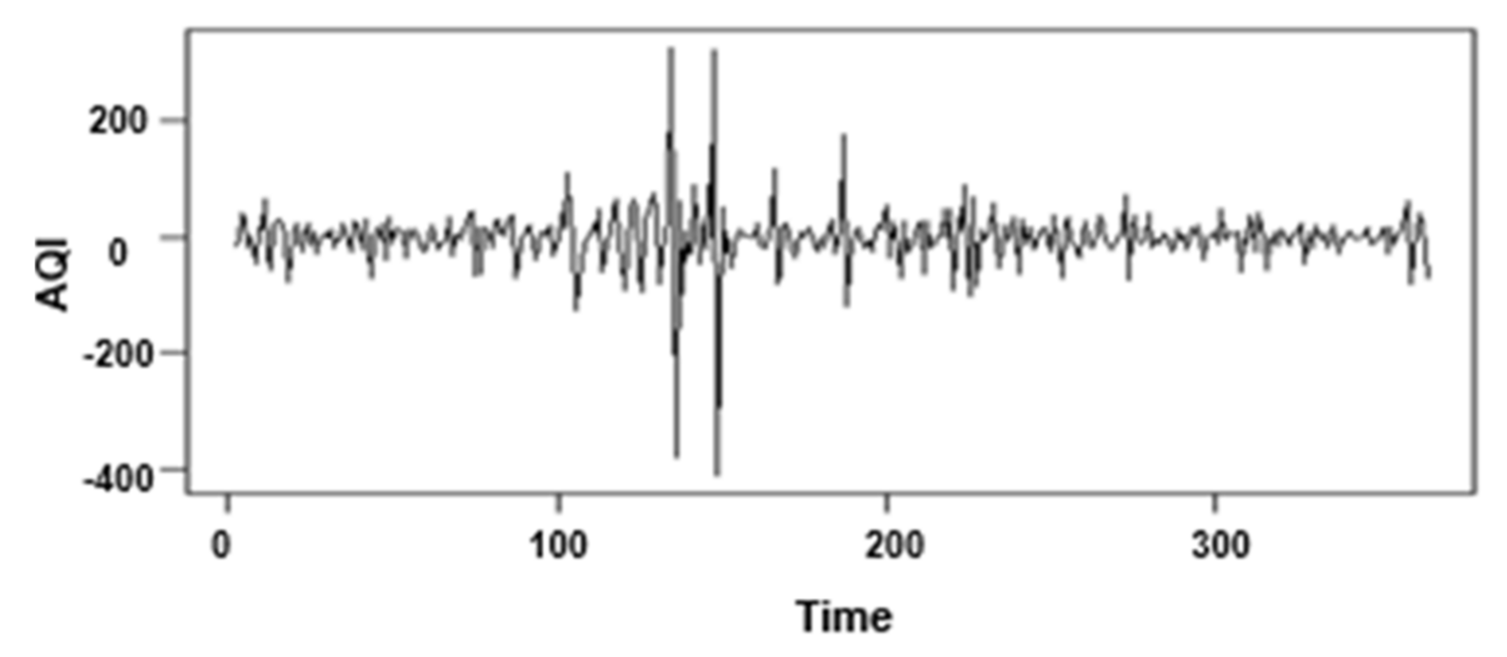
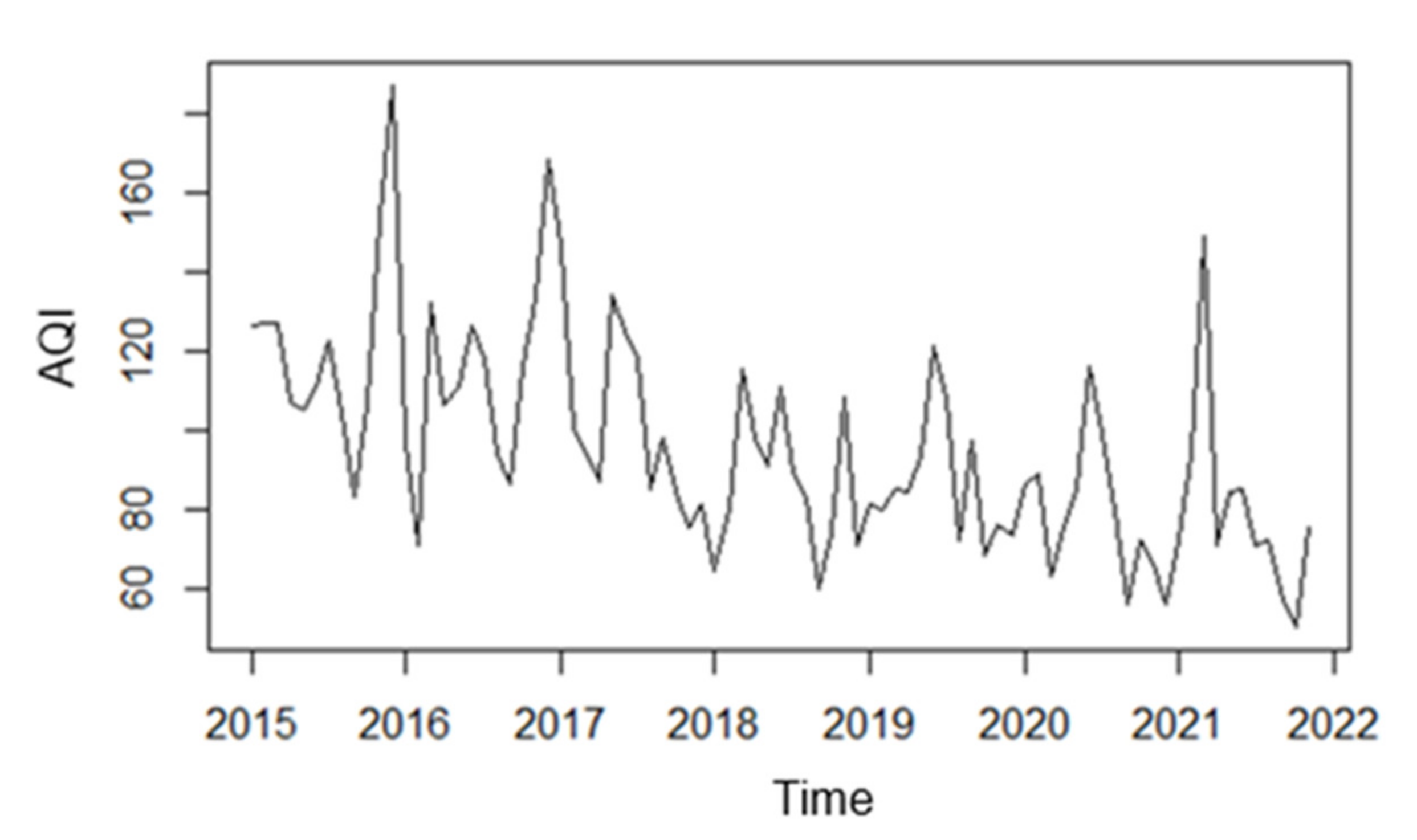
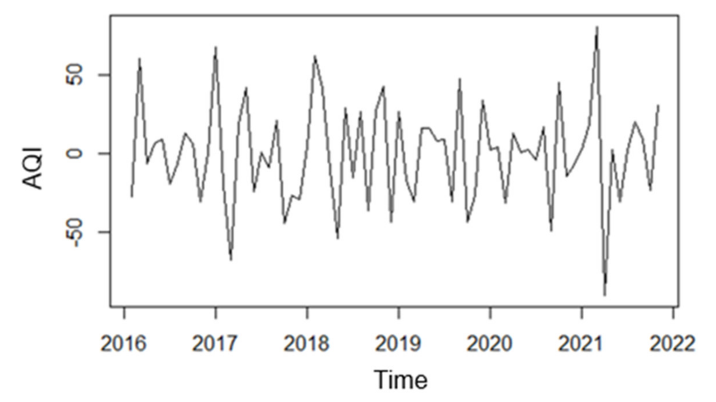
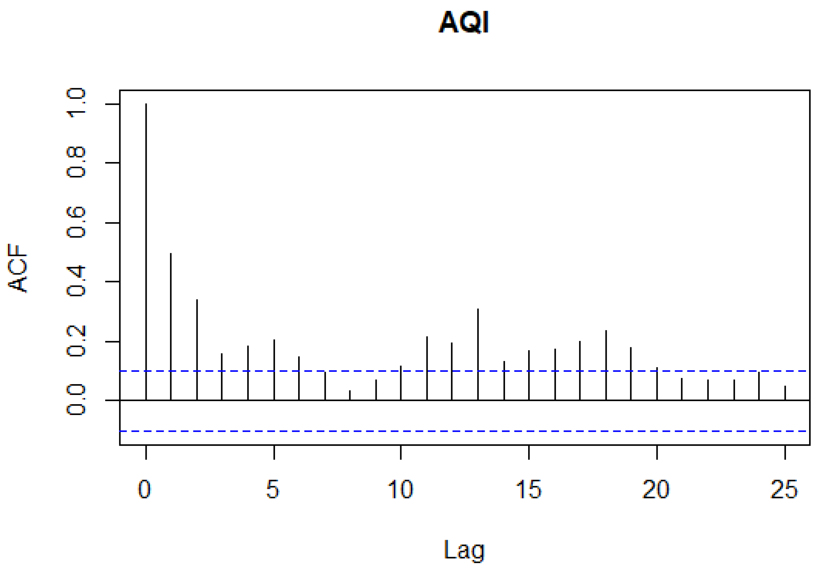
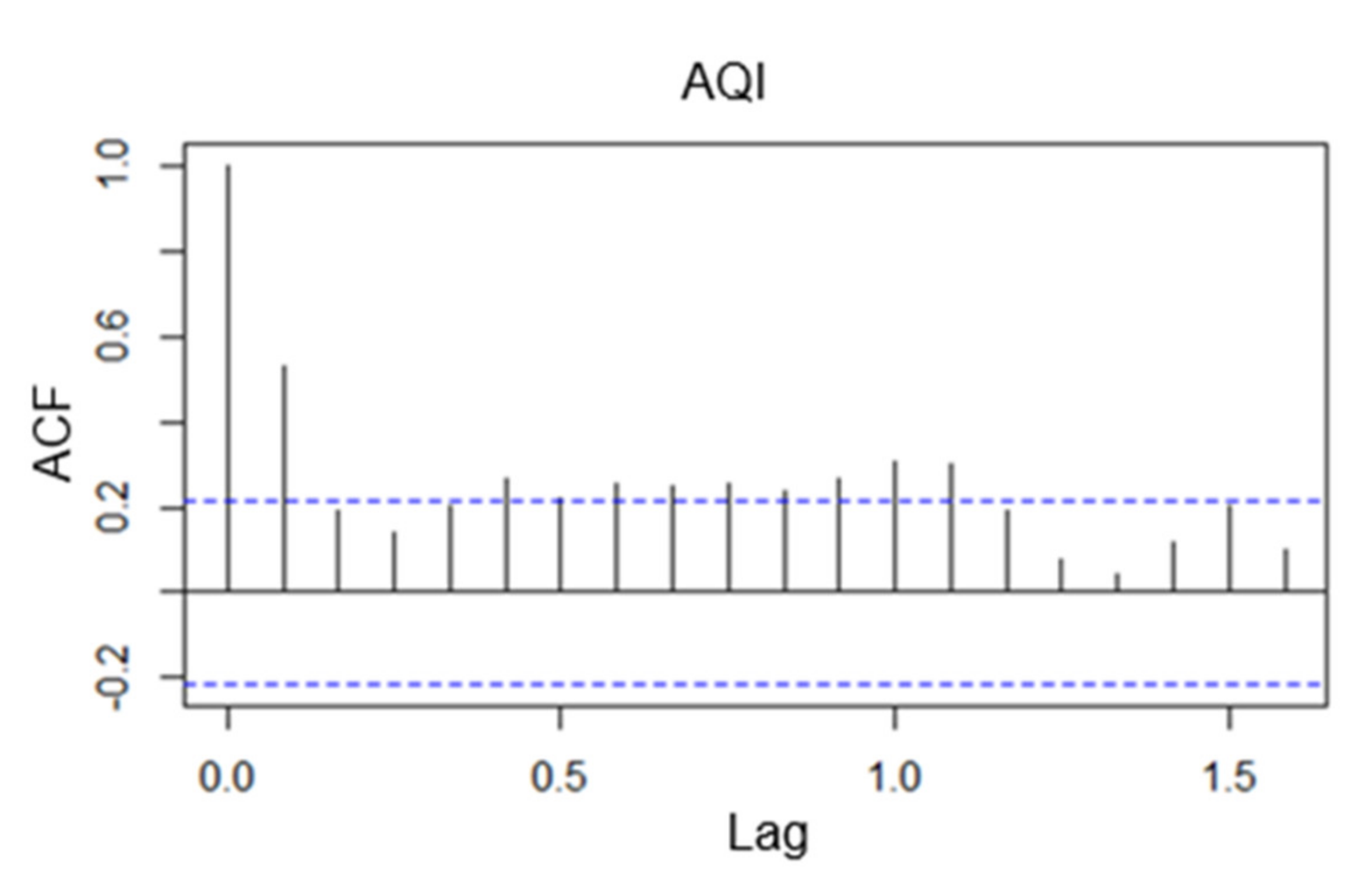
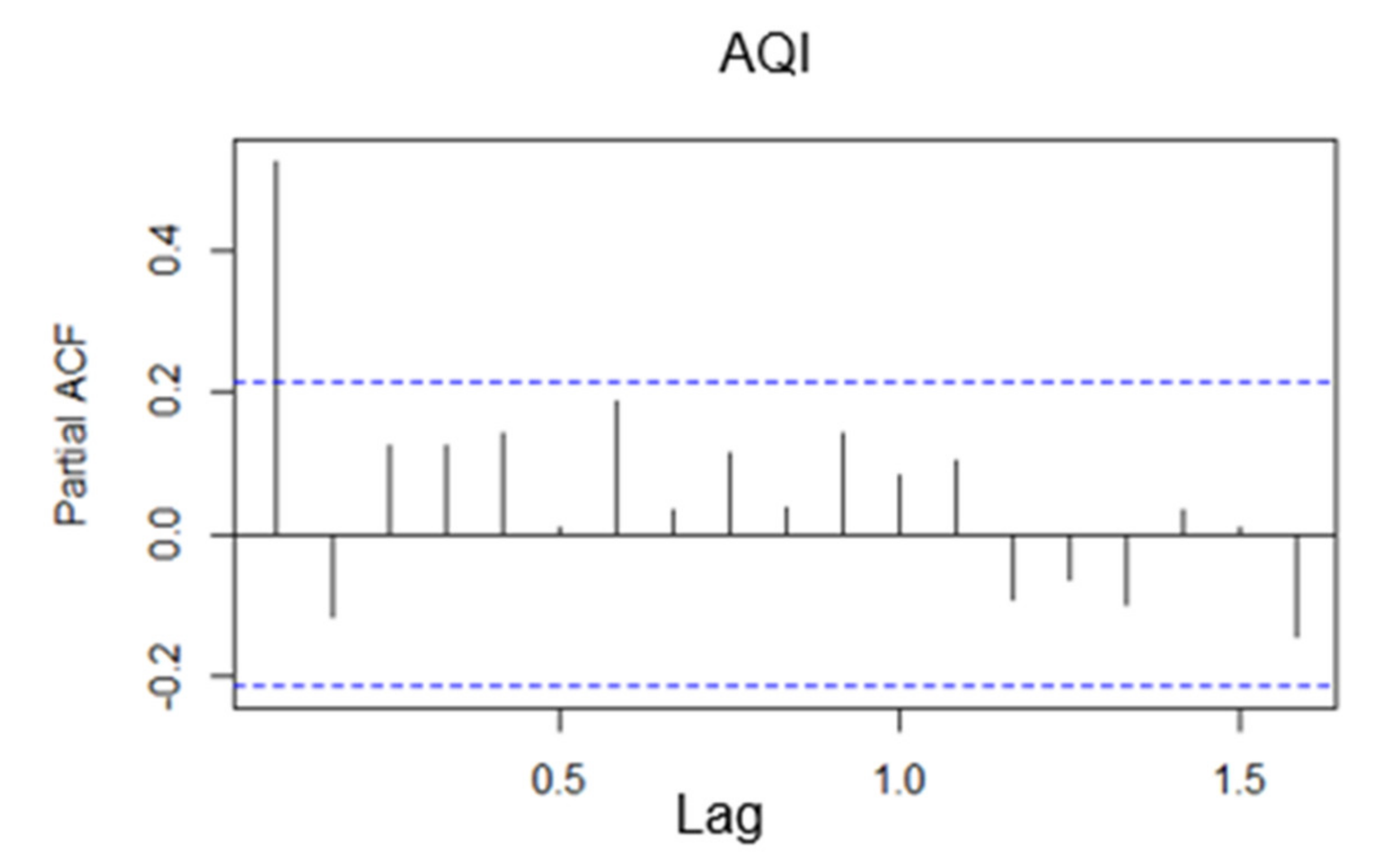
The time series plot of the AQI monthly data is drawn using R software, as Figure 20 shown below. From the time series plot of the monthly data, it is known that from January 2015 to November 2021, the overall AQI of Beijing shows a decreasing trend and has a more obvious seasonal effect. 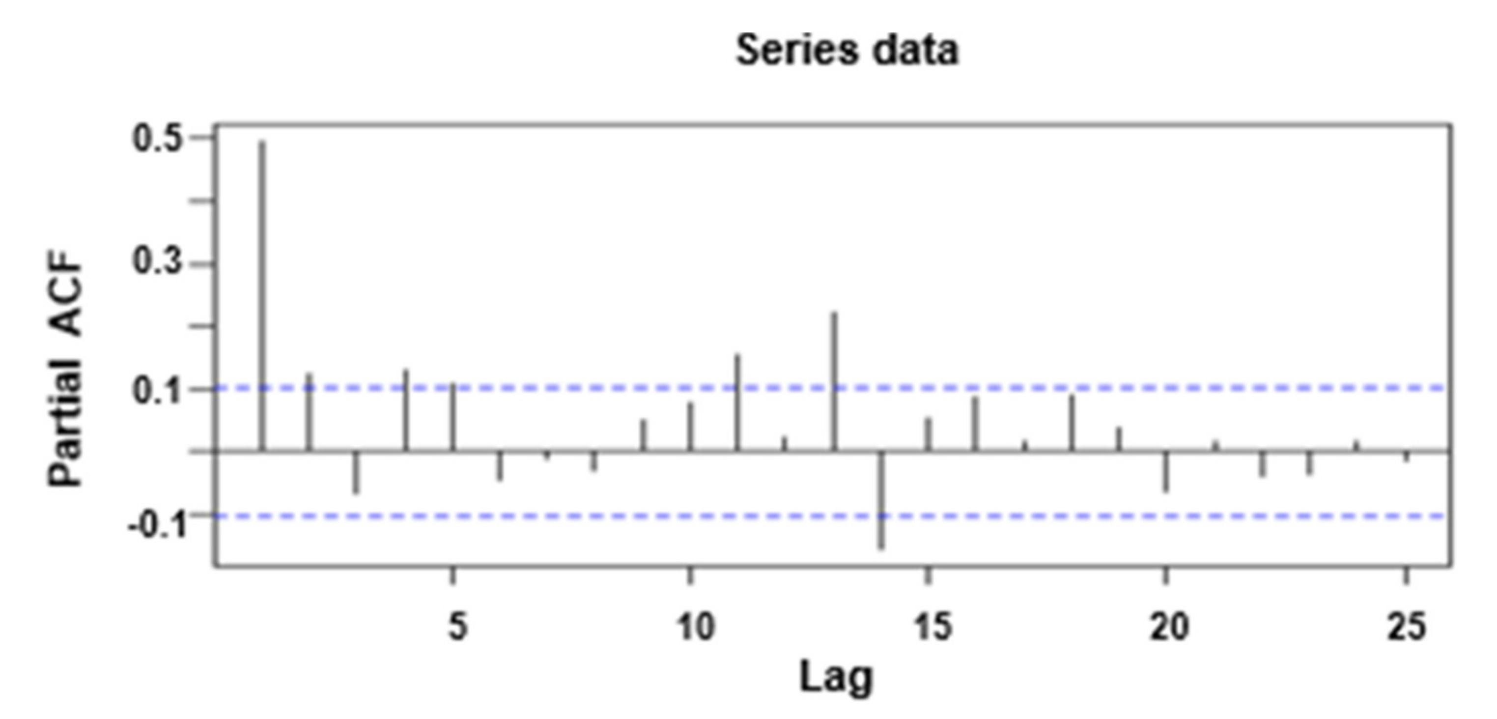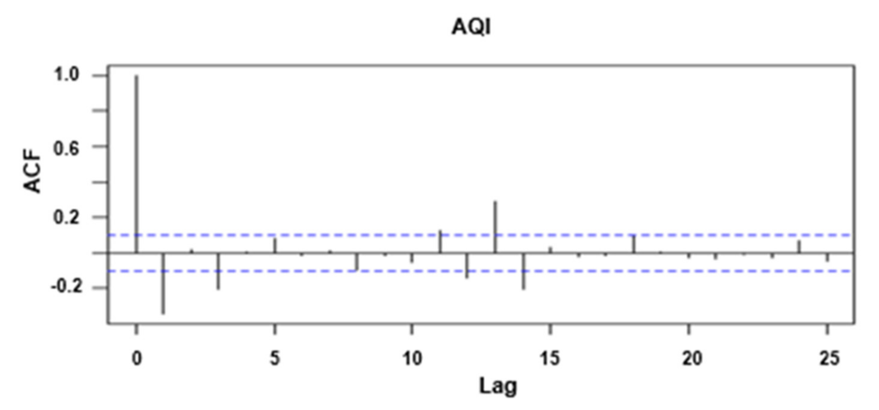Subsequently, the graphical test of autocorrelation and partial autocorrelation coefficients was conducted, as shown in Figure 21 and Figure 22, and its autocorrelation coefficients have a long-term trailing and periodic trend, and the monthly data of Beijing air quality index is initially inferred to be unsteady by the graphical test observation, and in order to further evaluate objectively the steadiness, the series is concluded to be a non-steady time series after unit root test using R software.

(2)

Pure randomness test

Similar to the ARIMA model for short-term forecast of AQI daily data, a pure randomness test is performed on the original series before the modeling analysis in order to investigate whether there is any correlation between the series and whether there is value for further study. The pure randomness test was performed using the Box.test function in the R software, and the results are shown in

Table 6. Results of pure randomness test.

Delayed Orders	p-Value
Delayed by 6 periods	2.754 × 10−7
Delayed by 12 periods	3.188 × 10−11

. It can be seen that the p-values of delayed 6 periods and delayed 12 periods are significantly less than 0.05; therefore, the original hypothesis is rejected, and the monthly data series of Beijing AQI is not a white noise series, which can be used for subsequent modeling analysis.

4.2. Construction of Seasonal Model

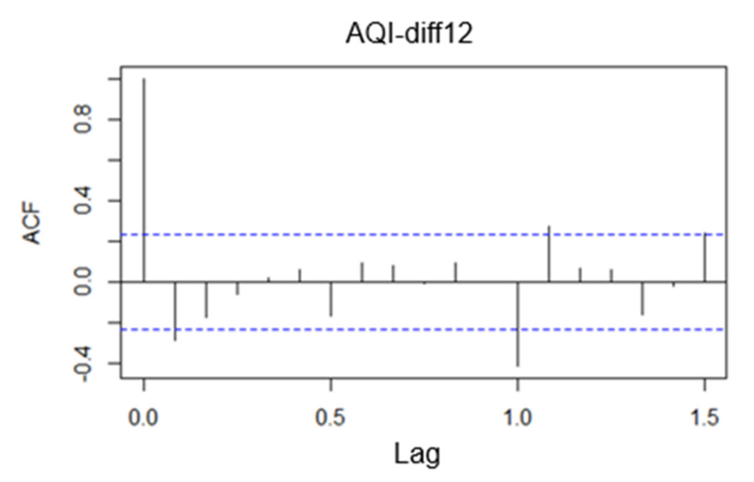
From the above time series graph, we can see that the original series shows the change of year as the cycle, and the selected air quality data is monthly data, so the cycle length s = 12. To make the original time series smooth, we need to eliminate the linear trend and seasonal periodicity of the series. Therefore, the monthly AQI data of Beijing are first differenced to eliminate the linear trend, and then differenced to eliminate the seasonal periodicity in 12 steps. 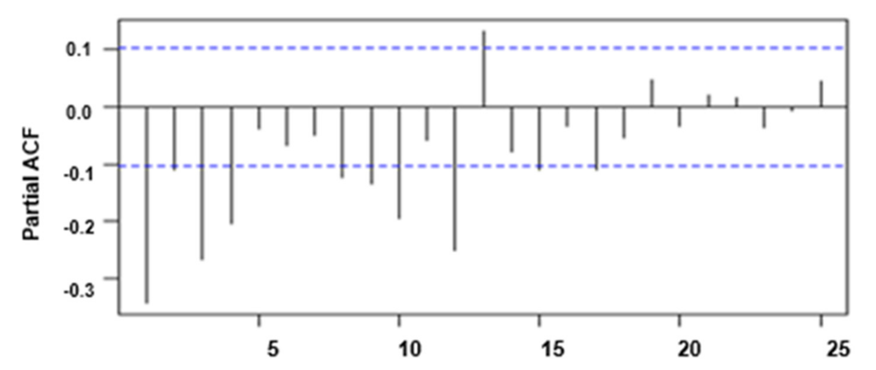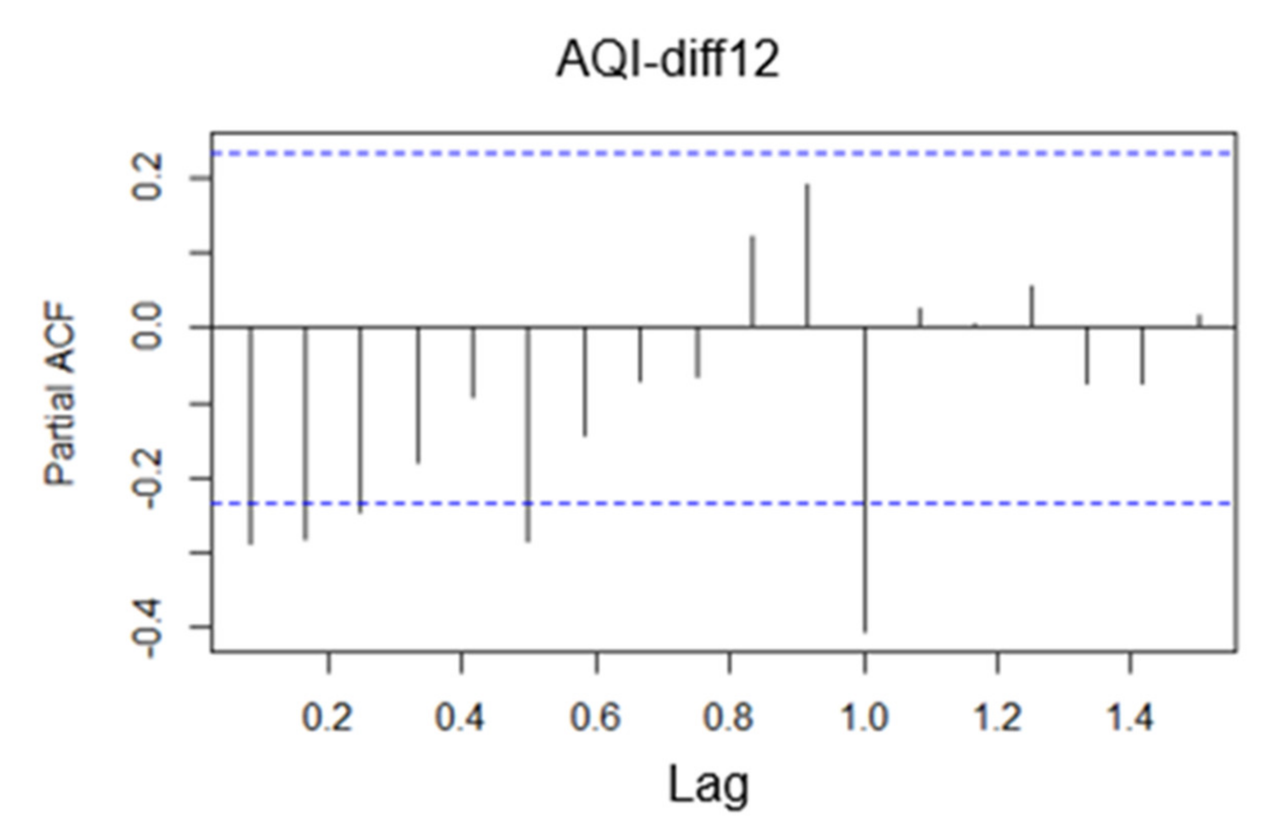The series after the first-order twelve-step differencing is denoted as AQI-diff12, and its time series is plotted as shown in Figure 23. The series after trend differencing and seasonal differencing has no obvious upward or downward trend and no obvious periodicity, fluctuating around the zero value, which can be initially judged as a smooth time series after differencing. The autocorrelation coefficients and partial autocorrelation coefficients of the series after differencing are verified by the graph test method, as shown in Figure 24 and Figure 25. The autocorrelation coefficient quickly decays to zero, and the p-value of the pure randomness test of the differenced series is 0.01, which is smaller than the significance level of 0.05. The original hypothesis is rejected, indicating that the series is smooth after eliminating the linear trend and seasonal trend. The p-value of the differenced series after the pure randomness test is 0.019, which is less than the significance level of 0.05. Therefore, the differenced series is still a non-white noise series, and the next modeling analysis is conducted for this series.

(1)

Model identification and model ranking

Based on the above autocorrelation and partial autocorrelation plots after differencing, the first step is to consider the characteristics of the autocorrelation coefficients and partial autocorrelation coefficients within 12 orders of the series after trend differencing and seasonal differencing in order to determine the short-term correlation model. In the autocorrelation and partial autocorrelation plots of the differenced series, the autocorrelation coefficients and partial autocorrelation coefficients up to order 12 are not truncated, so an ARMA(1,1) model is attempted to extract the short-term autocorrelation information of the differenced series.

The second step considers the autocorrelation characteristics of the season in question in order to confirm the choice of additive or multiplicative seasonal model. The approach is to consider the characteristics of autocorrelation coefficients and partial autocorrelation coefficients in autocorrelation plots and partial autocorrelation plots with delayed 12th order, 24th order, etc. with the length of the period as the unit. According to the autocorrelation and partial autocorrelation plots, the autocorrelation coefficients and partial autocorrelation coefficients of the delayed 12th and 24th orders fall within the range of 2 times the standard deviation, and the corresponding values of the delayed 24th order are smaller, which shows that there is no significant seasonal effect in the differenced series, so we initially consider a simple seasonal model, i.e., an additive seasonal model. At this point, the seasonal differencing order D = 1, p = 0, and Q = 0.

Combined with the previous first-order twelve-step differencing information, the additive seasonal model fitting ARIMA (1,(1,12),1) was finally determined, and its model structure is as follows.

$${\nabla }_1{\nabla }^1{x}_t=\frac{(1-{\theta }_{1}B)}{(1-{\varphi }_{1}B)}{\epsilon }_t$$

(5)

(2)

Parameter estimation of the model

The final fitted model has been determined in the previous step of the analysis, and the next step is to determine the caliber of this model based on the observed values of the series, which means that the values of the unknown parameters in the fitted model need to be estimated. Using R software, the parameters of the fitted additive seasonal model were estimated according to the maximum likelihood estimation method, and the following results were obtained, as shown in

Table 7. Estimated values of parameters.

Parameter	p-Value	Standard Deviation
${\widehat{\varphi }}_1$	0.2895	0.1163
${\widehat{\theta }}_1$	−1.0000	0.0501

.

Based on the above results, the caliber of the fitted additive seasonal model can be seen as

$${\nabla }_1{\nabla }^1{x}_t=\frac{(1+B)}{(1-0.2895B)}{\epsilon }_t$$

(6)

where $B$ is the delay operator and ${\epsilon }_t$ is the white noise sequence, i.e., ${\epsilon }_t\sim WN(0,{\sigma }^2)$.

(3)

Model testing

A white noise test of the residuals was performed on the established additive seasonal model in order to determine the significance of the model. Next, the Box.test function in the R software was used to test whether the residual series is a white noise series, and the test results are shown in

Table 8. White noise test.

X-Squared	df	p-Value
2.0741	6	0.9128
18.393	12	0.1043

. According to the results of the white noise test of the residuals, the p-value corresponding to the LB statistic at each order of delay is significantly greater than the significance level of 0.05; therefore, it can be considered that the residual series of the fitted additive seasonal model is a white noise series, which means that the established model is significantly valid.

4.3. Forecast Analysis of the Additive Seasonal Model

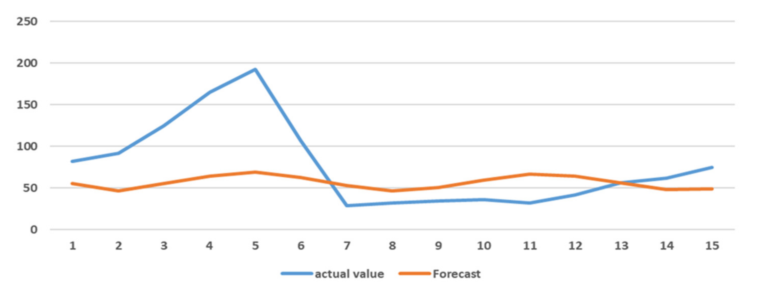
Based on the established additive seasonal model, the Beijing air quality index from December 2021 to February 2022 was selected as the test set to verify whether the model had a more accurate fit. Using the same short-term correlation criteria as above, the results are shown in

Table 9. Model goodness of fit.

Model	MAE	RMSE	MAPE	SMAPE
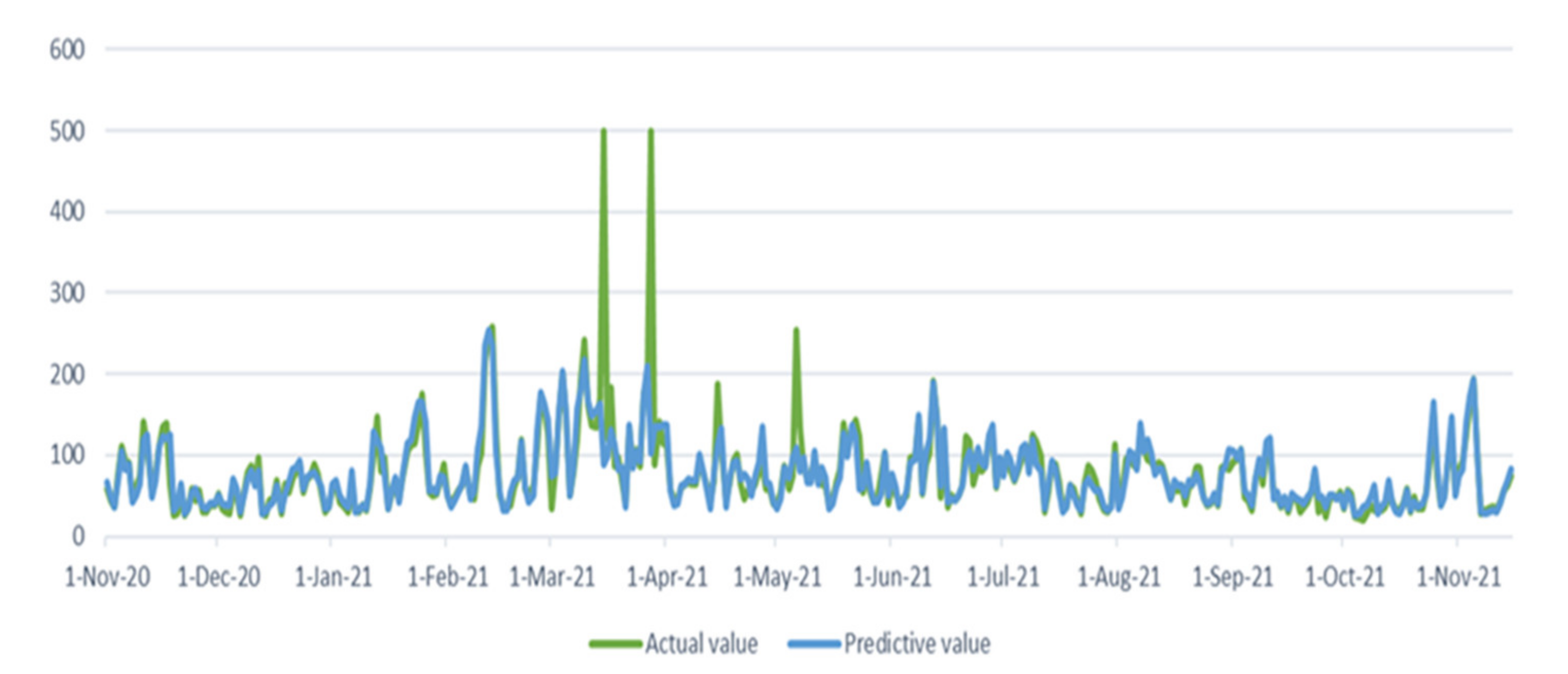
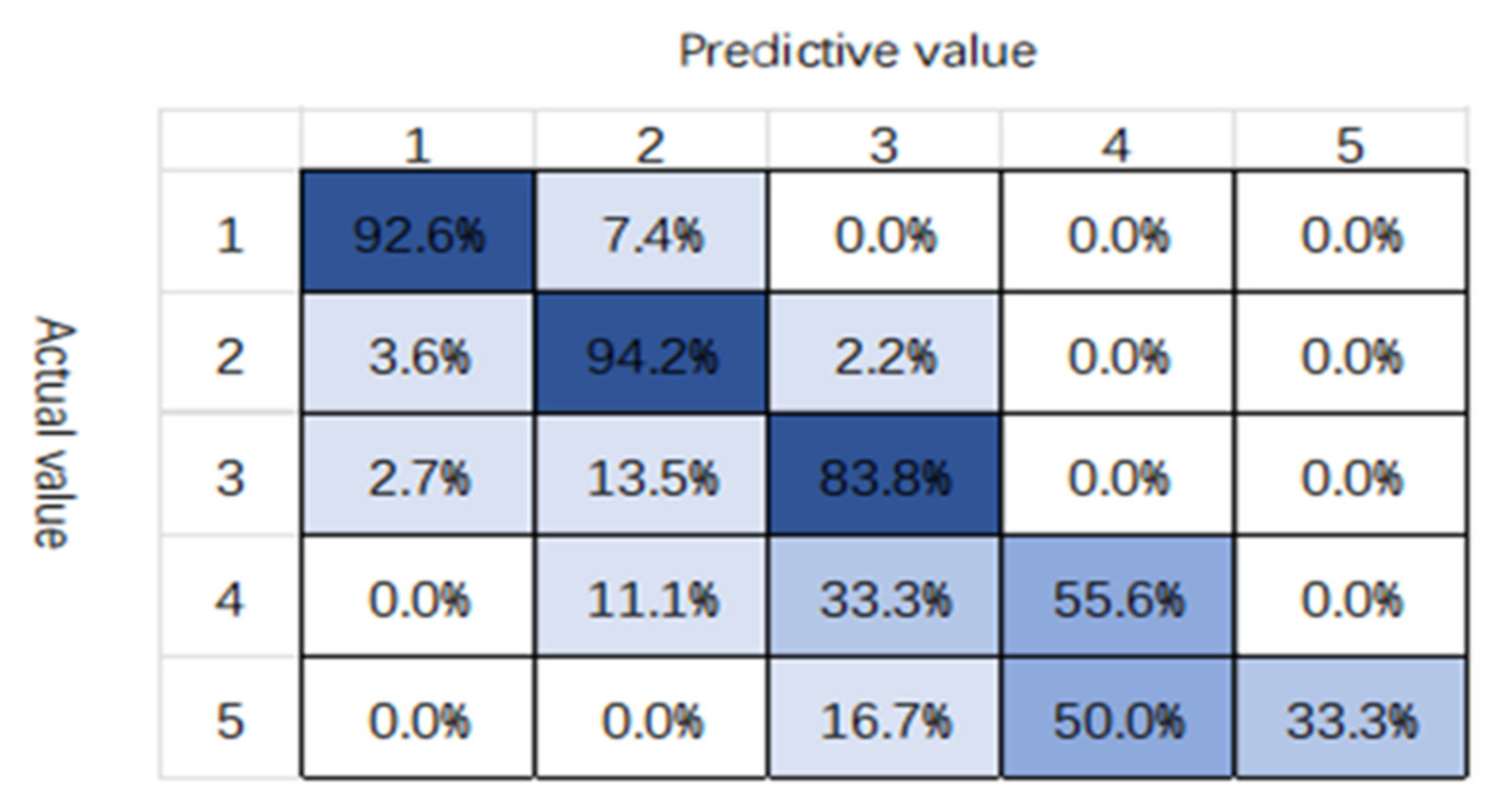
ARIMA (1,(1,12),1)	15.55	24.87	34.57%	23.89%

. As can be seen from the graphs, the differences between the predicted and true values are small and the error values are within acceptable limits, indicating that the additive seasonal model is appropriate and valid for extrapolating the future long-term Beijing AQI, with high forecast accuracy and reasonable and credible results.

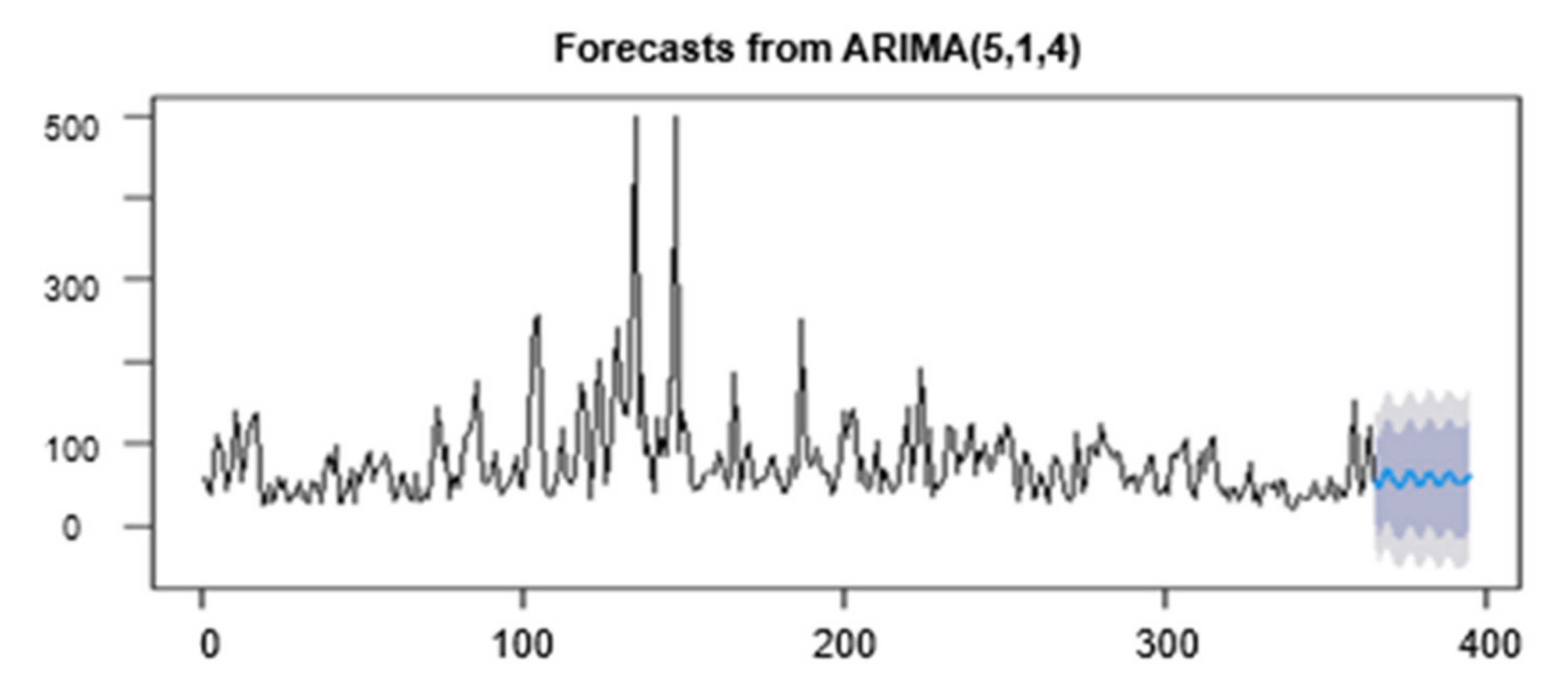
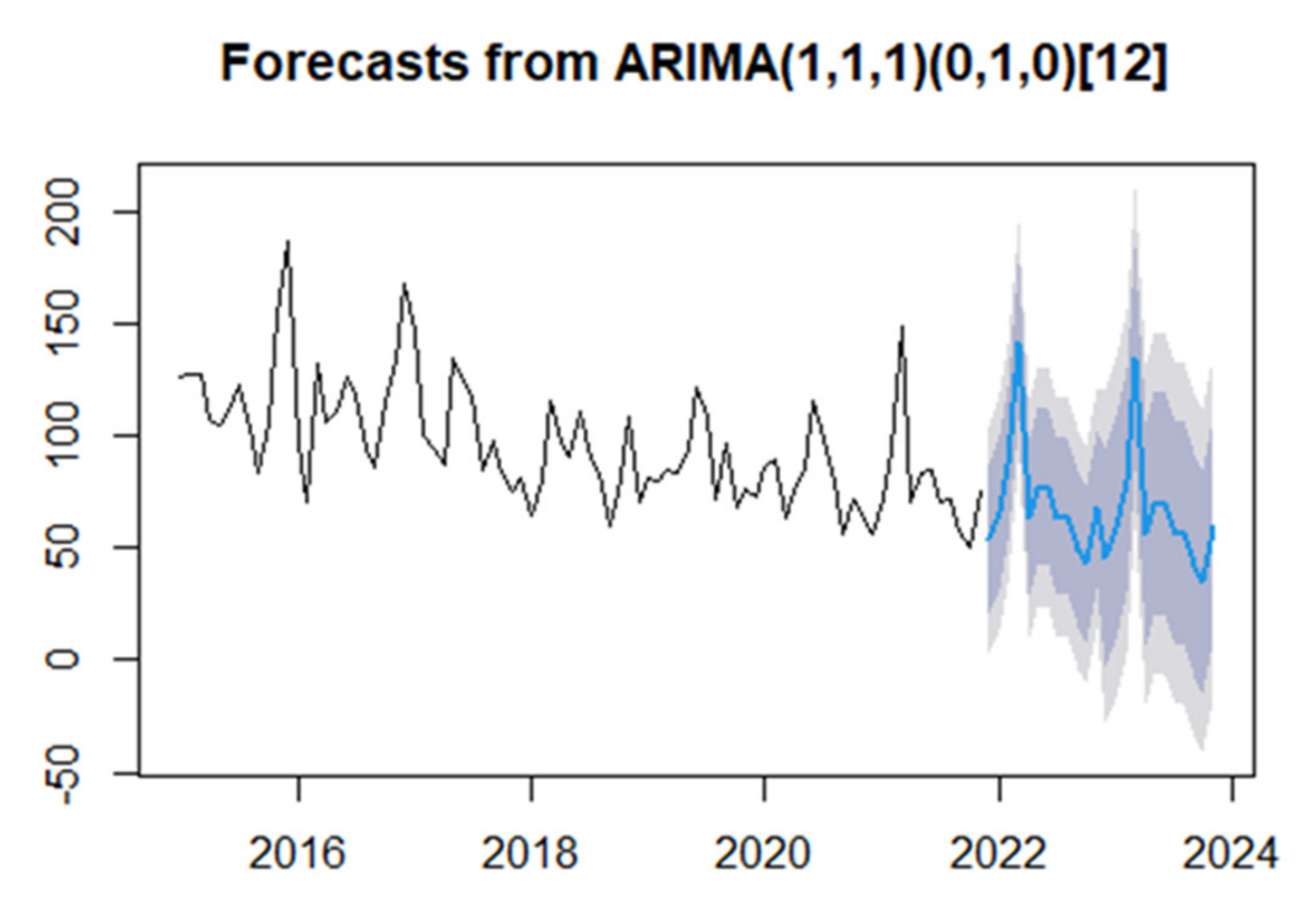
The predicted results of Beijing AQI for the next 24 periods are shown in Figure 26. It is observed that the AQI index still shows seasonal cycles and still has a slightly decreasing trend in the next two years.

4.4. Section Subsection

In this section, the long-term forecast of AQI in Beijing is based on the seasonal model of ARIMA model, which shows an overall decreasing trend of AQI in Beijing from January 2015 to November 2021 with a more obvious seasonal effect. The parameters of the fitted additive seasonal model are estimated according to the maximum likelihood estimation method, and the AQI of Beijing from December 2021 to February 2022 is predicted according to the additive model, and the results show that the AQI still shows a seasonal cycle and still has a slightly decreasing trend in the next two years.

5. Summary and Outlook

Based on Beijing’s AQI from January 2019 to November 2021 and the daily average and monthly data of six major air pollutants, this article uses descriptive statistical analysis, correlation analysis, and cluster analysis to visualize air quality development trends; Using time series analysis and data mining algorithms to build models and make short-term forecasts of Beijing’s air quality, the following conclusions are obtained:

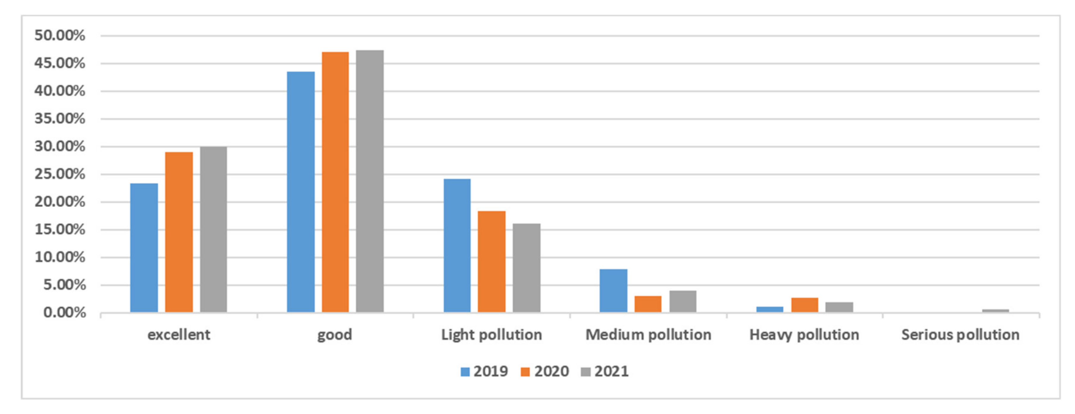
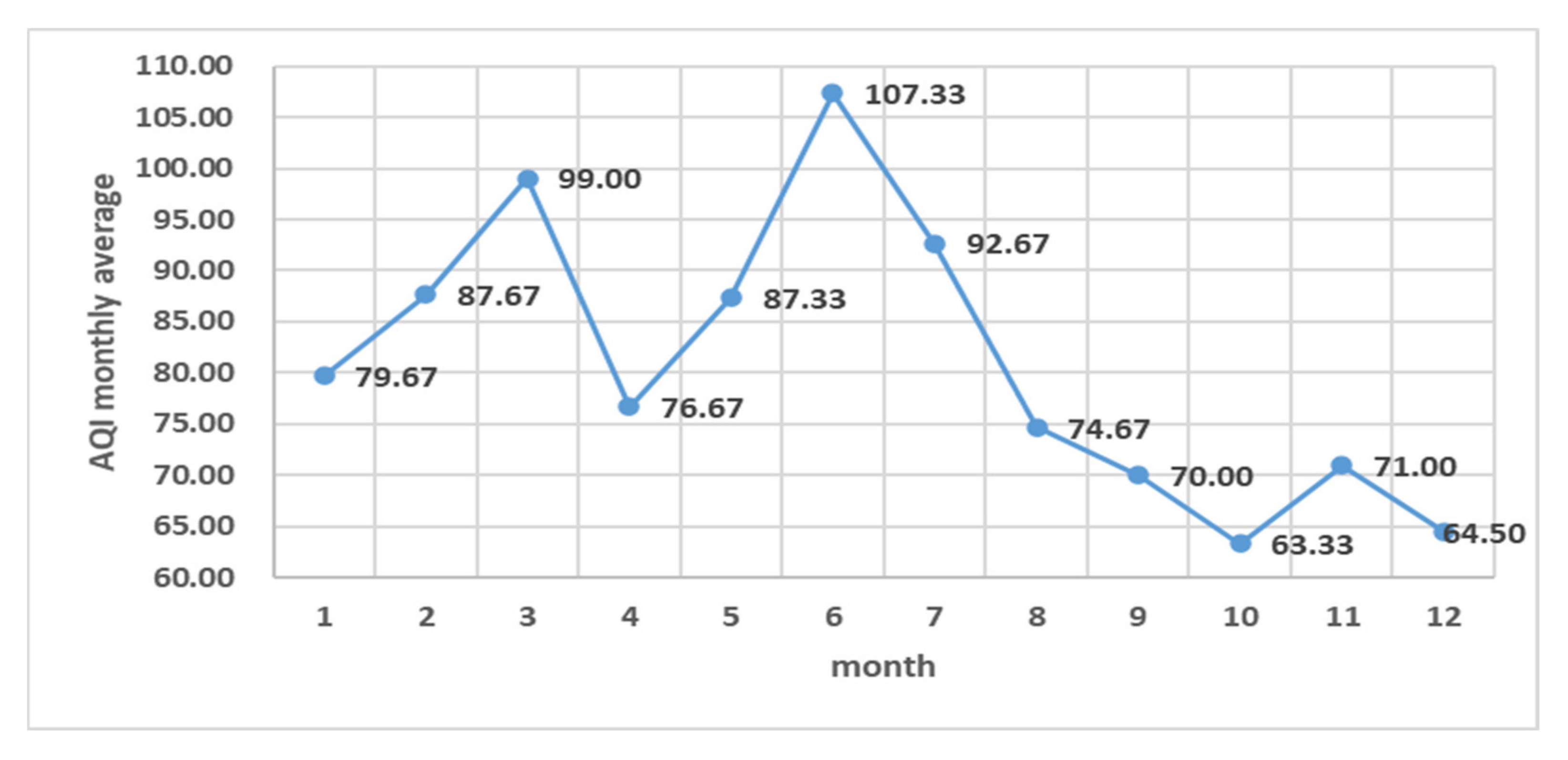
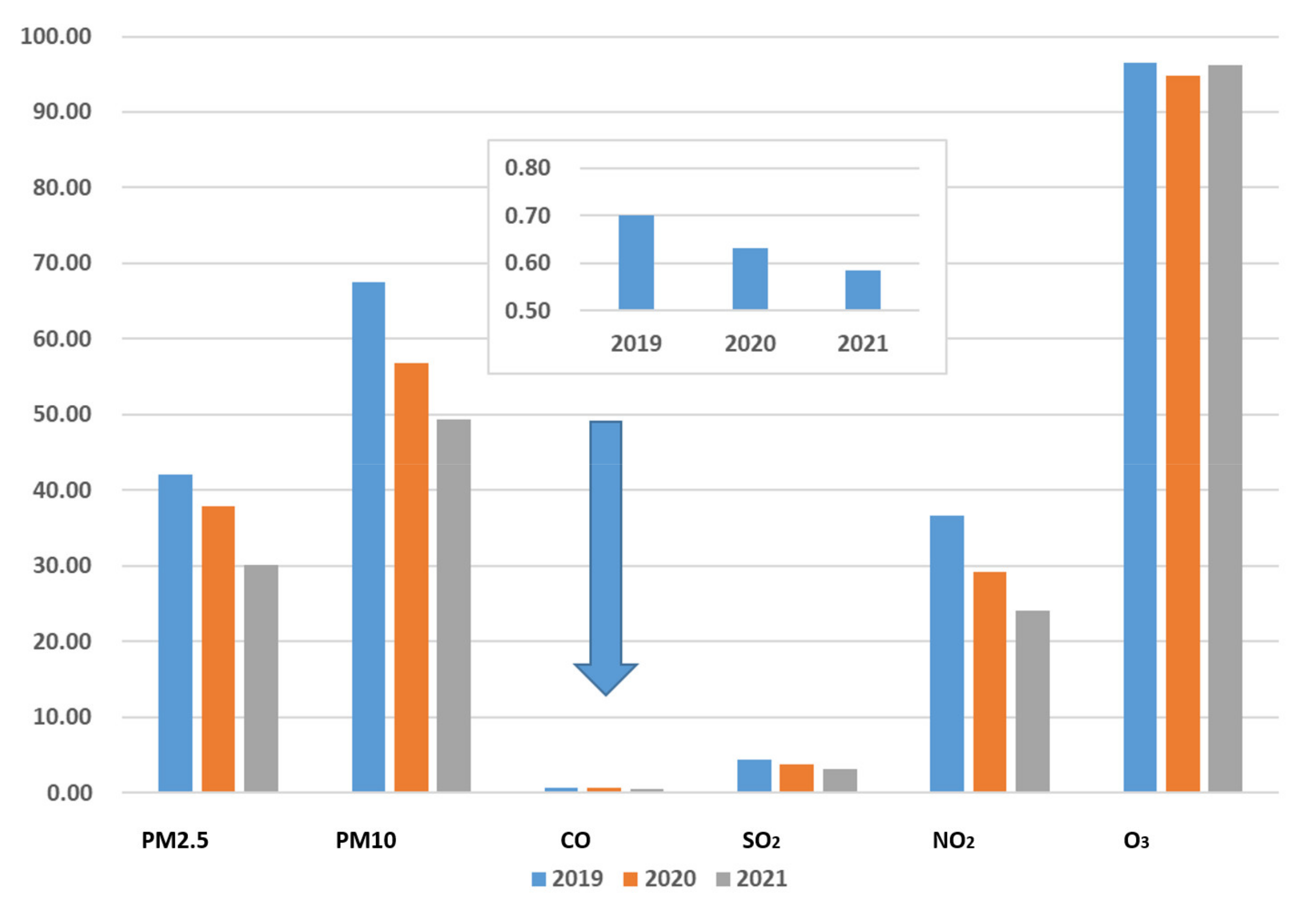
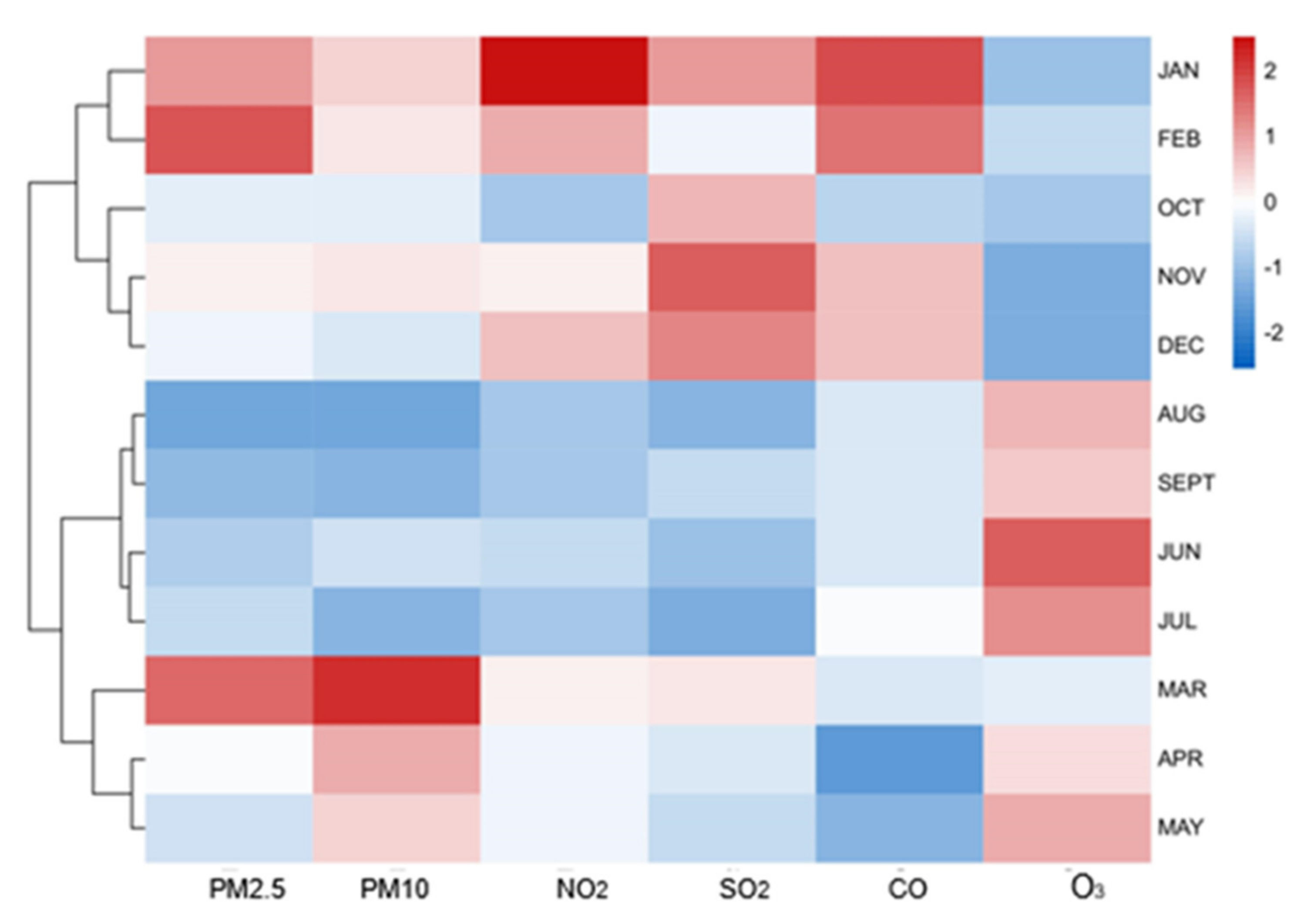
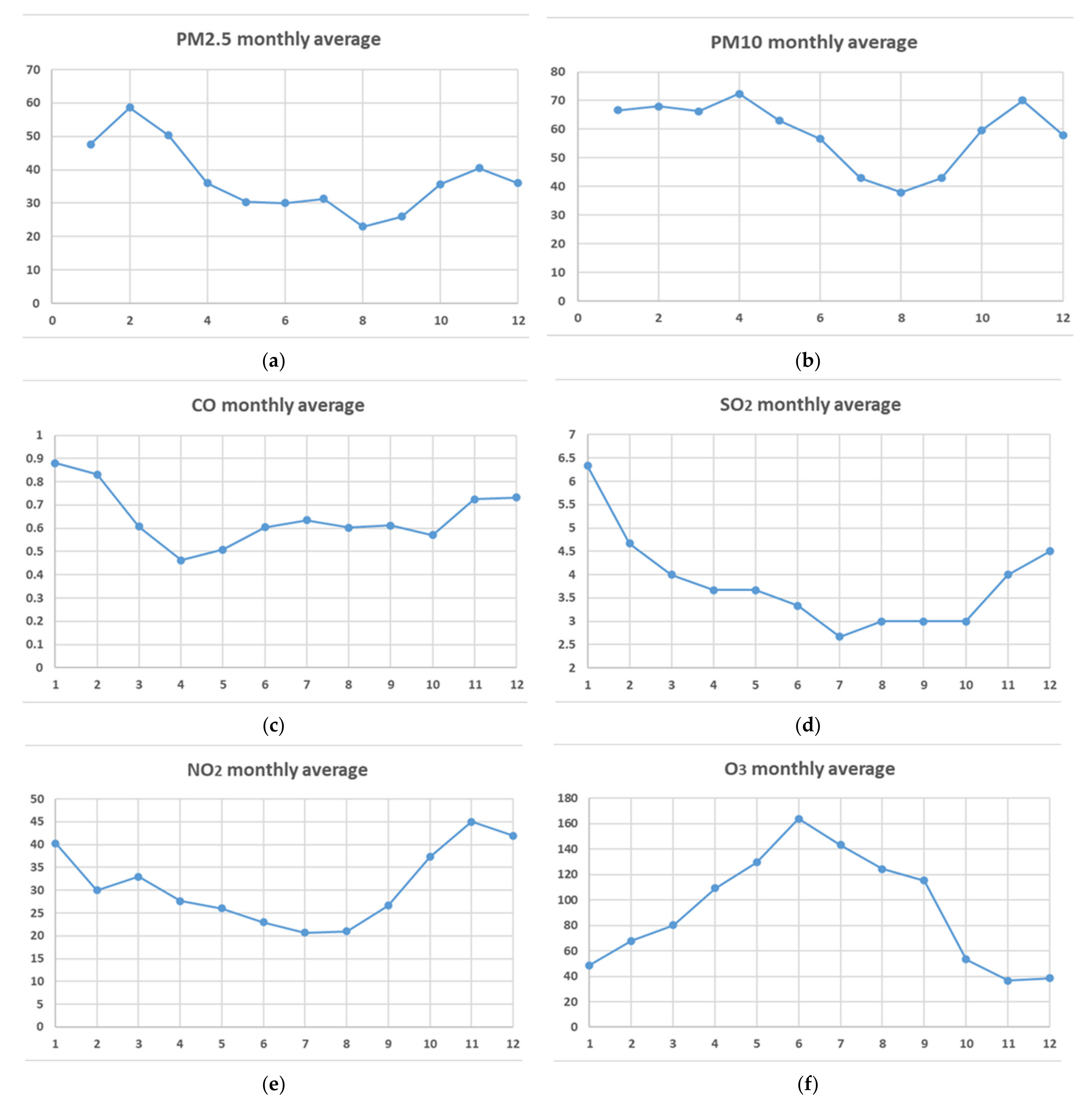
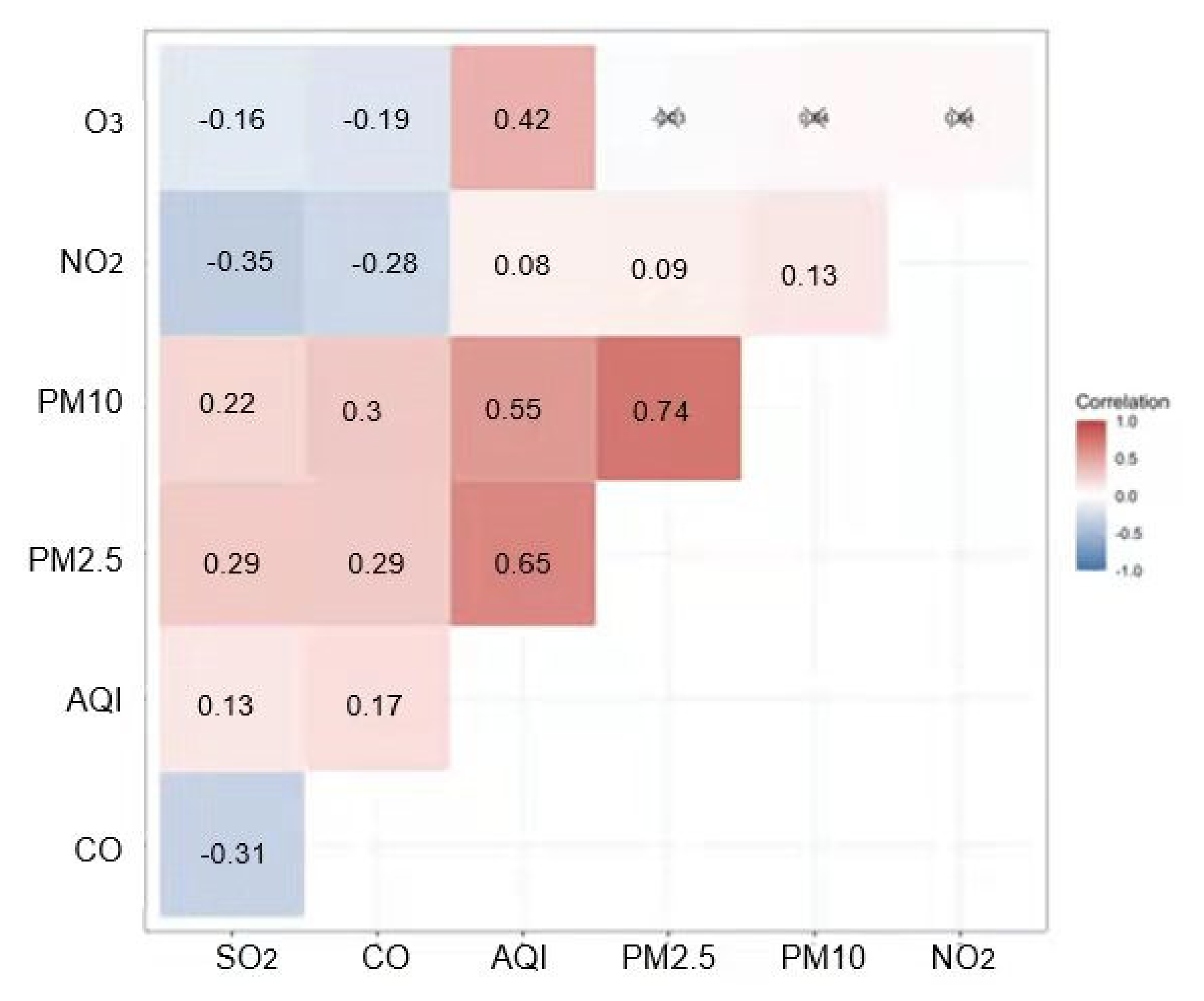
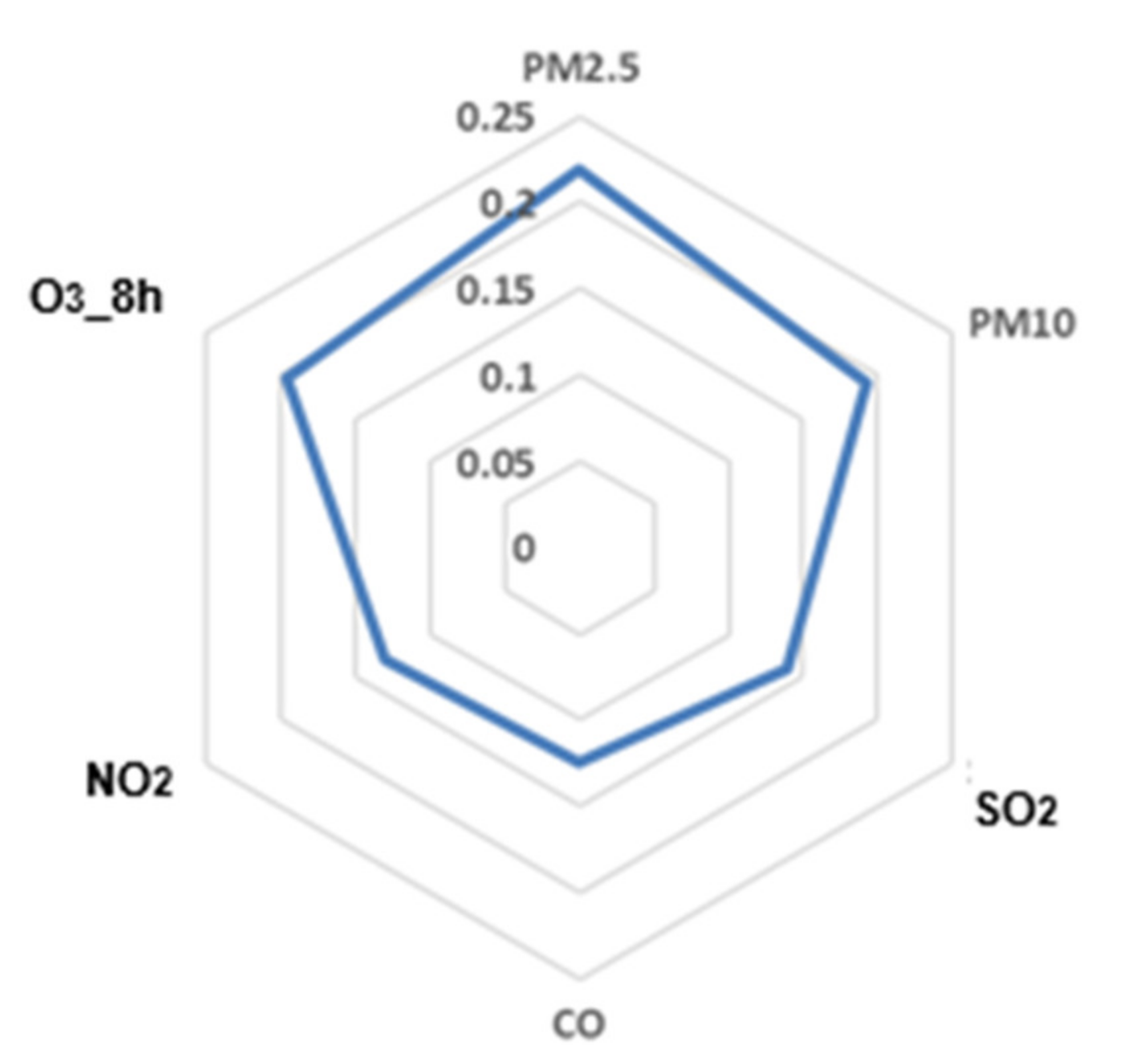
Using statistical methods to analyze the air quality level, AQI and the distribution of the six types of pollution concentration changes, the daily analysis results show that with the continuous deepening of air pollution prevention and control work, the air quality in Beijing continues to improve, AQI has improved significantly, and the level is excellent. The proportion of days has increased year by year. The monthly analysis results show that in the past three years, the air pollution level was the most serious in June, which was mainly related to the serious excess of ozone content. The changes in air quality in Beijing show obvious seasonal characteristics. The five main pollutants PM2.5, PM10, SO₂, CO, and NO₂ have low concentrations in summer and high concentrations in winter; only O₃ is the opposite of other pollutants. Because of the high concentration in summer and low concentration in winter, the persistently high content of ozone is still a thorny issue facing today, and the air quality varies greatly between the heating period and non-heating period.

The short-term forecast of Beijing air quality index using time series model and neural network model overcomes the lag of the current air quality monitoring system, and the AQI index high and low is determined by the co-construction of six air pollutants. The results show that both ARIMA model and neural network model are significant for the forecast of air quality index, and the established models are reasonable and effective, and it is found by comparison, the fitting effect of the neural network is better than that of the ARIMA model, but both models have their own characteristics. It was also found that PM2.5, PM10, and O₃ have a greater influence on the air quality class, and are the main factors to determine the specific value of AQI and air quality class. When using the additive seasonal model for long-term forecast of monthly data, it was found that the Beijing AQI still shows seasonal cyclicality and still has a slightly decreasing trend in the next two years. In summary, based on the conclusions of the article, we can propose measures to improve air quality from the three perspectives of the government, society, and individuals.

The government must increase implementation of environmental protection policies and investment in environmental protection technology. Environmental protection departments should strengthen environmental management, earnestly implement national and local laws and regulations, comprehensively use technical means and administrative measures, and manage air quality through legislation, monitoring, and protection.

The analysis shows that PM2.5, PM10, and O₃ have a greater impact on air quality levels. Therefore, environmental protection management agencies have been established at all levels from the central to the local level to use monitoring technology tools to publish monitoring data promptly, inspect and dispose of pollution sources, and control building dust, Pollution behaviors such as burning coal for heating and burning straw. Increase investment in the field of environmental protection technology, develop reasonable treatment equipment, reduce waste of resources, and improve sewage treatment technology. Optimize the industrial structure, lower pollution standards, and increase pollution punishment. Resource control policies such as pollutant discharge fees have a significant impact on pollution control costs. The development of a washing energy industry with high energy utilization and low pollution, and making good use of renewable resources such as solar and wind energy. Air pollution has fluidity and regional characteristics, and its changes are synchronized. Pollution between regions affects each other. Pollution prevention and control is not just an administrative region’s problem. It is necessary to establish a regional cooperation system, regional joint prevention and control, to solve cross-regional air pollution problems, for example, the Beijing-Tianjin-Hebei simultaneous implementation of the “Regulations on the Prevention and Control of Emission Pollution from Motor Vehicles and Non-road Mobile Machinery”, and so on. Improve urban green coverage, borrow the characteristics of plants to absorb dust and purify the air, provide zoning control strategies for the in-depth fight against pollution, and continue to promote precise, scientific, and legal pollution control.

The society must vigorously promote environmental protection knowledge, raise awareness of protecting the atmospheric environment, and advocate low-carbon life. Prevention and control work increasingly requires scientific and refined management. The city should adhere to project emission reductions and management emission reductions according to changes in air quality in months and seasons, and promote the formation of a spatial pattern, industrial structure and lifestyle that conserves resources and protects the environment. The aims are to deepen the “one microgram” action, focus on the coordinated governance of PM2.5, PM10 and O₃, and achieve green transformation of the industrial structure, green and low-carbon energy structure, green optimization of vehicle structure, and green and clean urban appearance.

Another aim is to establish an action pattern led by the government and public participation. With the expansion of the scale of cities and the improvement of the level of economic activities, the number of motor vehicles has increased, and cars emit a large amount of NO₂ and inhalable particulate matter, which will seriously damage the environment and affect people’s health. Therefore, it is necessary to consciously eliminate old motor vehicles and improve awareness of the purification and treatment of polluting vehicle exhausts, supporting the development and use of new energy vehicles. The general public should actively participate in environmental protection activities and environmental protection supervision, consciously practice a simple and moderate, green and low-carbon lifestyle, and offer advice and suggestions for a more beautiful Beijing.

References

1. Wu, J.; Yang, Z.H.; Hu, L. Study on the benefits of urban eco-spatial air quality improvement based on spatial dependence—Beijing as an example. China Environ. Sci. 2021, 1–10. [Google Scholar] [CrossRef]
2. Ma, T. Analysis and Prediction of AQI in Jinan; Shandong University: Jinan, China, 2021. [Google Scholar] [CrossRef]
3. Zhang, X.; Luo, S.; Li, X.; Li, Z.; Fan, Y.; Sun, J. Temporal and Spatial Variation Characteristics of Air Quality in China. Sci. Geogr. Sin. 2020, 40, 190–199. [Google Scholar]
4. Xiao, Y.; Tian, Y.; Xu, W.; Liu, J.; Wan, Z.; Zhang, X.; Liu, X. Characteristics of Urban Air Pollution and its Socio-economic Impact in China. Ecol. Environ. Sci. 2018, 27, 518–526. [Google Scholar]
5. Guo, W.; Chen, Y.; Liu, G.; Song, K.; Tao, B. Analysis on the Characteristics and Influencing Factors of Air Quality of Urban Agglomeration in the Middle Reaches of the Yangtze River in 2016 to 2019. Ecol. Environ. Sci. 2020, 29, 2034–2044. [Google Scholar]
6. Liu, Y.; Zhang, Y.; Zhu, C.; Hao, J.; Liu, Q. Intelligent Forecasting and Monitoring of Air Index Based on Big Data and Internet of Things. J. Commun. 2017, 38, 129–138. [Google Scholar]
7. Zhou, M.; Yang, Y.; Sun, Y.; Zhang, F.; Li, Y. Analysis of air quality spatial and temporal distribution characteristics and influencing factors in Shandong Province from 2016 to 2020. Environ. Sci. 2022, 1–12. [Google Scholar] [CrossRef]
8. Ziheng, J.; Xizhang, G.; Baolin, L.; Dechao, Z.; Jie, X.; Fei, L. Analysis on the temporal and spatial distribution pattern and influencing factors of air quality in Sichuan and Chongqing areas. J. Ecol. 2022, 11, 1–10. [Google Scholar]
9. Jędruszkiewicz, J.; Czernecki, B.; Marosz, M. The Variability of PM10 and PM2.5 Concentrations in Selected Polish Agglomerations: The Role of Meteorological Conditions, 2006–2016. Int. J. Environ. Health Res. 2017, 27, 441–462. [Google Scholar] [CrossRef] [PubMed]
10. Lu, B. Application of Statistical Analysis and Machine Learning Method to Air Quality Prediction in Yinchuan City. In Engineering Science and Technology; CNKI: Beijing, China, 2021; Volume 1. [Google Scholar] [CrossRef]
11. Wang, W.; Zheng, Z.; Liang, X.; Zhou, H. Application of Grey System Model in Forecasting Ambient Environment Quality in Jinan City. J. Green Sci. Technol. 2013, 3, 123–126. [Google Scholar]
12. Dong, S.; Su, T.; Huang, L.; Lv, Z. Fuzzy Comprehensive Evaluation and Curve Fitting Prediction Models for Air Quality. Math. Pract. Theory 2018, 48, 102–108. [Google Scholar]
13. Akdi, Y.; Gölveren, E.; Ünlü, K.D.; Yücel, M.E. Modeling and forecasting of monthly PM2.5 emission of Paris by periodogram-based time series methodology. Environ. Monit. Assess. 2021, 193, 622. [Google Scholar] [CrossRef] [PubMed]
14. Wu, Q.; Lin, H. Daily Urban Air Quality Index Forecasting Based on Variational Mode Decomposition, Sample Entropy and LSTM Neural Network. Sustain. Cities Soc. 2019, 50, 101657. [Google Scholar] [CrossRef]
15. Rahimi, A. Short-term Forecast of NO2 and NOx Concentrations Using Multilayer Perception Neural Network: A Case Study of Tabriz, Iran. Ecol. Processes 2017, 6, 4. [Google Scholar]
16. Zhao, Y.; Zhang, X.; Chen, M.; Gao, S.; Li, R. Regional Variation of Urban Air Quality in China and Its Dominant Factors. Acta Geogr. Sin. 2021, 76, 2814–2829. [Google Scholar]
17. Yang, S.; Zhao, L. Application of Random Forest Algorithm in Urban Air Quality Forecast. Stat. Decis. 2017, 20, 83–86. [Google Scholar] [CrossRef]
18. Akbal, Y.; Ünlü, K.D. A deep learning approach to model daily particular matter of Ankara: Key features and forecasting. Int. J. Environ. Sci. Technol. 2021, 1–17. [Google Scholar] [CrossRef]
19. HJ633-2012; Technical Regulation on Ambient Air Quality Index (ON Trial). Ministry of Environmental Protection of the People’s Republic of China: Beijing, China, 2012.
20. Yin, C.; Li, H.; Yu, L.; Wang, A. Characteristics of Air Quality in Jinan. J. Shandong Meteorol. 2012, 32, 24–26. [Google Scholar]
Figure 1. 2019–2021 Beijing’s AQI level comparison chart.
Atmosphere 13 00512 g001
Figure 2. Visualization of the monthly average value of Beijing’s AQI 2019–2021.
Atmosphere 13 00512 g002
Figure 3. The temporal characteristics of the six pollutants in Beijing from 2019 to 2021.
Atmosphere 13 00512 g003
Figure 4. Heat map of six air pollutant indicators.
Atmosphere 13 00512 g004
Figure 5. Monthly average data of the six major pollutants in Beijing for the same period of the three years from 2019 to 2021. (a) Monthly average data of the PM2.5 concentration in Beijing for the same period of the three years from 2019 to 2021. (b) Monthly average data of the PM10 concentration in Beijing for the same period of the three years from 2019 to 2021. (c) Monthly average data of the CO concentration in Beijing for the same period of the three years from 2019 to 2021. (d) Monthly average data of the SO2 concentration in Beijing for the same period of the three years from 2019 to 2021. (e) Monthly average data of the NO2 concentration in Beijing for the same period of the three years from 2019 to 2021. (f) Monthly average data of the O3 concentration in Beijing for the same period of the three years from 2019 to 2021.
Atmosphere 13 00512 g005
Figure 6. Correlation heat map of six air pollutant indicators.
Atmosphere 13 00512 g006
Figure 7. Time series of Beijing AQI original data.
Atmosphere 13 00512 g007
Figure 8. An apocalypse coefficient plot of the original AQI data in Beijing.
Atmosphere 13 00512 g008
Figure 9. Partial correlation diagram of the original AQI data in Beijing.
Atmosphere 13 00512 g009
Figure 10. Time series diagram of Beijing’s AQI after first-order difference.
Atmosphere 13 00512 g010
Figure 11. Autocorrelation coefficient after the first-order difference of Beijing AQI.
Atmosphere 13 00512 g011
Figure 12. The partial autocorrelation coefficient after the first-order difference of Beijing AQI.
Atmosphere 13 00512 g012
Figure 13. ARIMA model predicts Beijing’s AQI map.
Atmosphere 13 00512 g013
Figure 14. Comparison of predicted value and the true value of ARIMA model.
Atmosphere 13 00512 g014
Figure 15. Absolute error histogram of ARIMA forecasting model.
Atmosphere 13 00512 g015
Figure 16. The relative error histogram of the ARIMA forecasting model.
Atmosphere 13 00512 g016
Figure 17. Neural network model forecast diagram.
Atmosphere 13 00512 g017
Figure 18. Accuracy of the classification model.
Atmosphere 13 00512 g018
Figure 19. Analysis of the importance of six air pollutant indicators.
Atmosphere 13 00512 g019
Figure 20. Time series of Beijing AQI monthly data.
Atmosphere 13 00512 g020
Figure 21. Monthly AQI series autocorrelation chart.
Atmosphere 13 00512 g021
Figure 22. Monthly data AQI bias autocorrelation graph.
Atmosphere 13 00512 g022
Figure 23. Time series of monthly AQI data after first-order twelve-step differencing.
Atmosphere 13 00512 g023
Figure 24. Autocorrelation of monthly AQI data after first-order 12-step differencing.
Atmosphere 13 00512 g024
Figure 25. Biased autocorrelation of monthly AQI data after first-order 12-step differencing.
Atmosphere 13 00512 g025
Figure 26. ARIMA model long-term forecast graph.
Atmosphere 13 00512 g026