Study on the Mechanism of Haze Pollution Affected by Urban Population Agglomeration

Abstract

Population agglomeration and haze pollution are two major problems that urban development will inevitably face in the future. Population agglomeration has a spatial impact on smog pollution through scale and intensive effects. This paper uses panel data from 236 prefecture-level cities in China from 2001 to 2012 to verify the impact of urban population agglomeration on haze pollution and its mechanism based on a spatial lag model. The research shows that: (1) China’s urban haze pollution has a significant positive spatial spillover effect, and presents a spatial distribution state of high-high and low-low agglomeration. (2) There is a significant “N-type” nonlinear relationship between urban population agglomeration and haze pollution. (3) At present, the scale effect of urban population agglomeration in China is greater than the intensification effect, and the scale effect as well as intensification effect have opposite effects on haze pollution. This shows that urban layout should be scientifically planned, urban population should be reasonably controlled, production efficiency should be improved, and green development should be promoted to deal with haze pollution. (4) The spillover effect of urban population agglomeration on haze pollution is significantly greater than the direct effect, indicating that local haze pollution is more likely to be affected by spatially related regions, indicating that strengthening regional coordination and cooperation and joint prevention and control are necessary to control haze pollution.

1. Introduction

Haze pollution has recently emerged as a significant atmospheric environmental hazard harming China’s economic and social development. According to data from China’s Ministry of Environmental Protection’s (MEP) National Air Quality Report released at the end of 2016, only 84 of the country’s 338 cities at the prefecture level and above met the annual average air quality standards, with the majority of cities suffering from haze pollution. As a result, China has taken steps to improve air quality and pollution monitoring, raise the required standards for pollutants such as inhalable particulate matter and nitrogen dioxide, control the demand for motor vehicles and industrial emissions, adjust industrial structures, promote clean energy, and establish a medium- and long-term pollution prevention and control mechanism. However, the primary sources of haze pollution are pollutant concentrations, atmospheric conditions, and air humidity. Pollutant concentration is both a required material basis for creating haze pollution and intimately tied to human life. The demand for motor vehicles and industrial emissions is based on population agglomeration and human activities. According to the United Nations Human Settlements Programme’s World Cities Report (2016), published on May 18, 2016, the top 600 big cities currently house one-fifth of the world’s gross population and generate up to 60% of global GDP. Population agglomeration has a significant impact on cities’ economic, social, and environmental development. On 1 April 2017, The Central Committee of the Communist Party of China (CPC) and the State Council decided to establish the Xiong’an New Area at the national level, aiming at relieving Beijing of functions nonessential to its role as the capital and exploring a new model of optimal development in densely populated areas. Therefore, how to view the spatial spillover effect of urban population agglomeration on haze pollution and reasonably plan and control the scale of urban development is a topic worth delving into in-depth.

With rising environmental awareness, attention to urban haze pollution in China has gradually increased, but due to data availability issues, more literature on the research of haze pollution in China has just surfaced in the last two years. In terms of the study topic, most haze studies in the available literature examine the socioeconomic factors that influence the creation of haze pollution. The majority of the literature acknowledges the importance of population size, economic expansion, energy or industrial structures, and environmental regulation in the formation of haze pollution and focuses on one of these. In analyzing the link between haze pollution and economic growth, Guan et al. [1] used the environmental input–output model to suggest that economic considerations mainly influence the increase in pollutant emissions in Chinese cities. Furthermore, in order to investigate the existence of a non-linear relationship between economic development and haze pollution, Ma Limei et al. [2] found that China is still in a stage where haze pollution concentrations continue to increase with regional per capita GDP levels, based on the results of a spatial lag model and a spatial error model. Shao Shuai et al. [3] came to a different conclusion. They looked into it further with a dynamic spatial lag model and discovered that local haze pollution in China has a sizeable spatial agglomeration effect. Some scholars [4] have jointly reached consistent conclusions from two research perspectives: the degree of energy price distortion and the proportion of high coal-consuming industries’ output value in regional GDP, respectively. They jointly determined that a high-energy-consumption energy structure would considerably contribute to regional haze pollution. Scholars have also paid close attention to the role of environmental regulation in haze pollution mitigation. According to Huang Shoufeng [5], the shadow economy is an essential aspect in investigating the impact of environmental policy on haze reduction. Furthermore, Quan Shiwen and Huang Bo [6] use Beijing’s environmental policies as examples, emphasizing that the embedding effect between environmental policies is an essential influencing aspect when developing and evaluating environmental policies. According to the study, pollutant concentrations were shown to be closely associated with stringent pollution control measures. More specifically, there are studies that have also focused on haze pollution in Beijing but only choose the period during the Olympics held in 2008. Zhang, Wang, et al. [7] developed a system to quantify haze pollution and showed the data they observed for the 2008 Beijing Olympics based on the outcomes of various emission control measures quantized by ground-based and satellite monitoring.

Many articles have used the difference-in-differences (DID) and propensity score matching (PSM) models as research methodologies. Shi Qingling et al. [8], for example, began with the extraordinary event of the “Two Sessions” held at the local level, whereas Zhang Shengling et al. [9] investigated changes in haze pollution management in China before and after the event, based on the outbreak of social opinion on haze. Furthermore, some authors [10,11] employed simultaneous equations and structural equations to link haze pollution causes and economic growth factors using industrial coal consumption as a loop, forming closed equations. We investigate how to balance environmental conservation and economic growth in this article. Furthermore, because of the spatial correlation of haze pollution, the spatial econometric method has progressively received the acceptance of many academics in recent years, but the relevant literature is still relatively small. Ma Limei et al., for example, quantified local energy by the total output value of eight high-coal-consumption industries as a fraction of regional GDP using a spatial Durbin model (SDM). The relationship between local haze pollution, energy structure, and traffic patterns was investigated by assessing transport parameters such as vehicle pressure and congestion. The study found that the spatial spillover effect of haze pollution is more significant at the national level but the causes driving haze pollution vary among areas. On the other hand, Xiang Kun and Song Deyong [12] employed the SDM to investigate the factors impacting haze pollution at the provincial level in China and reached conclusions that are broadly consistent with those of Ma Limei and other scholars.

2. Method

The methods section mainly explains the mechanism of the impact of population agglomeration on haze pollution and presents the design of the spatial error model for empirical verification. Firstly, there are two research hypotheses put forward through literature reading and model construction: one is that there is a nonlinear relationship between urban population agglomeration and haze pollution, and the other is that the impact of urban population agglomeration on haze pollution in China is mainly divided into scale effects and intensive effects. Secondly, in order to verify the above assumptions, this paper adopts the spatial error model and refers to the STIRPAT model to select control variables for empirical verification. In addition, we explain the data sources and present the results of descriptive statistical analysis. Finally, the applicability of the spatial error model is verified from the perspective of statistics and econometrics.

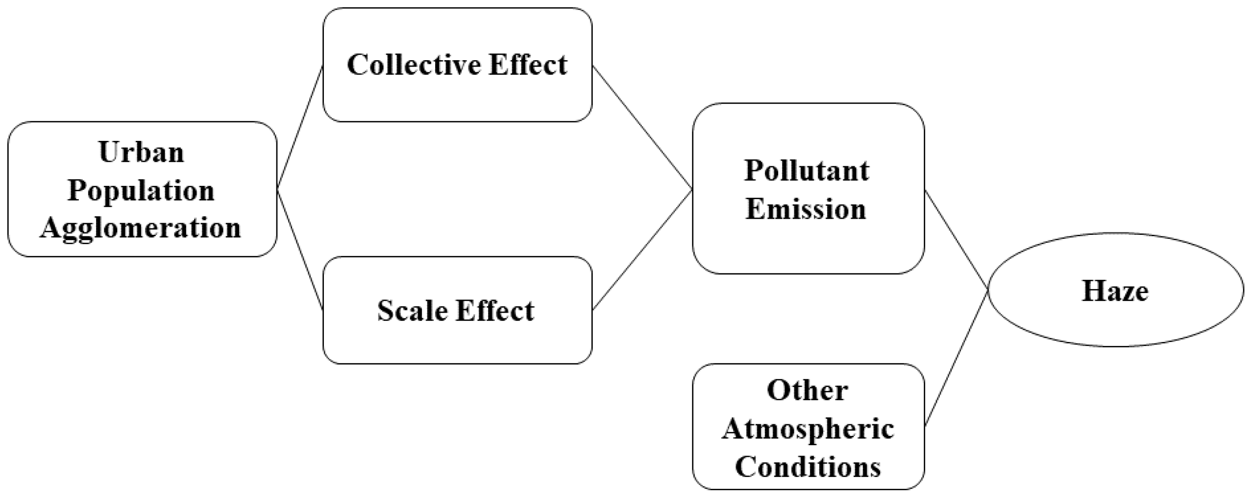
2.1. Analysis of Theoretical Mechanism

The action mechanism of urban population agglomeration on haze pollution is presently divided into two main views. The first is that population agglomeration will increase pollutant emissions in the atmosphere via the scale effect, making hazy weather more likely. According to some scholars [3,13], urban population agglomeration will cause traffic congestion, housing tensions, and high demand for heating and gas, which will generate a scale effect and increase pollutants in the atmosphere, resulting in haze pollution. On the contrary, another school of thought holds that increasing human density will lower pollution emissions in the atmosphere via the collective effect, aiding in the regulation of hazy weather. Although urban population agglomeration can cause a slew of issues, cities can serve the purpose of increasing resource efficiency. The agglomeration of a large number of people in cities allows them to take advantage of the city’s public transportation and pollution abatement infrastructure more fully, resulting in the collective effect and, as a result, a reduction in the emission of air pollutants, ultimately leading to a reduction in the haze pollution problem [14]. The reason why the two viewpoints indicated above reach different and opposing results is found in their development of two mesomeric effect models of urban population agglomeration on haze pollution: the scale effect and the collective effect, the routes of which are depicted in Figure 1.

2.1.1. Scale Effect

From the economic standpoint, the scale effect of urban population agglomeration on haze pollution is caused by externalities. The final consequence of combining the effects of each individual’s behavioral decisions is the influence of urban population agglomeration on haze pollution. According to a study conducted by Zeng Xiangang et al. [15], even though more than half of Beijing residents were aware of the severe health risks that haze would pose to themselves and their families, a sizable number of people were still unwilling to reduce the social health risks of haze in exchange for a lower quality of life and a higher cost of living. This study also shows that personal interests tend to take precedence over social interests in individual behavioral choices. As a result, as a city’s population proliferates, so do human activities and demands. At the same time, if people continue to think in terms of their interests and do not change their lifestyle habits, for example, in terms of travel, they will continue to drive motor vehicles, resulting in a large number of vehicle emissions due to an excess of motor vehicles and traffic congestion. This will have a scale effect on the haze pollution problem, with significant negative externalities for the urban environment.

2.1.2. Collective Effect

The formation of cities comprises population urbanization and two crucial features: non-agriculture industries and social modernization [16]. When a high population agglomeration leads to a city being formed, the collective effect becomes more significant. First, the spatial agglomeration of production activities in the urban industrial sector will lead production elements of various forms, accompanied by related industrial activities, to the city. As a result of these, the city’s allocable resources will be more plentiful. Second, as the urban industrial sector gradually improves its productivity, its public infrastructure will improve. At the same time, the city’s resource allocation will become more efficient. Finally, during urban development, distinct functional zones will be developed inside the city, depending on the location of the land, and there will be a concentration of similar activities within the same functional zone. Land intensification will increase, while social services will be improved. As a result, the urban collective effect to address the problem of air pollution prevention and control can efficiently deploy all types of plentiful resources and increase pollution prevention and control efficiency. For example, establishing a comprehensive public transportation and sewage system can strengthen pollutant treatment and prevention, establish a regional coordination management system, coordinate air pollution prevention and treatment, and ultimately reduce pollutant per capita emission to reduce haze pollution.

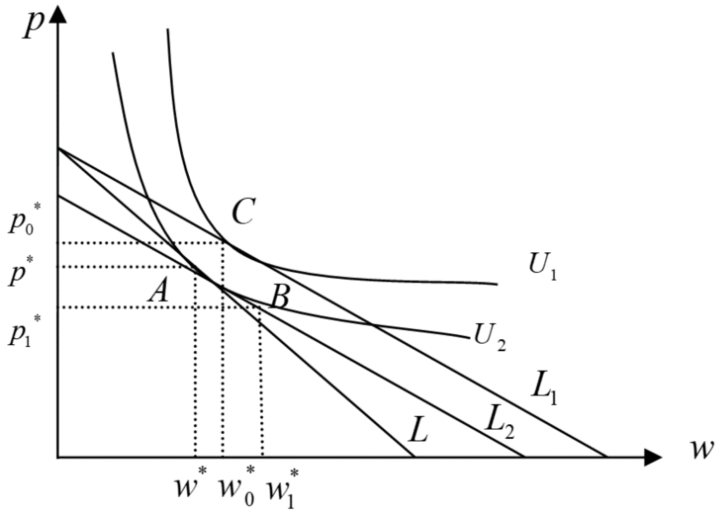
2.1.3. Reaction Mechanisms of the Two Effects

The two effects stated above result in two reaction mechanisms that influence haze pollution caused by urban population concentration. As indicated in Figure 2, w denotes haze concentration, and p denotes urban population density. Point A represents the equilibrium state attained with a haze concentration of w* and a population density of p* under the condition of urban environment carrying capacity U2. As population density rises, two mesomeric effects emerge—the scale effect and the collective effect. (1) If only the scale effect is taken into account, the increase in urban population density means more discharge of production and living pollutants. As shown in Figure 2, the combination line L of population density and haze concentration will be rotated to the right around its intersection with the vertical axis, giving rise to the line L1. If only the scale effect is taken into account, the environmental carrying capacity at U2 stays unaltered. Hence, the line L1 can be switched to L2 and intersect the environmental carrying capacity curve U2 at point B. At this time, the equilibrium point moves from the initial position A to B, and the haze concentration in the equilibrium state is w₁*. w₁* − w*, which is a positive value, represents the scale effect of population density increase, and it means that the scale effect will make the increase in urban population density lead to an increase in haze pollution concentration. (2) Consider the collective effect, which occurs as urban population density rises and people rush to the city. While people thoroughly enjoy the city’s socialized services, the city’s comprehensive public transportation system and pollution control and emission reduction system can reduce pollution generation. This is conducive to further strengthening the regulation and unified management of pollution caused by human activities. As a result, the city’s environment carrying capacity grows, and the curve U2 shifts to U1, intersecting with the combination line L1 of haze pollution and population density at point C. At this point, the equilibrium state of haze pollution concentration is w₀*. The haze concentration has decreased, based on w₁*. At this stage, the total effect of urban population density on haze pollution is w₀* − w*, indicating that an increase in urban population density eventually increases haze pollution concentration. (3) The scale effect and the intensification effect work together to produce a total effect, so when only the intensification effect is considered, the impact of the increase in population density on haze pollution can be obtained by subtracting the two, the result of which is w₀* − w₁*. It is a negative value, which suggests the scale effect makes the increase in urban population density reduce the concentration of haze pollution. Of course, Figure 2 only depicts one of the scenarios in which urban population agglomeration influences haze pollution due to the scale and collective combined effects. The direction and breadth of the influence of urban population agglomeration on haze pollution would also vary depending on the scale and collective effects. As a result, we suggest the following hypothesis:

H1: The correlation between urban population agglomeration and haze pollution may be non-linear.

H2: At this point, the impact of urban population agglomeration on haze pollution in China can be split into two mesomeric effects: the scale and the collective. The ultimate impact of human agglomeration on haze pollution is closely related to the dominant mesomeric effect.

2.2. Model Specification and Variable Description

2.2.1. Model Specification

Haze pollution is a meteorological issue caused by a combination of natural and human factors. Both its creation and dispersion are strongly impacted by atmospheric motion. The concentration of haze pollution in a region is equal to the haze produced in this region, minus the haze that spreads to other regions, plus the haze that spreads to this region from other regions. As a result, haze pollution seems to have a spatial correlation. If this spatial correlation is overlooked, it is impossible to adequately evaluate the relationship between other parameters such as urban population agglomeration and haze pollution, and the spatial spillover effect of haze itself cannot be accurately measured. As a result, a spatial econometric model is used for the analysis to make the estimation of the influence of urban population agglomeration on haze pollution more effective and accurate.

Due to the relative ease of the measuring course and the prominent economic connotation, the spatial lag model (SLM) and the spatial error model (SEM) have become two of the more basic and often employed models in spatial econometrics.

The following is the specific form of the spatial lag model:

$$y_{it}=\delta {{\displaystyle \sum }}_{j=1}^N{w}_{ij}{y}_{jt}+x_{it}\beta +u_i+{\phi }_t+{\epsilon }_{it}$$

(1)

In Equation (1), $w_{ij}$ is the element of the spatial weight matrix W, $u_i$ represents spatial fixed effects, ${\phi }_t$ represents time fixed effects, and ${\epsilon }_{it}$ represents the random error vector. $y_{it}$ represents the explained variable, and $x_{it}$ represents the primary explanatory variable and other control variables.

The following is the specific form of the spatial error model:

$$y_{it}=x_{it}\beta +u_i+{\phi }_t+{\nu }_{it}$$

(2)

$${\nu }_{it}=\lambda {{\displaystyle \sum }}_{j=1}^N{w}_{ij}{u}_{it}+{\epsilon }_{it}$$

(3)

The connotations in Equations (2) and (3) are nearly identical to those in Equation (1). On the other hand, the spatial error model acknowledges that other elements in the spatially related areas will have a spillover effect on the haze in the region.

The inverse distance principle is employed in this research to build the spatial weight matrix, which means that the reciprocal of the distance between two locations is used as the weight. The nearer the distance between the two places, the greater the weight; the further the distance, the lesser the weight. Furthermore, for simplicity of later measurement, the spatial weight matrix is frequently normalized by rows to equalize the influence of other spatial regions on the local region. However, to ensure that the mutual ratio between each element of the inverse distance spatial weight matrix remains unchanged and to maintain the weight matrix’s economic interpretation, this paper adopts an alternative weight matrix treatment proposed by Elhorst [17] and Kelejian et al. [18], i.e., each element of the inverse distance spatial weight matrix is divided by its largest eigenroot to obtain the normalized matrix.

2.2.2. Description of Primary Variables

First, in order to better control the influence of other factors on haze pollution so that the effect of population agglomeration on haze pollution will be measured more accurately, this study is based on the STIRPAT model widely used in the field of environmental economy. Select variables from four factors including environment, population, wealth, and technology are used to construct an empirical model of urban population agglomeration and smog pollution. The specific expression form of the STIRPAT model is shown in Equation (4):

$$I_{it}=a{P}_{it}^b{A}_{it}^c{T}_{it}^{d}e$$

(4)

In Equation (4), I is the environmental quality, P is the population, A is the per capita wealth, T is the technology, e is the error term, a is the model coefficient, and b, c, and d are the solve-for parameters. Equation (5) is produced by taking the logarithm of both sides of Equation (4):

$$\ln I_{it}=\ln a+b\ln P_{it}+c\ln A_{it}+d\ln T_{it}+\ln e$$

(5)

In this work, the relevant proxy variable will be used by the four key environmental factors in the STIRPAT model. Furthermore, in order to investigate the action mechanism of urban population agglomeration on haze pollution further—the scale effect and the collective effect—and to integrate various aspects of the relationship between urban population agglomeration and haze pollution, such as influence, representativeness, and data availability, we finally use the urban transportation sector as an example to assess and compare the influence of urban agglomeration on haze pollution. The bus ownership per 10,000 people was chosen as a proxy variable for the collective effect, and the occupying amount of civilian vehicles was chosen as a proxy variable for the scale effect.

Table 1. Description of Primary Variables.

Variables	Abbreviation	Connotation of the Variable	Average Value	Minimum Value	Maximum Value
Haze Concentration	Lnmean	Every 3 years’ moving average of PM2.5 concentration, and take the logarithm	3.7905	2.1031	4.6946
Population Density	Lndenpop	The average annual population of the municipal district divided by the built-up area, and take the logarithm	6.6746	2.5751	9.5453
Opening-Up Level	Lnfdi	The proportion of actual utilized foreign investment in local GDP in the municipal district, and take the logarithm	−4.1187	−8.8040	−0.8981
Economic Development Level	Lnrpgdp	After constant price treatment (base year–2001), the per capita GDP of the municipal district, and take the logarithm	9.9910	7.7630	12.1075
Industrial Structure	Lnindgdp	The proportion of secondary industry added value in local GDP in the municipal district, and take the logarithm	−0.6914	−1.8163	0.9517
Fixed-Asset Investment	Lnfasset	The total fixed-assets investment of the whole city (excluding farmers), and take the logarithm	14.0532	9.7746	17.9906
Scientific ResearchCapability	Lnsci	The proportion of scientific research employment in the total urban employment in the municipal district, and take the logarithm	−4.1422	−6.3652	−2.1148
Scientific ResearchInvestment	Lnexp_sci	The proportion of scientific research investment in local financial expenditure in the municipal district, and take the logarithm	−5.0789	−8.5620	−2.3067
Public Transportation	Lnbusp	The bus ownership per 10,000 people in the municipal district, and take the logarithm	1.6412	−1.1394	4.7074
Civilian Vehicles	Lnvehicle	The occupying amount of civilian vehicles of the whole city, and take the logarithm	11.6146	8.6995	15.3479

displays the relevant variable descriptions:

2.3. Data Sources

The explanatory variable in this paper, namely PM_2.5 concentration values, is obtained from the SEDAC. In 2012, China amended the Ambient Air Quality Standard (AAQS) (GB3095-2012) for the third time, revising the concentration limited values standard for some detecting indicators and increasing monitoring and reporting of PM_2.5 concentration limited values. The new AAQS was trialed in 74 prefecture-level cities across China in the same year. On 1 January 2016, the new AAQS was extended and applied across the country. Furthermore, the PM_2.5 statistics issued by China’s MEP are generated from ground detection stations, which are more accurate but cannot accurately quantify the average PM_2.5 concentration in a specific area. It is not possible to make a long-term assessment of the haze pollution condition in various regions of China based on PM_2.5 statistics published by China’s MEP in recent years. As a result, the PM_2.5 concentration data in this study are derived from the global annual average PM_2.5 surface concentration data given by SEDAC. Following the notion of Donkelaar et al. [19], the Battelle Memorial Institute (BMI) and Columbia University transformed the annual average PM_2.5 concentration data from aerosol concentration calculations using the relevant chemical model. Furthermore, the aerosol concentrations utilized for measurements are provided by satellite-mounted equipment, which improves the accuracy of the recorded data.

In terms of data processing, this research differs from other studies in that the variable of population density does not use the “population density” indicator published in the China Urban Statistical Yearbook for each prefecture-level city. The reason for this is that the “population density” indicator in the China Urban Statistical Yearbook is primarily calculated by dividing the gross population of the prefecture-level city at the end of the year by the administrative division area (including suburbs and some rural areas). This technique does not adequately reflect each prefecture-level city’s actual “urban population density.” As a result, the population density data in this study are calculated by dividing the annual average population of each prefecture-level city by the built-up area.

Other explanatory variables from CEInet Statistics Database and China City Statistics Yearbook (1999–2013) include the actual amount of foreign investment, per capita GDP, the proportion of secondary industry added value in the GDP, fixed-asset investment (excluding farmers), the bus ownership per 10,000 people, development land area, land area, scientific research employment, total urban employment, local financial expenditure, and local financial expenditure on scientific research. The civilian vehicles occupying amount is from China Statistical Yearbook for Regional Economic (2000–2013). The interpolation method was used to fill in the missing data that the above methods could not fill.

In summary, due to data availability constraints, the sample of 287 prefecture-level cities in China that underwent land withdrawal and city transformation after 1998 was deleted. After interpolation, the sample with an interpolation value less than 0 was removed, leaving a final sample of 2360 (236 × 10). Because the haze data were collected from a foreign-language website, the recording method was every three years’ moving average of the annual average PM_2.5 concentration values. Therefore, the data for the other variables were likewise taken as a three-year moving average. The time span of the overall sample includes 10 time units over the period 2001–2012.

2.4. Descriptive Analysis

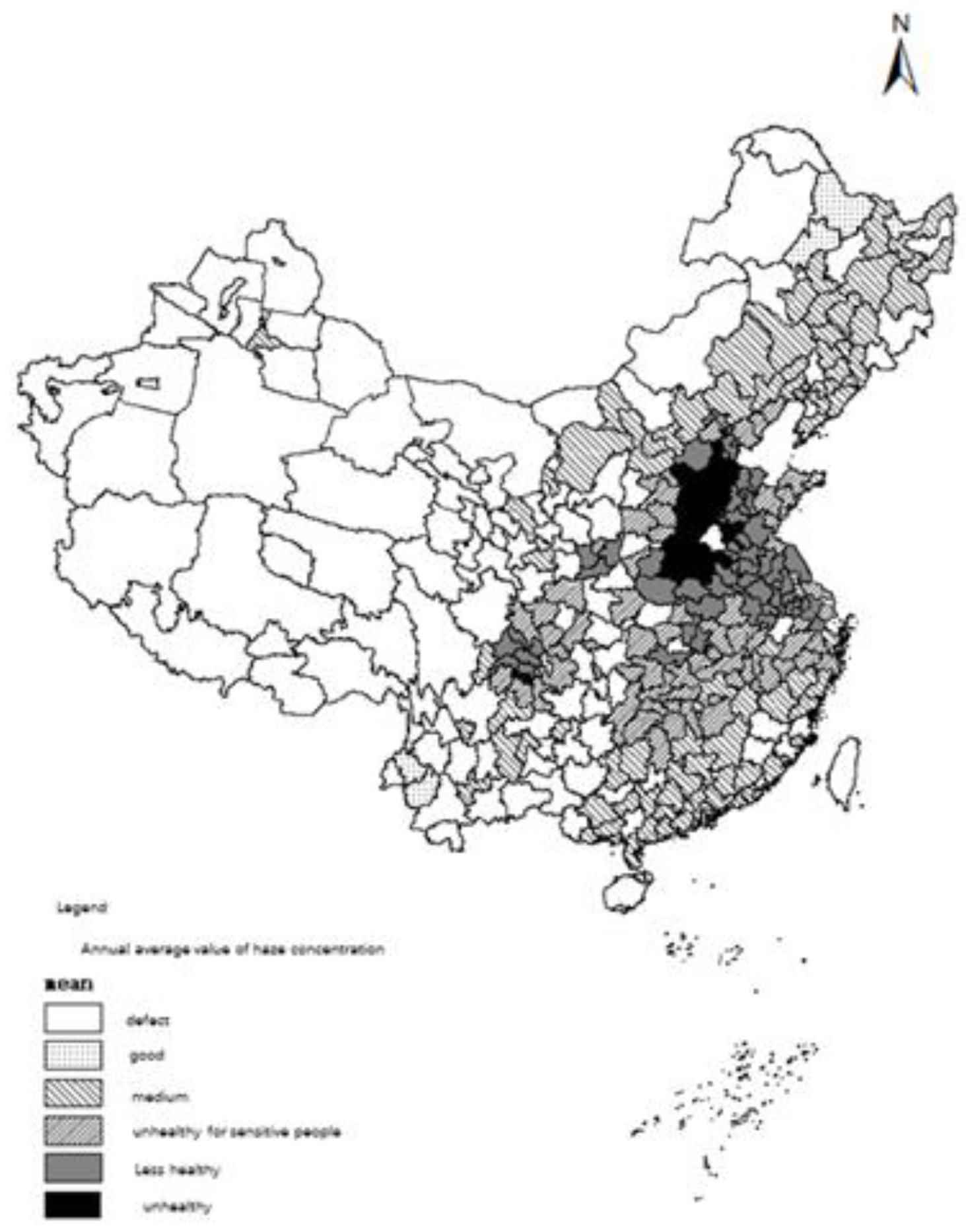
2.4.1. Analysis of the Current State of Urban Haze Pollution

The latest annual average PM_2.5 concentrations from 2010 to 2012 were plotted on a spatial distribution map (Figure 3) based on the annual average PM_2.5 data provided by Columbia University’s Socioeconomic Data and Applications Center (SEDAC), which are the data used for the empirical analysis in the following section as well.

As shown in Figure 3, areas that tend to be black represent the increasing severity of the haze pollution, and these areas are primarily located in the North China Plain and near the eastern coast of China. Furthermore, the annual average haze concentrations in the Sichuan Basin and Qinling Region area are higher, owing to the region’s topography, which is dominated by mountains and basins, and pollutants are not easily dispersed.

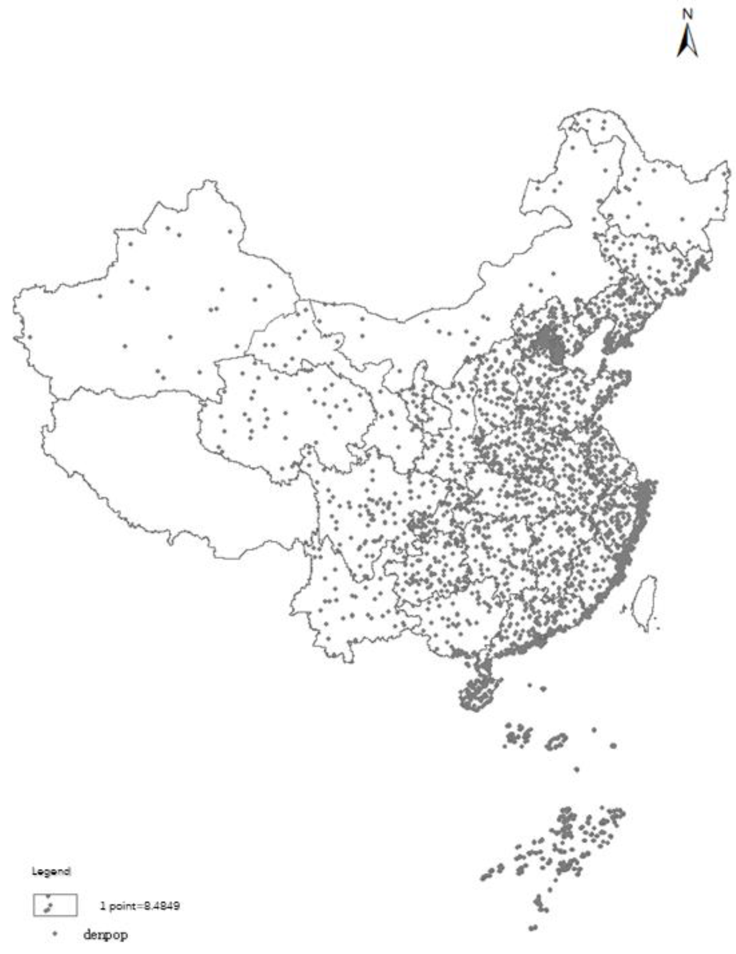
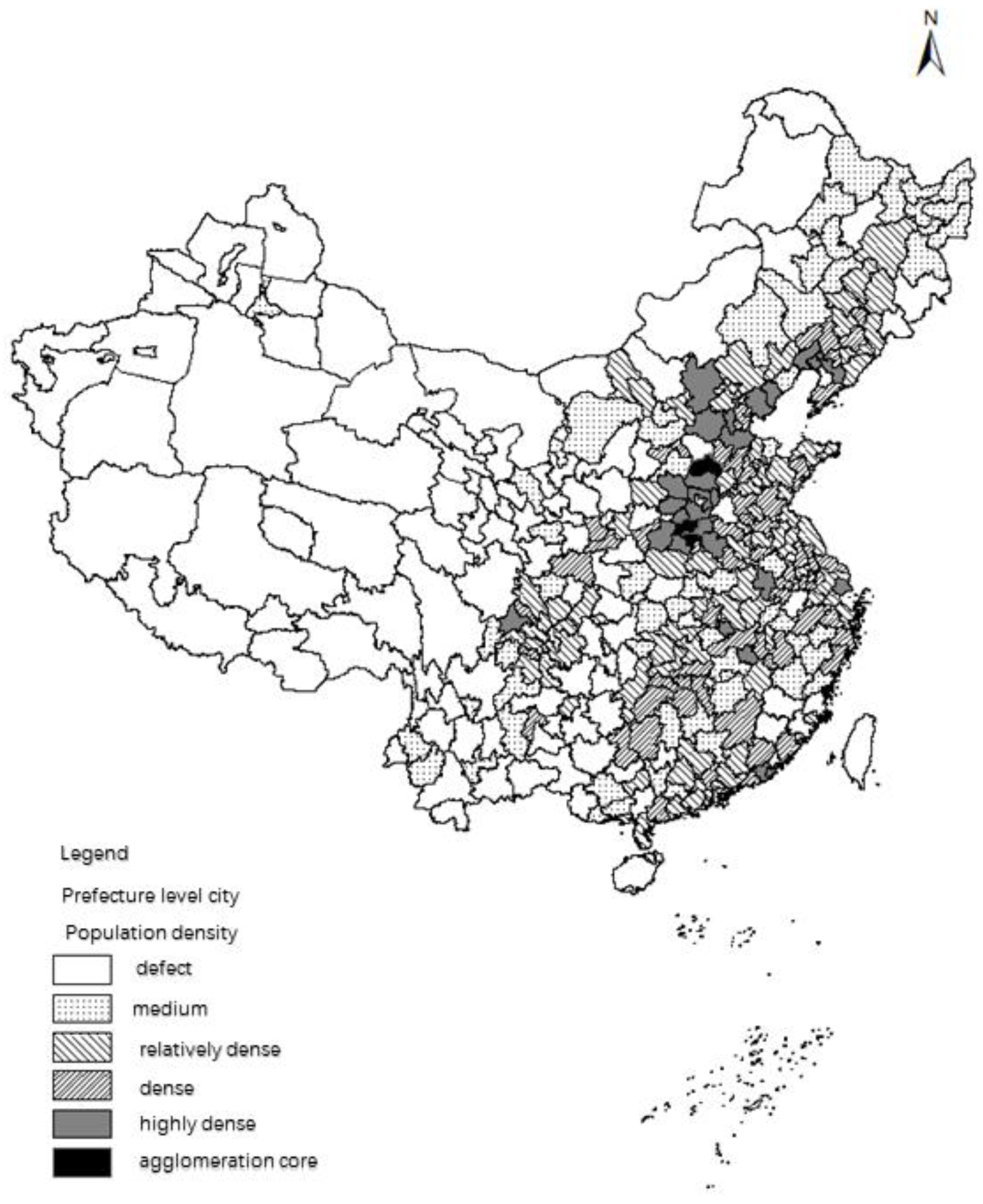
2.4.2. An Analysis of the Current State of Urban Population Density

The term “population density” refers to the population density data in China City Statistical Yearbook (2016). Because we focuse on urban population agglomeration, the term “population density” refers to the population density (per capita/km²) of municipal districts as reported in the China City Statistical Yearbook 2016. Figure 4 depicts China’s population density distribution map in conjunction with the country’s administrative map.

Figure 4 depicts China’s population distribution, marked by a dense population in the southeast and a sparse population in the northwest, with two unique distribution patterns along the Heihe–Tengchong line. China’s most densely populated places are the Beijing–Tianjin–Hebei region, the eastern coastal region, and the southeastern coastal areas. These regions contain three main Chinese city clusters: the Beijing–Tianjin–Hebei region, the Yangtze River Delta, and the Pearl River Delta. These locations are also primarily consistent with China’s higher levels of economic growth. Furthermore, Henan and Sichuan provinces have a high population density. These locations are relatively flat and resource-rich, making them ideal for human production and living activities.

To better compare with the annual average haze concentration in Figure 3, the population density data of each prefecture-level city from 2010 to 2012 were also taken as annual averages to generate the results shown in Figure 5. When comparing Figure 5 to Figure 3, it is clear that the regions with higher population density are also the regions with higher haze concentrations, which is especially evident in the Beijing–Tianjin–Hebei region, which is both an exceptionally densely populated region of China and a region with higher haze pollution levels. Furthermore, while some cities in the south are more densely populated than others, the number of populated cities in the north is higher overall. Figure 3 depicts the annual average haze concentration map, which shows that haze pollution is more severe in the north than in the south.

The following conclusions can be inferred from the descriptive statistics and empirical analyses shown above: (1) In China, the distribution of haze pollution is relatively concentrated. The North China Plain, the eastern coastal areas, and Xinjiang Uygur Autonomous Region are China’s most polluted hazy areas today. (2) China’s population distribution is characterized by a high density in the southeast and a low density in the northwest. The greater the region’s level of economic development, the greater the urban population agglomeration. Finally, a comparison of the regional distribution maps (Figure 3 and Figure 5) reveals that densely populated areas are essentially identical to areas with severe haze pollution. There is undoubtedly a spatial correlation between urban population density and haze concentration.

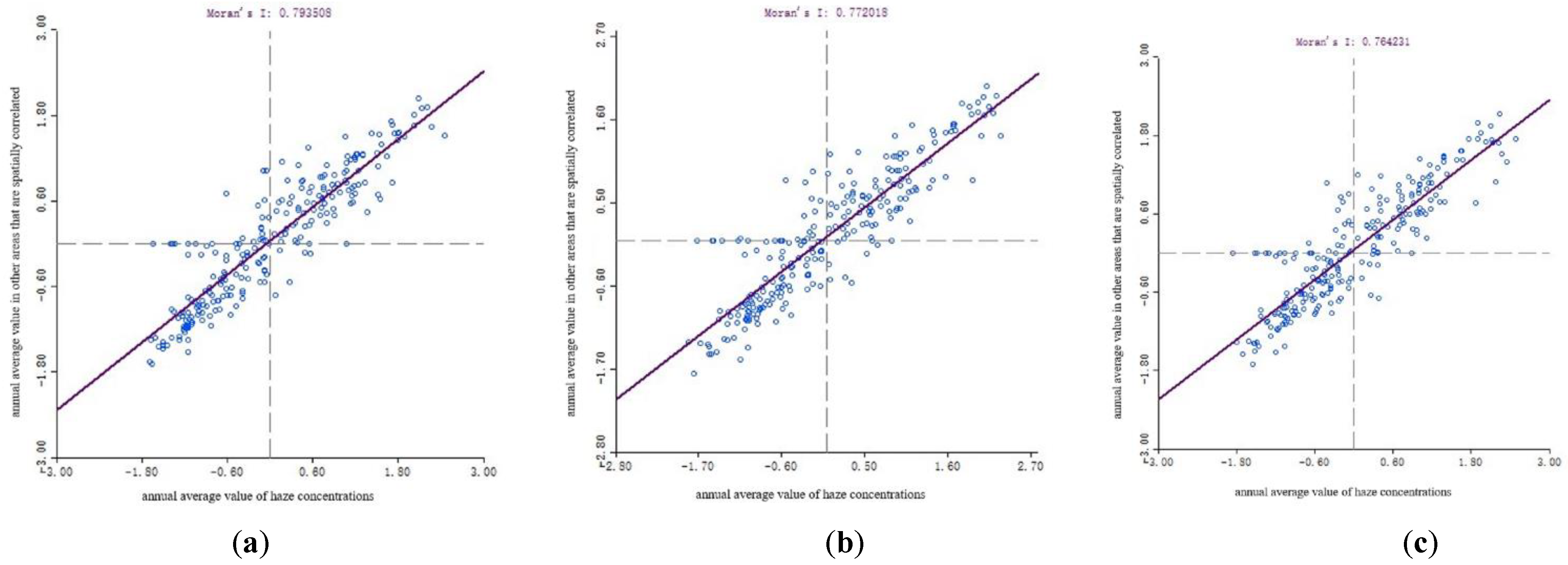
2.5. Testing of Spatial Panel Models

A necessary condition for the use of spatial econometric models is that the single variable or variables are spatially related and affect the validity of the estimated coefficients. We estimate a spatial correlation between haze pollution and population density based on the following description of the regional distribution of annual average PM_2.5 concentration values and urban population density in each prefecture-level city in China. However, the spatial relation should not be determined solely based on assumptions. Moran’s I index is used in this article to analyze the spatial relation for the core variable in this spatial panel data—the annual average PM_2.5 concentration values. PM_2.5 concentrations are moving averages taken for every three years due to data availability limits. This section chooses PM_2.5 concentration data for three sub-samples (2001–2003, 2005–2007, and 2010–2012) and depicts Moran’s I scatter plots, as seen in Figure 6:

Under the “chariot” contiguity principle, if two areas share a common boundary, they are considered proximate, and the index is set to 1. In contrast, if two areas do not have a common boundary, they are not proximate, and the index is set to 0. Based on the “chariot” contiguity principle, a spatial weight matrix of geographical proximity is built, and the global Moran’s I index of haze concentration is calculated. In academics, the global Moran’s I statistic is a widely used metric for assessing global spatial auto-correlation. According to the Moran’s I scatter plot of haze concentrations in Figure 6, the abscissa is the annual average value of haze concentrations during the representative year period. The ordinate is the annual average value of haze concentrations in other areas that are spatially correlated during the representative year period. Moran’s I indexes for the annual average value of haze concentrations in 2001, 2005, and 2010 are all bigger than 1. Furthermore, most of the scatter plot points are clustered in the first and third quadrants. These phenomena exhibit a spatial distribution of high-high and low-low clustering, reflecting the positive spatial correlation of haze pollution.

If a spatial autocorrelation exists, a suitable spatial econometric model must be chosen. This study uses the Lagrange multiplier test and a robust Lagrange multiplier test to pick a spatial lag model and a spatial error model based on the findings of the general panel model estimation. In addition, to determine the category of fixed effect in the spatial econometric model, a likelihood ratio (LR) test will be performed on the entity fixed effect and the temporal fixed effect.

Table 2. Moran’s I Index and Lagrange Multiplier Test Results.

Test Index	Mixed Effect	Spatial Fixed Effect	Temporal Fixed Effect	Two-Way Fixed Effects
LM-LAG	5465.49 ***	6412.10 ***	4380.32 ***	2008.70 ***
robust LM-LAG	811.51 ***	192.81 ***	654.34 ***	71.41 ***
LM-ERR	5662.97 ***	15,496.40 ***	4843.55 ***	1938.22 ***
robust LM-ERR	1008.98 ***	9277.11 ***	1117.57 ***	0.93
Moran I	0.25 ***	0.42 ***	0.23 ***	0.15 ***
LR Space	9337.32 ***
LR Time	1110.81 ***

Note: *** in the table represent the 1% significance levels, while LM-LAG and LM-ERR here refer to the chi-square value and p-value derived from the Lagrangian test for the absence of spatial lag and the LM test for the absence of spatial error, respectively.

displays the outcomes of the testing:

The test results for Moran’s I index are all greater than 0 for all four effects, as shown in Table 2, and pass the test at the 1% level of significance. These test results suggest that the data within the spatial scope examined in this research have a substantial positive spatial correlation. They also increase the persuasiveness of the spatial econometric model employed for the estimate in this paper. Regardless of whether the model employs fixed effects and what fixed effects are used, the combined likelihood ratio test results show that the spatial and temporal fixed effects pass the test at the 1% significance level. As a result, a two-way fixed-effects model with spatial and temporal fixed effects is preferable. The Lagrangian multiplier lag test, the Lagrangian multiplier error test, and the robust Lagrangian multiplier lag test all pass the significance test at the 1% level. However, the robust Lagrangian error test does not. Furthermore, when the Lagrangian multiplier lag test’s ${\mathit{\chi }}^2$ is compared to the Lagrangian multiplier error test’s ${\mathit{\chi }}^2$, the former is greater than the latter. When the robust Lagrangian multiplier lag test’s ${\mathit{\chi }}^2$ is compared to the robust Lagrangian multiplier error test’s ${\mathit{\chi }}^2$, the result is the same. As a result, the spatial lag model is preferable to the spatial error model for analyzing this spatial panel data.

3. Results and Discussions

Next, we will assess whether there is a non-linear relationship between urban population agglomeration and haze pollution as a whole. The spatial spillover effect of urban population agglomeration on haze pollution will also be assessed. We will then examine which of the two mechanisms of urban population agglomeration on haze pollution is dominant. Namely, the scale and collective effects provide some empirical reference for future policy formulation on urban population agglomeration and haze pollution control.

3.1. The Influence Effect of Urban Population Density on Haze Pollution

Based on the results of the Lagrange multiplier test and the likelihood ratio test described above, the spatial error model [1] and the spatial lag model results for two-way fixed effects were measured. However, the spatial lag model with two-way fixed effects is still the primary basis for future study. The results of the three spatial lag models estimated using spatial fixed effects, temporal fixed effects, and two-way fixed effects in space and time are shown in

Table 3. Spatial Lag Model Regression Results Under Three Fixed Effects. The first column is the variable name, and the last three rows represent the estimation results of the three spatial lag models under the variable space fixed effect, time fixed effect, and space and time double fixed effect.

Variable	Spatial Fixed Effect	Temporal Fixed Effect	Two-way Fixed Effect
Lnidenpop	1.3117 *** (2.6217)	−0.7101 *** (−2.8983)	1.3180 *** (2.6064)
Lnidenpop2	−0.1918 *** (−2.7357)	0.1584 *** (3.7865)	−0.1928 *** (−2.7215)
Lnidenpop3	0.0093 *** (2.8657)	−0.0088 *** (−3.7784)	0.0093 *** (2.8529)
Lnfdi	0.0002 (0.1203)	0.0141 ** (2.2996)	0.0000 (0.0009)
Lnrpgdp	−0.0013 (−0.1630)	−0.2492 *** (−14.9650)	0.0018 (0.2100)
Lnindgdp	0.0741 *** (5.6274)	0.2853 *** (8.8712)	0.0696 *** (5.1666)
Lnfasset	0.0084 ** (2.0860)	0.0915 *** (10.3035)	0.0116 ** (2.2569)
Lnsci	−0.0027 (−0.6482)	−0.0338 *** (−3.1389)	−0.0059 (−1.2067)
Lnexp_sci	−0.0060 *** (−2.6021)	0.0285 *** (2.7951)	−0.0076 *** (−2.6213)
${\delta }^2$	0.9650 *** (137.7361)	0.9870 *** (575.3820)	0.9826 *** (258.5835)
$R^2$	0.9907	0.6698	0.9907
${\sigma }^2$	0.0029	0.0914	0.0028

Note: *** and ** in the table represent 1% and 5% significance levels, respectively.

.

Table 3 indicates that the spatial spillover effects of haze pollution are all significantly positive and that urban population agglomeration has a considerable positive effect on haze pollution. ${\mathsf{\delta }}^2$ epresents the spillover effect of haze pollution, that is, the impact of local haze pollution on other spatially related areas. The two-way fixed effects spatial lag model, in particular, indicates that this spatial spillover effect leads to 0.9826. At the 1% significance level, it also passes the estimated coefficient test. This implies that haze pollution in the region will have a spillover effect on other spatially related areas and that the more severe the haze pollution in the region, the more severe the haze pollution in its neighboring areas.

As shown in Table 3, the results of the spatial lag model based on the two-way effect of spatial fixed and temporal fixed effects show that the population density’s absolute term, quadratic term, and cubic term all pass the estimated coefficient test at the 1% significance level. The absolute term, quadratic term, and cubic term coefficients are positive, negative, and positive, respectively. This concludes a significant non-linear relationship with an “N-shaped” curve between urban population agglomeration and haze pollution. According to current estimates, the inflection point values (persons/km²) are between 490 and 2053, and the impact of urban population agglomeration on haze pollution may be separated into three stages: First stage: The population density is relatively low to the left of the first inflection point value, and it essentially belongs to small and medium-sized cities in China. These cities have not invested sufficiently in constructing various public services and supporting facilities. The majority of small and medium-sized cities are experiencing accelerated urban economic development, with increased investment attraction and new factories. As a result, contaminants are difficult to treat efficiently, pollution sources are expected to persist unabated, and urbanization will likely worsen haze pollution. Second stage: Urban population agglomeration and haze pollution have an inverse connection between the two inflection points. This could be because the urban population has been reduced. Public infrastructure has been improved, so that the amount of pollution controlled and treated exceeds the amount of pollution emitted during urban development, resulting in a virtuous cycle between population agglomeration and the urban environment. Third stage: To the right of the second inflection point, the urban population agglomeration and haze pollution once again have a positive relation, but it differs from the first stage in that the city’s public facilities and services have been improved, but the city’s continued growth in population density has caused several problems. For example, in first-tier cities such as Beijing, Shanghai, and Shenzhen, the permanent population is significant, and the migrant population is massive, with core urban districts growing overcrowded and a high number of white collars commuting every day between the city center and the suburbs. The enormous permanent population has created a significant demand for housing and appliances in megacities, while longer commuting times have exacerbated traffic congestion and motor vehicle emissions. The total number of pollutants emitted is so large that the city’s self-regulatory function is “overloaded,” finally exceeding the carrying capacity of the urban environment and increasing the haze pollution problem.

In conclusion, there is an “N-shaped” association between urban agglomeration and haze pollution, and Hypothesis 1 is tested. So, are there two action mechanisms in this non-linear relationship between urbanization and haze pollution, and what are the magnitudes of the specific effects?

3.2. Tests of Two Effects of Urban Population Agglomeration on Haze Pollution

According to the above-mentioned theoretical mechanism analysis, the scale and collective effects are essential in the influence of urban population agglomeration on haze pollution. The empirical results of other socioeconomic parameters other than population density in Table 3 can validate this tentatively.

First, the city scale effect has a significant positive impact on haze pollution. (1) Both the secondary industry added value as a proportion of GDP and the amount of fixed-asset investment, which reflect the industrial structure of the city, have a significant positive effect on haze pollution, indicating that the city scale effect concentrates and increases a large number of industrial activities, contributing to the aggravation of the haze pollution problem. The most significant pollutants that contribute to haze pollution are toxic pollutants produced during industrial production. This analysis also reveals that some regions of China’s historic “three highs and one low” extensive growth model have contributed to haze pollution. (2) The majority of urban fixed-asset investment (excluding farmers) is spent on infrastructure and building investment, which reflects the degree of construction investment in the city to some extent. However, dust from construction sites is undeniably one of the major pollutants contributing to haze pollution. Too many construction projects, widespread renovations, and blind expansions can have a scale effect, aggravating haze pollution and potentially exacerbating the situation.

Second, the urban collective effect will exacerbate haze pollution. The urban agglomeration is usually accompanied by a cluster of additional talents, technology, and other elements that will help reduce haze pollution through knowledge spillover and technological innovation. As demonstrated in Table 3, the proportion of scientific research employment hurts haze pollution. However, it does not pass the significance level test. The amount of local fiscal investment in science and technology has a considerable detrimental impact on haze pollution. This finding suggests that, in combatting haze, the significance of the urban intensification effect should be fully recognized and that adequate government involvement and policy direction are also required. The proportion of science and technology expenditure in local financial expenditure has a considerable negative effect on haze pollution. This finding suggests that, in the process of combatting haze, the significance of the urban collective effect should be fully recognized, along with adequate government involvement and policy guidance. Increasing the percentage of science and technology expenditure in local financial expenditure will give more incentives for researchers to speed the transformation of research findings and develop strategies to eliminate haze. However, both of the above indicators are fairly tiny, which may be because technology’s contribution is mainly reflected in two areas: enhancing production efficiency and green emission reduction technology. The former focuses primarily on reducing industrial emissions through technological means; however, the lower the energy consumption, the lower the costs; thus, demand for industrial products increases rather than decreases, and total pollution emissions do not necessarily decrease. The latter focuses primarily on reducing industrial emissions and the treatment of pollutants emitted from industrial production, which plays a more direct role in pollution reduction. At the same time, this outcome is consistent with the reality that, at this level, technological factors play a minimal role in eliminating haze.

The preceding is preliminary proof of the opposite effect of scale and collective effects on haze pollution during the urban population agglomeration process. A more in-depth examination will follow. Which effect dominates in urban population agglomeration due to haze pollution? The final effect of urban agglomeration on haze pollution is connected to the outcome. It is impossible to describe all of the components involved in the scale and collective effects of urban agglomeration due to data availability constraints. As a result, this article seeks to analyze one of the main viewpoints—urban traffic—while also comparing the degrees of the scale and collective effects caused by urban population agglomeration. Based on actual monitoring data and component analysis, the literature [20,21] discovered that motor exhaust emissions, dust from construction sites, burning of crops such as straw, coal firing, and other secondary products are the primary sources of pollutants (or secondary aerosols) at this stage. This shows that the urban transportation sector was representative and significant for the study. The number of civilian vehicles owned by each prefecture-level city is chosen as a proxy variable for the scale effect in terms of variables’ setting. The bus ownership per 10,000 people in each prefecture-level city is chosen as a proxy variable for the collective effect. Both are mediators in the Sobel test for the effect of urban population agglomeration on haze pollution. This study assesses if the scale effect or the collective impact is substantial and whether the effect dominates at this stage.

Table 4. Mesomeric Effect of Urban Population Agglomeration on Haze. The first line is the name of the measured index, and the last two lines represent the results of the Sobel test when Bus Ownership per 10,000 people or Occupying Amount of Civil Vehicles are used as proxy or mediator variables, respectively.

Index	Bus Ownership per 10,000 people	Occupying Amount of Civil Vehicles
Sobel	−0.0063 *** (0.0018)	0.0123 *** (0.0029)
Goodman-1(Aroian)	−0.0063 *** (0.0018)	0.0123 *** (0.0029)
Goodman-2	−0.0063 *** (0.0018)	0.0123 *** (0.0029)
a coefficient	0.0926 *** (0.0139)	0.1859 *** (0.0167)
b coefficient	−0.0677 *** (0.0170)	0.0664 *** (0.0142)
Indirect effect	−0.0063 *** (0.0018)	0.0123 *** (0.0029)
Direct effect	0.2900 *** (0.0115)	0.2772 *** (0.0118)
Total effect	0.2837 *** (0.0115)	0.2896 *** (0.0115)
Mediation/total effct	−0.0221	0.0426
Indirect effect/direct effect	−0.0216	0.0445
Total effect/direct effect	0.9784	1.0445

Note: *** in the table denote 1% significance levels. Standard deviations are shown in parentheses.

displays the outcomes of the testing:

In general, the mediator’s influence is composed of two parts: the effect of the explanatory variable on the mediator (Path a) and the effect of the mediator on the explanatory variable (Path b). In addition, Path c₁ refers to the overall effect of the primary explanatory variable on the explanatory variable without taking the mediator into account. When the mediator is taken into account, Path c₂ refers to the effect of the primary explanatory variable on the explanatory variable. According to

Table 5. Direct, Indirect, and Total Effects of Different Factors on Haze Pollution.

	Effect	Direct Effect	Indirect Effect	Total Effect
Variable
Lndenpop		1.5923 ***	62.4951 **	64.0874 **
Lndenpop2		−0.2330 ***	−9.1437 **	−9.3767 **
Lndenpop3		0.0113 ***	0.4432 ***	0.4545 ***
Lnfdi		0.0000	−0.0007	−0.0007
Lnrpgdp		0.0022	0.0880	0.0903
Lnindgdp		0.0832 ***	3.2550 ***	3.3382 ***
Lnfasset		0.0141 **	0.5511 **	0.5652 **
Lnsci		−0.0070	−0.2727	−0.2797
Lnexp_sci		−0.0091 ***	−0.3554 **	−0.3644 **

Note: *** and ** in the table denote 1% and 5% significance levels, respectively.

, reviewing the specific paths in the mesomeric model reveals that the effect of Path c₂ is greater than Path c₁ when the bus ownership per 10,000 people is used as the mediator, indicating that encouraging the public to use public transportation and improving public infrastructure services are integral parts of the fight against haze pollution. However, when the occupying account of civilian vehicles is utilized as a mediator, the effect of Path c₂ is substantially smaller. The effect of the primary explanatory variable on the explanatory variable is much smaller than the total effect once the mediator is taken into account. The increased number of civilian vehicles will surely raise the emission of toxic gas in vehicle exhaust, “reinforcing” the beneficial effect of urban population agglomeration on haze pollution. As a result, Hypothesis 2’s prediction that two mesomeric mechanisms negatively impact haze pollution is substantially validated.

So, which of the two mesomeric effects of urban population agglomeration on haze pollution reigns supreme at this point? As shown in Table 5, the bus ownership per 10,000 people and the occupying amount of civilian vehicles in the city pass the mesomeric effect test at the 1% significance level. It also demonstrates that two action mechanisms significantly exist in the effect of urban agglomeration on haze pollution. When the bus ownership per 10,000 persons in the city is used as the mediator, the indirect effect is −0.0063, and the proportion of this mesomeric effect in the total effect is −0.0221. When the occupying amount of civilian vehicles is utilized as the mediator, the indirect effect is 0.0123. The proportion of this mesomeric effect in the total effect is 0.0426. A comparison demonstrates that the mesomeric effect in the first situation contributes much less to the total effect than it does in the second situation. The “collective effect,” indicated by the bus ownership per 10,000 persons in the city, is far less than the “scale effect,” expressed by the occupying amount of civilian vehicles. This demonstrates that, at this time, the scale effect outweighs the effect of population agglomeration on haze pollution. The findings of this empirical study are also typically congruent with reality. With a significant number of people congregating in China’s first- and second-tier cities, the demand for transportation, housing, and life has skyrocketed. However, many creative technology achievements have not been rapidly transformed and adapted to urban life, and people’s consuming habits and attitudes have not significantly altered. Although first-tier cities such as Beijing and Shanghai have long used traffic restrictions and a lottery for license plates to govern urban traffic, the number of individuals buying vehicles and playing the lottery is increasing; despite repeated national attempts to regulate and control housing prices, real estate developers around the country are developing new construction in significant numbers. On the contrary, due to technical progress not being fully mature, relative discomfort, and consumer attitudes, new energy cars and electric vehicles have not been widely marketed and used. As a result, to tackle the problem of haze pollution, we might try to consider and design policies to suppress the scale effect caused by urban population agglomeration and improve the collective effect.

3.3. Subdivision of the Effect of Urban Population Agglomeration on Haze Pollution

The degree of various socioeconomic factors’ effects on haze pollution is direct and indirect. A difference will be drawn here between direct and indirect effects. Direct effects refer to the direct action of changes in regional socioeconomic variables, while indirect effects are the spatial spillover effects of changes in regional socioeconomic variables. The estimated direct effects, indirect effects, and total effects of the explanatory variables on the core variables are shown in Table 5. The results suggest that population agglomeration has a significant positive effect on haze pollution, both directly and indirectly, which is consistent with our prior findings. Other factors’ effects on haze pollution’s direct and indirect effects remain essentially consistent. Population density, the proportion of secondary industry added value in GDP, fixed-asset investment (excluding farmers), and the proportion of scientific research expenditure in local governmental expenditure pass the coefficient tests with varying degrees of significance. It is also worth mentioning that the indirect effect of all socioeconomic factors on haze pollution is substantially more significant than the direct effect, demonstrating that haze pollution is vulnerable to the interaction of socioeconomic factors across regions.

4. Conclusions

4.1. Conclusions

Based on the preceding analysis, the paper’s conclusions are: (1) Positive spatial correlation is a characteristic of haze pollution. Haze pollution in the region will be influenced by natural and artificial variables such as atmospheric movements and industrial transfers, affecting locations geographically proximate to the region. Similarly, air pollution in other places will impact urban air quality in the region. (2) There is a significant “N-shaped” non-linear relationship between urban population agglomeration and haze pollution. This suggests that, allowing for other socioeconomic factors, as urban population density increases, haze pollution tends to increase, then drop, then increase again. The reason for this is that at different levels of urban population agglomeration, the intensity and efficiency (the collective effect) of investment in public infrastructure and services and demand (the scale effect) for housing, home appliances, and motor vehicles fluctuate. (3) In China, the scale effect of urban population agglomeration on haze pollution is currently more significant than the collective effect. Most Chinese cities are still in the “accelerated development stage,” with the rate of population urbanization significantly outpacing the rate of social service urbanization. Because urban infrastructure such as public transportation, health care, and education are still in the early stages of investment and construction, cities cannot exploit the benefits of efficient resource allocation fully, nor can they “regulate” and “alleviate” urban environmental issues. (4) The scale and collective effects negatively impact haze pollution, as evidenced by disparities in the impact of associated socioeconomic factors. The proportion of secondary industry added value in GDP and the urban fixed-asset investment have a significant positive effect on haze pollution in the region and a significant positive spatial spillover effect on spatially related areas. Meanwhile, local government investment in scientific research has a considerable impact on haze pollution prevention and control and a negative spatial spillover effect on haze pollution. (5) The indirect effect (or spatial spillover effect) of urban population agglomeration on haze pollution is much more significant than the direct effect. The same can be said about the effects of other socioeconomic factors on haze pollution. This demonstrates that other socioeconomic factors in spatially related areas are more likely to influence local haze pollution than local socioeconomic factors.

4.2. Policy Implications

(1) Effective haze pollution prevention and management necessitates completely using the collective effect induced by urban population agglomeration and successfully controlling the scale effect caused by it. Specifically:

(2) City layouts should be scientifically designed, and the size of the urban population should be reasonably regulated. The aims of city regulation should include transferring some of the urban functions of super-large and large cities, improving the social and economic development of small and medium-sized cities, attracting people to move to them, and so on. Simultaneously, a city should increase its investment in the development in urban pollution control and emission reduction systems as well as improvements to public infrastructure. Governments at all levels should tighten their control over the approval criteria for urban fixed-asset investment projects while streamlining the approval process and severely controlling duplication of urban construction projects. Governments should also manage to increase active public engagement, stimulate the use of public transportation, and improve resource use efficiency. They should create a sound urban management system to assist city inhabitants in developing green travel habits by providing subsidies, fines, and traffic restrictions.

(3) Regional cooperation should be strengthened to coordinate policies on haze prevention and control. Joint prevention and control is a necessary way to combat haze. Each region could not avoid haze pollution itself but chose to strengthen communication and cooperation in order to complete a systematic regional coordination mechanism for atmospheric pollution prevention and control sooner. The keys to controlling haze pollution include modifying urban industrial structures, restricting high energy-consuming enterprises, and improving emission reduction and pollution control technologies.

(4) It is important to increase production efficiency, encourage green development and increase source and process management. We will raise awareness of “green production” and “green consumption” on both the supply and demand through policy advice and political assistance. We will strengthen the power of innovation and research in energy conservation and emission reduction and the ability to transform scientific and technological achievements, raise environmental awareness among manufacturing enterprises and the general public, and bring the market’s role in regulating urban production and lifestyle into play.

References

1. Guan, D.; Su, X.; Zhang, Q.; Peters, G.P.; Liu, Z.; Lei, Y.; He, K. The Socioeconomic Drivers of China’s Primary PM2.5 Emissions. Environ. Res. Lett. 2014, 9, 1–9. [Google Scholar] [CrossRef] [Green Version]
2. Ma, L.M.; Zhang, X. The Spatial Effect of China’s Haze Pollution and the Impact from Economic Change and Energy Structure. China Ind. Econ. 2014, 4, 19–30. [Google Scholar]
3. Shuai, S.; Xin, L.; Cao, J.; Yang, L. China’s Economic Policy Options for Governing Fog Pollution—Based on the Perspective of Spatial Spillover Effect. Econ. Res. J. 2016, 9, 73–88. [Google Scholar]
4. Leng, Y.; Du, S.Z. Energy price distortion and haze pollution: The Evidence from China. Ind. Econ. Res. 2016, 1, 71–79. [Google Scholar]
5. Shoufeng, H. Environmental regulation, shadow economy and smog pollution. Econ. Perspect. 2016, 11, 33–44. [Google Scholar]
6. Quan, S.W.; Huang, B. Embedding Effects in Evaluation of Multiple Environmental Policies—Evidences from Beijing’s Haze and Sand Control Policies. China Ind. Econ. 2016, 8, 23–39. [Google Scholar]
7. Zhang, X.Y.; Wang, Y.Q.; Lin, W.L.; Zhang, Y.M.; Zhang, X.C.; Gong, S.; Zhao, P.; Yang, Y.Q.; Wang, J.Z.; Hou, Q.; et al. Changes of atmospheric composition and optical properties over Beijing—2008 Olympics monitoring campaign. Bull. Am. Meteorol. Soc. 2009, 90, 1633–1651. [Google Scholar] [CrossRef] [Green Version]
8. Shi, Q.L.; Guo, F.; Chen, S.Y. “Political Blue Sky” in Fog and Haze Governance—Evidence from the Local Annual “Two Sessions” in China. China Ind. Econ. 2016, 5, 40–56. [Google Scholar]
9. Zhang, S.L.; Li, Y. Different Government Smog Governance Strategies in Response to Public Opinion. Comp. Econ. Soc. Syst. 2016, 3, 52–60. [Google Scholar]
10. Chen, S.Y.; Chen, D.K. Energy Structure, Haze Governance and Sustainable Growth. J. Environ. Econ. 2016, 1, 59–75. [Google Scholar]
11. Ma, L.M.; Liu, S.L.; Zhang, X. Study on Haze Pollution Induced by Energy Structure and Transportation: Based on Spatial Econometric Model Analysis. Finance Trade Econ. 2016, 1, 147–160. [Google Scholar]
12. Xiang, K.; Song, D.Y. Spatial Analysis of China’s PM2.5 Pollution at the Provincial Level. China Popul. Resour. Environ. 2015, 25, 153–159. [Google Scholar]
13. Qin, M.; Liu, X.Y.; Tong, Y.T. Does Urban Sprawl Exacerbate Haze Pollution—An Empirical Study of Fine Particles(PM2.5) in Chinese Cities. Finance Trade Econ. 2016, 11, 146–160. [Google Scholar]
14. Glaeser, E. Triumph of the City: How Our Greatest Invention Makes Us Richer, Smarter, Greener, Healthier, and Happier; Runquan, L., Translator; Shanghai Social Sciences Press: Shanghai, China, 2012; pp. 113–131. [Google Scholar]
15. Zeng, X.G.; Xie, F.; Zong, Q. Behavior Selection and Willingness to Pay of Reducing PM2.5 Health Risk: Taking Residents in Beijing as an Example. China Popul. Resour. Environ. 2015, 25, 127–133. [Google Scholar]
16. Chun, L. On China’s Urbanization: Knowledge Rebuilding and Practice Rethinking. Popul. Res. 2013, 37, 3–15. [Google Scholar]
17. Elhorst, J.P. Dynamic Models in Space and Time. Geogr. Anal. 2001, 33, 119–140. [Google Scholar] [CrossRef] [Green Version]
18. Kelejian, H.H.; Robinson, D.P. Spatial Correlation: A Suggested Alternative to the Autoregressive Model—New Directions in Spatial Econometrics; Springer: Berlin/Heidelberg, Germany, 1995; pp. 75–95. [Google Scholar]
19. Donkelaar, A.; Martin, R.V.; Brauer, M.; Kahn, R.; Levy, R.; Verduzco, C.; Villeneuve, P.J. Global Estimates of Exposure to Fine Particulate Matter Concentrations from Satellite-based Aerosol Optical Depth. Environ. Health Perspect. 2010, 118, 847–855. [Google Scholar] [CrossRef] [PubMed] [Green Version]
20. Lv, B.L.; Zhang, B.; Bai, Y.Q. A systematic analysis of PM2.5 in Beijing and its sources from 2000 to 2012. Atmos. Environ. 2016, 124, 98–108. [Google Scholar] [CrossRef]
21. Li, X.Y. Empirical Analysis of the Smog Factors in Beijing-Tianjin-Hebei Region. Ecol. Econ. 2016, 32, 144–150. [Google Scholar]
Figure 1. Schematic Diagram of Two Action Mechanisms of Urban Population Agglomeration on Haze Pollution.
Atmosphere 13 00278 g001
Figure 2. Schematic Diagram of the Reaction Mechanisms of Urban Population Agglomeration Affecting Haze Pollution. w denotes haze concentration, and p denotes urban population density. Line L is a combination of population density and haze concentration. Curve U represents environmental carrying capacity. Point A represents the equilibrium state attained with a haze concentration of w* and a population density of p* under the condition of urban environment carrying capacity U2.
Atmosphere 13 00278 g002
Figure 3. Annual Average Concentration of Haze from 2010 to 2012 in Chinese Prefecture-Level Cities. Source: Map of Global Annual Average Surface PM2.5 Concentrations from SEDAC. https://sedac.ciesin.columbia.edu/ (accessed on 20 December 2021).
Atmosphere 13 00278 g003
Figure 4. Spatial Distribution Map of Point Density in Chinese Population Density in 2015.Data Source: China City Statistical Yearbook 2016. https://www.tongjinianjian.com/111090.html (accessed on 20 December 2021).
Atmosphere 13 00278 g004
Figure 5. Annual Average Population Density Map of Chinese Prefecture-Level Cities during 2010–2012. Data Source: China City Statistical Yearbook (2012–2013). https://www.tongjinianjian.com/111090.html (accessed on 20 December 2021).
Atmosphere 13 00278 g005
Figure 6. Scatter Plots of PM2.5 in Prefecture-Level Cities in Some Years under the Geographical Proximity Weight Matrix. Source: Satellite Map of Global Annual Average Surface PM2.5 Concentrations From SEDAC. The diagonal lines mean trend line of these scatter points. (a) Moran’s I scatter plot of PM2.5 concentration values from 2001 to 2003. (b) Moran’s I scatter plot of PM2.5 concentration values from 2005 to 2007. (c) Moran’s I scatter plot of PM2.5 concentration values from 2010 to 2012.
Atmosphere 13 00278 g006