1. Introduction
Atmospheric dispersion models are common in the field of environmental science and are usually applied to simulate large-area and long-term pollutant emissions. With the increasing demand for emergency response, they have been used to simulate sudden leakage of harmful gases as well. However, traditional atmospheric dispersion model programs feature serial execution. The existing parallelization methods are not completely applicable to emergency simulation cases. Certain cases require high temporal and spatial resolution, which results in a high computation load. In such cases, the programs suffer from long execution time. For example, it takes about 70 s for the CALPUFF model to simulate a case with 1600 computational grid cells and 480 time steps. When the number of grid cells increases to 160,000, the simulation takes about 800 s. It is difficult for simulation to meet the need for results to be obtained as soon as possible for emergency response. Therefore, it is critical to parallelize the atmospheric dispersion models.
Recently, many scholars have exploited parallel computing interfaces such as MPI (Message Passing Interface) and CUDA (Compute Unified Device Architecture) to optimize the source code of the atmospheric dispersion model to achieve parallelization. For example, Kleeman et al. used MPI to accelerate the CALPUFF model [
1]. Pinheiro et al. used CUDA to accelerate the radionuclide dispersion model [
2], and Cremades et al. used CUDA to accelerate the CALPUFF model [
3]. These methods all require profiling to find the most time-consuming function in the program for optimization, focusing on accelerating the module where the function is located. For the CALPUFF model system, they are usually suitable for the dispersion module, and not applicable to the wind field module.
At the same time, scholars have proposed several methods to directly divide the pollution sources, receptors, and simulation periods in the computation task without changing the source code. For example, Yao et al. and Hu et al. both accelerated the Gaussian model by dividing multiple pollution sources in the experimental cases [
4,
5]. Yau et al. accelerated the CALPUFF model by dividing multiple pollution sources and types of pollutants in the experimental cases [
6]. Canada’s Lakes Environmental Company developed the commercial software CALPUFF View and implemented parallel computation for the CALPUFF model by dividing the simulation period. While these methods are convenient and easy to implement, they are not applicable to cases without those features.
Compared with the simple Gaussian model, the CALPUFF model can calculate the three-dimensional wind field and has higher accuracy. Meanwhile, the CALPUFF model has a higher calculation speed than the complex numerical simulation method. These advantages make the CALPUFF model more suitable for the emergency field [
7]. In emergency cases, there is often only one pollution source, and the simulation period is relatively short. This paper proposes a method for dividing the computation tasks for the CALPUFF model with multiple layers of receptors and conducts a performance test on the cloud platform.
2. Methods
2.1. Basic Theory of Atmospheric Dispersion Model
The atmospheric dispersion model explores the processes of the dispersion, transportation, transformation, and deposition of pollutants in the atmosphere. Thus, it is widely used for environmental assessment and emergency response. In theory, the atmospheric dispersion model can be divided into three categories: Gaussian models, Lagrangian models, and Eulerian models. Gaussian models simulate pollutants based on the Gaussian plume distribution formula. This model has the highest computation speed and lowest accuracy. Lagrangian models divide pollutants into smaller units and calculate their trajectories separately, then integrate them. These can be further divided into trajectory models and puff models. Specifically, trajectory models divide pollutants at the particle level, while puff models divide them into “puffs” with a certain volume, then uses the Gaussian method within the puffs. This type of model improves simulation accuracy while maintaining a relatively high computation speed. Eulerian models use numerical simulation methods to solve the partial differential equations of mass conservation in the atmosphere [
8]. They have the lowest computation speed and highest accuracy. A comparison of the three models is presented in
Table 1, and the Lagrangian puff model CALPUFF is chosen for our further research.
2.2. Introduction of CALPUFF Model System
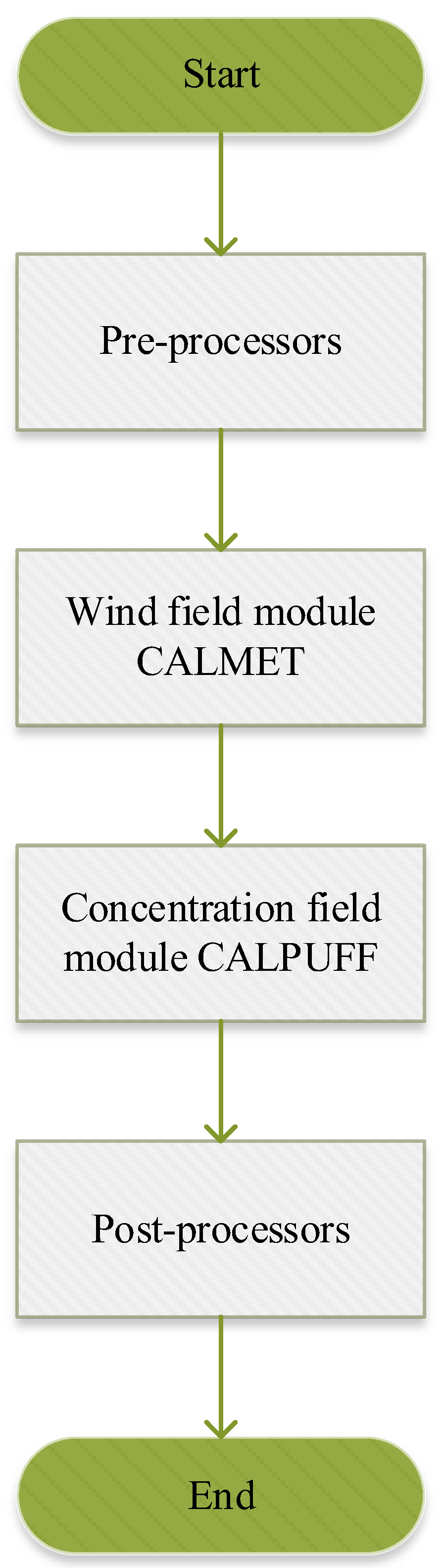
The CALPUFF model is a diagnostic wind field model developed by Sigma Research Corporation and approved by the US Environmental Protection Agency. The CALPUFF model system consists of the meteorological model CALMET, dispersion model CALPUFF, and a number of pre-processors and post-processors [
9]. Taking terrain elevation data, land use data, and meteorological observation data as input, the CALMET module generates a three-dimensional wind field. Taking the wind field and pollution source information as input, the CALPUFF module generates a three-dimensional concentration field. The CALPUFF model is a Lagrangian puff model that treats the pollution as a superposition of several “puffs” with a certain volume. It calculates the Lagrangian trajectory for these puffs and uses the Gaussian method inside each puff. The flow of the CALPUFF model is illustrated in
Figure 1.
2.3. Parallelization Method
In a large-scale atmospheric dispersion simulation, there are usually multiple independent objects of the same type (such as multiple pollution sources, etc.), which is the key of parallelization. These objects can be assigned to different computing nodes for parallel computation, then the results can be merged. The two main time-consuming modules of the CALPUFF model are the CALMET module for wind field calculation and the CALPUFF module for concentration field calculation. These two modules require different methods for parallelization.
2.3.1. Parallelization Method for the CALMET Module
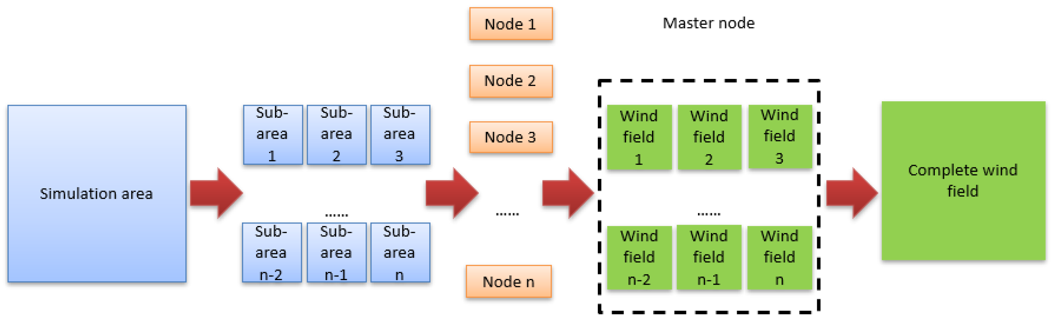
The CALMET module is irrelevant to pollution sources and receptors. Existing parallelization methods usually divide the simulation period, i.e., temporal division. However, existing methods cannot be applied to cases where the simulation period is less than one day, as CALMET considers daily changes in the atmosphere and requires that the start time of a simulation must be earlier than 5 a.m. in the local time. Because the simulation period in many emergency cases is less than one day, the method of dividing the simulation area (i.e., spatial division) is adopted in this study in order to improve its applicability to emergency cases.
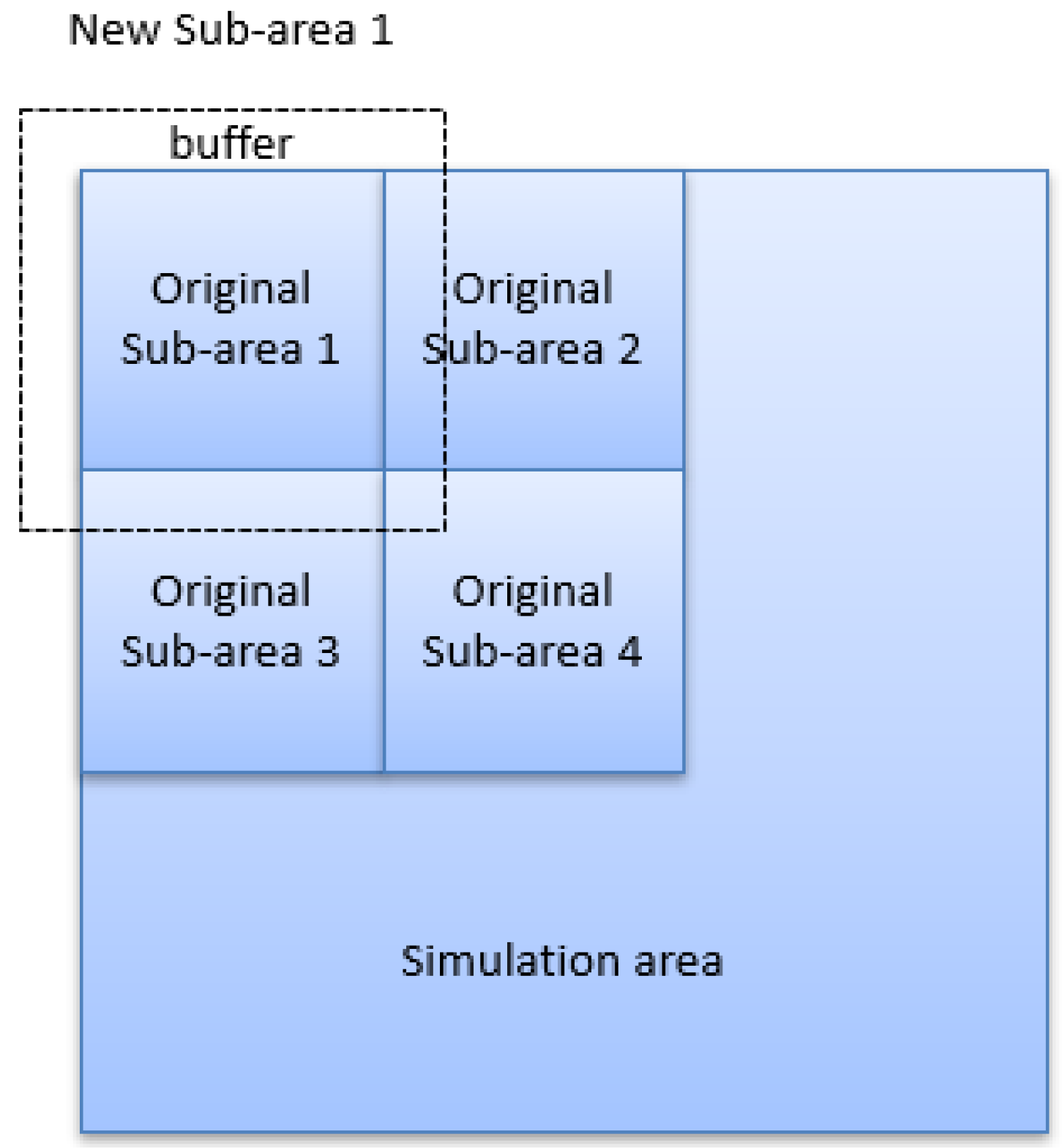
The diagnostic wind field is based on mass conservation and boundary conditions, and the values of the boundary cells are not reliable. Therefore, buffer zones should be added to the sub-areas. In addition, the errors formed by square division are smaller than with rectangular division, because the boundary length of a square is smaller than that of rectangles with the same area [
10]. The division method is illustrated in
Figure 2.
As shown in
Figure 3, the buffer method means that the range of each sub-area is expanded to ensure the reliability of the values of the cells on the original boundary. The southwest corner coordinates of the new sub-area and numbers of rows and columns are input to the module. When merging files, the values of the buffer cells are abandoned.
After receiving the calculation request, the master node divides the simulation area into several parts equally along the x and y axes and sends the coordinates of these sub-areas with buffers to each computing node. Then, the computing nodes run the CALMET module on the corresponding sub-areas and send the results back to the master node. Finally, the master node merges the resulting files to obtain the complete wind field.
2.3.2. Parallelization Method for the CALPUFF Module
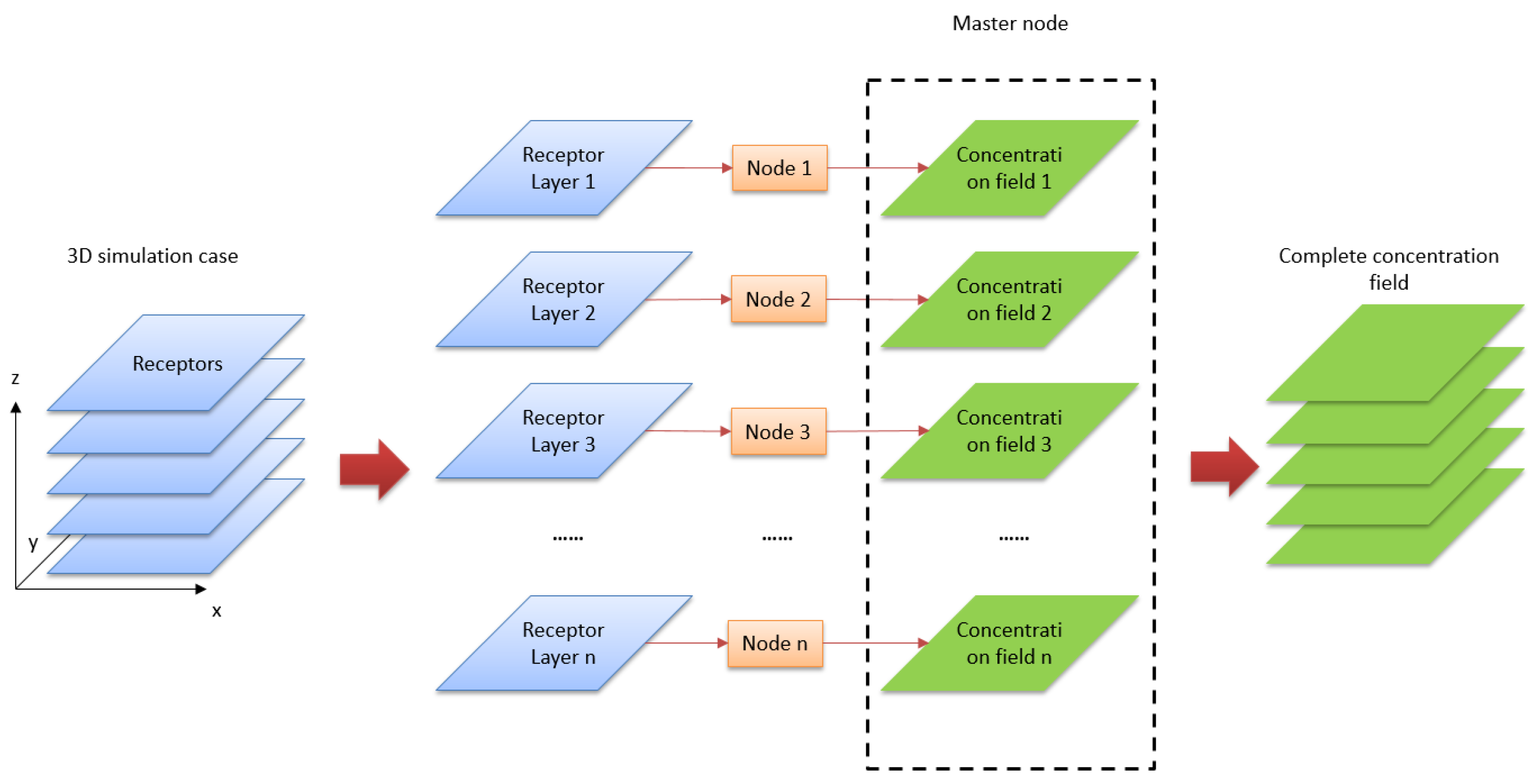
Due to the characteristics of the Lagrangian puff model, the simulation process in the CALPUFF module is continuous and difficult to parallelize. However, there are parallelization opportunities for certain specific cases. Currently, the CALPUFF module is mainly used for ground concentration calculation, and the calculation of a three-dimensional concentration field is relatively rare. In fact, CALPUFF can output a three-dimensional concentration field, which is significant for emergency response. In a three-dimensional simulation case, there are usually multiple layers of receptors along the
z-axis, which can be calculated in parallel on the computing nodes, as illustrated in
Figure 4.
After receiving the calculation request, the master node assigns the complete wind field file and the information of the layers to each computing node. Then, the computing node runs the module on one layer and sends the results back to the master node. Finally, the master node integrates the resulting files to obtain the complete concentration field.
For this module, the existing parallelization method usually divides the pollution sources in a multi-source environmental simulation case. By contrast, a parallelization method is provided in this paper for many emergency simulation cases with only one pollution source.
2.3.3. Parallel Algorithm Flow
As mentioned in Hu 2010, MPI is mostly used for communication between nodes in complex parallel computing, while a lightweight middleware or self-programming could be applied in simple parallel computing. RabbitMQ is an open-source implementation of the message queue which provides the function of communication and task scheduling. Therefore, we chose RabbitMQ as a communication middleware.
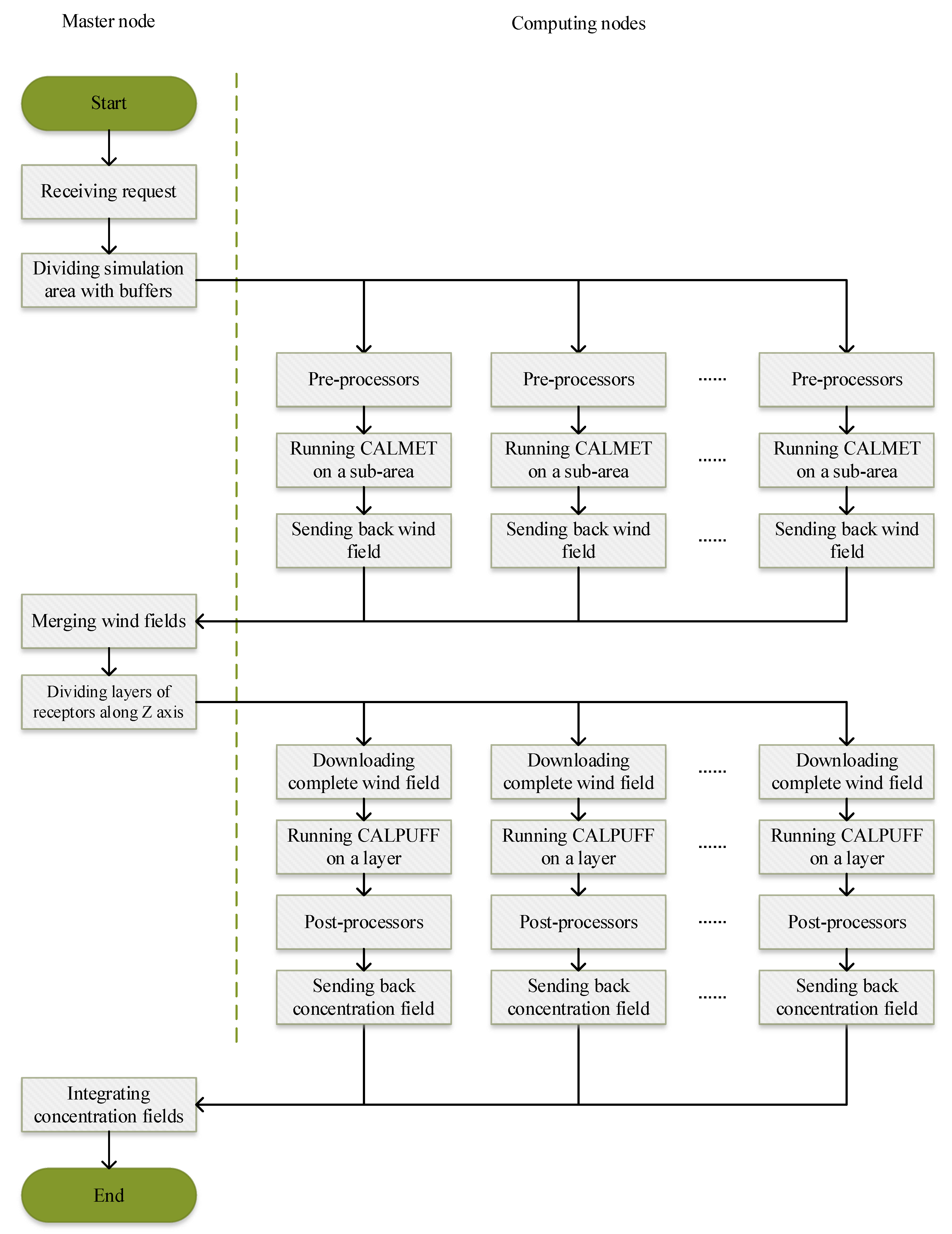
The flow of the parallel algorithm is illustrated in
Figure 5. Assuming that each computing node has obtained the geographic and meteorological data files required by the CALPUFF model in advance, the users of this model only need to specify basic information such as the coordinates of the simulation area and the number of receptors to the master node as a request. The execution of the parallel algorithm is as follows. First, the CALMET module is executed. After receiving the request, the master node calculates the coordinates of each sub-area according to the coordinates of the specified simulation area and the number of divisions. It then sends these coordinates as a message to the public queue of the RabbitMQ exchange, which is monitored by idle computing nodes. When a computing node receives a message from the queue, it executes the computing task according to the sub-area coordinates provided by the message. When a computing task is completed, the computing node sends the URL (uniform resource locator) of the resulting file to the master node through a specific reply queue, and the master node can download the result file through the received URL. After the master node downloads all the sub-area wind fields, it merges these files to obtain the complete wind field file. The CALPUFF module has the same execution process as the CALMET module, except that the message sent by the master node needs to include the URL of the complete wind field file and the computing node needs to download the file through the URL before executing the calculation task.
2.4. Experiment Settings
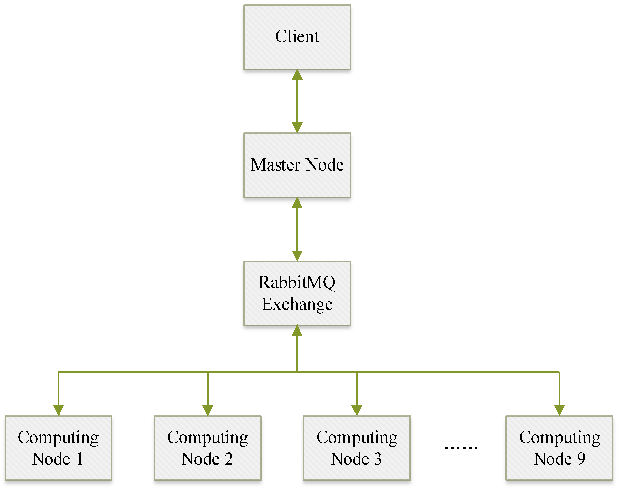
Gas fields are areas with a high risk of toxic gas leakage, and a number of serious accidents have occurred in the past few years. Thus, we used an emergent leakage of natural gas in a high-sulfur gas field in northeastern Sichuan as the simulated experiment, and chose methane as the simulated pollutant. The simulation region is located at Gaoqiao Town (31.36° N, 108.18° E), Kaizhou District, Chongqing, and has an area of 50 km × 50 km with a grid spacing of 1 km. The total simulation time is 2 h, and the time steps of the wind field and the concentration field are both 1 min. The simulation region is divided into 3 × 3 = 9 parts for the CALMET module. Meanwhile, nine layers of receptors are set for the CALPUFF module. The computing cluster used in this paper consists of one master node and nine computing nodes. All the nodes are from the Alibaba Cloud Platform, and each is equipped with an AMD processor (2.55 GHz, 2 virtual CPUs), 4 GB memory, and a 40 GB hard disk. These nodes are connected by a network with a bandwidth of 50 Mbps. The message queue software RabbitMQ is used as the communication middleware. The system architecture is illustrated in
Figure 6.
3. Results
As mentioned in Kleeman 2013, the consistency between the simulation results of the parallel program and the serial program should be verified. Furthermore, it is proposed in Sanjuan 2014 that the solution of the sub-areas must be different from that of the entire area, as the equations in a sub-area cannot take terrain parameters in other parts into account, while the error can be controlled within a certain range via overlapping (buffers). In this article, there is an error in the wind field output by CALMET module as a result of this effect which affects the simulation results. Therefore, we compare the computation time and error corresponding to the buffer sizes.
The computation times of the serial and parallel programs are shown in
Table 2.
In particular, the speedup (the ratio of the time of serial algorithm to the time of parallel algorithm) in Equation (1) and efficiency (the ratio of the speedup to the number of computing nodes) in Equation (2) are exploited to evaluate the effect of acceleration.
In the above equations
is the number of processing units or computing nodes,
is the speedup,
is the efficiency, and
is the computation time. As the speedup increases with the number of computing nodes, it does not fully reflect the performance of the acceleration. The efficiency is an important indicator that reflects whether the speedup increases as expected when the number of computing nodes increases. These data are shown in
Table 3.
We use RMSE (Root Mean Square Error) in Equation (3) and area error in Equation (4) to evaluate the error in the dispersion resulting from the error in the wind field [
11].
In the equations above,
is the RMSE,
is the area error,
is the number of receptors,
is the deviation of the concentration value at the i-th receptor,
is the dispersion range of serial program, and
is the dispersion range of the parallel program. RMSE reflects the numerical error between the simulation result of the serial program and the parallel ones. The accuracy of the extent of dispersion is important in the emergency field as well. We set the output of the CALPUFF to the maximum of one minute average concentrations (for each receptor, we calculate the average concentration once a minute over two hours and record the maximum of the 120 average concentrations), and we define the set of receptors with a concentration greater than zero in the result file as the dispersion range. The data are shown in
Table 4.
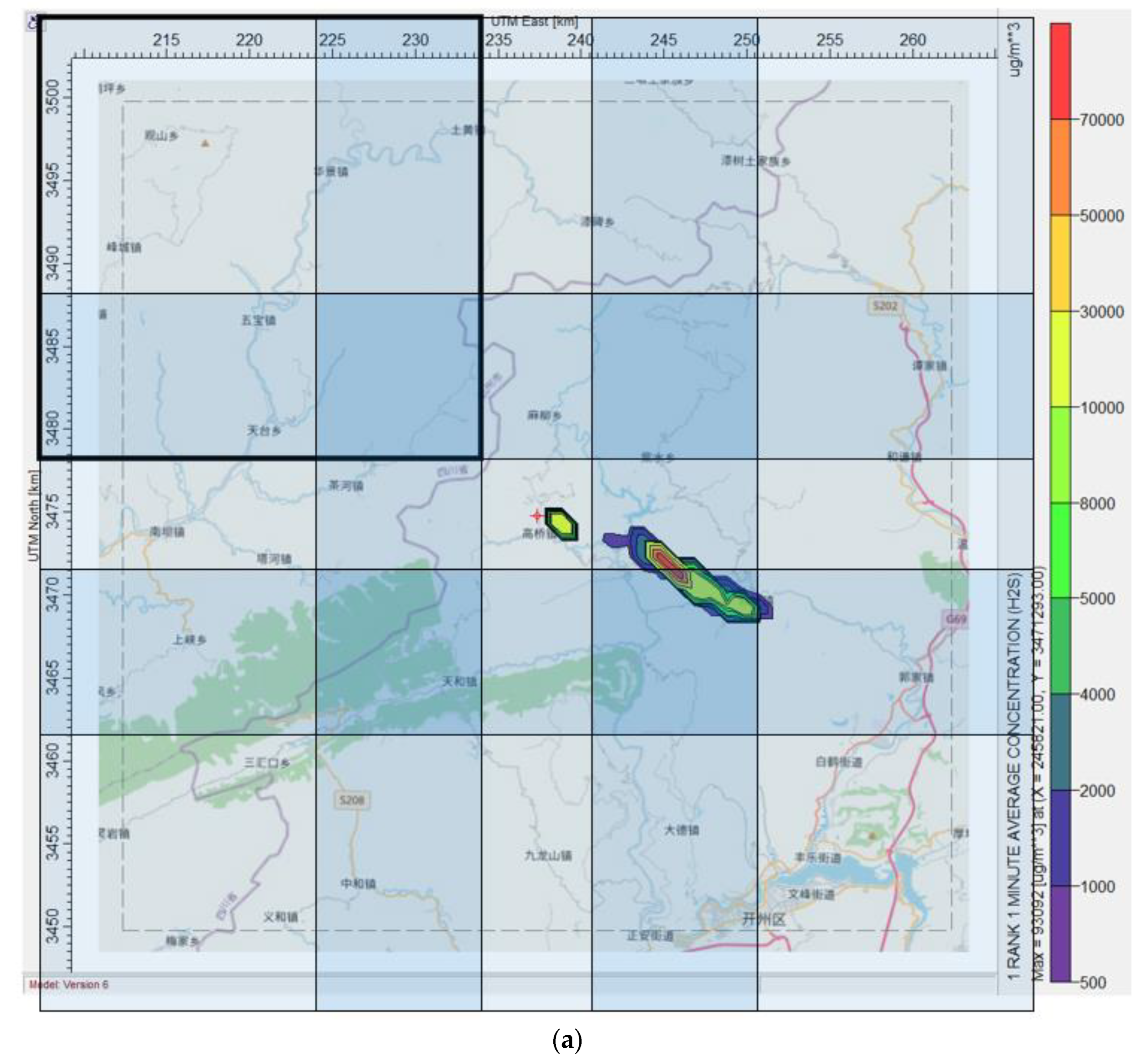
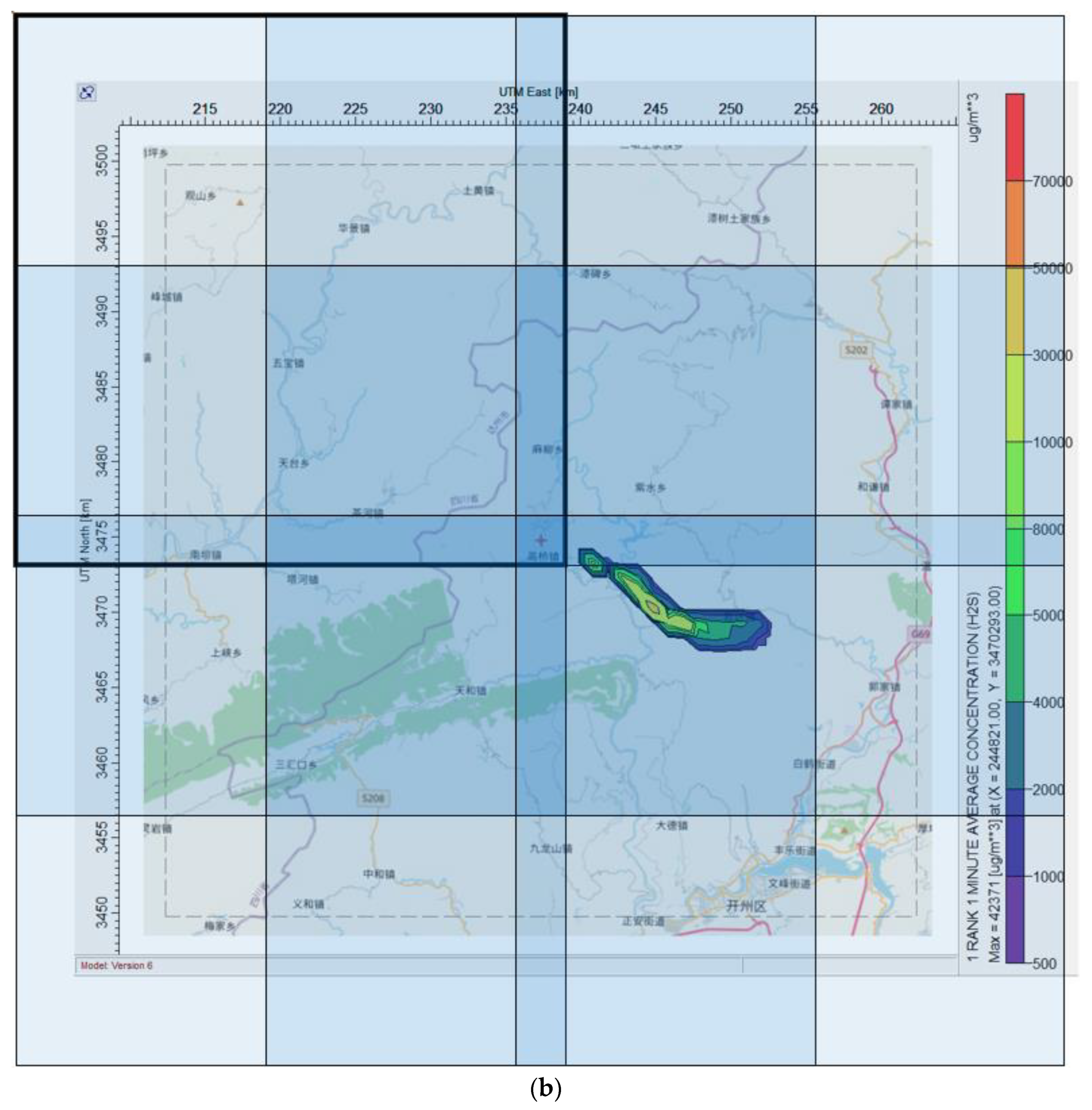
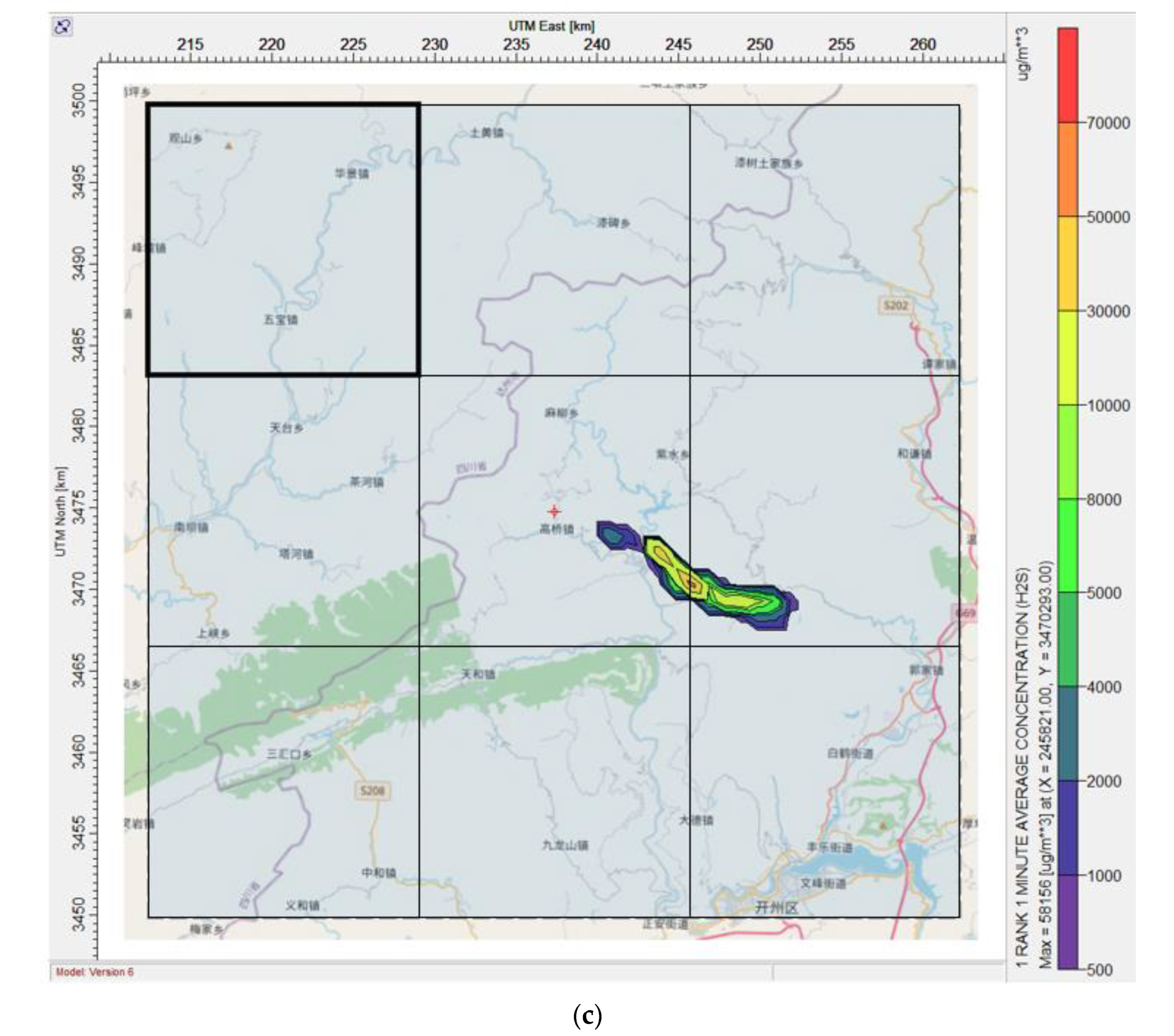
When it is necessary that the area error be less than 1, the methods with a buffer size of 10 and 20 are acceptable. We apply CALPUFF View software to visualize the simulation results of the two and the serial program, as illustrated in
Figure 7.
It can be seen that the values of RMSE and area error are relatively small for the parallel method with buffer size of 20, while the similarity of the dispersion figure of this method to that of the serial program is relatively high. However, from the perspective of computation time, the CALMET module of this method takes 13.20 s, which is greater than 10.74 s with the serial program. This violates the essence of acceleration. Therefore, the method with a buffer size of 10 is most suitable for the simulation case in this article. Its speedup is 6.83, and its efficiency is 75.89%.
4. Discussion and Conclusions
In this paper, a parallel computing algorithm for the emergency-oriented atmospheric dispersion model CALPUFF is designed and evaluated on a cloud platform. The experimental results show that the algorithm is simpler and more efficient than methods using parallel computing interfaces (e.g., MPI, CUDA). Meanwhile, it achieves good acceleration performance in the emergency response case. On a cluster composed of nine computing nodes, the speedup is 6.83 and the efficiency is 75.89%. For an emergency response case with 22,500 computing grid cells and 120 time steps, the computation time on a single computer is about 158.01 s, while the computation time on the cluster is about 23.13 s. Assuming that the emergency response system updates the real-time meteorological data every minute (the same as the time step in the case), the algorithm can ensure that the simulation results are obtained within this minute, which meets the basic needs of emergency response. Such an algorithm is critical to extending the atmospheric dispersion model to the emergency field.
For a model that depends on parameters for the entire simulation area, the computation speed and accuracy are restricted by each other, and a balance between them needs to be found. The method with buffer size of 10 is the most suitable for the simulation case in this article. The speed is too low when the buffer size is greater than 10, and the accuracy is too low when the buffer size is less than 10. When applying the method to real cases, the buffer size should be adjusted according to the actual requirements of speed and accuracy. When an emergency occurs, the parallel program can provide a rough estimate for making responses as soon as possible, then the original program with relative low speed can be implemented to support further decisions.
Note that because the calculation of CALMET in methods with a large buffer is slower than that in the serial program, not parallelizing the CALMET module is an optional method when very high accuracy is required or the computation time of CALMET is not unacceptably long. However, the applicability of this method needs to be further explored, as the conclusions are likely to be different depending on the precise problem being solved (e.g., simulation cases in which the computation time of CALMET is considerably long).
Author Contributions
Conceptualization, M.L. and H.L.; Data curation, D.Y. and M.L.; Formal analysis, D.Y.; Funding acquisition, M.L.; Investigation, D.Y.; Methodology, D.Y.; Project administration, M.L.; Resources, M.L. and H.L.; Software, D.Y. and H.L.; Supervision, M.L.; Validation, D.Y.; Visualization, D.Y.; Writing—original draft, D.Y.; Writing—review and editing, M.L. and H.L. All authors have read and agreed to the published version of the manuscript.
Funding
This work was financially supported by the National Key Research and Development Program of China (Grant Number 2016YFC0803108).
Institutional Review Board Statement
Not applicable.
Informed Consent Statement
Not applicable.
Data Availability Statement
Not applicable.
Acknowledgments
The authors appreciate the help of Rongqian Zhang with visualization.
Conflicts of Interest
The authors declare no conflict of interest.
References
- Kleeman, M.J.; Rasmussen, D.J. Parallel Acceleration of CALPUFF (Version 5.8-Level 070623) Using MPICH-2 Final Report. Available online: https://www.djrasmussen.co/assets/parallel_CALPUFF_FINALreport_CARB.pdf (accessed on 23 March 2020).
- Pinheiro, A.; Desterro, F.; Santos, M.C.; Pereira, C.M.N.A.; Schirru, R. GPU-based implementation of a diagnostic wind field model used in real-time prediction of atmospheric dispersion of radionuclides. Prog. Nucl. Energy 2017, 100, 146–163. [Google Scholar] [CrossRef]
- Cremades, P.G.; Puliafito, E.S.; Fernandez, R.P. GPU Acceleration of CALPUFF. Mecánica Comput. 2010, 29, 7043–7051. [Google Scholar]
- Yao, L.; Wang, Y. Research on Parallel Computing of Air Pollution Dispersion Model Based on MPI. Comput. Eng. 2005, 22, 64–67. [Google Scholar]
- Hu, Y.; Lin, H.; Xu, B.; Zhu, J.; Hu, M. A study on PC cluster based parallel computation of Gauss plume model for multi-point sources. Chin. High Technol. Lett. 2010, 4, 436–440. [Google Scholar]
- Yau, K.H.; Thé, J. A distributed computing solution for CALPUFF. WIT Trans. Ecol. Environ. 2007, 101, 129–134. [Google Scholar]
- Li, M.; Yang, D.; He, W. Comparison and Perspectives on Theories and Simulation Results of Gas Dispersion Models AERMOD and CALPUFF. Geomat. Inf. Sci. Wuhan Univ. 2020, 45, 1245–1254. [Google Scholar]
- Leelőssy, Á.; Molnár, F., Jr.; Izsák, F.; Havasi, Á.; Lagzi, I.; Mészáros, R. Dispersion modeling of air pollutants in the atmosphere: A review. Cent. Eur. J. Geosci. 2014, 6, 257–278. [Google Scholar] [CrossRef]
- Scire, J.S.; Strimaitis, D.G.; Yamartino, R.J. A User’s Guide for the CALPUFF Dispersion Model. Available online: http://www.src.com/calpuff/download/CALPUFF_UsersGuide.pdf (accessed on 28 April 2021).
- Sanjuan, G.; Brun, C.; Margalef, T.; Cortés, A. Determining map partitioning to accelerate wind field calculation. In Proceedings of the 2014 International Conference on High Performance Computing & Simulation (HPCS), Bologna, Italy, 21–25 July 2014; pp. 96–103. [Google Scholar]
- Sanjuan, G.; Brun, C.; Margalef, T.; Cortés, A. Determining map partitioning to minimize wind field uncertainty in forest fire propagation prediction. J. Comput. Sci. 2016, 14, 28–37. [Google Scholar] [CrossRef]
| Publisher’s Note: MDPI stays neutral with regard to jurisdictional claims in published maps and institutional affiliations. |
© 2022 by the authors. Licensee MDPI, Basel, Switzerland. This article is an open access article distributed under the terms and conditions of the Creative Commons Attribution (CC BY) license (https://creativecommons.org/licenses/by/4.0/).


