Article

Effects of Sea-Surface Temperature, Cloud Vertical Structure and Wind Speed on Temperature Change between Hiatus and Post-Hiatus Periods in Tropical Western Pacific

Graduate Institute of Communication Engineering, National Taiwan University, Taipei 10617, Taiwan
*
Author to whom correspondence should be addressed.
These authors contributed equally to this work.
Atmosphere 2022, 13(12), 2130; https://doi.org/10.3390/atmos13122130
Submission received: 28 November 2022 / Revised: 7 December 2022 / Accepted: 15 December 2022 / Published: 19 December 2022
(This article belongs to the Section Biosphere/Hydrosphere/Land–Atmosphere Interactions)

Abstract

:
A region in the tropical western Pacific is selected to study the notable change in temperature between the recent warming hiatus period and the post-hiatus period. In total, three probable factors, namely sea-surface temperature (SST), cloud vertical structure (CVS) and wind speed, which may account for the temperature change are found to exhibit noticeable differences between these two periods. A one-dimensional atmospheric radiative transfer model, incorporating convective adjustment and energy exchange with the ocean, is developed to simulate the diurnal pattern of temperature profile under the influence of the three probable factors in the two concerned periods. Virtual profiles of sea-surface temperature, cloud vertical structure and wind speed in both periods are developed from data available in the literature. Diurnal patterns of temperatures near the air–sea interface are computed with the proposed model over a sufficient number of days. The simulated temperatures under different combinations of factors, in either the hiatus or post-hiatus period, are statistically analyzed to gain insights about the separate and combined effects of these three factors on causing climate change.

1. Introduction

Global warming and climate change have attracted broad attention from the general public and the scientific community, for their potential impact on human societies and ecological environments. The Intergovernmental Panel on Climate Change (IPCC) delineates global warming as an increase in global mean surface temperature (GMST) from the pre-industrial level [1]. It was reported that more than half of the GMST increase between 1950–2010 could be attributed to human activities [2].
The long-term trend of GMST since the last century indicates that the warming rate is not constant. Periods of remarkable warming rate were interspersed with periods of slow warming rate, and the underlying mechanism is not well understood. The periods of slow warming rate are usually referred to as global warming hiatus or hiatus. Several climate phenomena across different spatial and temporal scales maybe interrelated, including El Ni n ˜ o-southern oscillation (ENSO), Pacific decadal oscillation (PDO), interdecadal Pacific oscillation (IPO), and so on. However, none of these phenomena alone can account for the whole trend [3,4].
A recent warming hiatus period was reported to last from 1998 to 2013 [3] and we are now in a post-hiatus period since the end of the recent hiatus. Some research works suspected this hiatus was mistakenly labeled due to artifacts in the temperature record [5]. Other studies revealed notable changes in sea-surface temperature (SST), wind condition, and other climate variables [6]. In spite of the disagreement, investigations on the energy budget of Earth-atmosphere climate system at the top-of-atmosphere (TOA) showed a net energy gain during this hiatus period, and the excess energy that did not contribute to the increase in SST might have been absorbed by the ocean [7].
Clouds play an important atmospheric role given that they cover around 70.8% of the global sky [8]. Clouds can cool the atmosphere by partially reflecting solar irradiance back out to space [9]. Clouds can also warm the atmosphere via the greenhouse effect by absorbing more longwave radiation from below and emitting less at the top [9]. The effects of clouds on the climate system depends on the cloud type, properties, location, and occurrence rate [8].
In terms of layer number in a cloud system, the most common single-layer cloud covered about 41% of the global sky, two-layer clouds were observed about 21.8%, followed by three-layer clouds at 6.3% and four-layer clouds at 1.7% [10]. In some tropical regions, multilayer clouds can occur above 35% [10]. The high occurrence rate of multilayer clouds may affect regional climate, such as the temperature profile in the tropical troposphere [11].
Clouds present a major source of uncertainty in climate modeling, and thus a better understanding of the interaction between clouds and other environmental factors will help increase the credibility of climate modeling. To the best of our knowledge, although studies focusing on the cloud effect in hiatus are relatively rare, there have been numerous inspirational studies conducted that address the variation of cloud properties under warmer global conditions.
Many recent studies explored the variation of clouds under climate change, including the distribution of cloud cover and occurrence rate, either globally or regionally. Increased global mean cloud cover was found between 2003–2012 [12]. A study on cloud cover of specific types revealed that low-lying clouds decreased under global warming [13]. Cloud cover was found to generally increase over land and decrease over seas [12]. A study on tropical land-based regions suggested a reduction in the number of clouds [14]. Another study conducted around the Arctic sea concerning future sea ice loss in a warmer world suggested an increase in cloud cover during non-summer seasons [15]. Different warming patterns lead to various changes in regional cloud cover [16], and these changes may amplify global warming [17].
Under a warmer climate, the cloud vertical structure (CVS) was found shifted upwards [18], high clouds were also shifted upwards [19], and tropical high clouds were time-shifted towards noon [20].
Many climate models have been developed to address different problems of varying complexity. Nowadays, numerical climate models based on physics are indispensable for studying various climate change scenarios such as global warming. The one-dimensional radiative–convective model (1D-RCM) is a numerical model that has been widely used to study climate-related problems, owing to its simplicity and efficacy in studying the first-order reaction of the climate system [21,22,23,24,25]. In 1D-RCM, the atmosphere is approximated as parallel planar layers from the top of atmosphere (TOA) to the bottom of air, and the vertical temperature profile is determined by radiative transfer and heat convection.
Regarding temperature profiles in the ocean region, the effects of sea-surface temperature (SST) and wind have received more attention than those of clouds, with the clouds being characterized by cloud cover instead of cloud vertical structure. The variation in cloud vertical structure (CVS) was rarely addressed in previous studies on warming hiatus. Hence, we are motivated to study the variation in CVS in the tropical western Pacific (TWP) region before and after the end of the recent hiatus. This work presents the effects of CVS variation on the temperature profile in the TWP region for the first time, and compares these effects with those from the variations in SST and wind. To achieve this, a rigorous physical model based on a line-by-line 1D-RCM is developed to simulate the diurnal variation of temperature profiles under the combined effects of varying CVS, SST, and wind systematically. The variations of these three factors are derived from long-term data before and after the end of the recent hiatus. A shortage of diurnal measurement data is avoided, and data bias due to extreme or unexpected weather conditions is also mitigated. The simulation results are statistically analyzed to gain additional understanding and insights on the individual and composite effects of these three factors.
More specifically, a semi-analytic approach, incorporating key physical mechanisms, is proposed and applied on the tropical western Pacific region where the weather pattern is more regular. The profiles of air composition, moisture, and clouds are simulated based on their long-term statistical features. Hence, the diurnal variation of temperature profile can be simulated in a more controllable manner, conducive to better observing the impacts of three probable factors, sea-surface temperature, wind and cloud vertical structure. The simulated diurnal variation of near-surface temperature can help recreate the global warming effect, and the subsequent statistical analysis provides a creditable evaluation on the underlying physical mechanisms.
Real air–sea interactions are more complicated than those modeled and simulated in this work. However, the results in this work well-manifest the underlying physical mechanisms and may inspire some insights for further studies on climate problems involving air–sea interactions. Variations in sea-surface temperature are known to modulate the marine atmospheric boundary layer (MABL) and affect the wind field, which was explored over the Southern Ocean [26], the California current system [27] and the midlatitude regions [28]. Diurnal variations in sea-surface temperature are known to affect the formation of clouds [29], which can be better understood if the complicated air–sea interactions are taken into account [29,30].
The rest of this paper is organized as follows. In Section 2, the hiatus and post-hiatus periods as well as the region of interest (ROI) are delineated. In Section 3, the variation in cloud vertical structure between hiatus and post-hiatus periods in the tropical western Pacific is analyzed. In Section 4, the simulation scenario, relevant parameters, and the three probable factors are orchestrated and justified. The simulations results are discussed in Section 5, and some conclusions are drawn in Section 6.

2. End of Recent Hiatus and Region of Interest

In this Section, we will first discuss how to determine the end of recent hiatus period, which is also the beginning of the post-hiatus period. Then, we will discuss how to choose the region of interest and the motivation behind this study. A table listing the region of interest in this study will be given at the end of this Section.

2.1. Determining the End of Recent Hiatus

The Intergovernmental Panel on Climate Change (IPCC) used the global mean surface temperature (GMST) over lands and oceans as a metric to estimate the trend of global warming [1]. Figure 1 shows the anomaly of GMST between 1920–2020, with respect to the average value between 1951–1980, provided by the Goddard Institute for Space Studies Surface Temperature product version 4 (GISTEMPv4) [31,32], which includes the land measurement data in the Global Historical Climatology Network (GHCN) version 3 and version 4 [5,32], and the sea measurement from the Extended Reconstructed SST version 5 (ERSSTv5) product [32], providing monthly SST anomaly [33].
As shown in Figure 1, the GMST does not increase at a constant rate. The shaded areas mark the hiatus periods with relatively lower rate of temperature increase. A recent hiatus ended near 2014.
Figure 2 shows the Pacific decadal oscillation (PDO) index and the Tripole index (TPI), respectively, between 1920–2020. The PDO index is derived from the SST anomaly in the northern Pacific [34], which is the leading principal component (PC) or empirical orthogonal function (EOF) of the mean SST anomalies, from November to March, in the Pacific Ocean to the north of 20 ° N latitude [35].
The TPI index is derived from the SST anomalies over the tripole of central equatorial Pacific, northwest Pacific and southwest Pacific regions, which are the centers of SST anomalies in decadal time scale, known as the interdecadal Pacific oscillation (IPO) [36]. Figure 1 and Figure 2 show the correlation between the PDO index, the TPI index, and the GMST in manifesting the recent hiatus period. The PDO and TPI indices recorded in the hiatus periods between 1943–1976 and 1998–2014 were mostly negative, while those recorded in the warming speed-up periods between 1976–1998 and after 2014 were mainly positive.
Figure 3 shows the PDO index [34] and the TPI index [36] between 2006–2018, where a phase transition from negative to positive appeared in the spring of 2014. Hence, we set February 2014 as the end of recent hiatus and March 2014 as the beginning of current post-hiatus period. In the simulations of this work, parameters featuring the hiatus period from March 2006 to February 2014 are labeled with h, and those in the post-hiatus period from March 2014 to February 2019 are labeled with p.

2.2. Region of Interest in This Study

Figure 4a shows the mean sea-surface temperature anomalies, Δ SST d = Δ SST p Δ SST h (K), which are derived by taking the average of the ERSSTv5 monthly data in 2 ° × 2 ° gridboxes, over the period from 1971–2000 [33]. A net increment in SST in the region of interest is observed after the hiatus period.
Figure 4b shows the difference in cloud radiative effect, Δ CRE net (W/m 2 ), at TOA between the hiatus period and the post-hiatus period [37], where Δ CRE net = Δ CRE SW + Δ CRE LW , Δ CRE α = CRE α , p CRE α , h with α = SW, LW, CRE α , p and CRE α , h are the CRE averaged over the post-hiatus and hiatus periods, respectively. Figure 4c,d show Δ CRE SW (W/m 2 ) and Δ CRE LW (W/m 2 ), respectively, at TOA.
In this work, a region of interest (ROI) in the tropical western Pacific is enclosed with a rectangle, with the corner coordinates ( ϕ lat , ϕ lon ) = ( 2 . 50 ° N, 165 ° E), ( 2 . 50 ° N, 170 ° W), ( 7 . 50 ° S, 170 ° W) and ( 7 . 50 ° S, 165 ° E), respectively.
The region of interest is chosen since it bears negative Δ CRE SW (cooling by SW) and positive Δ CRE LW (warming by LW) after the hiatus period, which may be related to the change in cloud vertical structure in this region. The net effect is negative Δ CRE net , which implies cooling at TOA. Compared to Δ CRE SW and Δ CRE LW , the magnitude of Δ CRE net is relatively small. Hence, we will explore a possible connection between the variation in cloud vertical structure in this region to the variation in these Δ CREs.
Table 1 lists the region of interest and time windows in this study.

3. Variation of Cloud Vertical Structure in ROI

3.1. CVS Observed by CloudSat and CALIPSO

A CloudSat was jointly launched with a cloud-aerosol lidar and infrared pathfinder satellite observations (CALIPSO) in 2006 and joined the Afternoon Constellation [38]. A W-band (94 GHz) cloud-profiling radar (CPR) on CloudSat and a cloud-aerosol lidar with orthogonal polarization (CALIOP) at 530 nm a nd 1060 nm (on board CALIPSO) jointly collected data on cloud vertical profile [38]. The lower sensitivity of the CPR on small particles can be complemented by the CALIOP to acquire low-layer water cloud and subvisual cirrus at finer resolution [39].
This joint radar-lidar system is capable of classifying clouds, in terms of their height and optical properties, into 9 types [38]. The resolved cloud types from the observed profiles over the satellite flypass swath are stored in the CloudSat 2B-CLDCLASS-lidar data product [40], which facilitate studies on the global distribution of different types of clouds [10].
Figure 5 shows the cloud types in the CloudSat 2B-CLDCLASS-lidar product [40]. The nine cloud types are cirrus (Ci), altostratus (As), altocumulus (Ac), stratus (St), stratocumulus (Sc), cumulus (Cu), nimbostratus (Ns), deep convection (DC) and multi-layered cloud (ML). The satellites flew by the equator twice per day, once during the daytime and once at night-time. However, after a battery malfunction in 2011, the onboard instruments for observing the cloud vertical structure could operate only during the daytime flypass [38]. Hence, we use only the daytime data for the comparison between hiatus and post-hiatus periods.
The occurrence rate of a given cloud type c in this study is defined as the ratio between the number of matched samples, S c , and the total number of samples observed in the ROI from the CloudSat 2B-CLDCLASS-lidar product. Explicitly, for cloud type c,
F h c = hiatus ROI S c hiatus ROI c S c . F p c = post hiatus ROI S c post hiatus ROI c S c .
where F h c and F p c are the occurrence rates in hiatus and post-hiatus periods, respectively, and Δ F c = F p c F h c denotes the difference of occurrence rates between these two periods.

3.2. Occurrence Rate of CVS in ROI

Table 2a–d list the occurrence rate of CVS features by observations. Table 2a lists the occurrence rate of cloud layer number in the hiatus period ( F h ) and the difference Δ F = F p F h with that in the post-hiatus period ( F p ), where 0 represents a clear sky. Single-layer clouds were observed most frequently (41.91%), followed by double-layer clouds (24.03%), clear sky (23.38%), and clouds with three or more layers (10.68%).
Compared with the hiatus period, the occurrence rate of clear sky in the post-hiatus period decreases by 4.09%, two-layer cloud increases by 2.58%, more-than-two-layer cloud increases by 3.18%, and single-layer cloud drops by 1.68%.
Table 2b lists the occurrence rate F h and Δ F of single-layer cloud. In the hiatus period, among the 41.91% of single-layer cloud, Ci takes 20.98%, Cu takes 14.30%, and all the other types take 6.63%. The decrease of single-layer cloud ( 1.68 %) in the post-hiatus period is resulted from the decrease of low clouds, including Sc ( 0.62 %) and Cu ( 4.00 %), and the increase of other cloud types with higher cloud tops, including Ci (0.59%), As (0.92%), Ac (0.25%), Ns (0.38%) and DC (0.81%).
Table 2c lists the occurrence rate F h of double-layer cloud, where each row refers to a bottom cloud type and each column refers to a top cloud type. Among the 24.03% of double-layer cloud, 22.14% come from the first column, with Ci as the top layer.
Table 2d lists the occurrence rate F h and Δ F of bottom cloud type in double-layer clouds, with Ci as top cloud. In the hiatus period, the dominant types of bottom cloud are Ci (5.80%), Cu (10.05%), Ac (2.57%) and As (1.52%), respectively. The occurrence rates of low cloud types as the bottom layer generally decrease, including St ( 0.01 %), Sc ( 0.17 %) and Cu ( 0.72 %); while those of cloud types with higher cloud top as the bottom clouds generally increases, including Ci (0.90%), As (0.68%), Ac (1.03%), Ns (0.24%) and DC (0.29%).
From the observation on the single-layer clouds in Table 2b and the double-layer clouds in Table 2d, similar distinction of Δ F by the cloud types was observed. Negative trends are related to those clouds with lower cloud tops, including St, Sc and Cu; while other clouds with higher cloud tops show positive trends. Hence, we will regroup the occurrence rates in labels of low, middle and high cloud types to simplify the simulation design and comparison between hiatus and post-hiatus periods.

3.3. Occurrence Rate of Regrouped CVS in ROI

Table 3 lists the regroup of cloud types used in the simulations. Based on the number of layers, clouds are regrouped into three sky conditions, namely clear sky (CL), single-layer cloud (SL), and multi-layer cloud (ML). Among the ML cloud types, double-layer cloud has relatively high occurrence rate, as shown in Table 2a. Hence, double-layer cloud type is used to represent ML in the simulations. Based on the altitude of cloud tops, the cloud types in Figure 5 are regrouped into high cloud (HC), middle cloud (MC) and low cloud (LC).
Table 4a–c lists the F h and Δ F after regrouping the data in Table 2a,b,d, respectively. Table 4a lists the occurrence rate F h and Δ F of sky condition after regroup. SL is the most popular sky condition in the hiatus period (41.91%), followed by ML (34.71%). In the post-hiatus period, ML becomes the most popular one (40.48%), followed by SL (40.23%). CL is the least popular sky condition, 23.38% in the hiatus period and 19.29% in the post-hiatus period, which implies an increase of cloudiness by 4.09% after entering the post-hiatus period.
Table 4b lists the occurrence rate F h and Δ F of regrouped single-layer clouds. It is observed that LC decreases by 4.63%, MC increases by 1.55% and HC increases by 1.40%, resulting in a decrease in SL of 1.68%.
Table 4c lists the occurrence rate F h and Δ F of regrouped bottom-cloud type in double-layer clouds, with Ci as the top cloud. Similar to the data listed in Table 4b, the occurrence rate of regrouped types of bottom clouds in double-layer cloud shows a decrease in LC ( 0.90 %) and increases in MC (1.95%) and HC (1.19%), resulting in a net increase of ML (double-layer clouds with Ci as the top cloud) by 2.24% as listed in Table 2d. In the post-hiatus period, the occurrence rate of bottom cloud being MC or HC is 14.05%, surpassing that of bottom cloud being LC (10.33%).

3.4. Summary of Observation Data in ROI

By inspecting the observation data in the ROI, we obtain three key points on CVS after the end of recent hiatus. The first point is the increase in cloudiness, manifested by the decrease in CL in Table 4a. The second point is the increase in average number of cloud layers. The increased cloudiness is not attributed to the increase in single-layer clouds but rather the increase in clouds with two or more layers, as shown in Table 2a and Table 4a. The third point is the upward shift of clouds, manifested by the decrease in LC and the increase of MC and HC, in both single-layer and double-layer clouds shown in Table 4b,c.
The variation in CVS in the ROI may be correlated with the increase in sea-surface temperature (SST) shown in Figure 4a. Note that the cloudiness was reported to be negatively correlated with SST in [41]. The negative correlation between SST and LC reported in [42] is consistent with our finding that the increase in SST, as shown in Figure 4a, is correlated with the decrease in LC. The correlation between SST and the occurrence rate of ML clouds is seldom discussed in the literature.
The variation in CVS in the ROI is consistent with the cloud radiative effect at TOA shown in Figure 4c,d. The cooling effect in SW at TOA, as indicated by negative Δ CRE SW in Figure 4c, may be due to the increase in cloudiness, which reflects more sunlight back out to space. The warming effect in LW at TOA, as indicated by positive Δ CRE LW in Figure 4d, maybe caused by the upward shift of the CVS. Higher clouds tend to trap more LW than lower clouds, hence an upward shift in CVS can trap more LW and induce a warming effect.

4. Design of Simulation Scenarios

In this section, we will simulate the effects of cloud vertical structure (CVS) on the sea-surface temperature and the air temperature above it, which are the most important environmental parameters directly affecting our lives and activities. The effects of CVS difference between the hiatus and post-hiatus periods on the near-surface temperatures will be compared with those from other two factors, sea-surface temperature and wind speed. All these three factors are related to energy exchange. The CVS affects energy exchange in a regional atmospheric column, the wind speed affects the transport of energy between neighboring columns, and the sea-surface temperature is a metric of energy reservoir over a large area. Next, we will prepare the simulation model of the three probable factors and the other input parameters required for the simulations.

4.1. Simulation Model of Probable Factors

The three probable factors, the foundation sea-surface temperature (SST fdn ), cloud vertical structure (in terms of occurrence rate F c ) and wind speed ( v a 10 ), that may differentiate the sea-surface temperature and nearby air temperature between hiatus and post-hiatus periods are put together for simulations.
Figure 6 shows the average sea-surface temperature at 6 AM local time (LT) in the hiatus and post-hiatus periods, labeled as SST fdn , h and SST fdn , p , respectively. They are derived from the ERA5 dataset [43], under the assumption that the depth profile of ocean temperature at 6 AM LT is laterally homogeneous [44]. It is observed that the temperature during the post-hiatus period is higher than in that of its hiatus period counterpart by 0.5 to 1 K. The temperature difference is slightly larger in the first six months than in the subsequent six months.
Figure 7a shows the average wind speed in the hiatus period, v a 10 , h (m/s), derived from the ERA5 [43]. Figure 7b shows the difference of average wind speed, v a 10 , p v a 10 , h (m/s) [43]. It is observed that v a 10 , p is smaller than v a 10 , h in each month and at all local times.
To make the correlation between temperature difference and the variation in CVS traceable in the simulations while keeping the simulated CVS compatible with the observation data, the CVS is categorized into six prototypes listed in Table 3, including clear sky (CL), three single-layer clouds (LC, MC, HC), and two double-layer clouds (HC + LC, HC + MC). Note that precipitation is not considered in this work.
Figure 8a–c show the prototypical cloud vertical structures of high cloud (HC), middle cloud (MC) and low cloud (LC), respectively, specified in the simulations. Each prototypical CVS is arbitrarily set to last for 2 h, which is the simulation time step. The parameters of these prototypes, including cloud-top altitude and cloud thickness, are derived from the in situ measurements at Nauru ( 0 ° 31 15 . 6 S, 166 ° 54 57 . 6 E) [45,46], which is located near the northwest corner of the tropical western Pacific. Figure 8d,e show the prototypical CVSs of HC + LC and HC + MC, respectively, which are the superposition of those shown in Figure 8a–c.
Table 5 lists the parameters of cloud types HC, MC and LC, respectively, derived from the in situ measurements [45,46] and the Optical Properties of Aerosols and Clouds (OPAC) package [47]. The ice cloud is characterized by generalized effective size of ice crystal, D ge ( μ m), and ice water content, IWC (g/m 3 ). The water cloud is characterized bu droplet effective radius, r eff ( μ m), and liquid water content, LWC (g/m 3 ).
Table 6 lists the occurrence rate of cloud types in the two periods. The post-hiatus period features more cloudiness, more two-layer clouds, more high clouds and fewer low clouds. In each time step of simulations, the cloud type is randomly picked following the occurrence rate.

4.2. Justification of Methodology to Simulate Diurnal Variation

In this work, we propose an innovative approach to acquire long-term statistics on near-sea-surface temperatures by simulating the diurnal patterns of relevant parameters over a sufficiently long period of time. In order to achieve this, we developed a modified 1D radiative-convective model (RCM) to compute the temperature profile that changes continuously with the local time.
The 1D-RCM has the merit of being less sensitive to fluctuations in the input data. A more complex model is prone to triggering chaotic output with slight input data fluctuations. The 1D-RCM was originally used to predict an equilibrium state of the Earth’s atmosphere, providing pilot results to speculate possible relations between the concentration of greenhouse gas and the rise in Earth’s temperature.
The modified 1D-RCM in this work includes the most significant mechanisms that contribute to the temperature variation and is less sensitive to input data fluctuations. It is not intended for weather-type predictions. Instead, it is used to produce a steady-state or climate-like diurnal pattern of temperature based on the diurnally varying environmental parameters. In this context, weather-like diurnal patterns refer to those more susceptible to interruptions from drastic weather events such as a storm or hurricane. On the other hand, climate-like diurnal patterns refer to the long-term steady-state diurnal patterns without the impact of drastic short-term weather events. Our simulation approach has the merits of excluding irrelevant factors from the model and focusing on the effects of the most probable factors.
The long-term statistical data of wind speed and foundation sea-surface temperature in the hiatus and post-hiatus periods are used in the simulations. Prototypical cloud vertical structures are inducted from available measurement data, and their occurrence over various time slots during the day is arranged according to the probability distribution derived from the historical data during these two periods. In this manner, drastic weather events are neglected or smoothed out in the simulations. The long-term impact of these three factors are compared by using the statistical data derived from the simulated diurnal pattern of temperature over a sufficiently long time period.
The resulting diurnal patterns of near-surface temperatures are statistically analyzed to predict the long-term trend, analogous to how a long-period weather record is statistically analyzed to predict the long-term climate trend. In the past and in recent times, records of such fine temporal resolutions were not available. The expedient approach proposed in this work simulates virtual data that inherit the same statistical features as in the available sparse data.

4.3. 1D-RCM and Relevant Parameters

In the modified 1D-RCM proposed in this work, the convection adjustment scheme is modified by incorporating heat flux exchange at the air–sea interface, allowing discontinuity between air and sea-surface temperatures. The implementation of this model, with diurnal variation of relevant parameters, is presented in Appendix A.
In total, three major greenhouse gases are included, namely water vapor, carbon dioxide and ozone. The carbon dioxide concentration and the vertical profiles of water vapor and ozone are derived from the radiative–convective equilibrium model intercomparison project (RCEMIP) [48]. The absorption is composed of line absorption [9,49,50] and continuum absorption [51,52,53]. The scattering is contributed to by the air [54] and cloud layers [55,56,57].
To account for the diurnal variation of solar zenith angle, the time step in our simulations is set to two hours, which represents a trade-off between the desired time resolution and the confidence in sparse data. The cloud vertical structure was measured once daily as discussed in Section 3.1. The weather patterns in the tropical Pacific do not change abruptly with time, hence a time slot of two hours seems reasonable. The cut-off solar zenith angle is set to θ cut = 88 ° when encompassing short-wave radiation at a local time [58]. The air–sea interface is assumed to be a Lambertian surface, featuring albedo of α = 0.06 and emissivity of ϵ = 1 , without loss of generality.

5. Simulation Results and Discussions

In this section, diurnal variation of temperature profile and relevant parameters will be simulated over a sufficient number of days to acquire statistically significant results.
Table 7 summarizes the feature change of three probable factors in the hiatus and post-hiatus periods. The three factors (SST fdn , F c and v a 10 ) compiled in Section 4.1 will be used to simulate two benchmark cases to characterize the hiatus period and the post-hiatus period, respectively. Subsequently, one of the three factors will be swapped between the two benchmark cases to highlight the effects of the swapped factor. Next, two of the three factors will be swapped between the two benchmark cases to highlight the combined effects of the two swapped factors. Finally, we will compare the simulation results among these cases and evaluate the potential of these three factors in altering the regional warming tendency.

5.1. Benchmark Cases of Hiatus and Post-Hiatus Periods

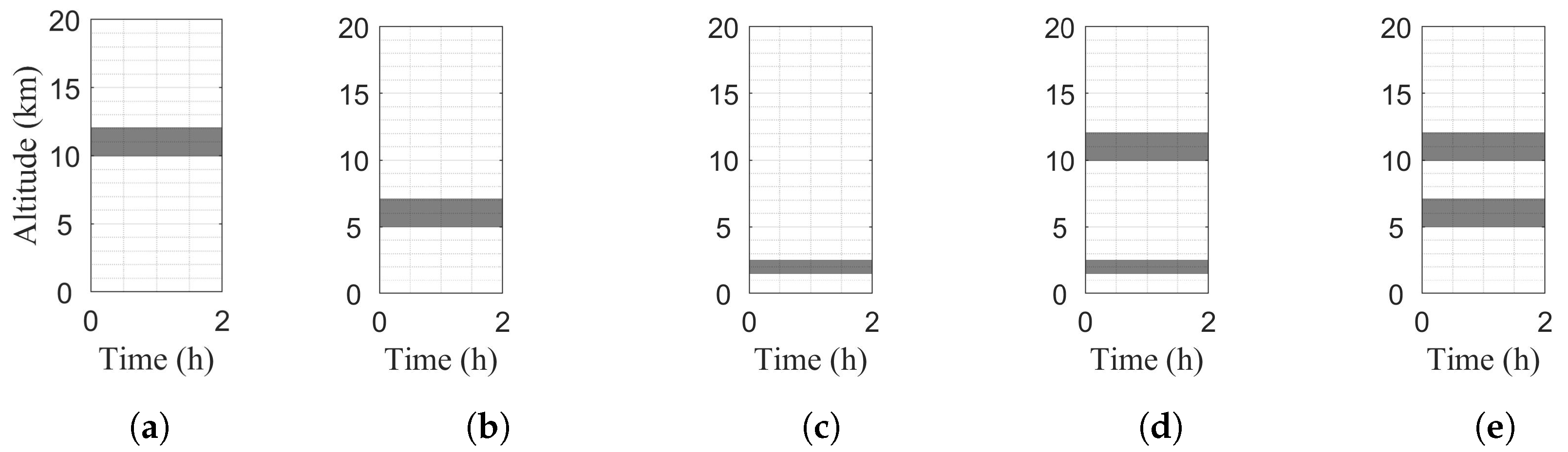
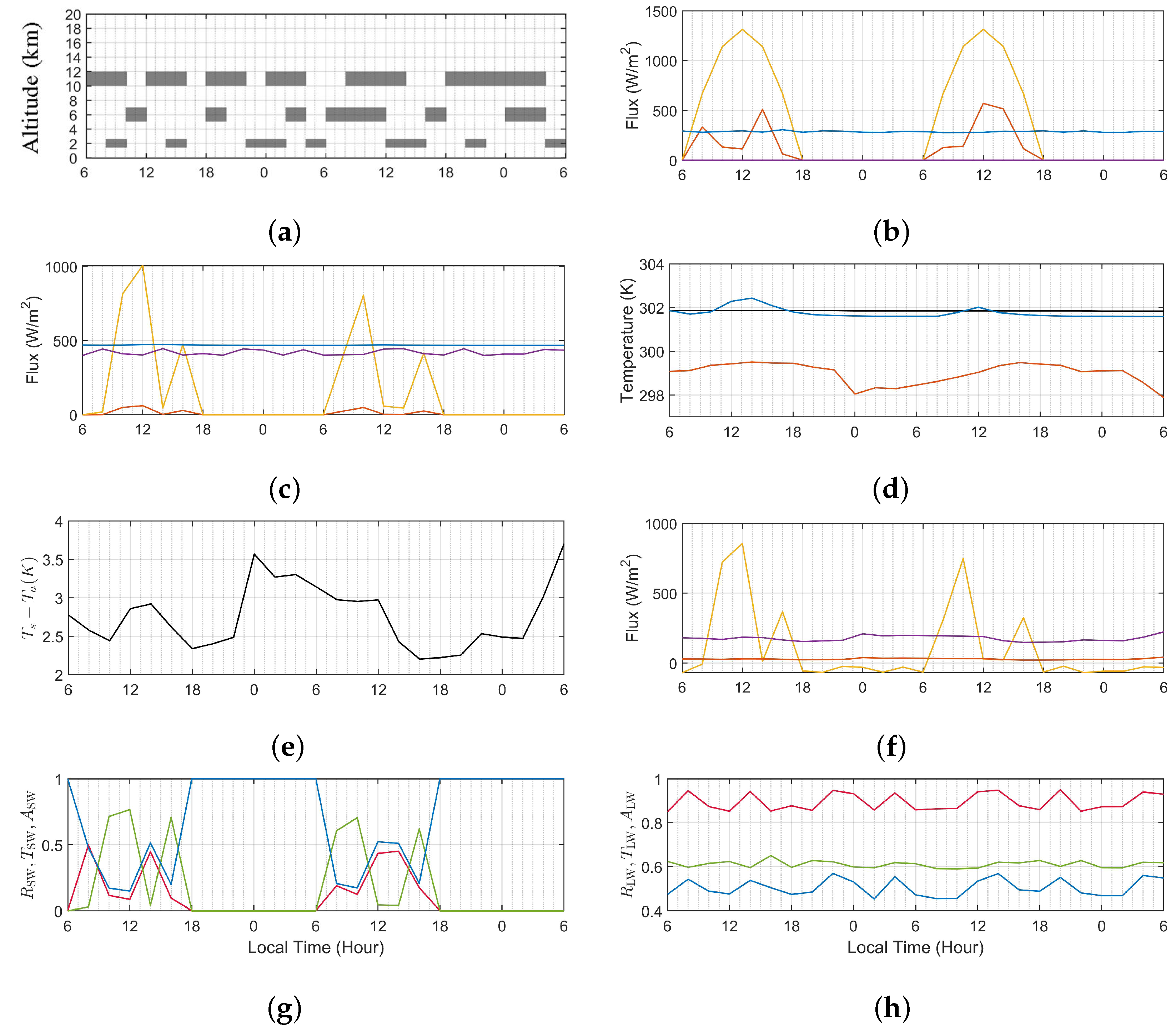
Figure 9 shows the simulation results over 48 h in hiatus period, from day 1, 6 AM LT (d1h6) to day 3, 6 AM LT (d3h6). Figure 9a shows the simulated cloud pattern for these two days. Figure 9b shows the radiative flux densities at TOA, where J SW and J LW are the simulated downward SW and LW fluxes, respectively, and J SW and J LW are the simulated upward SW and LW fluxes, respectively. Figure 9c shows the radiative flux densities at the air–sea interface. Figure 9d shows the temperature near the air–sea interface, where T s is significantly correlated with J SW reaching the surface, as shown in Figure 9c. Figure 9e shows the variation of T s T a is mainly affected by T a , since T a varies over a wider range than T s due to the lower heat capacity of air compared to water.
Figure 9f shows the net downward radiative flux R surf entering the ocean, sensible heat flux H and latent heat flux L e , respectively, at the air–sea interface. Both H and L e are positive when moving upwards. Comparison with the diurnal variation of temperature in Figure 9d suggests that the ocean is heated up by R surf after sunrise, with the daily maximum T s lagged behind the daily maximum R surf . As T s rises, T s T a also increases to pump in more H and L e into the air. As T s begins to drop from its daily maximum, T a keeps rising to reduce T s T a until the net energy absorbed in the atmospheric boundary layer becomes zero, then T a begins to drop. As a result, the daily maximum T a also lags behind the daily maximum T s .
Near sunset, both T s and T a continue to decline. When T s is constrained by SST fdn , T a keeps dropping due to lower heat capacity of air than water, resulting in a second peak of T s T a in one day. Note that either T s or T a displays one daily peak in general, T s T a displays two daily peaks, with the second peak higher than the first one. The first peak is due to the rise of T s , which is small, the second peak is due to the decline of T a , which is relatively large. The second peak of T s T a also leads to the increase of H and L e during the night-time. As shown Figure 9f, H and L e play more important roles to transport energy from ocean to atmosphere during the night-time when the radiative flux is weak.
In order to quantify how the clouds affect shortwave radiation (SW), define three indices as
R SW = J SW , toa / J SW , toa , J SW , toa 0 0 , J SW , toa = 0 T SW = J SW , surf / J SW , toa , J SW , toa 0 0 , J SW , toa = 0 A SW = 1 R SW T SW
where R SW is the ratio of SW flux reflected back to space at TOA, T SW is ratio of SW flux passing from TOA to the air–sea interface, and A SW is the ratio of SW flux absorbed in the atmosphere.
Correlation is observed between the indices ( R SW , T SW , A SW ) shown in Figure 9g and the cloud pattern shown in Figure 9a. For example, A SW R SW > T SW with clouds HC + LC at d1h8, d1h14 and d2h12; T SW > A SW R SW with clouds HC + MC at d2h8 and d2h10, as well as with cloud MC at d1h10 and d2h16.
By scrutinizing more time steps, it is found that the cloud patterns can be sorted into two groups based on their correlation with the indices ( R SW , T SW , A SW ). The first group has the feature of T SW > A SW R SW , with large portion of SW reaching the air–sea interface, for example, CL at d1h16, HC at d1h12, MC at d1h10 and d2h16, and HC + MC at d2h8 and d2h10. The second group has the feature of A SW R SW > T SW , with large portion of SW either absorbed in the atmosphere or reflected back to space, for example, LC at d2h14 and HC + LC at d1h8, d1h14 and d2h12. The LC in the second group, either by itself or as part of HC + LC, appears to play an important role in refraining SW from reaching the air–sea interface.
Note that J SW , surf is the main heating source of T s , and cloud types LC and HC + LC have higher occurrence rate in the hiatus period than in the post-hiatus period, as listed in Table 4d, the SW flux has stronger tendency to raise T s in the post-hiatus period than in the hiatus period.
Similarly, to quantify how the clouds affect longwave radiation (LW), define three indices as
R LW = J LW , surf / J LW , surf T LW = J LW , toa / J LW , surf A LW = R LW + T LW 1
where T LW is ratio of LW flux passing from the air–sea interface to TOA, R LW is the ratio of LW flux reflected back to the air–sea interface, and A LW is the ratio of LW flux contributed by the atmosphere to the air–sea interface. Note that LW may emit from the air–sea interface and the whole atmosphere.
Figure 9h shows an obvious correlation between R LW and A LW , which implies the variation of J LW , surf is mainly attributed to LW emission from the atmosphere, which in turn is affected by clouds. Different cloud types exert different effects on R LW . LC induces highest R LW , manifested at d1h8, d1h14, d1h22, d2h0, d2h4, d2h12, d2h14, d2h20 and d3h4. MC induces the second highest R LW , manifested at d1h10, d1h18, d2h2, d2h6, d2h8, d2h10, d2h16, d3h0 and d3h2. CL and HC induce the lowest R LW , manifested at d1h6, d1h12, d1h16, d1h20, d2h18 and d2h22. Hence, R LW can be used to distinguish the cloud type.
It is also observed that T LW in Figure 9h can be correlated with the number of cloud layers. The highest T LW occurs under sky condition of CL (no cloud), manifested at d1h16. The second highest T LW occurs in the presence of single-layered clouds (HC, MC or LC), manifested at d1h6, d1h10, d1h12, d1h20, d1h22, d2h4, d2h6, d2h14, d2h16, d2h18, d2h22 and d3h4. The lowest T LW is correlated with the presence of double-layered clouds (HC + MC or HC + LC), manifested at d1h8, d1h14, d1h18, d2h0, d2h2, d2h8, d2h10, d2h12, d2h20, d3h0 and d3h2. Hence, T LW can be used to distinguish the number of cloud layers. Since the average number of cloud layers rises in the post-hiatus period, as listed in Table 4d, we conjecture a decrease of average T LW , which implies that less LW passes to outer space in the post-hiatus period.
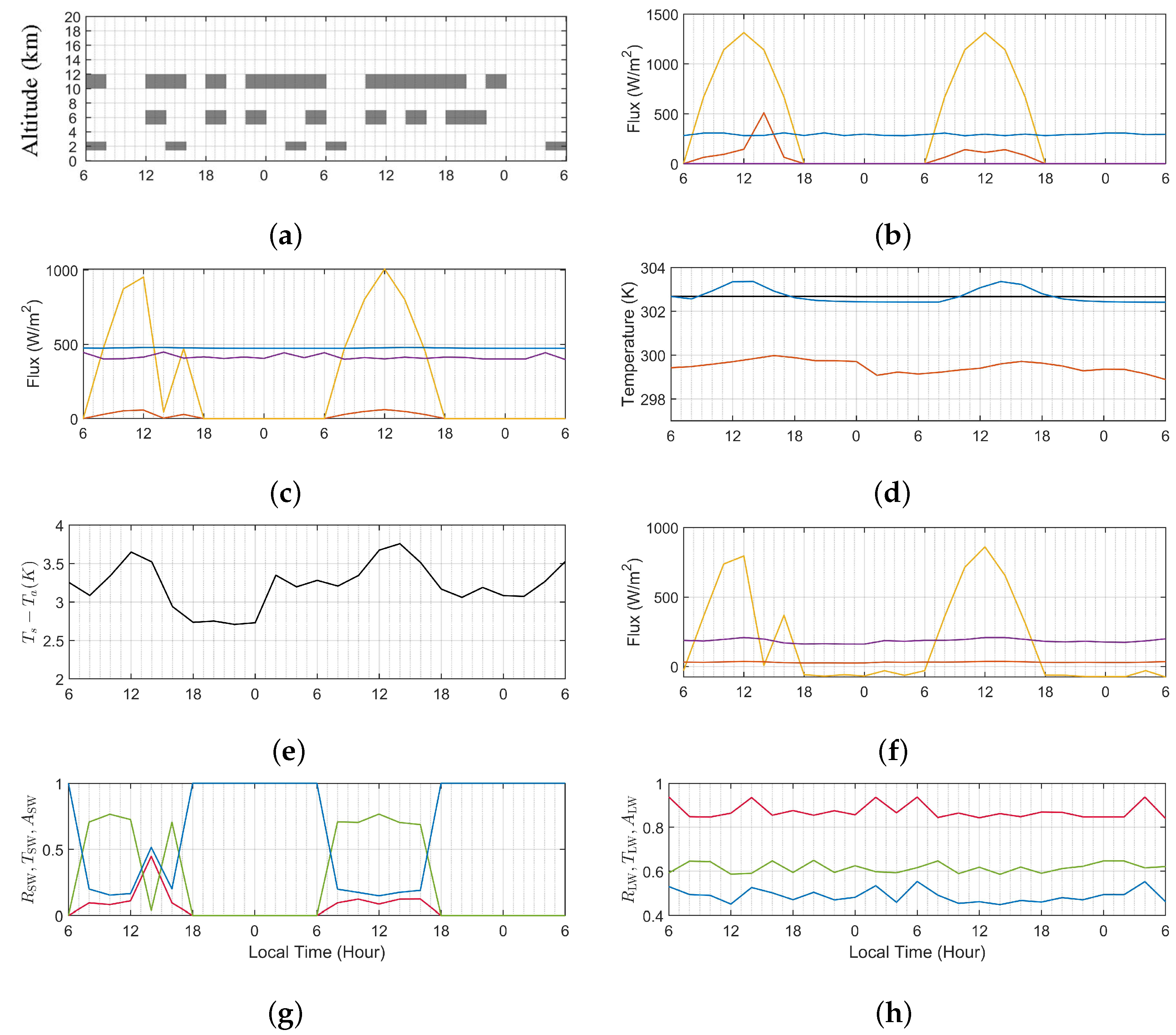
In summary, we conjecture that the cloud vertical structure change tends to raise T s in the post-hiatus period as more SW and LW energies are deposited near the air–sea interface than in the hiatus period.
Figure 10 shows the simulation results in the post-hiatus period, where Figure 10a–h are the counterparts of Figure 9a–h. The order of cloud types in the hiatus period shown in Figure 9a and that in the post-hiatus period shown in Figure 10a are arranged following the occurrence rates of cloud types listed in Table 6. The effects of cloud types on the R SW , T SW , A SW , R LW , T LW , and A LW shown in Figure 10g,h are consistent with their counterparts in Figure 9g,h. An obvious difference between the two periods is observed between Figure 9d and Figure 10d, that higher SST fdn in the post-hiatus lifts both T s and T a . Variation of wind speed in the post-hiatus is expected to affect the heat fluxes H and L e in Figure 10f, hence the temperature near the air–sea surface. However, its effect is not obvious from the simulation results over just two days.
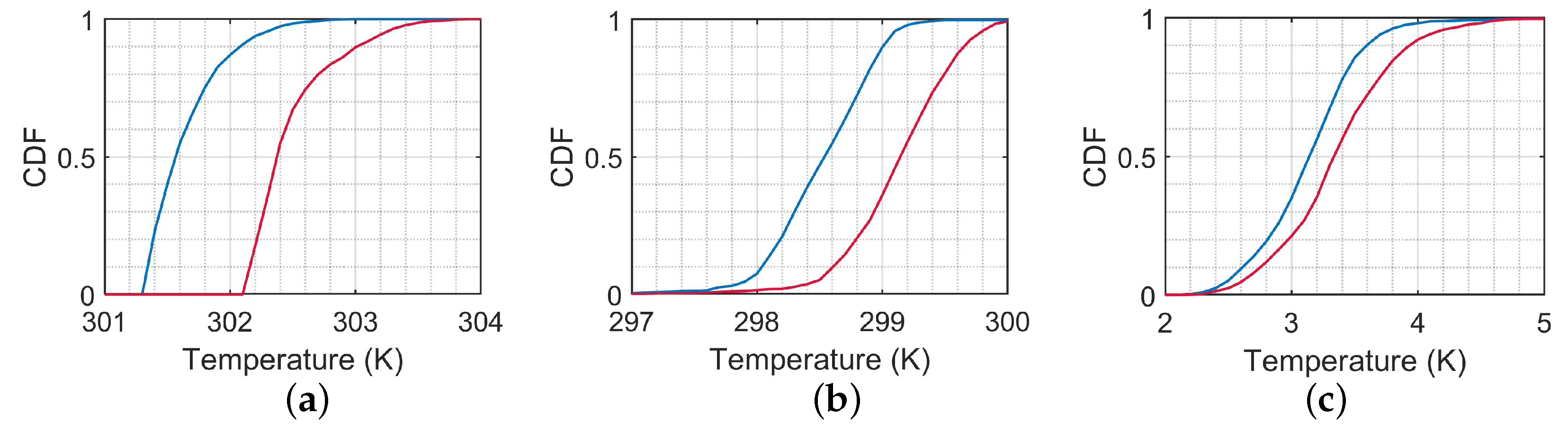
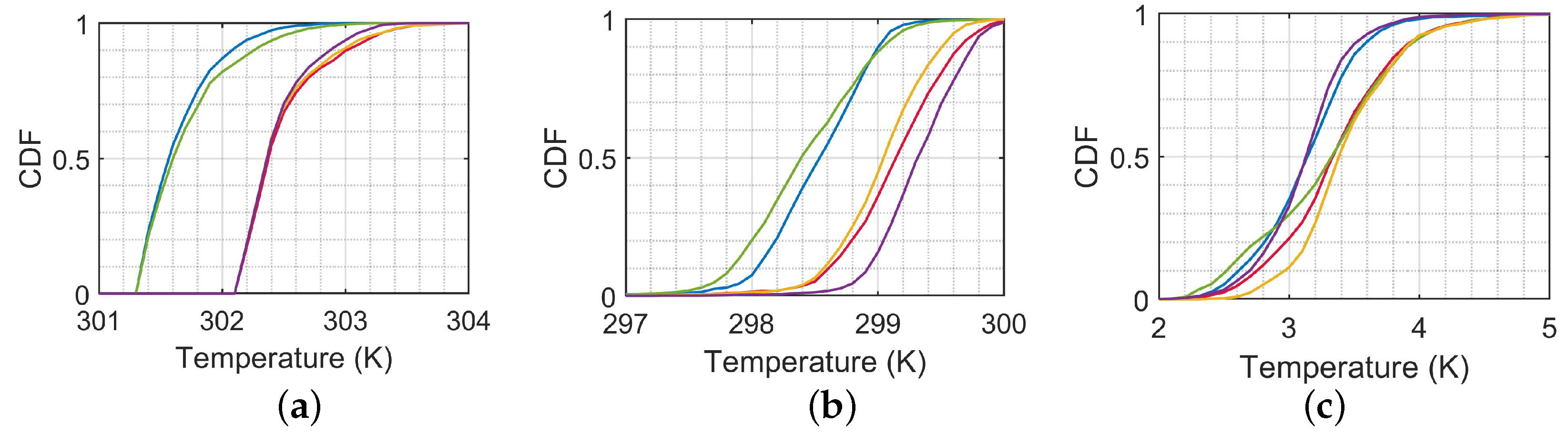
To observe the long-term effects of these three factors, the simulations of diurnal variation are run over a sufficient number of days. The simulated time sequences of T s and T a are analyzed statistically to gain more underlying information.
Figure 11 shows the cumulative distributions of T s , T a and T d = T s T a , respectively. The medians of T s and T a in the post-hiatus period are higher than their counterparts in the hiatus period by about 0.8 K and 0.6 K, respectively, leading to a difference of 0.2 K in the median of T d . More comparisons in subsequent cases will further manifest the relative significance of the three probable factors, SST fdn , F c and v a 10 .

5.2. Effects of Swapping Probable Factors

Table 8 lists the simulation cases designed by permutating the three probable factors with features listed in Table 7, where h and p indicate the factor is allocated from the hiatus and the post-hiatus period, respectively.
Denote the benchmark cases in the hiatus and post-hiatus periods presented in the last subsection as cases A and B, respectively. To distinguish the impact of these three factors listed in Table 7 upon the temperature change, cases C, D and E are fabricated, each having one (two) factor different from those in case A (case B). Cases F, G and H are fabricated, each having two (one) factors different from those in case A (case B).
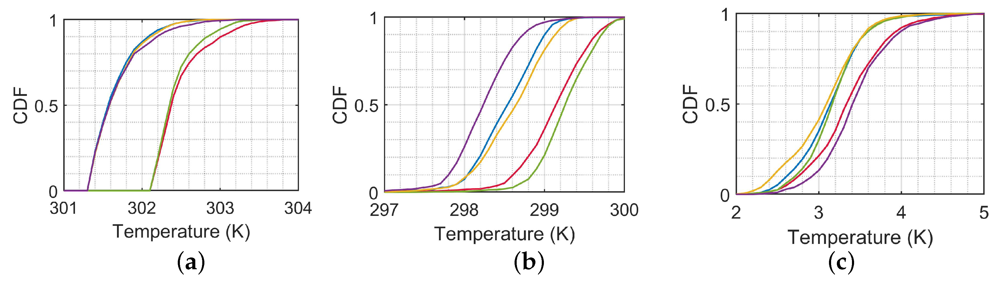
Figure 12 shows the CDFs of temperature near the air–sea interface in cases A, B, C, D and E, respectively. Figure 12a shows the CDFs of T s . Since T s is constrained by SST fdn , all the CDFs of T s have steeper slope (hence higher probability) near SST fdn . The CDFs of cases C, D and E shift right to that of case A, indicating T s is raised by swapping each probable factor with its counterpart in the post-hiatus period. The CDFs of cases B and C are separated from those of cases A, D and E, mainly due to the dominant influence of SST fdn over F c and v a 10 .
Figure 12b shows the CDFs of T a , which spread over a wider range than their counterparts of T s , attributed to lower heat capacity of air than water. The CDFs of cases C and D lean towards right compared with case A, indicating T a is raised by swapping SST fdn and F c , respectively. The CDF of case E leans towards left from that of case A, indicating T a drops due to lower v a 10 in the post-hiatus period.
Figure 12c shows the CDFs of T d . Since T a varies over a wider range than T s , the CDFs of T d are affected more by the variation of T a than T s . The CDFs of cases B and E are separated from those of cases A, C and D, especially near high T d .
Figure 13 shows the CDFs of temperature near the air–sea interface in cases A, B, F, G and H, respectively. The CDFs in Figure 13a,b are separated into one group of cases A and F, and another group of cases B, G and H, determined by SST fdn . The CDFs of cases F, G and H in Figure 13a lean towards the right compared with case A, indicating that T s is raised by three possible combinations of swapping two factors. In Figure 13b, lower T a median of case F compared with case A and higher T a median of cases G and H indicate the influence of SST fdn on the variation in T a . In Figure 13c, the CDFs of cases A and H are separated from those of cases B, F and G, especially near high T d .
An expedient analysis on the mean and median temperatures can provide some clues regarding the impacts of the three probable factors. Table 9 lists the median (med) and mean (avg) values of T s , T a and T d , respectively, for all eight cases presented in Figure 12 and Figure 13.
Table 10 lists the difference in temperatures of all the cases in Table 9 from their counterparts in the benchmark case A. The difference between the two benchmark cases (B–A) characterizes the transition from hiatus period to post-hiatus period.
Table 11 is similar to Table 10, except case B is used as benchmark. Next, we will scrutinize Table 10 and Table 11 to review the effects of different probable factors on T s , T a and T d , respectively.

5.3. Review on T s

Begin with T s . Table 10, case (B–A) lists the change from the hiatus period to the post-hiatus period, featuring higher SST fdn , different F c and lower v a 10 , as specified in Table 7 and Table 8. It is observed that T s , med and T s , avg increase by 0.803 K and 0.836 K, respectively. From a physical perspective, the increase in SST fdn raises T s , the lower occurrence rate of LC allows more SW flux to reach the surface, while the higher occurrence rate of HC and MC keeps more LW flux close to the surface, and lower v a 10 slows the transfer of heat from ocean to the air. The changes of all three factors tend to raise T s . The effect of each factor on raising T s can be examined in cases (C–A), (D–A) and (E–A), respectively, and the combined effects of two factors can be examined in cases (F–A), (G–A) and (H–A), respectively.
The increment of T s in case (B–A) is attributed unevenly to the three factors. Case (C–A) shows higher SST fdn contributes 0.779 K (0.779 K) to the median (mean), Case (D–A) shows different F c contributes 0.016 K (0.015 K) to the median (mean), and case (E–A) shows lower v a 10 contributes 0.012 K (0.037 K) to the median (mean).
The combined effect of two factors is not a direct sum of effects from the constituent factors. Case (F–A) shows different F c and lower v a 10 contribute 0.031 K (0.059 K) to T s , med ( T s , avg ), which is larger than the sum of their counterparts in cases (D–A) and (E–A). Case (G–A) shows higher SST fdn and lower v a 10 contribute 0.790 K (0.819 K) to T s , med ( T s , avg ), which is smaller (larger) than the sum of their counterparts in cases (C–A) and (E–A). Case (H–A) shows higher SST fdn and different F c contribute 0.790 K (0.794 K) to T s , med ( T s , avg ), which is smaller than (equal to) the sum of their counterparts in cases (C–A) and (D–A).
Similarly, Table 11 lists the difference of T s , med and T s , avg from case B. The effects of single factors on T s , med and T s , avg are shown in cases (F–B), (G–B), and (H–B), respectively. Case (F–B) shows lower SST fdn contributes 0.772 K ( 0.777 K) to T s , med ( T s , avg ), case (G–B) shows different F c contributes 0.013 K ( 0.017 K) to T s , med ( T s , avg ), and case (H–B) shows higher v a 10 contributes 0.013 K ( 0.042 K) to T s , med ( T s , avg ). These entries are consistent in terms of magnitude, with the entries of cases (C–A), (D–A) and (E–A), respectively, in Table 10, but with reversed signs.
Cases (C–B), (D–B), and (E–B) in Table 11 show the combined effects of two factors on T s , med and T s , avg . These entries are consistent with their counterparts of cases (F–A), (G–A) and (H–A), respectively, in Table 10. Case (D–B) and case (E–B) show large variation on T s , med and T s , avg , under the effects of lower SST fdn . Case (C–B) shows much smaller variation on T s , med and T s , avg , without the effect of lower SST fdn .
In summary, each of the three factors tends to raise T s , with SST fdn being the dominant factor. The combined effect of two factors is different from the sum of effects from the constituent factors. This conclusion is verified in Table 10 and Table 11 with the benchmarks of case A and case B, respectively.

5.4. Review on T a

Next, T a will be reviewed. The simulation results show that T a , med and T a , avg are lower than their counterparts T s , med and T s , avg in all the cases by about 3 K. This implies that heat fluxes H and L e are steadily released from ocean to the atmosphere via the air–sea interface, day and night.
Table 10, case (B–A) shows that T a , med and T a , avg in the post-hiatus period are higher than their counterparts in the hiatus period by 0.599 K and 0.615 K, respectively. The increments of T a , med and T a , avg are less than their counterparts in T s by about 0.2 K. From the physical point of view, higher SST fdn and different F c in the post-hiatus period tend to raise T a by retaining more heat energy in the atmospheric boundary layer, while lower v a 10 slows down the heat exchange in terms of H and L e , entering the air at the air–sea interface, tending to pull down T a .
Case (C–A) shows higher SST fdn contributes 0.722 K (0.751 K) to T a , med ( T a , avg ), case (D–A) shows different F c contributes 0.105 K (0.091 K) to T a , med ( T a , avg ), and case (E–A) shows lower v a 10 contributes 0.298 K ( 0.270 K) to T a , med ( T a , avg ).
Case (C–A) in Table 10 shows higher SST fdn raises T s by about 0.78 K, larger than 0.72-0.75 K of T a . The excess heat absorbed by the ocean during daytime is released to the air during night. Hence, the increment of T s is related to the increment of T a via heat exchange at the air–sea interface. Cases (D–A) and (E–A) in Table 10 show that different F c and lower v a 10 have stronger effect on T a than on T s . In other words, T a is more sensitive to the changes of F c or v a 10 , due to smaller heat capacity of air than water.
Next, combined effects of two factors on T a are reviewed. Case (H–A) shows the combined effects of higher SST fdn and different F c , contribute 0.778 K (0.807 K) to T a , med ( T a , avg ). Case (G–A) shows that higher SST fdn is partly offset by lower v a 10 , thus the increment of T a is smaller than that in case (C–A). Similarly, case (F–A) shows that different F c is partly offset by lower v a 10 , thus the increment of T a is smaller than that in case (D–A).
The T a entries in Table 11 are consistent with their counterparts in Table 10. Case (F–B) shows lower SST fdn changes T a , med ( T a , avg ) by 0.741 K ( 0.714 K). Case (G–B) shows different F c changes T a , med ( T a , avg ) by 0.092 K ( 0.099 K). Case (H–B) shows higher v a 10 changes T a , med ( T a , avg ) by 0.179 K (0.192 K). The impact of higher v a 10 is opposite to that of lower SST fdn or different F c . Hence, the combined effect of lower SST fdn and different F c , shown in case (E–B), has the largest impact of 0.897 K ( 0.885 K) on T a , med ( T a , avg ). The effects of the two other combinations, shown in cases (C–B) and (D–B), are relatively smaller since higher v a 10 tends to offset the effect of different F c and lower SST fdn , respectively.
In summary, the changes in T a by swapping the three factors are less regular than those of T s . Higher SST fdn and different F c in the post-hiatus period tend to raise T a , and lower v a 10 tends to pull down T a . The SST fdn still plays the dominant role in affecting T a , and is partly offset by the cooling effect of lower v a 10 on T a . The results in Table 10 are consistent with those in Table 11.

5.5. Review on T d

Finally, we will review the temperature difference, T d = T s T a , which determines the heat exchange across the air–sea interface explicitly via the sensible heat flux H and the latent heat flux L e . Case (B–A) in Table 10 shows that T d , med and T d , avg increase during the post-hiatus period.
The signs of T d , med and T d , avg in cases (C–A), (D–A), and (E–A) suggest that the effects of the three factors on T d are nonuniform, as in T a . Case (E–A) shows that a lower v a 10 has a relatively large impact of 0.267 K (0.307 K) on T d , med ( T d , avg ), because a lower v a 10 tends to raise T s and decrease T a . The increase in T d partly compensates for the effect of lower v a 10 on H and L e . The signs of T d , med and T d , avg in case (C–A) are opposite to those in case (D–A). Case (C–A) shows higher SST fdn tends to raise T s more than T a , leading to larger T d . On the other hand, case (D–A) shows different F c raises T s less than T a , leading to negative T d .
Case (G–A) shows the combined effects of higher SST fdn and lower v a 10 contribute 0.244 K (0.302 K) to T d , med ( T d , avg ). The other two combinations in cases (F–A) and (H–A) have weaker impact on T d than in the case (G–A), because different F c has opposite effect, as shown in case (D–A), to higher SST fdn or lower v a 10 , hence their effects offset with each other.
Case (H–B) in Table 11 shows higher v a 10 changes T d , med ( T d , avg ) by 0.200 K ( 0.234 K). The changes of T d in cases (F–B) and (G–B) are of opposite signs and smaller magnitude than their counterparts in (H–B).
In summary, the effects of three factors on T d are nonuniform, similar to T a . Lower v a 10 and higher SST fdn in the post-hiatus period tend to raise T d , and different F c tends to reduce it. The factor of SST fdn has a weaker impact on T d than on T s and T a . Instead, v a 10 becomes the dominant factor on T d , via affecting H and L e .

5.6. Summary on Simulation Results

In this section, two benchmark cases A and B are prepared to characterize the hiatus and post-hiatus periods, respectively, cases C, D and E are prepared to have one factor different from case A and two factors different from case B, cases F, G and H are prepared to have two factors different from case A and one factor different from case B. By scrutinizing the difference in simulation results with benchmark cases A and B, respectively, the effects of the three probable factors on T s , T a and T d are verified.
Higher SST fdn , different F c or lower v a 10 in the post-hiatus period tends to raise T s . Higher SST fdn and different F c tend to raise T a , while lower v a 10 tends to reduce it. Lower v a 10 or higher SST fdn tends to raise T d , and different F c tends to reduce it. SST fdn dominates the changes of T s and T a , while v a 10 dominates the change of T d .

5.7. Highlights of Contributions in This Work

The contributions of this work are summarized as follows.
  • We propose a modified one-dimensional radiative–convective model (1D-RCM) to simulate the diurnal pattern of temperature profile in a local region, incorporating convective adjustment, heat exchange with the ocean, absorption by greenhouse gases, and scattering by clouds.
  • We verify that the variation in cloud radiative effect (CRE) at the top of atmosphere (TOA) in the tropical western Pacific region after the end of recent hiatus is correlated with the variation in cloud vertical structure (CVS) thereof.
  • We propose an approach to study the long-term effect of CVS variation on the near-surface temperatures ( T s and T a ) by applying statistical analysis on their simulated short-term diurnal variations.
  • The results indicate that the variations in CVS, sea-surface temperature (SST) and wind speed have a positive effect on T s , but diverse effects on T a and T s T a .
  • The variation in near-surface temperatures suggests an acceleration of SST warming in the tropical western Pacific region.

5.8. Retrospect and Expectation

The major venture and payoff in this work is to predict the long-term climate-like trend of near-surface temperatures via simulating their short-term diurnal variation, followed by statistical analysis. Conventionally, long-term predictions were made by applying statistical techniques on measurement data or simulation results from complex climate models over a substantial period of time. Complex climate models may incorporate diverse mechanisms and become sensitive to input fluctuations. In this work, the diurnal patterns are simulated by developing a modified 1D-RCM, which incorporates the fundamental mechanisms and is less sensitive to input fluctuations. With the sprawling coverage of diverse sensor networks, more measurement data become available for monitoring the diurnal patterns of various parameters. The propose approach is easy to implement and modify to adapt to real-world measurement data.
The general concern regarding climate change is intuitively related to the long-term change in global temperature distribution. From a local perspective, the concern is related to the long-term temperature change near the surface at the same local time. A slight increase in long-term near-surface temperatures implies a huge amount of energy is deposited near ground or oceans, increasing the odds of weather calamities. Consider that a local station measures the near-surface temperatures continuously for decades. The recorded data can then be inspected for any long-term trends. If the station records the temperatures once daily, some of those long-term changes may still be observable, but are less convincing to explicate with relevant physical mechanisms. Using the diurnal pattern of temperature profile and relevant parameters, where available, to study the long-term trends will prove more robust than without such information.
Future technology will facilitate the acquisition of relevant parameters at a sufficiently high rate to establish creditable profiles of diurnal patterns. The proposed model and simulation approach can then be directly applied to real-world measurement data. Until then, simulations can still be applied to virtual data that manifest the features of the available data collected at limited temporal resolutions. In this work, the features focus on cloud vertical structure, foundation sea-surface temperature and wind speed. We try to simulate a set of diurnal patterns of these factors, based on their statistical attributes. These virtual profiles are not creditable for weather-like forecasts; however, the virtual profiles with different statistical attributes will manifest different features in the diurnal pattern of near-surface temperatures. The statistics on the diurnal temperature pattern can then be compared to speculate the effects of cloud vertical structure, foundation sea-surface temperature, and wind speed, respectively. In addition, the diurnal temperature pattern provides a vast array of speculative possible factors that may exacerbate climate change.

6. Conclusions

We find a correlation among foundation sea-surface temperature (SST fdn ), wind speed, ( v 10 a ) and cloud vertical structure (CVS) by comparing satellite observation data over a tropical western Pacific (TWP) region during the hiatus and post-hiatus periods transitioning in the spring of 2014. The variation in CVS is correlated with that of cloud radiative effects (CRE) at the top of atmosphere (TOA). A modified 1D radiative–convective model (RCM) considering heat exchange with the ocean has been developed to simulate the diurnal patterns of relevant variables to study the potential long-term effects of three probable factors (CVS, SST fdn and v 10 a ) on the near-surface temperatures T a in the air and T s at the sea surface, respectively.
The simulation results manifest a time delay between the peaks of T s and T a in their diurnal patterns. The rise in T s during the daytime and the drop in T a during night-time lead to two peaks in the diurnal pattern of temperature difference between them. Separate and combined effects of these three factors on T s and T a in the hiatus and post-hiatus periods are verified by statistical analysis on the simulation results over six cases fabricated with factors swapped between the two periods.
The SST fdn plays a dominant role in affecting both T s and T a in the tropic western Pacific region. All three factors tend to increase T s in the post-hiatus period. Higher SST fdn and different F c increase T a , while lower v 10 a tends to decrease T a .
The proposed model and the simulation results provide a clear picture to draw connections between the three probable factors to the near-surface temperatures, while excluding outlier weather conditions which may bias the general trend. The insights gained from this study may also be useful for planning future observation missions with data collected at finer spatial and temporal resolutions. The proposed approach can also be applied to study climate-related issues in other regions. Furthermore, the one-dimensional radiative–convective models (1D-RCMs) based on local atmospheric columns can be employed together to study the responses of wind field and cloud formations to variations in sea-surface temperature to predict more realistic and more complicated patterns.

Author Contributions

Conceptualization, C.-H.S. and J.-F.K.; methodology, C.-H.S. and J.-F.K.; software, C.-H.S.; validation, C.-H.S. and J.-F.K.; formal analysis, C.-H.S. and J.-F.K.; investigation, C.-H.S. and J.-F.K.; resources, J.-F.K.; data curation, C.-H.S.; Funding acquisition, J.-F.K.; writing—original draft preparation, C.-H.S.; writing—review and editing, J.-F.K.; visualization, C.-H.S. and J.-F.K.; supervision, J.-F.K.; project administration, J.-F.K. All authors have read and agreed to the published version of the manuscript.

Funding

This research was funded by the Ministry of Science and Technology, Taiwan, under contract MOST-109-2221-E-002-169.

Institutional Review Board Statement

Not applicable.

Informed Consent Statement

Not applicable.

Data Availability Statement

Not applicable.

Acknowledgments

This work was partly supported by a donation from the Pixart Imaging Inc. for promoting science and technology.

Conflicts of Interest

The authors declare no conflict of interest.

Abbreviations

The following abbreviations are used in this manuscript:
1D RCMone-dimensional radiative convective model
Acaltocumulus
Asaltostratus
CALIOPCloudSat and a cloud-aerosol lidar with orthogonal polarization
CALIPSOcloud-aerosol lidar and infrared pathfinder satellite observations
CDFcumulative distributions function
Cicirrus
CLclear-sky
CPRcloud-profiling radar
CREcloud radiative effect
Cucumulus
CVScloud vertical structure
DCdeep convective
ENSOEl Ni n ˜ o southern oscillation
ERSSTextended reconstructed SST
GHCNglobal historical climatology network
GISTEMPv4Goddard Institute for Space Studies surface temperature product version 4
GMSTglobal mean surface temperature
HChigh cloud
IPCCIntergovernmental Panel on Climate Change
IPOinterdecadal Pacific oscillation
IWCice water content
LClow cloud
LTlocal time
LTElocal thermodynamic equilibrium
LWlongwave
LWCliquid water content
MABLmarine atmospheric boundary layer
MCmiddle cloud
MLmulti-layered cloud
Nsnimbostratus
OPACoptical properties of aerosols and clouds package
PDOPacific decadal oscillation
RCEMIP      radiative convective equilibrium model intercomparison project
ROIregion of interest
Scstratocumulus
SLsingle-layered cloud
SSTsea-surface temperature
Ststratus
SWshortwave
TOAtop of atmosphere
TPITripole index
TTLtropical tropospheric layer
TWPtropical western Pacific

Appendix A. Physical Models

Appendix A.1. Radiative Transfer in Atmosphere

The atmosphere below 60–70 km roughly reaches local thermodynamic equilibrium (LTE) [9], and can be modeled as a stack of homogeneous planar layers piled up in z direction. In each planar layer, the upward radiance I (in z ^ direction) and the downward radiance I (in z ^ direction) follow the radiative transfer equations
μ d I ( τ ; μ , ϕ ) d τ = I ( τ ; μ , ϕ ) G ( τ ; μ , ϕ )
where 0 < μ ≤ 1, and τ is the optical depth [9]. The source functions G in (A1) and G in (A2) are composed of an emission part and a scattering part [9].
Figure A1 shows the schematic of a two-layered model, bounded by free space in regions (0) and (3) [9]. An intensity I ( μ 0 , ϕ 0 ) is incident from layer (0). The local reflection and transmission functions in layers (1) and (2) are ( R 1 , T ˜ 1 ) and ( R 2 , T ˜ 2 ), respectively. A superscript of asterisk means incidence from below. A multiple-scattering event in a layer can be decomposed into multiple single-scattering events, given by the product of corresponding local reflection/transmission functions. A multilayered model of atmosphere can be reduced to a two-layered model by applying the adding method recursively [9].
Figure A1. Two-layered model characterized with local reflections, local transmissions, combined reflections and combined transmissions [9].
Atmosphere 13 02130 g0a1
Define flux density as the sum of intensities over all upward or downward directions, respectively, as
J = 0 2 π 0 1 I ( μ , ϕ ) μ d μ d ϕ , J = 0 2 π 0 1 I ( μ , ϕ ) μ d μ d ϕ
which drives the heating rate T / t according to
T t = 1 ρ c p ( J J ) z
where ρ is the air density, c p = 1004 (m 2 /s 2 /K) is the specific heat of air under constant pressure.
The fluxes are computed by solving (A1)–(A3), in conjunction with the adding method. The evolution of temperature profile is then computed by solving (A4).

Appendix A.2. Convective Adjustment

Different convective adjustments have been proposed, with different lapse rate, fix or flexible surface temperature, to model the convection mechanism near surface [21,22,23,24]. In this work, we incorporate a convective adjustment based on the principle of energy conservation [22,24]. The temperature profile T ( s ) ( p ) at time step s and pressure level p is first updated as [9]
T ( p ) = T ( s ) ( p ) + Δ t T ( s ) ( p ) t
where T ( s ) ( p ) / t is driven by the radiative fluxes in (A4) and other heat fluxes from the oceans. Then, a convective adjustment [24]
Δ T c ( p ) = T ( s + 1 ) ( p ) T ( p )
is added to T ( p ) to attain a temperature profile T ( s + 1 ) ( p ) for the next time step as
T ( s + 1 ) ( p ) = T a ( s + 1 ) p p s γ p d p , p p c T ( p ) p < p c
where p s is the pressure (hPa) at the air–sea interface, T a ( s + 1 ) = T ( s + 1 ) ( p s ) is the air temperature just above the air–sea interface, and p c is the pressure (hPa) at the convection top, satisfying
T a ( s + 1 ) p p s γ p d p < T ( p ) , p < p c
γ p (K/pa) is the saturated isentropic lapse rate [24].
In an atmospheric layer with temperature T (K) and thickness d z (m), the change of its internal energy, d E c (J/m 2 ), associated with temperature change Δ T c (K) in (A5) due to convection is given by [22,24]
d E c = ρ c p Δ T c d z = c p g Δ T c d p
where ρ is the air density (kg/m 3 ).
The energy conservation principle implies that the change of total internal energy in the atmosphere is zero, with energy redistribution by convection, namely,
c p g 0 p s Δ T c ( p ) d p = 0
where Δ T c ( p ) is computed with (A5), T ( s + 1 ) ( p ) is computed with (A6), and T a ( s + 1 ) is iterated until (A7) is satisfied.

Appendix A.3. Heat Exchange with Ocean

Figure A2 shows the vertical profile of atmosphere coupling with ocean, where the top of atmosphere (TOA) is located at z toa , the air–sea interface is located at z = 0 , and the layer index is counted from below the TOA towards the air–sea interface.
Figure A2. Vertical profile of atmosphere coupling with ocean.
Atmosphere 13 02130 g0a2
The energy exchanges without convection in atmospheric layer ( i ) , with 1 i < i tc , where layer ( i tc ) is the topmost layer that involves convection. Black arrows and gray arrows indicate inflow energy and outflow energy, respectively, across layer interfaces. The change of internal energy Δ E i (J/m 2 ) over Δ t (s) in layer ( i ) is given by
Δ E i = Δ F i , 1 i < i tc
with
Δ F i = Δ t [ R ( z i + 1 ) R ( z i ) ]
where the net upward radiative flux R ( z ) (W/m 2 ) is the sum of the net upward shortwave flux J SW (W/m 2 ) and the net upward longwave flux J LW (W/m 2 ), namely,
R ( z ) = J SW ( z ) + J LW ( z ) = [ J SW ( z ) J SW ( z ) ] + [ J LW ( z ) J LW ( z ) ] , z 0
The energy exchanges with convection in atmospheric layer ( i ) , with i tc i < N a . The change of internal energy Δ E i (J/m 2 ) is given by
Δ E i = Δ F i + Δ E c i , i tc i < N a
with
Δ E c i = E c ( z i + 1 ) E c ( z i ) , i ct i N a
the net energy inflow due to convection, which can be given in terms of temperature as
Δ E c i = ρ i c p Δ z i Δ T c i , i ct i N a
where ρ i (kg/m 3 ) is the air density in layer ( i ) , Δ z i = z i z i + 1 (m) is the layer thickness and Δ T c i (K) is the change of T i (K) due to convection.
The net energy flux in layer ( N a ) is
Δ E N a = Δ F N a + Δ E c N a + H Δ t + L e Δ t
where H (W/m 2 ) and L e (W/m 2 ) are sensible heat flux and latent heat flux, respectively,
Δ E c N a = ρ N a c p Δ z N a Δ T c N a
is the net energy inflow due to convection, and Δ T c N a is given by (A5).
The sensible heat flux H and the latent heat flux L e in (A14) released from the air–sea interface are given by [59]
H = c s c p ρ a v a 10 ( T s b T a 10 )
L e = c L v ρ a v a 10 ( q s q a )
where ρ a (kg/m 3 ) is the air density at the air–sea interface, L v = 2.5 × 10 6 (J/kg) is the latent heat of vaporization, T s b ( ° C) is the sea-surface temperature, T a 10 ( ° C) and v a 10 (m/s) are the air temperature and wind speed, respectively, 10 m above mean sea level. The dimensionless coefficients c s and c are the sensible heat-flux coefficient and latent heat-flux coefficient, respectively, [59]. The variables ρ a , q a and q s in (A16) and (A17) are given in [59].
The variation of temperature in atmospheric layer ( i ) can therefore be derived from E i , respectively, from (A8), (A11) and (A14) as
T i t = 1 ρ i c p Δ z i E i t , 1 i N a
The energy exchange in ocean layer ( N a + 1 ) is given by
Δ E N a + 1 = Δ t R s H Δ t L e Δ t
where H and L e are given in (A16) and (A17), respectively, and R s is the net radiative flux entering the bulk ocean, which is approximated as [44]
R s = 1.2 [ J SW ( z N a + 1 ) J SW ( z N a + 1 ) ] f w + [ J LW ( z N a + 1 ) J LW ( z N a + 1 ) ]
with f w to account for the absorption of solar irradiance by water [44].

References

  1. Masson-Delmotte, V.; Zhai, P.; Pörtner, H.-O.; Roberts, D.; Skea, J.; Shukla, P.R. (Eds.) Annex I: Glossary in Global Warming of 1.5 °C, An IPCC Special Report on the Impacts of Global Warming of 1.5 °C above Pre-Industrial Levels and Related Global Greenhouse Gas Emission Pathways, in the Context of Strengthening the Global Response to the Threat of Climate Change, Sustainable Development, and Efforts to Eradicate Poverty; Cambridge University Press: Cambridge, UK; New York, NY, USA, 2018; pp. 541–562. [Google Scholar] [CrossRef]
  2. Stocker, T.F.; Qin, D.; Plattner, G.-K.; Tignor, M.; Allen, S.K.; Boschung, J. (Eds.) Technical Summary. In Climate Change 2013—The Physical Science Basis. Contribution of Working Group I to the Fifth Assessment Report of the Intergovernmental Panel on Climate Change; Cambridge University Press: Cambridge, UK; New York, NY, USA, 2013; pp. 31–116. [Google Scholar] [CrossRef]
  3. Douville, H.; Voldoire, A.; Geoffroy, O. The recent global warming hiatus: What is the role of Pacific variability? Geophys. Res. Lett. 2015, 42, 880–888. [Google Scholar] [CrossRef]
  4. Xie, S.P.; Kosaka, Y. What caused the global surface warming hiatus of 1998–2013? Curr. Clim. Change Rep. 2017, 3, 128–140. [Google Scholar] [CrossRef]
  5. Hansen, J.; Ruedy, R.; Sato, M.; Lo, K. Global surface temperature change. Rev. Geophys. 2010, 48, RG4004. [Google Scholar] [CrossRef] [Green Version]
  6. England, M.H.; McGregor, S.; Spence, P.; Meehl, G.A.; Timmermann, A.; Cai, W.; Gupta, A.S.; McPhaden, M.J.; Purich, A.; Santoso, A. Recent intensification of wind-driven circulation in the Pacific and the ongoing warming hiatus. Nat. Clim. Chang. 2014, 4, 222–227. [Google Scholar] [CrossRef] [Green Version]
  7. Loeb, N.G.; Thorsen, T.J.; Norris, J.R.; Wang, H.; Su, W. Changes in Earth’s Energy Budget during and after the “Pause” in Global Warming: An Observational Perspective. Climate 2018, 6, 62. [Google Scholar] [CrossRef] [Green Version]
  8. L’Ecuyer, T.S.; Hang, Y.; Matus, A.V.; Wang, Z. Reassessing the effect of cloud type on earth’s energy balance in the age of active spaceborne observations, Part I: Top of atmosphere and surface. J. Clim. 2019, 32, 6197–6217. [Google Scholar] [CrossRef] [Green Version]
  9. Liou, K.N. An Introduction to Atmospheric Radiation, 2nd ed.; Academic Press: New York, NY, USA, 2002. [Google Scholar]
  10. Hang, Y.; L’Ecuyer, T.S.; Henderson, D.S.; Matus, A.V.; Wang, Z. Reassessing the effect of cloud type on earth’s energy balance in the age of active spaceborne observations, Part II: Atmospheric heating. J. Clim. 2019, 32, 6219–6236. [Google Scholar] [CrossRef]
  11. Johansson, E.; Devasthale, A.; Ekman, A.M.L.; Tjernstrom, M.; L’Ecuyer, T. How does cloud overlap affect the radiative heating in the tropical upper troposphere/lower stratosphere? Geophys. Res. Lett. 2019, 46, 5623–5631. [Google Scholar] [CrossRef]
  12. Mao, K.; Yuan, Z.; Zuo, Z.; Xu, T.; Shen, X.; Gao, C. Changes in Global Cloud Cover Based on Remote Sensing Data from 2003 to 2012. Chin. Geogr. Sci. 2019, 29, 306–315. [Google Scholar] [CrossRef] [Green Version]
  13. Brient, F.; Bony, S. Interpretation of the positive low-cloud feedback predicted by a climate model under global warming. Clim. Dyn. 2012, 40, 2415–2431. [Google Scholar] [CrossRef] [Green Version]
  14. Kamae, Y.; Ogura, T.; Watanabe, M.; Xie, S.-P.; Ueda, H. Robust cloud feedback over tropical land in a warming climate. J. Geophys. Res. Atmos. 2016, 121, 2593–2609. [Google Scholar] [CrossRef] [Green Version]
  15. Morrison, A.L.; Kay, J.E.; Frey, W.R.; Chepfer, H.; Guzman, R. Cloud Response to Arctic Sea Ice Loss and Implications for Future Feedback in the CESM1 Climate Model. J. Geophys. Res. Atmos. 2019, 124, 1003–1020. [Google Scholar] [CrossRef]
  16. Zhou, C.; Zelinka, M.D.; Klein, S.A. Analyzing the dependence of global cloud feedback on the spatial pattern of sea surface temperature change with a G reen’s function approach. J. Adv. Model. Earth Syst. 2017, 9, 2174–2189. [Google Scholar] [CrossRef] [Green Version]
  17. Ceppi, P.; Nowack, P. Observational evidence that cloud feedback amplifies global warming. Proc. Natl. Acad. Sci. USA 2021, 118, e2026290118. [Google Scholar] [CrossRef]
  18. Chepfer, H.; Noel, V.; Winker, D.; Chiriaco, M. Where and when will we observe cloud changes due to climate warming? Geophys. Res. Lett. 2014, 41, 8387–8395. [Google Scholar] [CrossRef]
  19. Ohno, T.; Noda, A.T.; Seiki, T.; Satoh, M. Importance of Pressure Changes in High Cloud Area Feedback due to Global Warming. Geophys. Res. Lett. 2021, 48, e2021GL093646. [Google Scholar] [CrossRef]
  20. Wang, Z.; Ge, J.; Yan, J.; Li, W.; Yang, X.; Wang, M.; Hu, X. Interannual shift of tropical high cloud diurnal cycle under global warming. Clim. Dyn. 2022, 59, 3391–3400. [Google Scholar] [CrossRef]
  21. Fu, Q.; Smith, M.; Yang, Q. The Impact of Cloud Radiative Effects on the Tropical Tropopause Layer Temperatures. Atmosphere 2018, 9, 377. [Google Scholar] [CrossRef]
  22. Manabe, S.; Wetherald, R.T. Thermal equilibrium of the atmosphere with a given distribution of relative humidity. J. Atmos. Sci. 1967, 24, 241–259. [Google Scholar] [CrossRef]
  23. Thuburn, J.; Craig, G.C. On the temperature structure of the tropical substratosphere. J. Geophys. Res. Atmos. 2002, 107, ACL 10-1–ACL 10-10. [Google Scholar] [CrossRef]
  24. Kluft, L.; Dacie, S.; Buehler, S.A.; Schmidt, H.; Stevens, B. Re-Examining the First Climate Models: Climate Sensitivity of a Modern Radiative–Convective Equilibrium Model. J. Clim. 2019, 32, 8111–8125. [Google Scholar] [CrossRef] [Green Version]
  25. Dacie, S.; Kluft, L.; Schmidt, H.; Stevens, B.; Buehler, S.A.; Nowack, P.J.; Dietmüller, S.; Abraham, N.L.; Birner, T. A 1D RCE Study of Factors Affecting the Tropical Tropopause Layer and Surface Climate. J. Clim. 2019, 32, 6769–6782. [Google Scholar] [CrossRef] [Green Version]
  26. O’Neill, L.W.; Chelton, D.B.; Esbensen, S.K. Observations of SST-Induced Perturbations of the Wind Stress Field over the Southern Ocean on Seasonal Timescales. J. Clim. 2003, 16, 2340–2354. [Google Scholar] [CrossRef] [Green Version]
  27. Chelton, D.B.; Schlax, M.G.; Samelson, R.M. Summertime Coupling between Sea Surface Temperature and Wind Stress in the California Current System. J. Phys. Oceanogr. 2007, 37, 495–517. [Google Scholar] [CrossRef]
  28. O’Neill, L.W.; Chelton, D.B.; Esbensen, S.K. The Effects of SST-Induced Surface Wind Speed and Direction Gradients on Mid-latitude Surface Vorticity and Divergence. J. Clim. 2010, 23, 255–281. [Google Scholar] [CrossRef]
  29. Fallmann, J.; Lewis, H.; Castillo, J.M.; Arnold, A.; Ramsdale, S. Impact of sea surface temperature on stratiform cloud formation over the North Sea. Geophys. Res. Lett. 2017, 44, 4296–4303. [Google Scholar] [CrossRef]
  30. Ricchi, A.; Bonaldo, D.; Cioni, G.; Carniel, S.; Miglietta, M.M. Simulation of a flash-flood event over the Adriatic Sea with a high-resolution atmosphere–ocean–wave coupled system. Sci. Rep. 2021, 11, 9388. [Google Scholar] [CrossRef]
  31. GISTEMP Team. GISS Surface Temperature Analysis (GISTEMP), Version 4, NASA Goddard Institute for Space Studies. 2021. Available online: https://data.giss.nasa.gov/gistemp/ (accessed on 18 October 2021).
  32. Lenssen, N.J.L.; Schmidt, G.A.; Hansen, J.E.; Menne, M.J.; Persin, A.; Ruedy, R.; Zyss, D. Improvements in the GISTEMP Uncertainty Model. J. Geophys. Res. Atmos. 2019, 124, 6307–6326. [Google Scholar] [CrossRef]
  33. Huang, B.; Thorne, P.W.; Banzon, V.F.; Boyer, T.; Chepurin, G.; Lawrimore, J.H.; Menne, M.J.; Smith, T.M.; Vose, R.S.; Zhang, H.-M. NOAA Extended Reconstructed Sea Surface Temperature (ERSST), Version 5. [ersst.v5]. NOAA Natl. Cent. Environ. Inf. 2017. [Google Scholar] [CrossRef]
  34. Pacific Decadal Oscillation. Available online: https://www.ncdc.noaa.gov/teleconnections/pdo/ (accessed on 14 December 2021).
  35. Mantua, N.J.; Hare, S.R. The Pacific decadal oscillation. J. Oceanogr. 2002, 58, 35–44. [Google Scholar] [CrossRef]
  36. Henley, B.J.; Gergis, J.; Karoly, D.J.; Power, S.; Kennedy, J.; Folland, C.K. A Tripole Index for the Interdecadal Pacific Oscillation. Clim. Dyn. 2015, 45, 3077–3090. [Google Scholar] [CrossRef]
  37. Loeb, N.G.; Doelling, D.R.; Wang, H.; Su, W.; Nguyen, C.; Corbett, J.G.; Liang, L.; Mitrescu, C.; Rose, F.G.; Kato, S. Clouds and the Earth’s Radiant Energy System (CERES) Energy Balanced and Filled (EBAF) Top-of-Atmosphere (TOA) Edition-4.0 Data Product. J. Clim. 2018, 31, 895–918. [Google Scholar] [CrossRef]
  38. Stephens, G.; Winker, D.; Pelon, J.; Trepte, C.; Vane, D.; Yuhas, C.; L’Ecuyer, T.; Lebsock, M. CloudSat and CALIPSO within the A-Train: Ten Years of Actively Observing the Earth System. Bull. Am. Meteorol. Soc. 2018, 99, 569–581. [Google Scholar] [CrossRef] [Green Version]
  39. Sassen, K.; Wang, Z.; Liu, D. Global distribution of cirrus clouds from CloudSat/cloud-aerosol lidar and infrared pathfinder satellite observations (CALIPSO) measurements. J. Geophys. Res. Atmos. 2008, 113, D00A12. [Google Scholar] [CrossRef]
  40. Sassen, K.; Wang, Z. Classifying clouds around the globe with the CloudSat radar: 1-year of results. Geophys. Res. Lett. 2008, 35, L04805. [Google Scholar] [CrossRef]
  41. Gao, S.; Cui, X.; Li, X. A modeling study of relation between cloud amount and SST over Western Tropical Pacific cloudy regions during TOGA COARE. Prog. Nat. Sci. 2009, 19, 187–193. [Google Scholar] [CrossRef]
  42. Cesana, G.; Del Genio, A.D.; Ackerman, A.S.; Kelley, M.; Elsaesser, G.; Fridlind, A.M.; Cheng, Y.; Yao, M.-S. Evaluating models’ response of tropical low clouds to SST forcings using CALIPSO observations. Atmos. Chem. Phys. 2019, 19, 2813–2832. [Google Scholar] [CrossRef] [Green Version]
  43. Hersbach, H.; Bell, B.; Berrisford, P.; Biavati, G.; Horanyi, A.; Mun˜oz-Sabater, J. ERA5 Monthly Averaged Data on Single Levels from 1979 to Present. Copernicus Climate Change Service (C3S) Climate Data Store (CDS). 2019. Available online: https://cds.climate.copernicus.eu/cdsapp#!/dataset/10.24381/cds.f17050d7?tab=overview (accessed on 5 January 2022).
  44. Gentemann, C.; Minnett, P.J.; Ward, B. Profiles of ocean surface heating (POSH): A new model of upper ocean diurnal warming. J. Geophys. Res. 2009, 114, C07017. [Google Scholar] [CrossRef]
  45. Comstock, J.M.; Protat, A.; McFarlane, S.A.; Delanoë, J.; Deng, M. Assessment of uncertainty in cloud radiative effects and heating rates through retrieval algorithm differences: Analysis using 3 years of ARM data at Darwin, Australia. J. Geophys. Res. Atmos. 2013, 118, 4549–4571. [Google Scholar] [CrossRef]
  46. Comstock, J.; McFarlane, S. Atmospheric Radiation Measurement (ARM) User Facility, 1994, Updated Daily. Cloud Properties and Radiative Heating Rates Dataset for Nauru, Manus, and Darwin Sites. January 2008–February 2009, 0° 31′ 15.6″ S, 166° 54′ 57.6″ E: Central Facility, Nauru Island (TWP C2); ARM Data Center: Oak Ridge, TN, USA, 2017. [Google Scholar]
  47. Hess, M.; Koepke, P.; Schult, I. Optical Properties of Aerosols and Clouds: The Software Package OPAC. Bull. Am. Meteorol. Soc. 1998, 79, 831–844. [Google Scholar] [CrossRef]
  48. Wing, A.A.; Reed, K.A.; Satoh, M.; Stevens, B.; Bony, S.; Ohno, T. Radiative–convective equilibrium model intercomparison project. Geosci. Model Dev. 2018, 11, 793–813. [Google Scholar] [CrossRef] [Green Version]
  49. McLean, A.B.; Mitchell, C.E.J.; Swanston, D.M. Implementation of an efficient analytical approximation to the Voigt function for photoemission lineshape analysis. J. Electron. Spectrosc. Relat. Phenom. 1994, 69, 125–132. [Google Scholar] [CrossRef]
  50. Gordon, I.E.; Rothman, L.S.; Hill, C.; Kochanov, R.V.; Tan, Y.; Bernath, P.F.; Birk, M.; Boudon, V.; Campargue, A.; Chance, K.V.; et al. The HITRAN2016 molecular spectroscopic database. J. Quant. Spectrosc. Radiat. Transf. 2017, 203, 3–69. [Google Scholar] [CrossRef]
  51. Molina, L.T.; Molina, M.J. Absolute absorption cross sections of ozone in the 185- to 350-nm wavelength range. J. Geophys. Res. Atmos. 1986, 91, 14501–14508. [Google Scholar] [CrossRef]
  52. Mlawer, E.J.; Payne, V.H.; Moncet, J.-L.; Delamere, J.S.; Alvarado, M.J.; Tobin, D.C. Development and recent evaluation of the MT_CKD model of continuum absorption. Philos. Trans. R. Soc. A Math. Phys. Eng. Sci. 2012, 370, 2520–2556. [Google Scholar] [CrossRef] [Green Version]
  53. Li, M.; Liao, Z.; Coimbra, C.F. Spectral model for clear sky atmospheric longwave radiation. J. Quant. Spectrosc. Radiat. Transf. 2018, 209, 196–211. [Google Scholar] [CrossRef]
  54. Bucholtz, A. Rayleigh-scattering calculations for the terrestrial atmosphere. Appl. Opt. 1995, 34, 2765–2773. [Google Scholar] [CrossRef]
  55. Hu, Y.X.; Stamnes, K. An accurate parameterization of the radiative properties of water clouds suitable for use in climate models. J. Clim. 1993, 6, 728–742. [Google Scholar] [CrossRef]
  56. Fu, Q. An Accurate Parameterization of the Solar Radiative Properties of Cirrus Clouds for Climate Models. J. Clim. 1996, 9, 2058–2082. [Google Scholar] [CrossRef]
  57. Fu, Q.; Yang, P.; Sun, W.B. An Accurate Parameterization of the Infrared Radiative Properties of Cirrus Clouds for Climate Models. J. Clim. 1998, 11, 2223–2237. [Google Scholar] [CrossRef]
  58. Jin, Z.; Charlock, T.P.; Rutledge, K.; Stamnes, K.; Wang, Y. Analytical solution of radiative transfer in the coupled atmos-phere-ocean system with a rough surface. Appl. Opt. 2006, 45, 7443–7455. [Google Scholar] [CrossRef] [PubMed]
  59. Kara, A.B.; Rochford, P.A.; Hurlburt, H.E. Efficient and accurate bulk parameterizations of air–sea fluxes for use in general circulation models. J. Atmos. Ocean. Technol. 2000, 17, 1421–1438. [Google Scholar] [CrossRef]
Figure 1. Anomaly in global mean surface temperature (GMST) between 1920–2020 with respect to the average value between 1951–1980, ——: annual mean value [31], ——: annual mean value smoothed with LOWESS (locally weighted scatterplot smoothing) over five-year window [31], grey region: hiatus periods in 1943–1976 and 1998–2014.
Atmosphere 13 02130 g001
Figure 2. Pacific decadal oscillation (PDO) index (——) [34] and Tripole index (TPI) (——) of interdecadal Pacific oscillation (IPO) [36] in 1920–2020.
Atmosphere 13 02130 g002
Figure 3. Pacific decadal oscillation (PDO) index (——) [34] and Tripole index (TPI) (——) of interdecadal Pacific oscillation (IPO) [36] between 2006–2018.
Atmosphere 13 02130 g003
Figure 4. (a) Mean sea-surface temperature anomalies Δ SST d = Δ SST p Δ SST h (K) based on 1971–2000 climatology [33]. (b) Difference in cloud radiative effect, Δ CRE net (W/m 2 ), at TOA between hiatus period and post-hiatus period [37], (c) difference in shortwave (SW) cloud radiative effect, Δ CRE SW (W/m 2 ), at TOA between two periods [37], (d) difference in longwave (LW) cloud radiative effect, Δ CRE LW (W/m 2 ), at TOA between two periods [37]. Rectangle encloses the region of interest (ROI) in tropical western Pacific.
Atmosphere 13 02130 g004
Figure 5. Cloud types in CloudSat 2B-CLDCLASS-lidar product [40].
Atmosphere 13 02130 g005
Figure 6. Average sea-surface temperature at 6 AM local time, ——: hiatus period, ——: post-hiatus period [43].
Atmosphere 13 02130 g006
Figure 7. (a) Average wind speed during hiatus period, v a 10 , h (m/s) [43]. (b) Difference in average wind speed between post-hiatus and hiatus periods [43].
Atmosphere 13 02130 g007
Figure 8. Prototypes of cloud vertical structure specified in simulations, (a) HC, (b) MC, (c) LC, (d) HC + LC and (e) HC + MC.
Atmosphere 13 02130 g008
Figure 9. Simulation data over 48 h (d1h6–d3h6) in hiatus period, (a) cloud pattern, (b) flux density at TOA, ——: J SW , ——: J SW , ——: J LW , ——: J LW , (c) flux density at air–sea interface, (d) temperature at air–sea interface, ——: T s , ——: T a , ——: T fdn , (e) T s T a at air–sea interface, (f) radiative and heat fluxes at air–sea interface, ——: R surf , ——: H, ——: L e , (g) cloud effect on SW, ——: R SW , ——: T SW , ——: A SW , (h) cloud effect on LW, ——: R LW , ——: T LW , ——: A LW .
Atmosphere 13 02130 g009
Figure 10. Simulation data over 48 h (d1h6-d3h6) in post-hiatus period, (a) cloud pattern, (b) flux density at TOA, ——: J SW , ——: J SW , ——: J LW , ——: J LW , (c) flux density at air–sea interface, (d) temperature at air–sea interface, ——: T s , ——: T a , ——: T fdn , (e) T s T a at air–sea interface, (f) radiative and heat fluxes at air–sea interface, ——: R surf , ——: H, ——: L e , (g) cloud effect on SW, ——: R SW , ——: T SW , ——: A SW , (h) cloud effect on LW, ——: R LW , ——: T LW , ——: A LW .
Atmosphere 13 02130 g010
Figure 11. CDF of (a) T s , (b) T a , (c) T d , ——: hiatus period, ——: post-hiatus period.
Atmosphere 13 02130 g011
Figure 12. CDF of (a) T s , (b) T a , (c) T d , ——: case A, ——: case B, ——: case C, ——: case D, and ——: case E.
Atmosphere 13 02130 g012
Figure 13. CDF of (a) T s , (b) T a , (c) T s T a , ——: case A, ——: case B, ——: case F, ——: case G, and ——: case H.
Atmosphere 13 02130 g013
Table 1. Region of interest and time windows.
DomainDescriptionReference
TimeHiatus period (March 2006 to February 2014), post-hiatus period (March 2014 to February 2019)Figure 3
RegionRectangle with corners at ( ϕ lat , ϕ lon ) = ( 2 . 50 ° N, 165 ° E), ( 2 . 50 ° N, 170 ° W), ( 7 . 50 ° S, 170 ° W) and ( 7 . 50 ° S, 165 ° E)Figure 4
Table 2. Occurrence rate (%) of CVS features.
(a) Occurrence Rate (%) of Cloud Layer Number
Number0123456–10Total
F h 23.3841.9124.038.112.050.430.09100
Δ F 4.09 1.68 2.582.060.840.240.050
(b) Occurrence Rate (%) of Single-Layer Cloud Type
TypeCiAsAcStScCuNsD.C.Total
F h 20.981.871.620.011.4514.300.770.9141.91
Δ F 0.590.920.25 0.01 0.62 4.00 0.380.81 1.68
(c) Occurrence Rate (%) of Double-Layer Cloud Type in Hiatus Period
TypeCiAsAcStScCuNsD.C.Total
Ci5.8000000005.80
As1.520.030.01000001.56
Ac2.570.360.18000003.11
St0.0100000000.01
Sc1.170.080.1000.020.01001.38
Cu10.050.280.4300.100.270011.13
Ns0.550.020000000.57
D.C.0.4700000000.47
Total22.140.770.7200.120.280024.03
(d) Occurrence Rate (%) of Bottom Cloud Type in Double-Layer Cloud, with Ci as Top Cloud
TypeCiAsAcStScCuNsD.C.Total
F h 5.801.522.570.011.1710.050.550.4722.14
Δ F 0.900.681.03 0.01 0.17 0.72 0.240.292.24
Table 3. Regroup of cloud types for simulations in this study.
TypeFull NameDefinition
CLclear-skyno cloud
SLsingle-layer1 layer of cloud
MLmulti-layer2 or more layers of cloud
HChigh cloudCi and D.C. in Figure 5
MCmiddle cloudAs, Ac and Ns in Figure 5
LClow cloudCu, Sc and St in Figure 5
Table 4. Occurrence rate (%) of cloud types after regroup.
(a) Occurrence Rate (%) of Regrouped Sky Condition
TypeCLSLMLTotal
F h 23.3841.9134.71100
Δ F 4.09 1.68 5.770
(b) Occurrence Rate (%) of Regrouped Single-Layer Cloud
TypeLCMCHCTotal
F h 15.764.2621.8941.91
Δ F 4.63 1.551.40 1.68
(c) Occurrence Rate (%) of Bottom-Cloud Type in Regrouped Double-Layer Cloud, with Ci as Top Cloud
TypeLCMCHCMC or HCTotal
F h 11.234.646.2710.9122.14
Δ F −0.901.951.193.142.24
Table 5. Parameters of cloud types in simulations.
(a)
TypePhase z top (km) z bot (km) D ge ( μ m)IWC (g/m 3 )
HCice12 [45]10 [45]45 [45] 10 3 [45]
MCice7 [45]5 [45]90 [45] 10 2 [45]
(b)
TypePhase z top (km) z bot (km) r eff ( μ m)LWC (g/m 3 )
LCliquid2.5 [45]1.5 [45]12.68 [47]0.44 [47]
Table 6. Occurrence rate (%) of cloud type in simulations.
Type F h ( % ) F p ( % ) Δ F ( % )
CL23.3819.29 4.09
LC15.7611.13 4.63
MC4.265.811.55
HC21.8923.291.40
HC + LC17.6117.15 0.46
HC + MC17.1023.336.23
total1001000
Table 7. Trend of probable factors in the hiatus and post-hiatus periods.
FactorVariation between Two PeriodsReference
SST fdn Higher in post-hiatus ( Δ SST fdn > 0 )Figure 6
CVS ( F c )Post-hiatus features more cloudiness, more cloud layers and fewer low cloudsTable 6
v a 10 Lower in post-hiatus ( Δ v a 10 < 0 )Figure 7
Table 8. Simulation cases and allocated factors.
CaseABCDEFGH
SST fdn hpphhhpp
F c hphphphp
v a 10 hphhppph
Table 9. Statistics of T s , T a and T d in 8 cases.
Case T s , med T s , avg T a , med T a , avg T d , med T d , avg
A301.569301.646298.536298.5113.1403.135
B302.372302.482299.135299.1263.3293.356
C302.348302.425299.258299.2623.1583.164
D301.585301.661298.641298.6023.0953.059
E301.581301.683298.238298.2413.4073.442
F301.600301.705298.394298.4123.3213.292
G302.359302.465299.043299.0273.3843.437
H302.359302.440299.314299.3183.1293.122
Table 10. Difference of T s , T a and T d from case A.
Case T s , med T s , avg T a , med T a , avg T d , med T d , avg
B–A0.8030.8360.5990.6150.1890.221
C–A0.7790.7790.7220.7510.0180.029
D–A0.0160.0150.1050.091−0.045−0.076
E–A0.0120.037−0.298−0.2700.2670.307
F–A0.0310.059−0.142−0.0990.1810.157
G–A0.7900.8190.5070.5160.2440.302
H–A0.7900.7940.7780.807−0.011−0.013
Table 11. Difference of T s , T a and T d from case B.
Case T s , med T s , avg T a , med T a , avg T d , med T d , avg
A–B−0.803−0.836−0.599−0.615−0.189−0.221
C–B−0.024−0.0570.1230.136−0.171−0.192
D–B−0.787−0.821−0.494−0.524−0.234−0.297
E–B−0.791−0.799−0.897−0.8850.0780.086
F–B−0.772−0.777−0.741−0.714−0.008−0.064
G–B−0.013−0.017−0.092−0.0990.0550.081
H–B−0.013−0.0420.1790.192−0.200−0.234
Publisher’s Note: MDPI stays neutral with regard to jurisdictional claims in published maps and institutional affiliations.

