Influence of ENSO on Droughts and Vegetation in a High Mountain Equatorial Climate Basin

Abstract

Several studies have assessed droughts and vegetation considering climatic factors, particularly El Niño-Southern Oscillation (ENSO) at different latitudes. However, there are knowledge gaps in the tropical Andes, a region with high spatiotemporal climatic variability. This research analyzed the relationships between droughts, vegetation, and ENSO from 2001–2015. Meteorological drought was analyzed using the Standardized Precipitation Evapotranspiration Index (SPEI) for 1, 3 and 6 months. Normalized Difference Vegetation Index (NDVI) was used to evaluate vegetation, and ENSO indexes were used as climate drivers. The Wavelet coherence method was used to establish time-frequency relationships. This approach was applied in the Machángara river sub-basin in the Southern Ecuadorian Andes. The results showed significant negative correlations during 2009–2013 between the SPEI and NDVI, with the SPEI6 lagging by nine months and a return period of 1.5 years. ENSO–SPEI presented the highest negative correlations during 2009–2014 and a return period of three years, with ENSO leading the relationship for around fourteen months. ENSO-NDVI showed the highest positive correlations during 2004–2008 and a return period of one year, with the ENSO indexes continually delayed by approximately one month. These results could be a benchmark for developing advanced studies for climate hazards.

1. Introduction

Drought is one of the most expensive climate-related hazards. From 2001 to 2018, worldwide drought caused more than US$ 50 billion in losses and almost 290 million people were affected [1]. Drought is multifaceted, because it involves human activities and ecosystem services [2]. Typically, drought refers to a natural or human-caused water scarcity extreme event [3,4,5]. Due to the impact, droughts are categorized into meteorological, hydrological, agricultural, and socioeconomic [6,7].

Meteorological drought is related to low precipitation [3] and is considered the driving force for other droughts [8,9]. Drought indexes help to represent the water deficit. Among several drought indexes, just a few consider precipitation and temperature together [10]. For example, the standardized precipitation evapotranspiration index (SPEI) is suitable for studying the impact of precipitation and temperature on meteorological drought severity [11]. SPEI has demonstrated promising results in capturing variations in temperature and evapotranspiration for assessing global drought [12,13,14,15,16].

Due to a rainfall deficit, agricultural drought refers to low soil moisture and a water supply deficiency to vegetation. Changes in vegetation can hugely impact the hydrological cycle, agriculture production, and carbon cycle [17,18]. Vegetation disturbances can influence climate variability due to photosynthesis and evapotranspiration [19,20]. Hence, monitoring drought and vegetation responses to climatic conditions can enhance understanding of the behavior of terrestrial ecosystems to this hazard [21,22]. Remote sensing technology has been widely used to describe vegetation on earth [23]. Normalized Difference Vegetation Index (NDVI) is one of these products. NDVI identifies vegetation greenness through average leaf size, vegetation type, density, and the increases in total crops per year [19].

Climate variables such as precipitation and temperature affect droughts and vegetation depending on the location and season [24,25,26,27]. Drought episodes are linked to different atmospheric factors, mainly those of the circulation regions of the Pacific and Atlantic oceans. Several studies have been conducted to assess the relationship between droughts and vegetation considering climatic variables, in particular, El Niño-Southern Oscillation (ENSO), Pacific Decadal Oscillation (PDO), North Atlantic Oscillation index (NAO), Multivariate ENSO Index (MEI) [28,29,30,31,32]. Previously mentioned research indicated that climatic factors exacerbate drought conditions. Among climatic phenomena, ENSO is one of the most significant large-scale circulation patterns, which is why it causes considerable variability in climate [33,34,35]. ENSO is critical in climate variability, especially in areas with diverse topographies and climates [36,37,38]. The impact of ENSO on droughts in dry/wet regions has been investigated globally and regionally [38,39,40,41,42,43].

As mentioned earlier, the studies concluded that the impact of ENSO on droughts depends on regions and seasons. For this reason, inquiring about droughts at different latitudes is relevant. It is necessary to describe the influence of ENSO on droughts and vegetation and disclose the relationships from the perspective of areas with special conditions. For example, vegetation showed a negative relationship with ENSO in areas like southern Africa, eastern Australia, and northeast Brazil [18,44,45], which denoted that during the El Niño years, vegetation growth was restricted in the territories above. Meanwhile, in east Africa, the Amazon basin, Midwest United States, ENSO has a positive effect on vegetation [46,47,48,49].

The tropical Andes region is recognized because of its biodiversity and endemic vegetation [50,51]. Various investigations have been performed on Andean catchments [52,53,54,55,56], even focusing on droughts [57,58,59,60,61,62,63]. However, just a few studies consider the influence of macro-climatic phenomena on meteorological droughts. Even fewer consider precipitation, evapotranspiration, and vegetation.

The overall aim of this study was to understand the relationship between meteorological drought, vegetation, and ENSO in the Machángara catchment, a tropical mountainous region. For this purpose, we obtained SPEI, NDVI and ENSO and described their relationship through a wavelet approach.

2. Materials and Methods

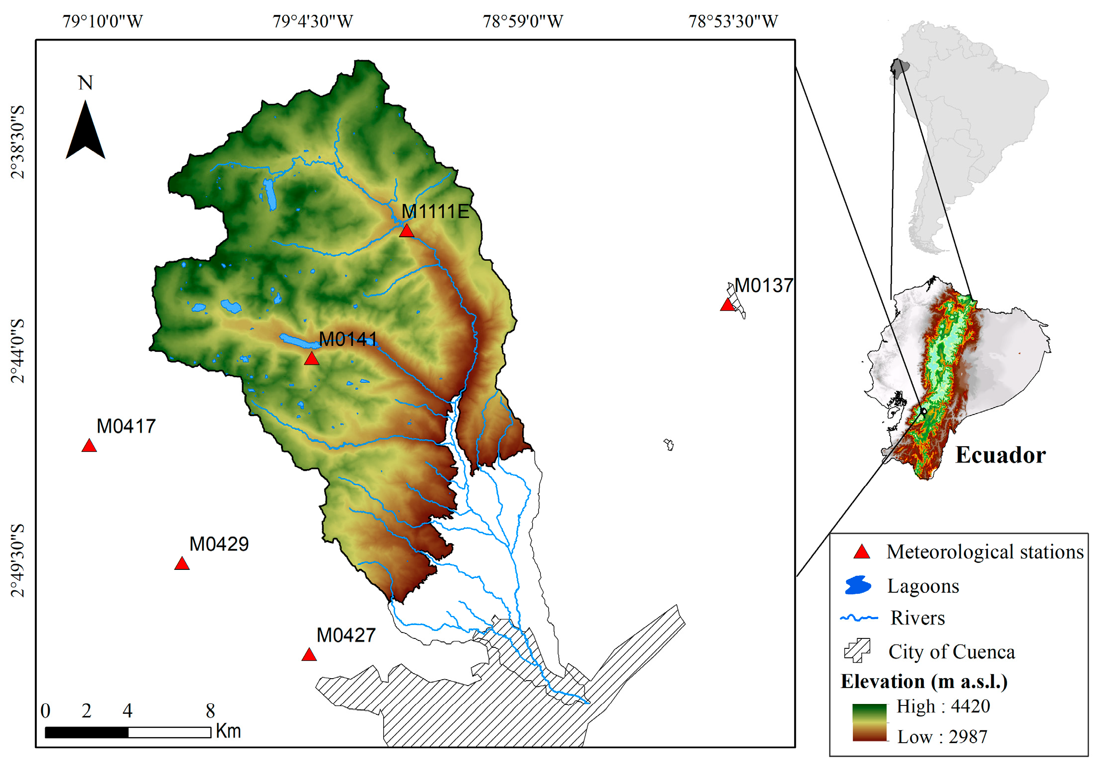
2.1. Study Area

The study area was the upper part of the Machángara river sub-basin (Figure 1), located in the Southern Ecuadorian Andes. This area covers approximately 270 km² in an inter-Andean depression, and its elevation ranges between 2987 and 4420 m.a.s.l. Temperature varies between 9 °C and 16 °C. The average annual rainfall oscillates between 877 mm in the lower and 1363 mm in the upper regions. The study area is covered chiefly with páramo (tussock grass), which plays a vital role in hydrological processes in Andean catchments [56]. The Andean montane páramo ecosystem consists of glacially-formed plains and valleys with several lakes, moist grasslands, and patches of low-lying montane forest. The Machángara river sub-basin supplies water for human consumption in Cuenca city (the third most important in Ecuador), rural settlements, agriculture irrigation, industrial use, and electricity generation [58].

2.2. Data

2.2.1. Meteorological Stations Data

Monthly data on precipitation and maximum and minimum temperature were obtained from meteorological stations of the National Institute of Meteorology and Hydrology of Ecuador (INAMHI—https://www.inamhi.gob.ec, accessed on 28 January 2021) from 1981–2015 (Figure 1).

2.2.2. Vegetation Data

The Moderate Resolution Imaging Spectroradiometer (MODIS), developed by the National Aeronautics and Space Administration (NASA), provides satellite data for improving the understanding of the Earth system [64]. The product used was MOD13Q1–NDVI from MODIS-Terra (https://modis.gsfc.nasa.gov, accessed on 8 December 2022). In this research, the monthly MODIS data configured a time series (2001–2015) of NDVI records with a spatial resolution of 250 m and 16 days of temporal resolution.

2.2.3. ENSO Indexes

The ENSO indexes of the Pacific Ocean regions were used to explain the relationships between the ENSO phenomenon and drought and vegetation. The data for ENSO is accessible online at https://psl.noaa.gov/data/climateindexes/list, accessed on 12 March 2021.

ENSO is an alteration of the ocean-atmosphere system in the tropical Pacific that has significant consequences on the climate around the planet. ENSO fluctuates between the El Niño warm and La Niña cold phases [65]. Owing to the complexity of ENSO, there are different indexes based on sea surface temperature (SST) and atmospheric pressure. The temperature-based indexes are named according to the location in the Pacific Ocean. According to National Oceanic and Atmospheric Administration (NOAA), the definition of indexes are:

Niño 1 + 2 (0–10 S, 90 W–80 W): The Niño 1 + 2 region comprises a small part of the coastal area of South America (Ecuador and part of Perú). This index shows the highest variation of the El Niño SST indexes.

Niño 3 (5 N–5 S, 150 W–90 W): Niño 3 index occurs at the central Pacific. El Niño and La Niña events are defined when Niño 3 index exceeds +/−0.5 °C for six months or more.

Niño 3.4 (5 N–5 S, 170 W–120 W): Represents the average SSTs in the equatorial Pacific between Niño 3 and Niño 4 regions. El Niño or La Niña events occur when the Niño 3.4 SSTs exceed +/−0.4 °C for six months or more.

Niño 4 (5 N–5 S, 160 E–150 W): The Niño 4 index represents SST anomalies in the central equatorial Pacific. This region shows less variation than the other El Niño regions.

ONI (5 N–5 S, 170 W–120 W): The Oceanic Niño Index considers the same region as the Niño 3.4 index. ONI classifies El Niño o La Niña events when SSTs exceed +/−0.5 °C for five consecutive months. According to the ONI index classification (https://ggweather.com/enso/oni.htm, accessed on 13 May 2022), years from 1951 to 2021 were classified as ENSO years (El Niño and La Niña) with categories: weak, moderate, strong, or very strong.

The Southern Oscillation Index (SOI) is a result of the difference in standardized atmospheric pressure between two islands: Tahiti (eastern-central part of the Tropical Pacific) and Darwin (western part of the Tropical Pacific).

2.3. Methodology

2.3.1. Meteorological Drought through Standardized Precipitation and Evapotranspiration Index (SPEI)

The SPEI considers the effect of increased temperature on droughts [66] using its influence on both precipitation and potential evapotranspiration (PET) [67]. The SPEI index is simple to calculate and multi-scalar, which makes it easy to link with various phases of drought [68,69]. Three methods are commonly used for calculating PET, depending on data availability: Penman-Monteith, which incorporates solar radiation, relative humidity, and wind speed [70,71]. The Thornthwaite method requires the latitude and mean daily temperature of the location [72,73]. Hargreaves method request latitude and daily minimum and maximum temperature [74,75]. Several studies have evidenced that the choice of PET does not affect the drought stages; however, PET computation could affect the intensity of drought [76,77,78]. Although Penman-Monteith produces good results in Andean regions [79], we apply the Hargreaves method due to the unavailability of data. The following steps for SPEI calculations were performed: (1) The Inverse Distance Weighting (IDW) method was used to generate a spatial distribution of precipitation, minimum and maximum temperature, with a spatial resolution of 250 m at the same scale as the NDVI [80,81]. (2) PET was calculated by the Hargreaves method; (3) water balance was the result of subtracting total monthly precipitation and PET; (4) the SPEI values at time scales of 1, 3 and 6 months were calculated using the R SPEI package (http://cran.r-project.org/web/packages/SPEI, accessed on 17 February 2021). Further details of the SPEI calculation can be found in Vicente-Serrano et al. (2010). Positive values denote drought absence, and negative values (≤–0.9) represent different levels of drought. The SPEI values and category ranges are shown in

Table 1. Categorization of the SPEI index.

SPEI Values	Category
>2	Extremely humid
1.99–1.50	Very humid
1.49–1.00	Moderately humid
0.99–−0.99	Normal
−1.00–−1.49	Moderate drought
−1.50–−1.99	Severe drought
<−2.00	Extreme drought

[80,81].

2.3.2. Vegetation Index (NDVI)

Due to the presence of some unreliable pixels in the original satellite images from MODIS, we have discarded the unreliable pixels (no data, snow, and cloudy) [82], according to the MOD13 User Guide [83]. The moving window method was used to eliminate information gaps, filling these with the average of the surrounding pixels using a 3 × 3 window [84]. In addition, since the MODIS images have a temporal resolution of 16 days, the values were monthly by mean of two images per month to have comparable series with SPEI data. Monthlyizing the NDVI data minimizes some effects of cloud cover, atmospheric interference, and solar zenith angle [82,85]. The NDVI takes values between −1 and 1. Water takes values near −1, and bare soil, urban areas, and rock take negative values close to zero. Positive values greater than 0.2 represent areas with good vegetation and grasslands [86,87]. We determine the final monthly value of NDVI by calculating the average value per MODIS satellite image. The steps mentioned above were followed for all MODIS images in the data series.

2.3.3. Wavelet Correlation

The association between SPEI, NDVI, and ENSO indexes was examined using wavelet cross-correlation. The Wavelet methodology is a helpful tool for studying periodic phenomena in time series, including the time and frequency resolution predicament, and it is considered a shift in signal and image processing [88,89]. Wavelet provides robust time-frequency analysis but only identifies features of a single time series [90]. Wavelet coherence (WTC) analyzes the cross-correlation between two-time series, $x$ and $y$, in the time-frequency domain [21]. The WTC [91,92] can be defined as:

$$R_n^2\left(a\right) = \frac{{\left|S\left(a^{-1}{W}_n^{xy}\left(a\right)\right)\right|}^2}{S(a^{-1}|W_n^x\left(a\right){|}^2)(a^{-1}|W_n^y\left(a\right){|}^2)}$$

(1)

According to Zhou [21], $W_n^{xy}$ represents the cross-wavelet power spectrum. $W_n^{xy}$ is the wavelet transforms for $x$ and $y$ time series. $S$ is a smoothing operator of the time series. $R_n^2\left(a\right)$ represents a number between 0 and 1. A value of 1 denotes a significant correlation between $x$ and $y$. A value of 0 indicates there is no correlation between the two time sequences. Detailed descriptions of the power spectrum, cross-wavelet transform, and the $S$ operator can be found in Torrence [92] and Grinsted [93]. WTC was calculated using the R WaveletComp package [94].

3. Results

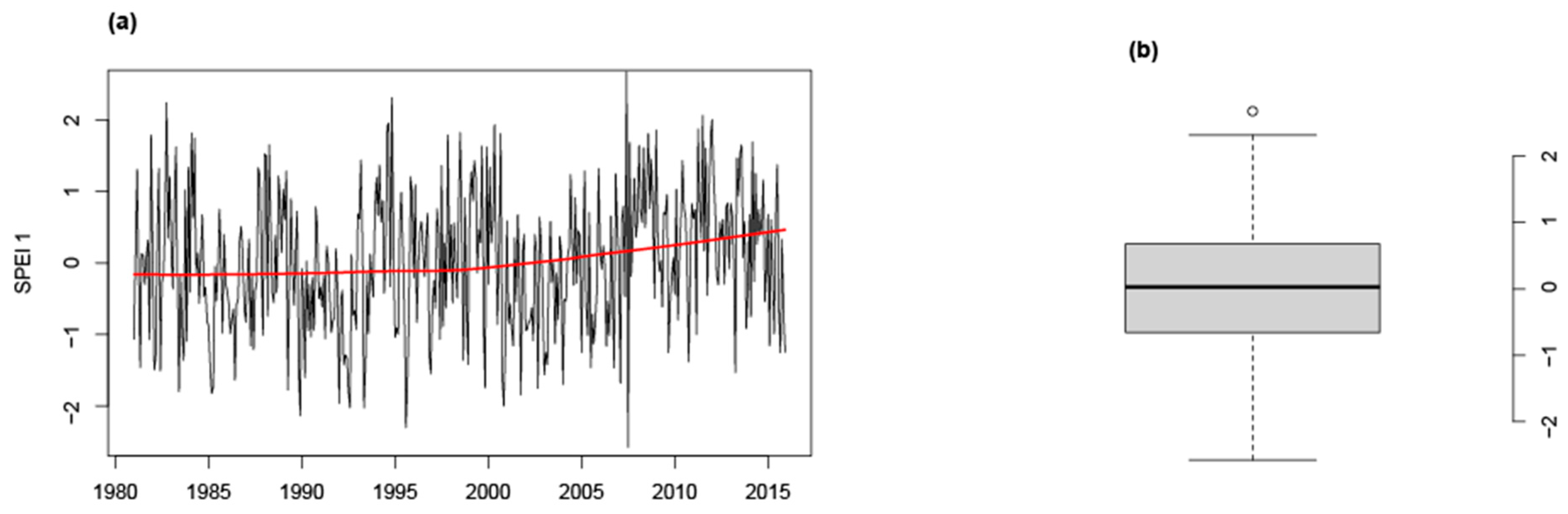
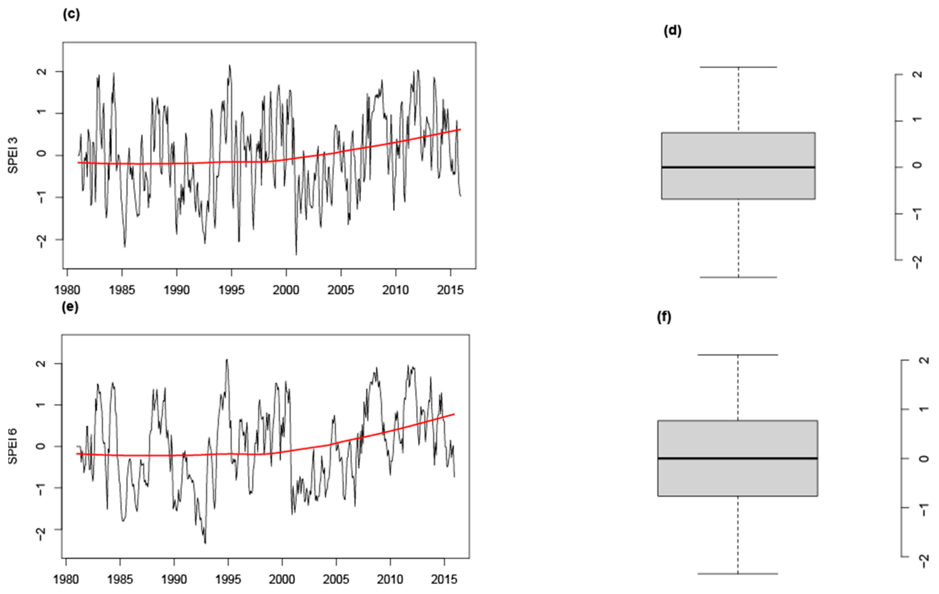
3.1. Meteorological Drought Events

Figure 2 shows the SPEI index with a scale of 1, 3 and 6 months. The index showed that the most severe droughts occurred in July/2007 (−2.57/SPEI1), December/1992 (−2.36/SPEI 3), and December/1992 (−2.35/SPEI6). Most of the dry events were one month, and the most extended duration was five months, which occurred in August–December 1992 for SPEI 6. All the time series presented a positive trend and a similar distribution (Figure 2).

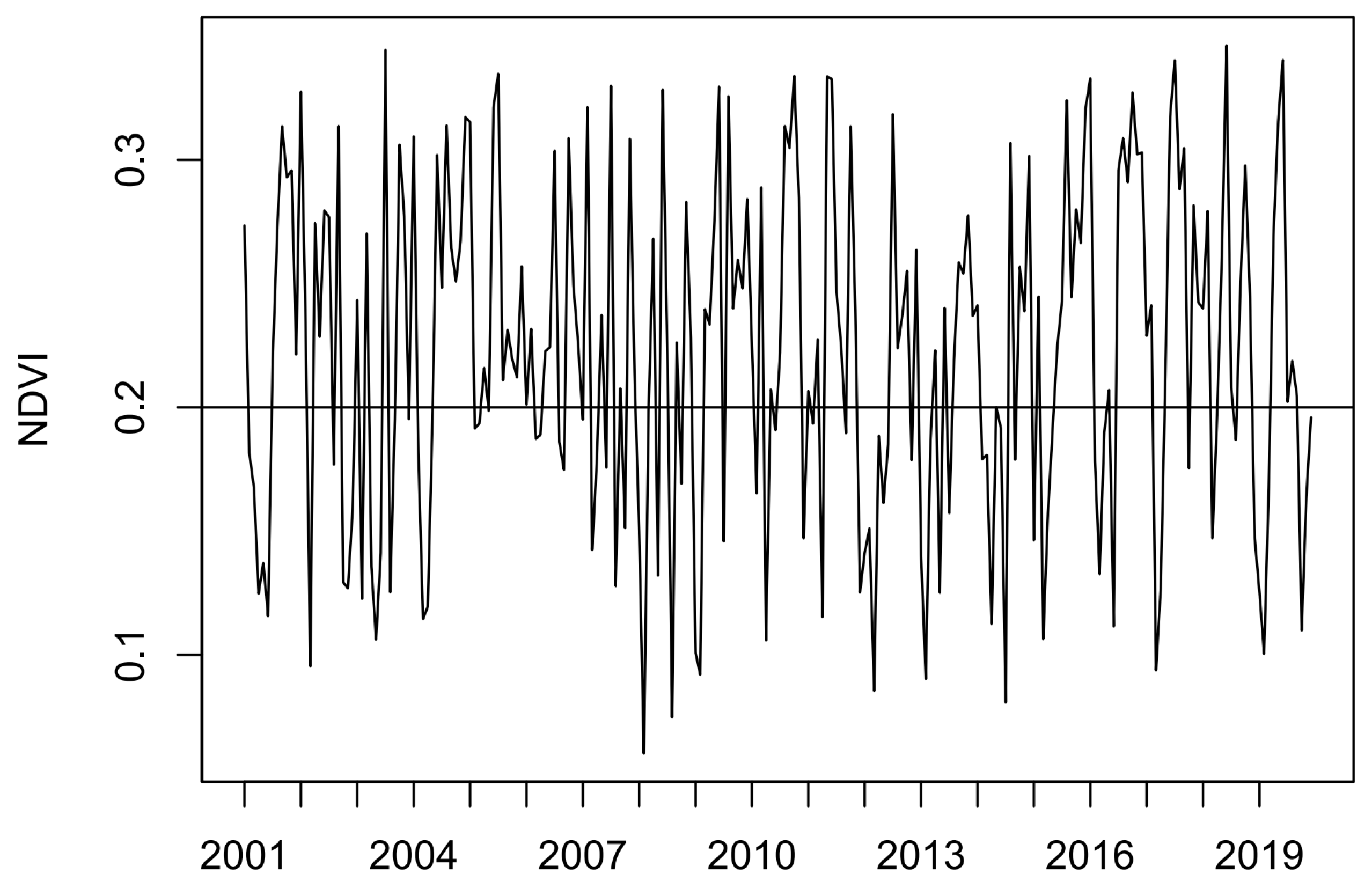
3.2. Characterization of the Vegetation

The NDVI between 2001–2019 in the upper area of the Machángara sub-basin is shown in Figure 3. The lowest NDVI (<0.2) was presented in February, March and April in 2008, 2009, 2012, 2013 and 2014. The 67% of events were categorized as good vegetation cover, prairies, and grasslands (NDVI ˃ 0.2).

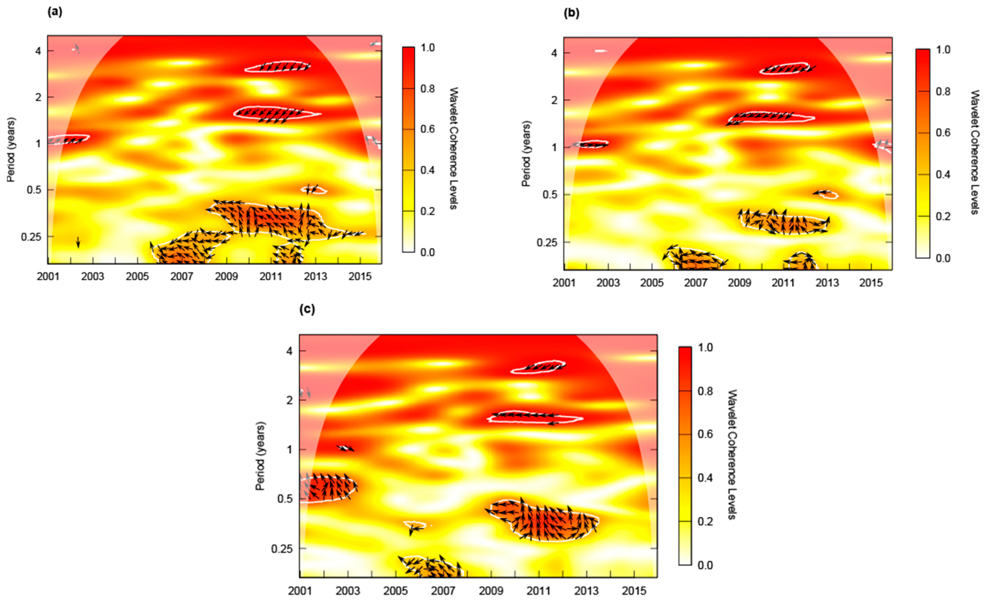
3.3. Relations between Droughts and Vegetation

Note that for all wavelet correlation figures, significant consistencies at 5% are outlined in white inside the cone of influence delimited by the shaded area within which colors are most vivid. Additionally, we reported the best-averaged correlations outlined in white (higher than 0.7). Within the boxed section are left-pointing arrows indicating a negative relationship ($x$ and $y$ time series are in antiphase) and right-pointing arrows indicating a positive relationship ($x$ and $y$ time series are in phase). An antiphase relationship with an up-pointing arrow represents $y$ is leading (ahead) the relationship, and $x$ is lagging (delay); a down-pointing arrow denotes $x$ is leading, and $y$ is lagging. A phase relationship with an up-pointing arrow indicates that $x$ is leading and $y$ is lagging; a down-pointing arrow represents that $y$ is leading and $x$ is lagging the relationship [91]. Phase difference represents the time in months a variable leads or lags in significant return periods.

Our study found negative/anti-phase correlations between SPEI and NDVI at different return periods. Figure 4a–c show good correlations (~0.8) between 2009–2013, with a return period of around 1.5 years. SPEI1 and SPEI3 were the leading variables. Only SPEI6 was lagging by nine months. On the other hand, between 2010–2012 and 2009–2013, with a return period of around three years and 0.35 years, respectively, correlations are not significant.

Between 2009 and 2013, for SPEI1, five drought events with an average index of −1.27 were reported. The driest month was October 2010, with −1.43. For SPEI3, two drought events were evidenced with an average index of −1.26. The driest month was November 2011, with −1.27. For SPEI6, the values remained within the normal range. NDVI reported the lowest indexes in 2008, 2009, 2012, 2013 and 2014.

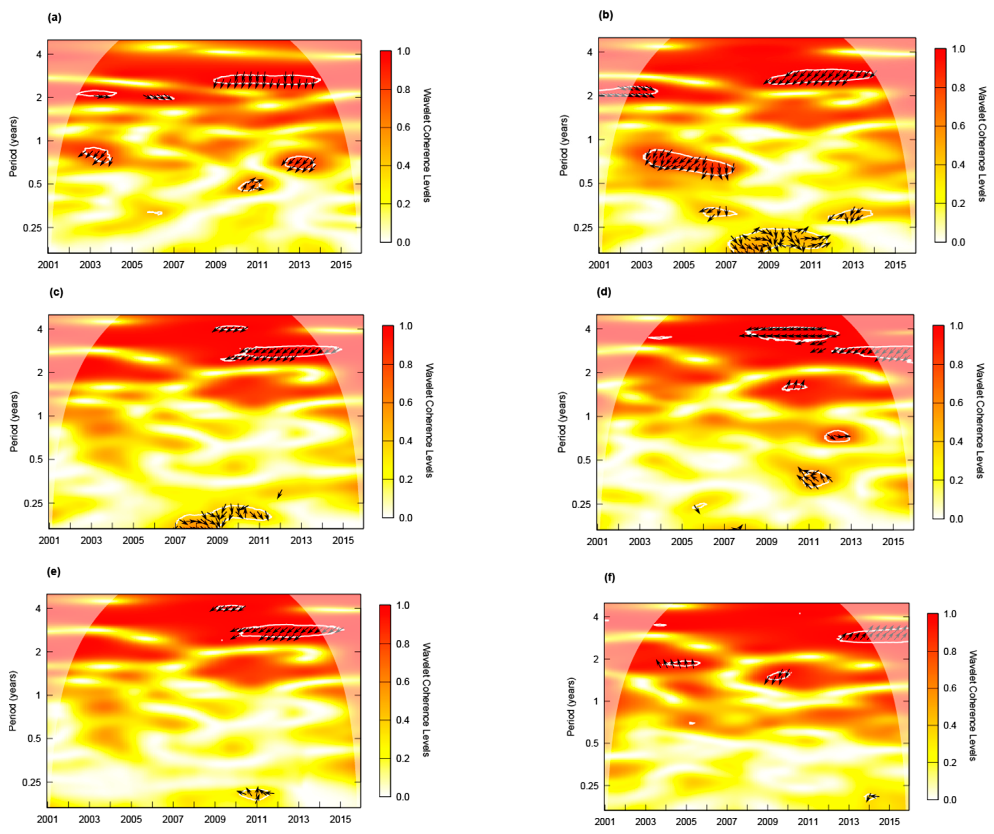
3.4. Relations between ENSO and Drought

The WTC between Niño 1 + 2, Niño 3, Niño 3.4, Niño 4, ONI and SOI index, and SPEI1 is shown in Figure 5. In general, ENSO–SPEI1, SPEI3 and SPEI6 relationships showed similar results in time and frequency.

Niño 1 + 2 and SPEI1 maintained a negative correlation of around 0.8 during 2009–2013. The return period was approximately three years (Figure 5a).

Niño 3 and SPEI1 were negatively correlated (Figure 5b). The highest correlation (~0.9) occurred between 2009–2014, around three years of the return period. SPEI presented a delay of 14 months.

The Niño 3.4 and SPEI1 presented a negative relationship (Figure 5c). During 2010–2014 and around three years of the return period, SPEI1 lagged by 14 months. A similar situation is displayed in Figure 5d; at Niño 4–SPEI1 relationship SPEI1 is delayed around 20 months during 2009–2012.

The relationship between ONI and SPEI1 is shown in Figure 5e. In the three years of the return period, a negative correlation (higher than 0.9 on average) was found between 2010 and 2014; ONI led the relationship by 15 months.

A positive correlation (~0.9 on average) between SOI and SPEI1 was found in the three years return period (Figure 5f). Nevertheless, only a short section of this correlation (2013–2014) was inside the cone of influence. SOI was leading the relationship for 15 months.

The correlations above showed (ENSO–SPEI1) presented typical time intervals from 2009 to 2012 and 2009 to 2014 with significant consistencies at 5%.

During 2009–2014, two El Niño years occurred, one year was categorized as moderate, and one was weak. On the other hand, two La Niña years were presented, one year was classified as strong, and one year was moderate. Also, two neutral years occurred.

Between 2009–2012, one moderate El Niño year occurred. In contrast, two La Niña years presented, one year was strong, and one year was moderate. One neutral year was also presented.

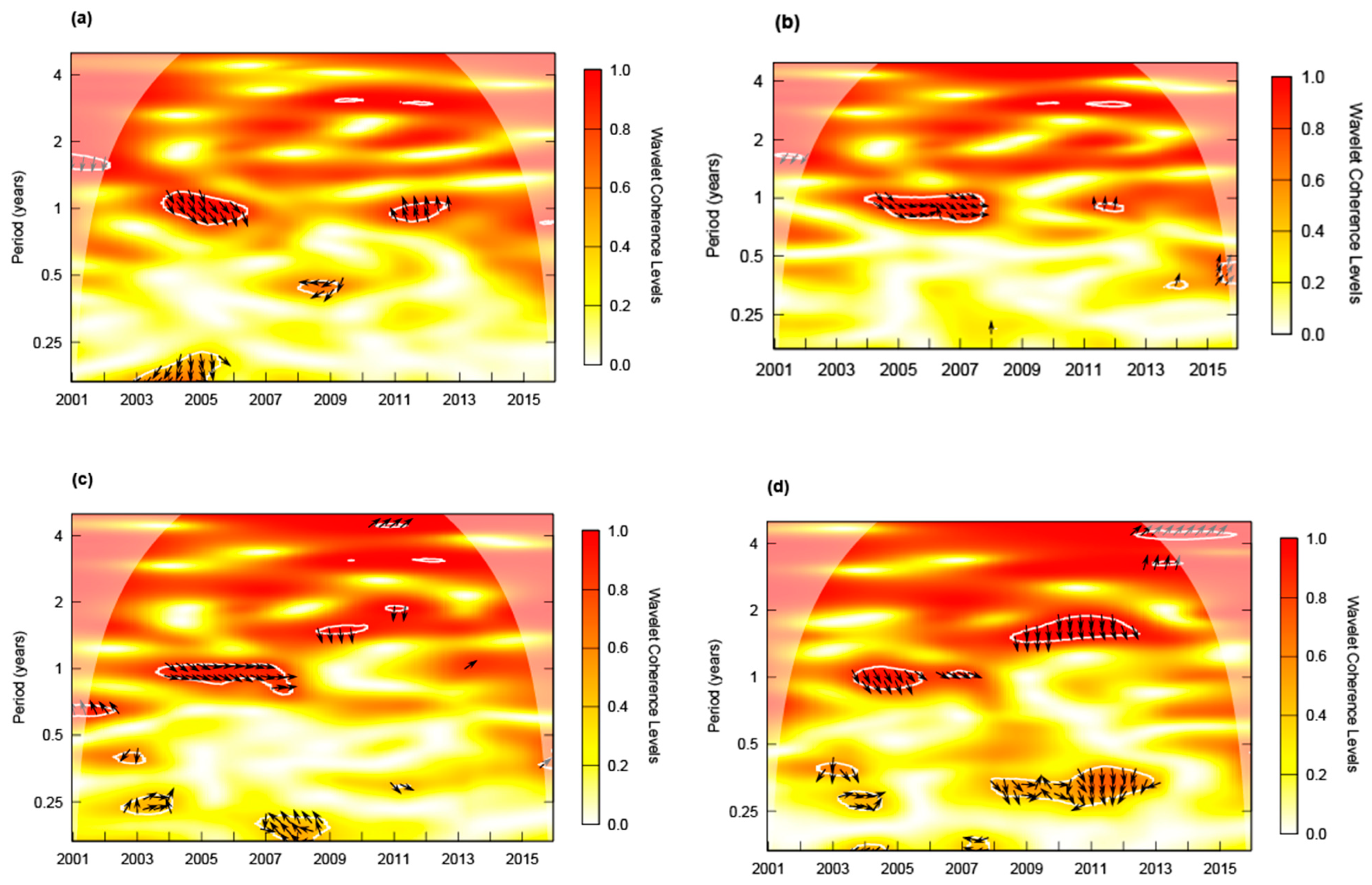
3.5. Relations between ENSO and Vegetation

The WTC between Niño 1 + 2, Niño 3, Niño 3.4, Niño 4, ONI and SOI index, and NDVI are represented in Figure 6, from which we can notice the relationships between ENSO and vegetation. All correlations were positive, and NDVI was the leading variable.

The relationship between Niño 1 + 2 and NDVI is represented in Figure 6a. The most relevant correlation, around 0.7, occurred in the return period of one year. Between 2004 and 2006, Niño 1 + 2 was delayed by approximately 2.4 months.

For both relationships, Niño 3–NDVI (Figure 6b) and Niño 3.4–NDVI (Figure 6c) the highest correlation (~0.7) occurred between 2004–2008 and around one year of the return period. ENSO presented a delay of 1 month.

The Niño 4–NDVI relationship is shown in Figure 6d. Two time intervals were observed: from 2009 to 2012, with a return period of ~1.5 years and a correlation of ~0.7. From 2004 to 2006, with a return period of one year and a correlation around 0.6. Niño 4 presented a delay of approximately 3 and 2.4 months, respectively. Relationships between ONI-NDVI and SOI-NDVI were diffuse and not significant.

Between 2004–2006, two weak El Niño years occurred, and one La Niña year was presented. Between 2004–2008, also two weak El Niño years occurred. In contrast, two weak La Niña years were presented, and one year was strong.

4. Discussion

In the Machángara sub-basin, a high-altitude area with a humid climate, the results show that SPEI1 and SPEI3 lead the negative relationships with NDVI and only SPEI6 start to change by lagging. The results above agree with those reported by other authors [26,27,95], who found that in high and semi-humid zones, the aggregated impacts of meteorological drought on vegetation occurred primarily in medium terms (from five to eight months). Lagged vegetation reaction to meteorological drought (SPEI1 and SPEI3) refers to factors such as vegetation type or the surrounding environment (temperature, soil moisture) [96]. Moreover, in humid zones, the NDVI is impacted by meteorological drought in longer months (SPEI6) due to accumulated episodes of drought (one to five months). One to three months-drought does not affect NDVI immediately [97]. Zhan et al. [26] and Zhao et al. [27] found that accumulated drought (from five to eight months) is typical of semi-humid regions and grasslands’ response to drought between four and six months. Therefore, Machángara vegetation cover (mostly páramo and grassland) has soil moisture retention effects so that it would withstand the impact of meteorological drought well; this could be why SPEI1 and SPEI3 are advanced in the correlation, while SPEI6 is lagging.

The correlations found with ENSO and SPEI coincide in being negative with other studies [38,41,98]. Our results corroborate the findings of Vicente-Serrano [38] that Niño 1 + 2 index does not cause SPEI anomalies in the Andes. In addition, La Niña provokes humid states in the Ecuadorian Andes and enhances the convective process and moisture transport from the Amazonas basin to the Andes. Therefore, higher cloud cover may contribute decrease evapotranspiration during La Niña years. Another coincidence was with the study of Ávila and Ballari [39], who found that the climatic indexes lead to the relationship between precipitation and ENSO. Nieves et al. [63] also found a negative correlation between ENSO and meteorological drought in an Andean catchment simultaneously (2009–2012) and a similar return period. Nonetheless, drought is more delayed when PET gets involved. Contrary to our results, studies affirm that drought was positively related to extreme episodes during El Niño events in the Northen tropical Andes [99,100,101]. On the other hand, Mo and Schemm [40] reported a seasonally dependent behavior between ENSO and drought, where cold ENSO induces drought events in winter but probably brings precipitations in summer.

In general, our results showed that the impact of ENSO on vegetation had a lag effect, this agrees with Yan et al. [49], and Poveda et al. [47], who established that vegetation was always leading the relationships. Contrary to our results Erasmi et al. [22]. Our findings showed that the highest correlation between ENSO–NDVI was around 0.7. Only ONI and SOI showed no significant relationships in contrast with Casa et al. [28]. However, ENSO does not always influence vegetation. Erasmi et al. [22] found that vegetation reacted to ENSO for moderate-strong El Niño events, and weak El Niño events showed no clear patterns. As aforementioned, the vegetation in the tropics probably does not respond significantly to ENSO events due to consecutive short-term changes between El Niño and La Niña periods. Our results show that tropical vegetation maintains a positive correlation with ENSO events. Due to El Niño (warm phase) provokes droughts in Andean Ecuadorian regions, and La Niña (cold phase) enhances precipitations through convective processes [38]. Therefore, vegetation reacts to El Niño and La Niña by improving or deteriorating its greenness. However, after an El Niño event, the presence of a La Niña event enhances vegetation in other regions [49].

5. Conclusions

This research analyzed the relationships between meteorological drought, vegetation, and the influence of ENSO. Wavelet coherence was used to determine the value of the correlation, the lags/leads of the variables, the return periods, and the time lapses when the correlation occurred.

SPEI–NDVI relationship described a negative correlation with SPEI1 and SPEI3 leading; only SPEI6–NDVI presented a significant correlation, with SPEI6 delayed around nine months. Humid conditions of the Machángara sub-basin influence the vegetation response to meteorological drought. This tropical Andean sub-basin evidence moisture retention on soil and vegetation, so the meteorological drought impact on vegetation is not immediate.

ENSO–SPEI relationships were always negative. In general, ENSO-SPEI1, ENSO-SPEI3, and ENSO-SPEI6 showed similar results in time and frequency. However, only SPEI1 evidenced a significant delay of around 14 months. Moreover, the highest correlation (~0.9) was obtained between 2009 and 2014 in the three-year return period.

ENSO–NDVI relationships presented a positive correlation; this condition is due to the stable conditions of tropical regions. The years between 2004 and 2008 were the most common years, and significant correlations were registered in one year of the return period. ENSO was constantly delayed by around 1.2 months. El Niño presented two weak years in this time-lapse, and La Niña presented one strong and two weak years. ENSO–NDVI relationship was more evident when a strong event occurred.

This research has enhanced our comprehension of the relationships and impacts of drought–vegetation–ENSO on the Machángara subbasin. However, there are still unknown issues, for instance, assessing drought considering other vegetation types in the Andean region (different locations, climates, and humid conditions). Another excellent effort would involve drought intensity and frequency for determining the response characteristics of vegetation. In addition, we used 15 years, up to 2015. Hence, extending the time to capture more robust relations between variables is necessary to clarify some knowledge gaps.

References

1. UNESCO; UN-WATER. United Nations World Water Development Report 2020:Water and Climate Change; UNESCO: Paris, France, 2020. [Google Scholar]
2. Van Loon, A.F.; Gleeson, T.; Clark, J.; Van Dijk, A.I.J.M.; Stahl, K.; Hannaford, J.; Di Baldassarre, G.; Teuling, A.J.; Tallaksen, L.M.; Uijlenhoet, R.; et al. Drought in the Anthropocene. Nat. Geosci. 2016, 9, 89–91. [Google Scholar] [CrossRef] [Green Version]
3. Mishra, A.K.; Singh, V.P. A Review of Drought Concepts. J. Hydrol. 2010, 391, 202–216. [Google Scholar] [CrossRef]
4. Van Loon, A.F.; Stahl, K.; Di Baldassarre, G.; Clark, J.; Rangecroft, S.; Wanders, N.; Gleeson, T.; Van Dijk, A.I.J.M.; Tallaksen, L.M.; Hannaford, J.; et al. Drought in a Human-Modified World: Reframing Drought Definitions, Understanding, and Analysis Approaches. Hydrol. Earth Syst. Sci. 2016, 20, 3631–3650. [Google Scholar] [CrossRef] [Green Version]
5. Paulo, A.A.; Pereira, L.S. Drought Concepts and Characterization: Comparing Drought Indices Applied at Local and Regional Scales. Water Int. 2006, 31, 37–49. [Google Scholar] [CrossRef]
6. Hao, Z.; Singh, V.P. Drought Characterization from a Multivariate Perspective: A Review. J. Hydrol. 2015, 527, 668–678. [Google Scholar] [CrossRef]
7. Wilhite, D.A.; Glantz, M.H. Understanding: The Drought Phenomenon: The Role of Definitions *. Water Int. 1985, 10, 111–120. [Google Scholar] [CrossRef] [Green Version]
8. Van Loon, A.F. Hydrological Drought Explained. Wiley Interdiscip. Rev. Water 2015, 2, 359–392. [Google Scholar] [CrossRef]
9. Wu, J.; Chen, X.; Yao, H.; Gao, L.; Chen, Y.; Liu, M. Non-Linear Relationship of Hydrological Drought Responding to Meteorological Drought and Impact of a Large Reservoir. J. Hydrol. 2017, 551, 495–507. [Google Scholar] [CrossRef]
10. Pedro-Monzonís, M.; Solera, A.; Ferrer, J.; Estrela, T.; Paredes-Arquiola, J. A Review of Water Scarcity and Drought Indexes in Water Resources Planning and Management. J. Hydrol. 2015, 527, 482–493. [Google Scholar] [CrossRef] [Green Version]
11. Yao, N.; Li, Y.; Lei, T.; Peng, L. Drought Evolution, Severity and Trends in Mainland China over 1961–2013. Sci. Total Environ. 2018, 616–617, 73–89. [Google Scholar] [CrossRef]
12. Ivits, E.; Horion, S.; Fensholt, R.; Cherlet, M. Drought Footprint on European Ecosystems between 1999 and 2010 Assessed by Remotely Sensed Vegetation Phenology and Productivity. Glob. Chang. Biol. 2014, 20, 581–593. [Google Scholar] [CrossRef] [PubMed]
13. Deng, S.; Chen, T.; Yang, N.; Qu, L.; Li, M.; Chen, D. Spatial and Temporal Distribution of Rainfall and Drought Characteristics across the Pearl River Basin. Sci. Total Environ. 2018, 619–620, 28–41. [Google Scholar] [CrossRef] [PubMed]
14. Jiang, Y.; Wang, R.; Peng, Q.; Wu, X.; Ning, H.; Li, C. The Relationship between Drought Activity and Vegetation Cover in Northwest China from 1982 to 2013. Nat. Hazards 2018, 92, 145–163. [Google Scholar] [CrossRef]
15. Tian, L.; Yuan, S.; Quiring, S.M. Evaluation of Six Indices for Monitoring Agricultural Drought in the South-Central United States. Agric. For. Meteorol. 2018, 249, 107–119. [Google Scholar] [CrossRef]
16. Araneda-Cabrera, R.J.; Bermudez, M.; Puertas, J. Revealing the Spatio-Temporal Characteristics of Drought in Mozambique and Their Relationship with Large-Scale Climate Variability. J. Hydrol. Reg. Stud. 2021, 38, 100938. [Google Scholar] [CrossRef]
17. Kalisa, W.; Igbawua, T.; Henchiri, M.; Ali, S.; Zhang, S.; Bai, Y.; Zhang, J. Assessment of Climate Impact on Vegetation Dynamics over East Africa from 1982 to 2015. Sci. Rep. 2019, 9, 16865. [Google Scholar] [CrossRef] [Green Version]
18. Zhao, J.; Huang, S.; Huang, Q.; Wang, H.; Leng, G.; Fang, W. Time-Lagged Response of Vegetation Dynamics to Climatic and Teleconnection Factors. Catena 2020, 189, 104474. [Google Scholar] [CrossRef]
19. Piao, S.; Wang, X.; Park, T.; Chen, C.; Lian, X.; He, Y.; Bjerke, J.W.; Chen, A.; Ciais, P.; Nemani, R.R.; et al. Characteristics, Drivers and Feedbacks of Global Greening. Nat. Rev. Earth Environ. 2020, 1, 14–27. [Google Scholar] [CrossRef] [Green Version]
20. Jiang, B.; Liang, S.; Yuan, W. Observational Evidence for Impacts of Vegetation Change on Local Surface Climate over Northern China Using the Granger Causality Test. J. Geophys. Res. Biogeosci. 2015, 120, 1–12. [Google Scholar] [CrossRef]
21. Zhou, Z.; Liu, S.; Ding, Y.; Fu, Q.; Wang, Y.; Cai, H.; Shi, H. Assessing the Responses of Vegetation to Meteorological Drought and Its Influencing Factors with Partial Wavelet Coherence Analysis. J. Environ. Manag. 2022, 311, 114879. [Google Scholar] [CrossRef]
22. Erasmi, S.; Propastin, P.; Kappas, M.; Panferov, O. Spatial Patterns of NDVI Variation over Indonesia and Their Relationship to ENSO Warm Events during the Period 1982-2006. J. Clim. 2009, 22, 6612–6623. [Google Scholar] [CrossRef]
23. Nemani, R.R.; Keeling, C.D.; Hashimoto, H.; Jolly, W.M.; Piper, S.C.; Tucker, C.J.; Myneni, R.B.; Running, S.W. Climate-Driven Increases in Global Terrestrial Net Primary Production from 1982 to 1999. Science (80-.) 2003, 300, 1560–1563. [Google Scholar] [CrossRef] [PubMed] [Green Version]
24. Wang, S.; Li, R.; Wu, Y.; Zhao, S. Effects of Multi-Temporal Scale Drought on Vegetation Dynamics in Inner Mongolia from 1982 to 2015, China. Ecol. Indic. 2022, 136, 108666. [Google Scholar] [CrossRef]
25. Bento, V.A.; Trigo, I.F.; Gouveia, C.M.; DaCamara, C.C. Contribution of Land Surface Temperature (TCI) to Vegetation Health Index: A Comparative Study Using Clear Sky and All-Weather Climate Data Records. Remote Sens. 2018, 10, 1324. [Google Scholar] [CrossRef] [Green Version]
26. Zhan, C.; Liang, C.; Zhao, L.; Jiang, S.; Niu, K.; Zhang, Y. Drought-Related Cumulative and Time-Lag Effects on Vegetation Dynamics across the Yellow River Basin, China. Ecol. Indic. 2022, 143, 109409. [Google Scholar] [CrossRef]
27. Zhao, A.; Yu, Q.; Feng, L.; Zhang, A.; Pei, T. Evaluating the Cumulative and Time-Lag Effects of Drought on Grassland Vegetation: A Case Study in the Chinese Loess Plateau. J. Environ. Manag. 2020, 261, 110214. [Google Scholar] [CrossRef]
28. de la Casa, A.; Ovando, G.; Díaz, G. Linking Data of ENSO, NDVI-MODIS and Crops Yield as a Base of an Early Warning System for Agriculture in Córdoba, Argentina. Remote Sens. Appl. Soc. Environ. 2021, 22, 100480. [Google Scholar] [CrossRef]
29. Oliveira-Júnior, J.F.; Gois, G.; Terassi, P.M.; Silva Junior, C.A.; Blanco, C.J.C.; Sobral, B.S.; Gasparini, K.A.C. Drought Severity Based on the SPI Index and Its Relation to the ENSO and PDO Climatic Variability Modes in the Regions North and Northwest of the State of Rio de Janeiro—Brazil. Atmos. Res. 2018, 212, 91–105. [Google Scholar] [CrossRef]
30. Araneda-Cabrera, R.J.; Bermudez, M.; Puertas, J. Índices De Precipitación Y Vegetación Estandarizados Bivariables Para Evaluar Y Monitorear Sequías Agrícolas. Rev. Hidrolatinoamericana 2021, 5, 27–30. [Google Scholar]
31. Liu, Z.; Li, C.; Zhou, P.; Chen, X. A Probabilistic Assessment of the Likelihood of Vegetation Drought under Varying Climate Conditions across China. Sci. Rep. 2016, 6, 35105. [Google Scholar] [CrossRef] [Green Version]
32. Brown, M.E.; de Beurs, K.; Vrieling, A. The Response of African Land Surface Phenology to Large Scale Climate Oscillations. Remote Sens. Environ. 2010, 114, 2286–2296. [Google Scholar] [CrossRef]
33. Wang, C.; Deser, C.; Yu, J.Y.; DiNezio, P.; Clement, A. El Niño and Southern Oscillation (ENSO): A Review. In Coral Reefs of the Eastern Tropical Pacific; Springer: Dordrecht, The Netherlands, 2017; Volume 8, pp. 85–106. ISBN 978-94-017-7498-7. [Google Scholar]
34. Yun, K.S.; Timmermann, A. Decadal Monsoon-ENSO Relationships Reexamined. Geophys. Res. Lett. 2018, 45, 2014–2021. [Google Scholar] [CrossRef] [Green Version]
35. Yulaeva, E.; Wallace, J.M. The Signature of ENSO in Global Temperature and Precipitation Fields Derived from the Microwave Sounding Unit. J. Clim. 1994, 7, 1719–1736. [Google Scholar] [CrossRef]
36. Gupta, V.; Jain, M.K. Unravelling the Teleconnections between ENSO and Dry/Wet Conditions over India Using Nonlinear Granger Causality. Atmos. Res. 2021, 247, 105168. [Google Scholar] [CrossRef]
37. Imfeld, N.; Barreto Schuler, C.; Correa Marrou, K.M.; Jacques-Coper, M.; Sedlmeier, K.; Gubler, S.; Huerta, A.; Brönnimann, S. Summertime Precipitation Deficits in the Southern Peruvian Highlands since 1964. Int. J. Climatol. 2019, 39, 4497–4513. [Google Scholar] [CrossRef]
38. Vicente-Serrano, S.M.; Aguilar, E.; Martínez, R.; Martín-Hernández, N.; Azorin-Molina, C.; Sanchez-Lorenzo, A.; El Kenawy, A.; Tomás-Burguera, M.; Moran-Tejeda, E.; López-Moreno, J.I.; et al. The Complex Influence of ENSO on Droughts in Ecuador. Clim. Dyn. 2017, 48, 405–427. [Google Scholar] [CrossRef] [Green Version]
39. Ávila, R.; Ballari, D. A Bayesian Network Approach to Identity Climate Teleconnections within Homogeneous Precipitation Regions in Ecuador. In Proceedings of the Conference on Information Technologies and Communication of Ecuador, Quito, Ecuador, 3–5 December 2019; Springer: Berlin/Heidelberg, Germany, 2019; pp. 21–35. [Google Scholar]
40. Mo, K.C.; Schemm, J.E. Relationships between ENSO and Drought over the Southeastern United States. Geophys. Res. Lett. 2008, 35, 1–5. [Google Scholar] [CrossRef]
41. Shahid, S. Spatial and Temporal Characteristics of Droughts in the Western Part of Bangladesh. Hydrol. Process. 2008, 22, 2235–2247. [Google Scholar] [CrossRef]
42. Zolotokrylin, A.N.; Titkova, T.B.; Brito-Castillo, L. Wet and Dry Patterns Associated with ENSO Events in the Sonoran Desert from, 2000–2015. J. Arid Environ. 2016, 134, 21–32. [Google Scholar] [CrossRef]
43. Hagemans, K.; Urrego, D.H.; Gosling, W.D.; Rodbell, D.T.; Wagner-Cremer, F.; Donders, T.H. Intensification of ENSO Frequency Drives Forest Disturbance in the Andes during the Holocene. Quat. Sci. Rev. 2022, 294, 107762. [Google Scholar] [CrossRef]
44. Hao, Y.; Hao, Z.; Feng, S.; Zhang, X.; Hao, F. Response of Vegetation to El Niño-Southern Oscillation (ENSO) via Compound Dry and Hot Events in Southern Africa. Glob. Planet. Change 2020, 195, 103358. [Google Scholar] [CrossRef]
45. Propastin, P.; Fotso, L.; Kappas, M. Assessment of Vegetation Vulnerability to ENSO Warm Events over Africa. Int. J. Appl. Earth Obs. Geoinf. 2010, 12, 83–89. [Google Scholar] [CrossRef]
46. Park, S.; Kang, D.; Yoo, C.; Im, J.; Lee, M.I. Recent ENSO Influence on East African Drought during Rainy Seasons through the Synergistic Use of Satellite and Reanalysis Data. ISPRS J. Photogramm. Remote Sens. 2020, 162, 17–26. [Google Scholar] [CrossRef]
47. Poveda, G.; Salazar, L.F. Annual and Interannual (ENSO) Variability of Spatial Scaling Properties of a Vegetation Index (NDVI) in Amazonia. Remote Sens. Environ. 2004, 93, 391–401. [Google Scholar] [CrossRef]
48. Glennie, E.; Anyamba, A. Midwest Agriculture and ENSO_Glennie2018. Pdf. Int. J. Appl. Earth Obs. Geoinf. 2018, 68, 180–188. [Google Scholar]
49. Yan, Y.; Mao, K.; Shen, X.; Cao, M.; Xu, T.; Guo, Z.; Bao, Q. Evaluation of the Influence of ENSO on Tropical Vegetation in Long Time Series Using a New Indicator. Ecol. Indic. 2021, 129, 107872. [Google Scholar] [CrossRef]
50. Myers, N.; Mittermeier, R.A.; Mittermeier, C.G.; da Fonseca, G.A.B.; Kent, J. Biodiversity Hotspots for Conservation Priorities. Nature 2000, 403, 895. [Google Scholar] [CrossRef]
51. Llambí, L.D.; Soto-W, A.; Célleri, R.; De Biévre, B.; Ochoa, B.; Borja, P. Ecología, Hidrología y Suelos de Páramos: Proyecto Páramo Andino; CONDENSAN: Quito, Ecuador, 2012. [Google Scholar]
52. Buytaert, W.; Celleri, R.; Willems, P.; De Bièvre, B.; Wyseure, G. Spatial and Temporal Rainfall Variability in Mountainous Areas: A Case Study from the South Ecuadorian Andes. J. Hydrol. 2006, 329, 413–421. [Google Scholar] [CrossRef]
53. Célleri, R.; Feyen, J. The Hydrology of Tropical Andean Ecosystems: Importance, Knowledge Status, and Perspectives. Mt. Res. Dev. 2009, 29, 350–355. [Google Scholar] [CrossRef]
54. Cincotta, R.P.; Wisnewski, J.; Engelman, R. Human Population in the Biodiversity Hotspots. Nature 2000, 404, 990–992. [Google Scholar] [CrossRef]
55. Flores-López, F.; Galaitsi, S.E.; Escobar, M.; Purkey, D. Modeling of Andean Páramo Ecosystems’ Hydrological Response to Environmental Change. Water 2016, 8, 94. [Google Scholar] [CrossRef]
56. Ochoa-Tocachi, B.F.; Buytaert, W.; De Bievre, B.; Célleri, R.; Crespo, P.; Villacís, M.; Llerena, C.A.; Acosta, L.; Villazón, M.; Guallpa, M.; et al. Impacts of Land Use on the Hydrological Response of Tropical Andean Catchments. Hydrol. Process. 2016, 30, 4074–4089. [Google Scholar] [CrossRef]
57. Avilés, A.; Célleri, R.; Paredes, J.; Solera, A. Evaluation of Markov Chain Based Drought Forecasts in an Andean Regulated River Basin Using the Skill Scores RPS and GMSS. Water Resour. Manag. 2015, 29, 1949–1963. [Google Scholar] [CrossRef] [Green Version]
58. Avilés, A.; Célleri, R.; Solera, A.; Paredes, J. Probabilistic Forecasting of Drought Events Using Markov Chain-and Bayesian Network-Based Models: A Case Study of an Andean Regulated River Basin. Water 2016, 8, 37. [Google Scholar] [CrossRef]
59. Zhiña, D.; Montenegro, M.; Montalván, L.; Mendoza, D.; Contreras, J.; Campozano, L.; Avilés, A. Climate Change Influences of Temporal and Spatial Drought Variation in the Andean High Mountain Basin. Atmosphere 2019, 10, 558. [Google Scholar] [CrossRef] [Green Version]
60. Valverde-Arias, O.; Garrido, A.; Valencia, J.L.; Tarquis, A.M. Using Geographical Information System to Generate a Drought Risk Map for Rice Cultivation: Case Study in Babahoyo Canton (Ecuador). Biosyst. Eng. 2018, 168, 26–41. [Google Scholar] [CrossRef]
61. Zambrano Mera, Y.E.; Rivadeneira Vera, J.F.; Pérez-Martín, M.Á. Linking El Niño Southern Oscillation for Early Drought Detection in Tropical Climates: The Ecuadorian Coast. Sci. Total Environ. 2018, 643, 193–207. [Google Scholar] [CrossRef]
62. Campozano, L.; Ballari, D.; Montenegro, M.; Avilés, A. Future Meteorological Droughts in Ecuador: Decreasing Trends and Associated Spatio-Temporal Features Derived From CMIP5 Models. Front. Earth Sci. 2020, 8, 17. [Google Scholar] [CrossRef]
63. Nieves, A.; Contreras, J.; Pacheco, J.; Urgilés, J.; García, F.; Avilés, A. Assessment of Drought Time-Frequency Relationships with Local Atmospheric-Land Conditions and Large-Scale Climatic Factors in a Tropical Andean Basin. Remote Sens. Appl. Soc. Environ. 2022, 26, 100760. [Google Scholar] [CrossRef]
64. Dorjsuren, M.; Liou, Y.A.; Cheng, C.H. Time Series MODIS and in Situ Data Analysis for Mongolia Drought. Remote Sens. 2016, 8, 509. [Google Scholar] [CrossRef] [Green Version]
65. Salinger, J.; Sivakumar, M.V.K.; Motha, R.P. Increasing Climate Variability and Change; Springer: Dordrecht, The Netherlands, 2005; ISBN 1402033540. [Google Scholar]
66. Vicente-Serrano, S.M.; Beguería, S.; López-Moreno, J.I. A Multiscalar Drought Index Sensitive to Global Warming: The Standardized Precipitation Evapotranspiration Index. J. Clim. 2010, 23, 1696–1718. [Google Scholar] [CrossRef] [Green Version]
67. Beguería, S.; Vicente-Serrano, S.M.; Reig, F.; Latorre, B. Standardized Precipitation Evapotranspiration Index (SPEI) Revisited: Parameter Fitting, Evapotranspiration Models, Tools, Datasets and Drought Monitoring. Int. J. Climatol. 2014, 34, 3001–3023. [Google Scholar] [CrossRef]
68. Gupta, V.; Jain, M.K. Investigation of Multi-Model Spatiotemporal Mesoscale Drought Projections over India under Climate Change Scenario. J. Hydrol. 2018, 567, 489–509. [Google Scholar] [CrossRef]
69. Wang, Y.; Liu, G.; Guo, E. Spatial Distribution and Temporal Variation of Drought in Inner Mongolia during 1901–2014 Using Standardized Precipitation Evapotranspiration Index. Sci. Total Environ. 2019, 654, 850–862. [Google Scholar] [CrossRef]
70. Feng, S.; Trnka, M.; Hayes, M.; Zhang, Y. Why Do Different Drought Indices Show Distinct Future Drought Risk Outcomes in the U. S. Great Plains? J. Clim. 2017, 30, 265–278. [Google Scholar] [CrossRef]
71. Zhang, Y.; Yu, Z.; Niu, H. Standardized Precipitation Evapotranspiration Index Is Highly Correlated with Total Water Storage over China under Future Climate Scenarios. Atmos. Environ. 2018, 194, 123–133. [Google Scholar] [CrossRef]
72. Bae, S.; Lee, S.H.; Yoo, S.H.; Kim, T. Analysis of Drought Intensity and Trends Using the Modified SPEI in South Korea from 1981 to 2010. Water 2018, 10, 327. [Google Scholar] [CrossRef] [Green Version]
73. Bonsal, B.R.; Cuell, C.; Wheaton, E.; Sauchyn, D.J.; Barrow, E. An Assessment of Historical and Projected Future Hydro-Climatic Variability and Extremes over Southern Watersheds in the Canadian Prairies. Int. J. Climatol. 2017, 37, 3934–3948. [Google Scholar] [CrossRef]
74. Spinoni, J.; Vogt, J.V.; Naumann, G.; Barbosa, P.; Dosio, A. Will Drought Events Become More Frequent and Severe in Europe? Int. J. Climatol. 2018, 38, 1718–1736. [Google Scholar] [CrossRef] [Green Version]
75. Ogunrinde, A.T.; Olasehinde, D.A.; Olotu, Y. Assessing the Sensitivity of Standardized Precipitation Evapotranspiration Index to Three Potential Evapotranspiration Models in Nigeria. Sci. Afr. 2020, 8, e00431. [Google Scholar] [CrossRef]
76. Aadhar, S.; Mishra, V. Increased Drought Risk in South Asia under Warming Climate: Implications of Uncertainty in Potential Evapotranspiration Estimates. J. Hydrometeorol. 2020, 21, 2979–2996. [Google Scholar] [CrossRef] [Green Version]
77. Chen, H.; Sun, J. Characterizing Present and Future Drought Changes over Eastern China. Int. J. Climatol. 2017, 37, 138–156. [Google Scholar] [CrossRef]
78. Yang, Q.; Ma, Z.; Zheng, Z.; Duan, Y. Sensitivity of Potential Evapotranspiration Estimation to the Thornthwaite and Penman–Monteith Methods in the Study of Global Drylands. Adv. Atmos. Sci. 2017, 34, 1381–1394. [Google Scholar] [CrossRef]
79. Vásquez, C.; Célleri, R.; Córdova, M.; Carrillo-Rojas, G. Improving Reference Evapotranspiration (ETo) Calculation under Limited Data Conditions in the High Tropical Andes. Agric. Water Manag. 2022, 262, 107439. [Google Scholar] [CrossRef]
80. Subedi, M.R.; Xi, W.; Edgar, C.B.; Rideout-Hanzak, S.; Hedquist, B.C. Assessment of Geostatistical Methods for Spatiotemporal Analysis of Drought Patterns in East Texas, USA. Spat. Inf. Res. 2019, 27, 11–21. [Google Scholar] [CrossRef]
81. Jin, X.; Qiang, H.; Zhao, L.; Jiang, S.; Cui, N.; Cao, Y.; Feng, Y. SPEI-Based Analysis of Spatio-Temporal Variation Characteristics for Annual and Seasonal Drought in the Zoige Wetland, Southwest China from 1961 to 2016. Theor. Appl. Climatol. 2020, 139, 711–725. [Google Scholar] [CrossRef]
82. Wang, F.; Lai, H.; Li, Y.; Feng, K.; Zhang, Z.; Tian, Q.; Zhu, X.; Yang, H. Dynamic Variation of Meteorological Drought and Its Relationships with Agricultural Drought across China. Agric. Water Manag. 2022, 261, 107301. [Google Scholar] [CrossRef]
83. Solano, R.; Didan, K.; Jacobson, A.; Huete, A. MODIS Vegetation Indices (MOD13) C5 User’s Guide. Versión 2010, 2, 2010. [Google Scholar]
84. Jeganathan, C.; Hamm, N.A.S.; Mukherjee, S.; Atkinson, P.M.; Raju, P.L.N.; Dadhwal, V.K. Evaluating a Thermal Image Sharpening Model over a Mixed Agricultural Landscape in India. Int. J. Appl. Earth Obs. Geoinf. 2011, 13, 178–191. [Google Scholar] [CrossRef]
85. Holben, B.N. Characteristics of Maximum-Value Composite Images from Temporal AVHRR Data. Int. J. Remote Sens. 1986, 7, 1417–1434. [Google Scholar] [CrossRef]
86. Khazaei, B.; Khatami, S.; Alemohammad, S.H.; Rashidi, L.; Wu, C.; Madani, K.; Kalantari, Z.; Destouni, G.; Aghakouchak, A. Climatic or Regionally Induced by Humans? Tracing Hydro-Climatic and Land-Use Changes to Better Understand the Lake Urmia Tragedy. J. Hydrol. 2019, 569, 203–217. [Google Scholar] [CrossRef]
87. Nourani, V.; Tootoonchi, R.; Andaryani, S. Investigation of Climate, Land Cover and Lake Level Pattern Changes and Interactions Using Remotely Sensed Data and Wavelet Analysis. Ecol. Inform. 2021, 64, 101330. [Google Scholar] [CrossRef]
88. Nourani, V.; Danandeh Mehr, A.; Azad, N. Trend Analysis of Hydroclimatological Variables in Urmia Lake Basin Using Hybrid Wavelet Mann–Kendall and Şen Tests. Environ. Earth Sci. 2018, 77, 1–18. [Google Scholar] [CrossRef]
89. Nalley, D.; Adamowski, J.; Khalil, B. Using Discrete Wavelet Transforms to Analyze Trends in Streamflow and Precipitation in Quebec and Ontario (1954-2008). J. Hydrol. 2012, 475, 204–228. [Google Scholar] [CrossRef]
90. Lin, Q.; Wu, Z.; Singh, V.P.; Sadeghi, S.H.R.; He, H.; Lu, G. Correlation between Hydrological Drought, Climatic Factors, Reservoir Operation, and Vegetation Cover in the Xijiang Basin, South China. J. Hydrol. 2017, 549, 512–524. [Google Scholar] [CrossRef]
91. Miao, J.; Liu, G.; Cao, B.; Hao, Y.; Chen, J.; Yeh, T.C.J. Identification of Strong Karst Groundwater Runoff Belt by Cross Wavelet Transform. Water Resour. Manag. 2014, 28, 2903–2916. [Google Scholar] [CrossRef]
92. Torrence, C.; Compo, G.P. A Practical Guide to Wavelet Analysis. Bull. Am. Meteorol. Soc. 1998, 79, 61–78. [Google Scholar] [CrossRef]
93. Grinsted, A.; Moore, J.C.; Jevrejeva, S. Application of the Cross Wavelet Transform and Wavelet Coherence to Geophysical Time Series. Nonlinear Process. Geophys. 2004, 11, 561–566. [Google Scholar] [CrossRef]
94. Roesch, A.; Schmidbauer, H. WaveletComp: Computational Wavelet Analysis; R Package Version 1.1. Available online: http://CRAN.R-project.org/package=WaveletComp (accessed on 12 April 2018).
95. Quiring, S.M.; Ganesh, S. Evaluating the Utility of the Vegetation Condition Index (VCI) for Monitoring Meteorological Drought in Texas. Agric. For. Meteorol. 2010, 150, 330–339. [Google Scholar] [CrossRef]
96. Yan, W.; Zhong, Y.; Shangguan, Z. Responses of Different Physiological Parameter Thresholds to Soil Water Availability in Four Plant Species during Prolonged Drought. Agric. For. Meteorol. 2017, 247, 311–319. [Google Scholar] [CrossRef]
97. Fang, W.; Huang, S.; Huang, Q.; Huang, G.; Wang, H.; Leng, G.; Wang, L.; Guo, Y. Probabilistic Assessment of Remote Sensing-Based Terrestrial Vegetation Vulnerability to Drought Stress of the Loess Plateau in China. Remote Sens. Environ. 2019, 232, 111290. [Google Scholar] [CrossRef]
98. Ganguli, P.; Janga Reddy, M. Analysis of ENSO-Based Climate Variability in Modulating Drought Risks over Western Rajasthan in India. J. Earth Syst. Sci. 2013, 122, 253–269. [Google Scholar] [CrossRef] [Green Version]
99. Poveda, G.; Espinoza, J.C.; Zuluaga, M.D.; Solman, S.A.; Garreaud, R.; van Oevelen, P.J. High Impact Weather Events in the Andes. Front. Earth Sci. 2020, 8, 162. [Google Scholar] [CrossRef]
100. Tadesse, T.; Wilhite, D.A.; Harms, S.K.; Hayes, M.J.; Goddard, S. Drought Monitoring Using Data Mining Techniques: A Case Study for Nebraska, USA. Nat. Hazards 2004, 33, 137–159. [Google Scholar] [CrossRef] [Green Version]
101. Wang, H.; Chen, Y.; Pan, Y.; Chen, Z.; Ren, Z. Assessment of Candidate Distributions for SPI_SPEI and Sensitivity of Drought to Climatic Variables in China _ Enhanced Reader. Pdf. Int. J. Climatol. 2019, 39, 4392–4412. [Google Scholar] [CrossRef]
Figure 1. Location of the Machángara river subbasin and the meteorological stations.
Atmosphere 13 02123 g001
Figure 2. Time series, tendency and distribution of the meteorological drought in 1981–2015. (a) SPEI1 time series, and tendency, (b) SPEI1 distribution, (c) SPEI3 time series, and tendency, (d) SPEI3 distribution, (e) SPEI6 time series, and tendency, (f) SPEI6 distribution.
Atmosphere 13 02123 g002aAtmosphere 13 02123 g002b
Figure 3. NDVI time series for the period 2001–2015.
Atmosphere 13 02123 g003
Figure 4. Wavelet coherence between SPEI–NDVI in 2001–2015. (a) SPEI1–NDVI, (b) SPEI3–NDVI, (c) SPEI6–NDVI.
Atmosphere 13 02123 g004
Figure 5. Wavelet coherence between ENSO–SPEI1 in 2001–2015. (a) Niño 1 + 2–SPEI1, (b) Niño 3–SPEI1, (c) Niño 3.4–SPEI1, (d) Niño 4–SPEI1, (e) ONI–SPEI1, (f) SOI–SPEI1.
Atmosphere 13 02123 g005
Figure 6. Wavelet coherence between ENSO–NDVI in 2001–2015. (a) Niño 1 + 2–NDVI, (b) Niño 3–NDVI, (c) Niño 3.4–NDVI, (d) Niño 4–NDVI.
Atmosphere 13 02123 g006