Article

Analysis of Ionospheric Perturbations Possibly Related to Yangbi Ms6.4 and Maduo Ms7.4 Earthquakes on 21 May 2021 in China Using GPS TEC and GIM TEC Data

1
Institute of Earthquake Forecasting, China Earthquake Administration, Beijing 100036, China
2
Electronic Information School, Wuhan University, Wuhan 430072, China
*
Author to whom correspondence should be addressed.
Atmosphere 2022, 13(10), 1725; https://doi.org/10.3390/atmos13101725
Submission received: 9 September 2022 / Revised: 11 October 2022 / Accepted: 17 October 2022 / Published: 20 October 2022

Abstract

:
On 21 May 2021 (UT), Yangbi Ms6.4 and Maduo Ms7.4 earthquakes occurred in mainland China. This paper analyzed the ionospheric perturbations possibly related to the earthquake, based on global positioning system (GPS) total electron content (TEC) and global ionosphere map (GIM) TEC data. We identified GPS TEC anomalies by the sliding quartile, based on statistical analysis. After eliminating the days with high solar activity levels and strong geomagnetic disturbances, the time series analysis of GPS TEC data showed that there were significant TEC anomalies from 5 to 10 May. TEC anomalies were mainly positive anomalies. We obtained the spatial and temporal distributions of TEC anomalies using natural neighbor interpolation (NNI). The results showed that the TEC anomalies were distributed in the seismogenic zone and surrounded the epicenters of the Maduo and Yangbi earthquakes, indicating that they may be related to the earthquakes. From the GIM TEC difference map, we found the TEC enhancement in the seismogenic zone and its magnetic conjugate area of the Maduo and Yangbi earthquakes at 10:00–12:00 (UT) on the 5 and 6 May. We discussed our results according to the lithosphere-atmosphere-ionosphere coupling mechanism. Finally, based our results, we suggested that the Yangbi and Maduo earthquakes may affect the ionosphere through seismogenic electric field and thermal anomalies generated during the process of lithosphere-atmosphere-ionosphere coupling.

1. Introduction

Since the ionospheric disturbances of the 1964 Alaska earthquake [1], the study of ionospheric perturbations related to earthquakes has become very extensive. Over the decades, studies have provided much evidence for the existence of ionospheric perturbations associated with earthquakes and discussed possible mechanisms [2,3,4,5,6,7,8,9,10,11].
Many studies have confirmed the existence of ionospheric anomalies before earthquakes. For example, Liu et al. detected abnormal GPS TEC signals 1–5 days prior to the 16 of 20 M ≥ 6.0 earthquakes in Taiwan region from September 1999 to December 2002 [12]. In a similar way, Liu et al. also found TEC reductions 3–5 days prior to 17 M ≥ 6.0 earthquakes in China during the 10-year period of 1 May 1998 to 30 April 2008 [13]. Singh et al. studied GPS TEC data and found TEC depletion and/or enhancement occurred 1–9 days prior to 40 of 43 cases (no data available in three cases) of earthquakes of magnitude M ≥ 5.0 in India from 1 September 2006 to 30 November 2007 [14]. Based on GPS TEC and GIM TEC data, Devbrat et al. found that TEC strengthened and weakened before the earthquake [15]. Tariq found that TEC anomalies occurred within 10 days before the earthquake [16]. According to the statistical results of Shah et al., the ionospheric TEC was enhanced or dissipated within 5 days before and after the main shock [17]. Liu et al. detected the magnetic conjugation effect before the 2008 Wenchuan Ms8.0 earthquake in China [13].
The mechanism of ionospheric anomalies before earthquakes have also been discussed. Pulinets and Ouzounov proposed a lithosphere-ionosphere-atmosphere coupling (LAIC) model based on the rising up of gases (specifically radon) and other particles from the seismogenic zone during the mainshock preparation period [9]. Freund proposed a model based on the activation of positive holes from the earth crust during the earthquake preparation period [18,19,20]. Shah et al. showed that ionospheric disturbances diffused through the atmosphere over the epicenter during earthquake preparation [21]. Quzounov et al. analyzed the 2011 Ms9.0 earthquake in Japan and the 2015 Ms8.1 earthquake in Nepal, suggesting that the ionosphere responds to outgoing longwave radiation (OLR) anomalies [22,23]. Parrot et al. demonstrated the coupling of the atmosphere and ionosphere associated with earthquakes based on multiparametric data [24]. Pulinets et al. suggested that the processes of earthquake preparation are coupled with the functional processes of the global electric circuit and generation of atmospheric electric fields [25,26].
It is important to note that both solar activity and geomagnetic activity can influence the TEC pattern, which can cause bias in the TEC variation due to the earthquake [27,28]. In this paper, we first eliminated the days of high solar activity level and strong geomagnetic disturbances. Then, we studied the ionospheric perturbations possibly related to the Yangbi and Maduo earthquakes that occurred less than 5 h apart on 21 May 2021 in China using GPS TEC and GIM TEC data. The time zone used in this paper was universal time (UT).

2. Data and Methods

2.1. Data Sources

The GPS receiver can receive GPS dual-frequency signals (1575.42 and 1227.6 MHz); it measured phase and amplitude at a 50 Hz rate and code/carrier divergence at a 1 Hz rate for each satellite being tracked. The Slant TEC (STEC) was calculated from the combined frequencies by pseudo range and carrier phase measurements [16]. The vertical TEC (VTEC) can be converted from STEC by a mapping function [29]:
V T E C = S T E C × ( a r c s i n ( R s i n z R + H ) )
where R is the Earth radius, H is the thin shell height of the ionosphere, and z is the satellite’s elevation angle [30].
We obtained the GPS TEC based on the GPS data of the Crustal Movement Observation Network of China (CMONOC). This study used 113 GPS stations of CMONOC. The locations of GPS stations and epicenters are shown in Figure 1. The GIM TEC data was provided by the Jet Propulsion Laboratory (JPL) with a bi-hourly temporal resolution and spatial resolution of 2.5° along latitude and 5° along longitude. The GIM TEC data was obtained from https://cddis.nasa.gov/archive/gn-ss/products/ionex/ (accessed on 20 July 2022).
In order to exclude days with high solar activity or strong geomagnetic disturbances, the solar activity index F10.7 and geomagnetic activity indices AE, Kp, and Dst were investigated. The F10.7 and Kp provided by the German Research Centre for Geosciences were available from https://www.gfz-potsdam.de/ (accessed on 20 July 2022). The AE and Dst provided by Kyoto University could be obtained from https://wdc.kugi.kyoto-u.ac.jp/wdc/Sec3.html (accessed on 20 July 2022). The earthquake data provided by China Earthquake Networks Center (CENC) was available from https://news.ceic.ac.cn/ (accessed on 20 July 2022) and the details are shown in Table 1, which include the magnitude, time of occurrence, depth, location, and strain radius. Strain radius was calculated using the Dobrovolsky formula [31].

2.2. Anomaly Extraction Method

Similar to the method of Liu et al. [6], the sliding quartile was used to identify GPS TEC anomalies. Data from the previous 15 days was selected as the background value to analyze the data of the 16th day. The background data was divided into four equal parts. Q1, Q2, Q3, and Q4 were the first, second, third, and fourth equivalence points, respectively. Interquartile range IQR = Q3 − Q1. Q2 was used as the background median value M, UB = M + 1.5IQR was used as the upper threshold, and LB = M − 1.5IQR was used as the lower threshold. GPS TEC data exceeding the upper and lower thresholds were considered positive and negative TEC anomalies, respectively, and GPS TEC data between LU and UB represented no anomaly. The expression was as follows:
Δ T E C t = T E C t U B t ,   U B t < T E C t   0 ,   L B t   T E C t     U B t T E C t L B t ,   L B t > T E C t
where t represented a different moment on the 16th day. TEC(t) is the TEC value on 16th day at moment t. LB(t) and UB(t) are upper and lower thresholds calculated from the data of the previous 15 days at the same moment t. ΔTEC(t) is the TEC anomaly value on 16th day at moment t. This value represents no anomaly, positive anomaly, and negative anomaly when it is equal to 0, greater than 0, and less than 0, respectively.
Under the assumption of a normal distribution with mean (m) and standard deviation ( σ ), the expectation of M and IQR were m and 1.34 σ , respectively. According to the definition of upper and lower thresholds, the expectation of UB or LB was about 2 σ , and the anomaly detection confidence was about 95% [32].

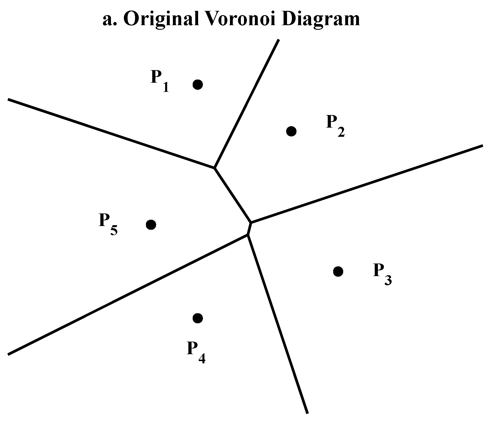
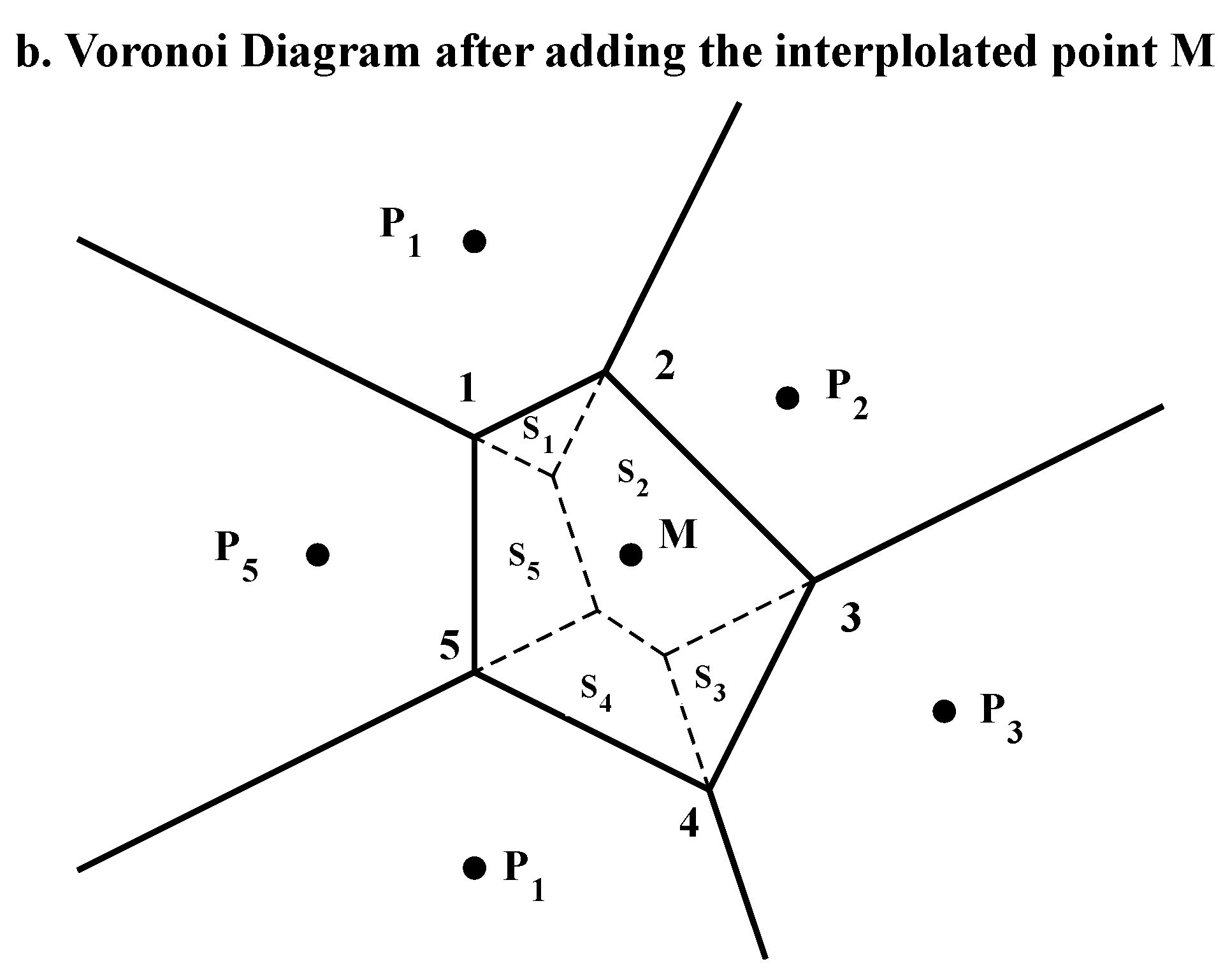
2.3. Natural Neighbor Interpolation

The GPS TEC obtained from GPS data was discrete. To obtain the spatial distribution of GPS TEC in the Maduo and Yangbi seismogenic zones, we introduced the natural neighbor interpolation (NNI) method. NNI is a spatial interpolation method, which has the advantages of fast calculation speed, high precision, and short operation time. It has three useful properties: (1) the value of the original point is not changed after interpolation; (2) the point to be interpolated is only affected by its natural neighbors; and (3) the derivative of the interpolated function is continuous, except for the original point [33].
The NNI calculates its interpolation results according to the contribution of each natural neighbor to the point to be interpolated. Assuming that there are N natural neighbors of interpolated point M, which are P 1 , P 2 , P 3 , …, P N 1 , and P N , the following interpolation formula can be constructed:
f M = i = 1 N ω i f ( P i )
where f(M) is the value of the point M after interpolation, f P i is the value at the natural neighbor P i , and ω i are the weights of P i (i = 1, 2, 3, …, N−1, N).
Assuming that the interpolated point M had five natural neighbors, we generated the Voronoi diagram (Figure 2a) using the five natural neighbors, and then generated the Voronoi diagram (Figure 2b) again after adding the point M. The two Voronoi diagrams intersected and enclosed five polygons (Figure 2b), and ω i = S i / S , where S is the sum of the areas of the five polygons and S i (i = 1, 2, 3, 4, and 5) is the area of polygon S i .

3. Results and Analysis

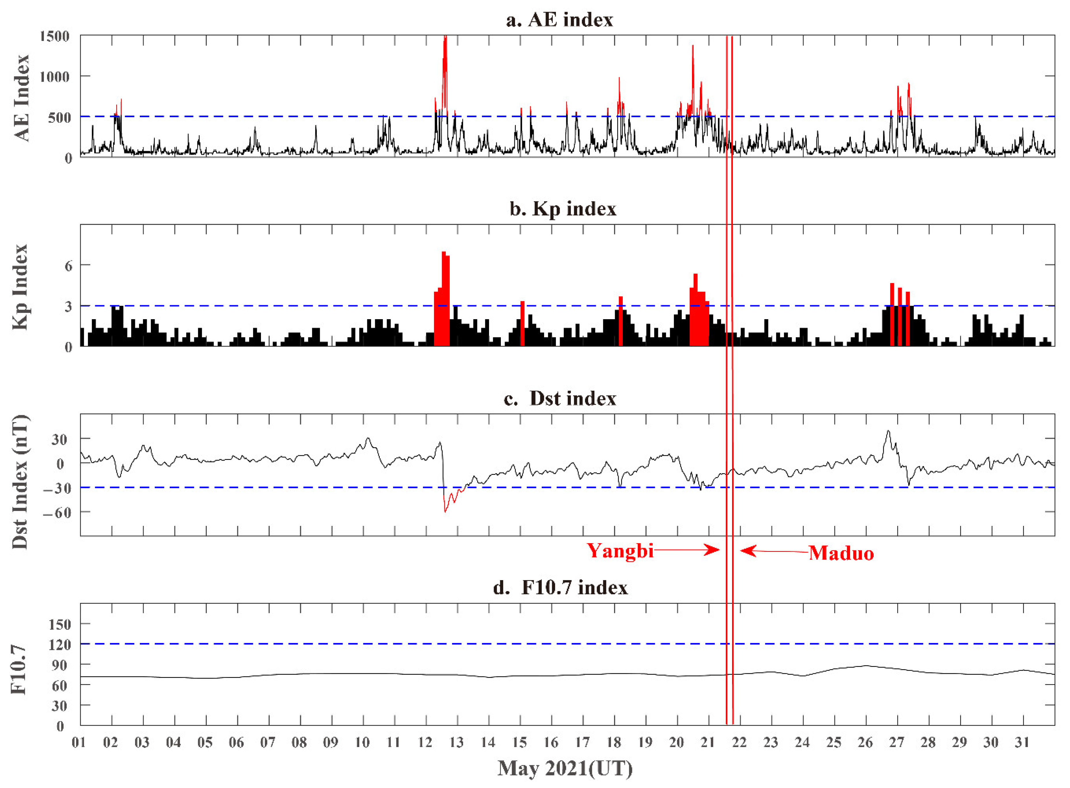
3.1. Solar Activity and Geomagnetic Environment

There are many factors that can cause ionospheric disturbances, such as solar activity, geomagnetic storms, atmospheric waves, and lower atmospheric forcing [27,28,34,35,36,37,38]. Among them, solar activity and geomagnetic storms are important sources of ionospheric disturbance. To ensure that the extracted anomalies were related to earthquakes, it was necessary to examine solar activity level and geomagnetic activity.
In this study, the geomagnetic indices AE, Dst, Kp and the solar activity index F10.7 were selected as the reference for whether the space weather was quiet or not. When geomagnetic activity is strong or solar activity level is high, ionospheric anomalies are likely to be caused by geomagnetic or solar activity. Therefore, we only considered data in relatively quieter geomagnetic conditions (the geomagnetic indices needed to satisfy AE < 500, Kp < 3 and Dst > −30 nt, simultaneously) and solar activity (F10.7 < 120). As Cai et al. [39] pointed out, sometimes geomagnetic disturbances with only Kp < 3 can cause significant impact on the thermosphere and ionosphere.
Figure 3 shows the variations of these indices in May 2021. As shown in Figure 3, F10.7 changes were pretty small and was always lower than 90 in May. This meant the level of solar activity was low, so the influence of solar activity on the ionosphere would have been minimal in May 2021. The AE index exceeded the established threshold on 2 May. The geomagnetic indices (AE, Kp, and Dst) indicated quiet geomagnetic conditions from 3 May to 11 May 2021. A strong geomagnetic storm occurred on 12 May, which lasted until 13 May. There were geomagnetic disturbances on 15, 18, 20, 21, 26, and 27 May. On geomagnetic disturbance days, the ionosphere may have been affected by geomagnetic disturbances.

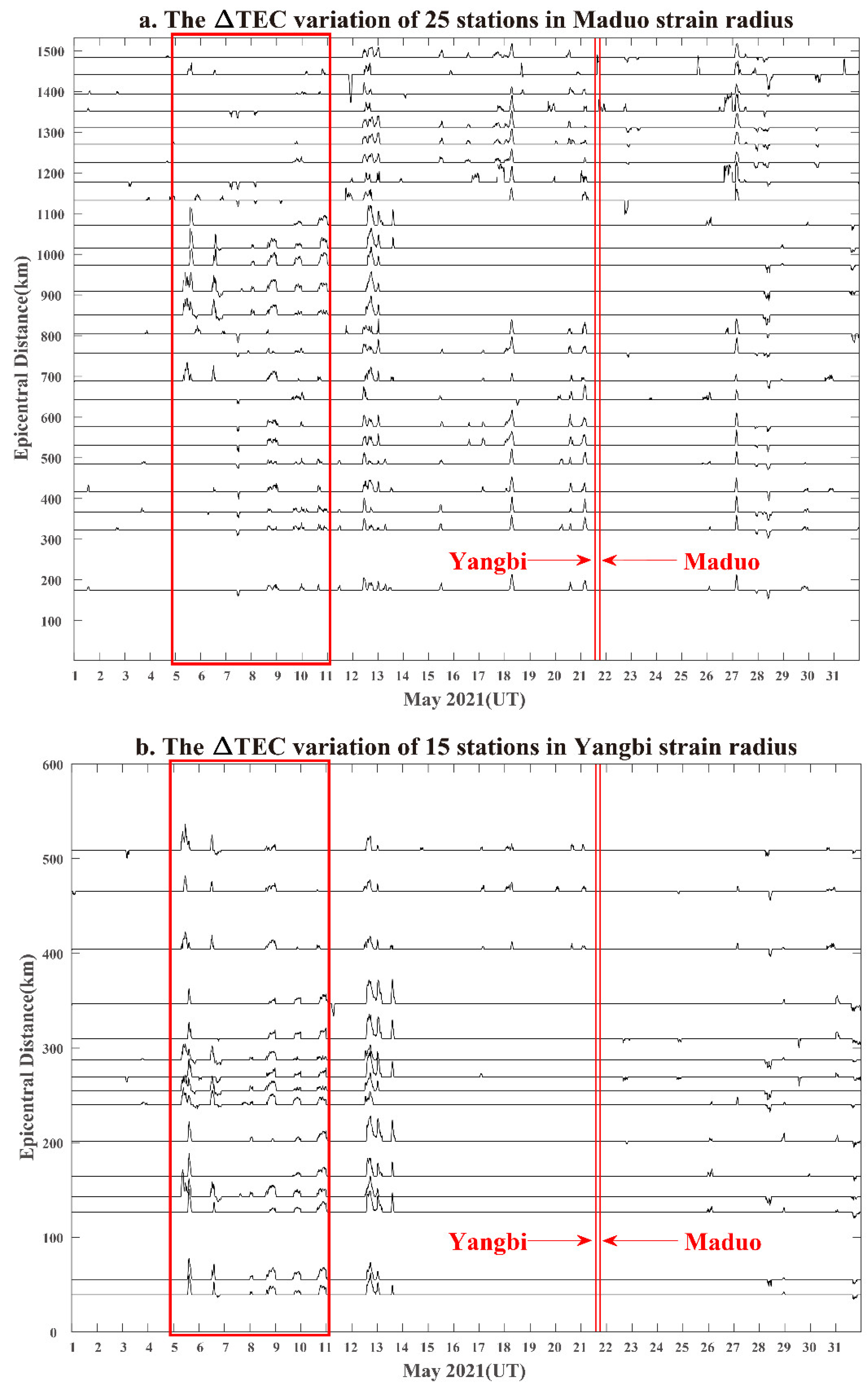
3.2. GPS TEC Time Series Analysis

According to the seismogenic zone of the Maduo and Yangbi earthquakes, there were 72 GPS stations in Maduo and 21 GPS stations in Yangbi from 113 stations. As shown in Figure 1, some stations were almost as far from the epicenter. If data of all stations are displayed, part of the data will overlap in the figure and would not be clearly seen. For a clearer display, we sorted the distances between the stations and the epicenter, then selected the station closest to the epicenter, then selected the next station according to a certain distance interval, up until the farthest station. Finally, we selected 25 and 15 GPS station in Maduo and Yangbi seismogenic zone, respectively. The TEC anomaly of each station was extracted by the interquartile range method. Figure 4 shows the variation of GPS TEC anomalies with time, according to the distance from the station to the epicenter.
Figure 4a shows the GPS TEC anomalies for 25 stations in the Maduo seismogenic zone. Pronounced positive TEC anomalies were extracted at some stations on 5 and 6 May. On 6 May, several stations detected negative TEC anomalies after the positive TEC anomalies. On 7 May, many stations extracted negative TEC anomalies, but they were not particularly obvious compared with the positive TEC anomalies on 5 and 6 May. Many stations detected positive TEC anomalies on 8 to 10 May. All stations detected positive TEC anomalies on 12 May. Some stations detected positive TEC anomalies on 13 May. Positive TEC anomalies were extracted from many stations on 15, 18, 20, and 21 May. After the earthquakes, positive TEC anomalies were extracted on 27 May, and negative TEC anomalies were extracted on 28 and 31 May. Figure 4b shows that almost 15 stations in the Yangbi seismogenic zone were detected positive TEC anomalies on 5 and 6 May. On 6 May, some stations detected negative TEC anomalies after the positive TEC anomalies. Many stations detected positive TEC anomalies on 8 to 10 May. All stations detected positive TEC anomalies on 12 May. Many stations detected positive TEC anomalies on 13 May. The anomaly on the 12 May was very significant. After the earthquake, some stations extracted the negative TEC anomaly on 28 and 31 May.
From Figure 3, we know that there were geomagnetic disturbances on 2, 12, 13, 15, 18, 20, 21, 26, and 27 May. The TEC anomalies of 28 and 31 May occurred after the earthquakes. The anomalies of these magnetic disturbance days may be related to magnetic disturbances, especially the positive TEC anomaly extracted on 12 May, due to the presence of a magnetic storm. In this paper, the TEC anomalies extracted from magnetic disturbance days will not be discussed or analyzed. We were only interested in the TEC anomalies before the earthquake. Thus, the TEC anomalies extracted in the quiet geomagnetic days before the earthquake will be discussed in this study.
Combining Figure 4a,b, pronounced TEC anomalies were detected from 5 to 10 May before the Maduo and Yangbi earthquakes. In the seismogenic zones of Maduo and Yangbi, positive TEC anomalies were extracted on 5 May. Positive and negative TEC anomalies were detected on 6 May. Negative TEC anomalies were detected on 7 May and positive TEC anomalies on 8 to 10 May. The positive TEC anomalies on 5 and 6 May were more significant compared with the negative TEC anomalies on 6 and 7 May and the positive anomalies on 8 to 10 May.

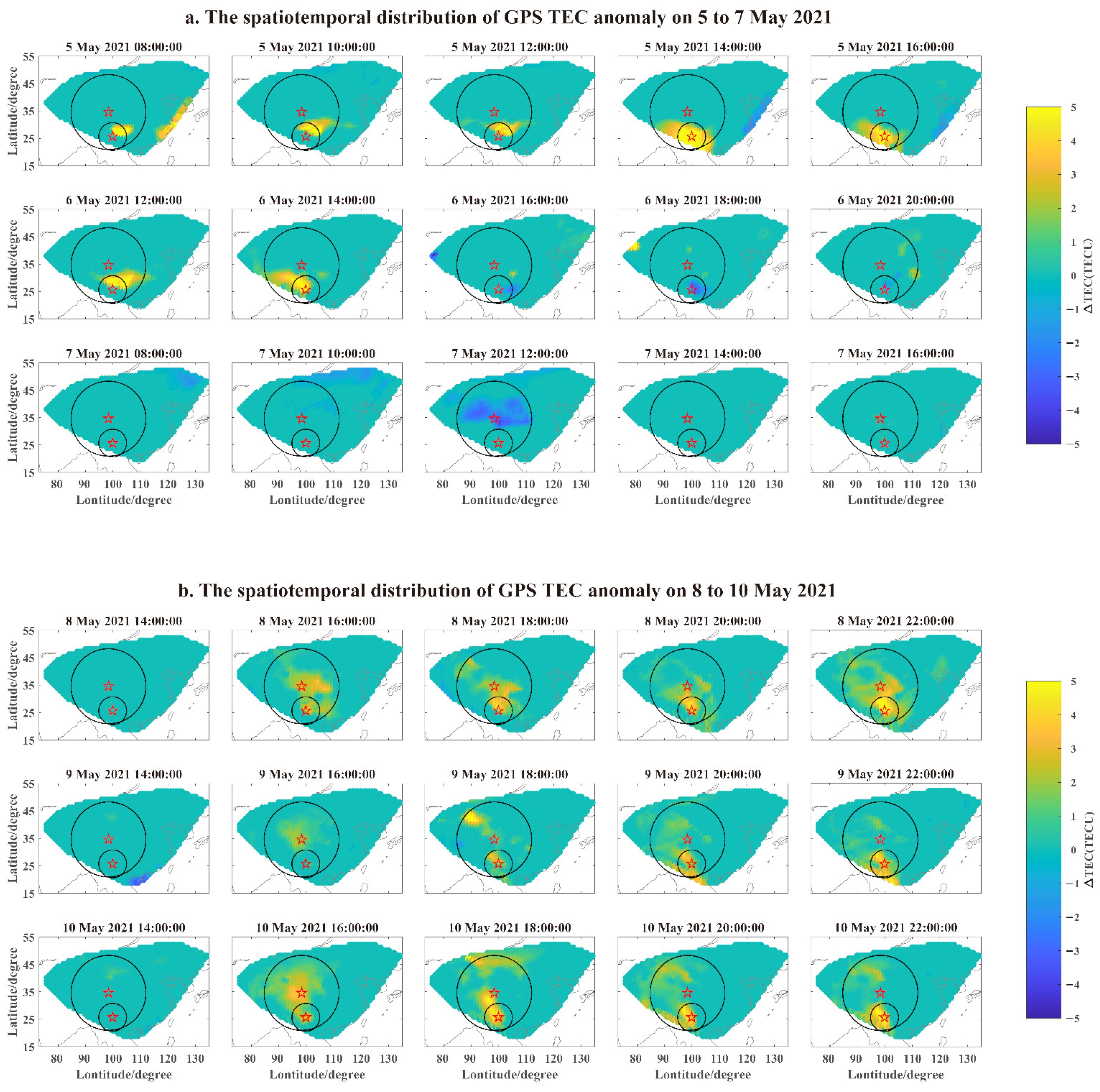
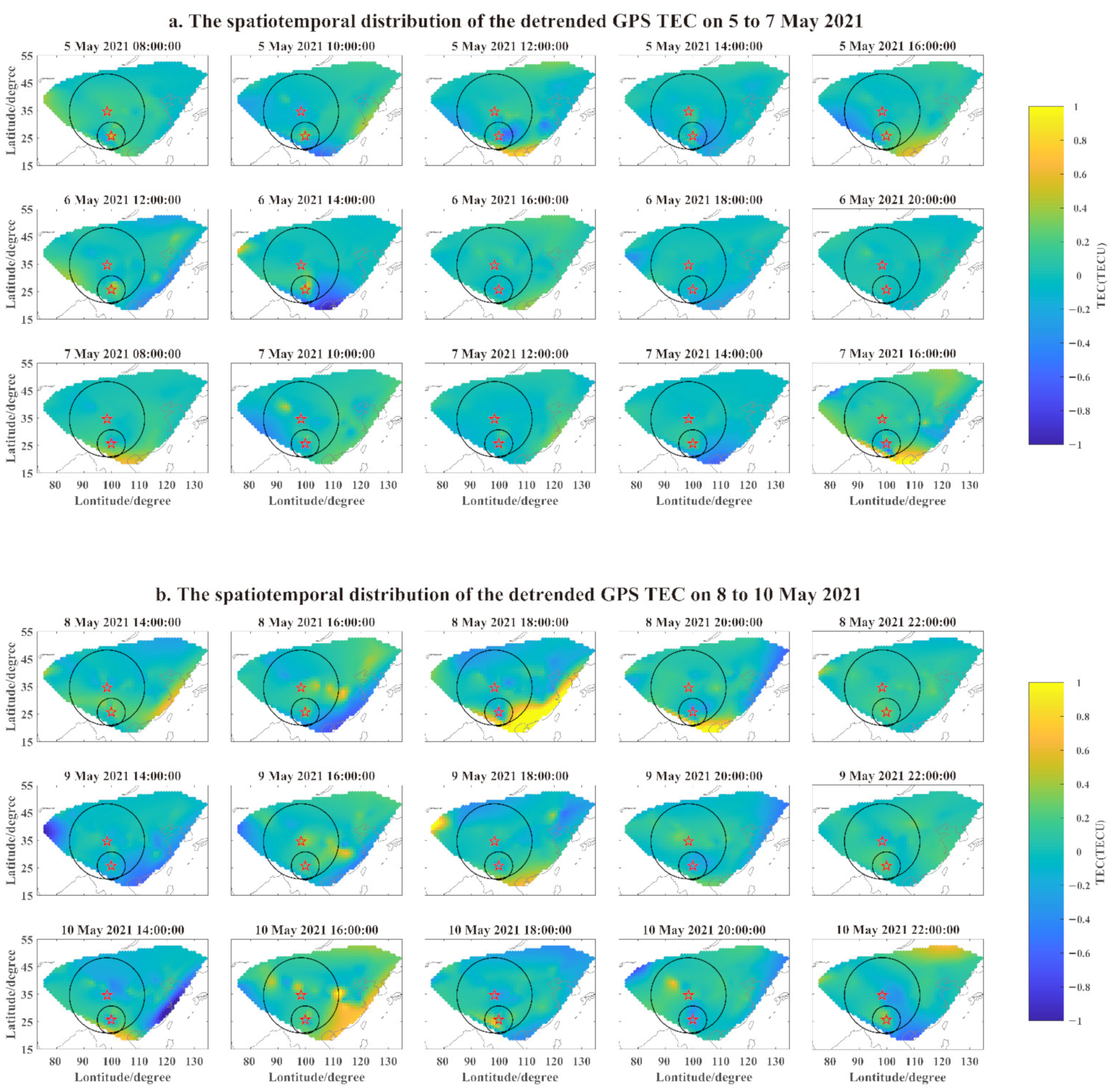
3.3. The Spatiotemporal Distribution of GPS TEC Anomalies

To identify the spatiotemporal distribution characteristics of the TEC anomaly on 5 to 10 May, we obtained GPS TEC grid data with bi-hourly temporal resolution and spatial resolution of 1° along latitude and 1° along longitude by natural neighbor interpolation. The TEC data of 113 GPS stations from CMONOC was used for natural neighbor interpolation. The GPS TEC anomaly grid data was extracted using the sliding quartile method.
Figure 5a shows the spatiotemporal distribution of GPS TEC anomalies on 5 to 7 May. From 08:00 to 16:00 on 5 May, a very significant positive TEC anomaly area was extracted over the Yangbi epicenter and to the southeast of the Maduo epicenter. The anomaly area expanded rapidly in the southwest of the Yangbi epicenter from 12:00 to 14:00 on 5 May. At 12:00 to 14:00 on 6 May, a positive TEC anomaly area was extracted over the Yangbi epicenter and to the southeast of the Maduo epicenter. After that, the positive anomaly area gradually disappeared. From 16:00 to 18:00 on 6 May, a weak negative anomaly area appeared over the Yangbi epicenter and to the southeast of Maduo. At 12:00 on 7 May, a negative anomaly area was detected to the north side of the Yangbi epicenter and over the Maduo epicenter. Figure 5b shows the spatiotemporal distribution of GPS TEC anomalies on 8 to 10 May. The positive TEC anomaly was detected at 16:00–22:00 on 8 to 10 May. Those TEC anomalies were located in the seismogenic zone and around the epicenters of the Yangbi and Maduo earthquakes, indicating that they may have been related to the earthquakes.
Medium scale traveling ionospheric disturbances (MSTID) is a band-like TEC structure that travels in the ionosphere. MSTID was observed in nighttime mid-latitude of the northern hemisphere and tended to travel to the southwest [40]. To show that MSTID was not the source of the TEC anomaly on 5 to 10 May, we used a method similar to Kil and Paxton [41] to detrend the TEC data of the 113 GPS stations with a 1-h window. The spatiotemporal distribution map of the detrended TEC data was calculated by natural neighbor interpolation. We do not find the TEC structure of MSTID in Figure 6a,b. Therefore, the case of MSTID can be excluded.

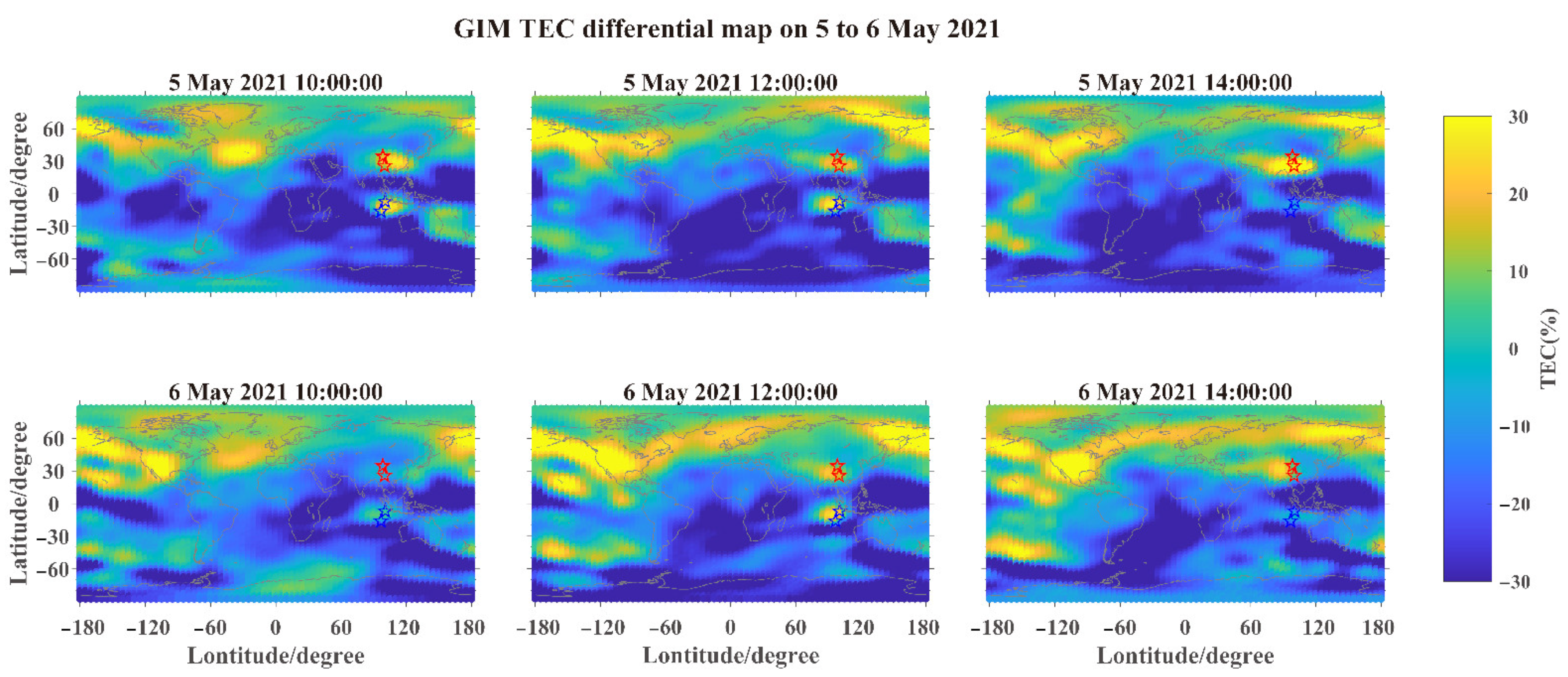
3.4. GIM TEC Differential Map

According to previous studies [13,42], GIM TEC can magnetically record conjugated effects of ionospheric anomalies. We detect conjugated effects by the GIM TEC differential map on 5 to 10 May. The absolute value of TEC at night can be an order of magnitude lower than daytime values. Similar to the method of Pulinets et al. [43], we used percentages to detect small deviations in absolute values at night, which also filtered out daily TEC changes associated with changes in solar UV radiation levels. A GIM TEC differential map was calculated with the formula DTEC = 100(TEC − MTEC)/MTEC, where MTEC is the average TEC value calculated from the 15 previous TEC values for the same moment in time.
By examining the GIM TEC difference map on 5 to 10 May, we only found the conjugation effect at 10:00–12:00 on 5 and 6 May. As shown in Figure 7, we detected TEC enhancement near the Yangbi and Maduo earthquake epicenters and their conjugated points. The conjugation effect was not found on 7 to 10 May. First, as shown in Figure 4a,b, the magnitude of the TEC anomaly on 5 and 6 May was larger than the one on 7 to 10 May. Second, as shown in Figure 7, the conjugation effect was only detected at 10:00–12:00 on 5 and 6 May, whereas the TEC enhancement near the epicenter continued until 14:00. Finally, we know that the GPS TEC anomaly was detected at 12:00 on 7 May and 14:00–22:00 from 8 to 10 May from Figure 6a,b. Thus, the conjugation effect occurred only when the GPS TEC anomaly reached a certain intensity and occurred at a suitable time of the day.

4. Discussions

Based on Figure 1, we can see that the seismogenic zone of the Yangbi earthquake was within the seismogenic zone of the Maduo earthquake, and the occurrence times for the two earthquakes were less than 5 h apart. It was difficult to distinguish whether the possible TEC anomalies were from Yangbi or Maduo or both. Therefore, we took the detected TEC anomalies as the combined effect of the two earthquakes.
In the case of examining solar activity and geomagnetic disturbance days, we detected GPS TEC anomalies on 5 to 10 May using the sliding quartile method. The TEC anomalies were mainly positive. We obtained the spatiotemporal distribution of these TEC anomalies by natural neighbor interpolation. The results showed that the TEC anomalies were mainly around the epicenters of the Maduo and Yangbi earthquakes. Examining these TEC anomalies, we ruled out MSTID. From the GIM TEC differential map, we further found that TEC enhancement occurred in the seismogenic zone and their magnetic conjugated area of the Maduo and Yangbi earthquakes at 10:00–12:00 on 5 and 6 May.
Our results suggest that these TEC anomalies are likely to be associated with the Maduo and Yangbi earthquakes. One possible explanation for this relationship is the lithosphere-atmosphere-ionosphere coupling (LAIC) mechanism. The primary LAIC process is the ionization of the air produced by an increased emanation of radon (and other gases) from the Earth’s crust in the vicinity of an active fault, which leads to changes in the conductivity of the air and latent heat release (increasing air temperature) due to water molecule attachment (condensation) to ions [22]. The variations in air conductivity were the main source of ionospheric anomalies over the seismogenic zone, and the condensation of water vapor was accompanied by latent heat release, which was the main cause for atmospheric thermal anomalies [9]. The seismogenic electric field induced by the change of air conductivity in the seismogenic zone affected the movement of charged particles in the ionosphere through E × B drift, resulting in TEC enhancement or weakening in the earthquake seismogenic zone and the magnetic conjugated area [44]. Thus, the OLR anomaly generated by atmospheric heat accumulation caused the ionospheric response [23].
The TEC enhancement was detected in the seismogenic zone and their magnetic conjugated area of the Maduo and Yangbi earthquakes at 10:00 to 12:00 on 5 and 6 May. The conjugated effect was not observed on 7 to 10 May. In Section 3.4 of this paper, we analyzed the possible reasons. In addition, Zhong et al. [45] observed an increase in radon concentrations from 28 February to 10 March at a measuring point within 254 km from the epicenter of the Maduo earthquake. Based on data from China’s seismo-electromagnetic satellite, Du and Zhang [46] found an enhancement in density and temperature before the earthquakes.
Jing et al. [47] observed OLR anomalies before the earthquake from 1 to 9 May. In particular, the maximum OLR anomalies occurred on 4 May, and then we detected the TEC anomaly on 5 May, indicating an ionospheric response to thermal anomalies, which was consistent with studies by Ouzounov et al. [22,23] These observations can establish some facts about the LAIC process. These anomalies were all detected in the seismogenic zone of the Maduo earthquake, which not only indicated their correlation with the earthquake, but also showed the operation of LAIC. The emission of radon in the seismogenic zone of Maduo earthquake led to changes in air conductivity and release of latent heat. The former affected the ionosphere by inducing a seismogenic electric field. Although we had no electric field observation data, the seismogenic electric field was necessary due to the existence of the magnetic conjugation effect. The latter led to an increase in ground radiative flux through increased ground temperature, resulting in OLR anomalies. The ionosphere responded to OLR anomalies. Based on these results and analysis, we suggested that the Maduo and Yangbi earthquakes affected the ionosphere through the seismogenic electric field and thermal anomalies generated during the LAIC process.

5. Conclusions

In this paper, we analyzed ionospheric perturbations potentially related to the Maduo and Yangbi earthquakes in China on 21 May 2021, using GPS TEC and GIM TEC data. Our results showed that there were the significant TEC anomalies from 5 to 10 May. The geomagnetic activity was relatively quieter during these days, indicating that the influence of geomagnetic activity was weaker. These anomalies were mainly positive, and they were distributed around the epicenter. This suggested that they were related to the earthquakes. Moreover, we detected a magnetic conjugation effect in GIM TEC differential maps on 5 May and 6 May, which was consistent with previous results of ionospheric perturbations associated with earthquakes [13,23]. According to our results and studies by others [45,47], we suggest that the Maduo and Yangbi earthquakes affected the ionosphere through the electric field branch and thermal branch of the LAIC mechanism. Our results provide an example of analyzing ionospheric anomalies based on the LAIC mechanism. However, there is more research needed to support the use of the LAIC mechanism in the earthquake preparation period.

Author Contributions

Conceptualization, X.Z.; data curation, L.D.; investigation, X.Z., L.D. and X.D.; methodology, X.D. and L.D.; writing—original draft, L.D.; writing—review and editing, X.Z. and X.D.; supervision, X.Z. All authors have read and agreed to the published version of the manuscript.

Funding

This research was supported by the Equipment Pre-development Sharing Technology Program (Grant No. 50925020104), National Key R&D Program of China (2018YFC1503506), NSFC project (41674156), ISSI-BJ International Team (2019-33), and the Dragon 5 Cooperation Proposal (#59308).

Institutional Review Board Statement

Not applicable.

Informed Consent Statement

Not applicable.

Data Availability Statement

The data presented in the study are available from the corresponding author by request.

Acknowledgments

The authors are thankful to the CENC, CMONOC, and JPL for providing the earthquake data, GPS data, and GIM TEC data, respectively. The authors are also grateful to the German Research Centre for Geosciences and Kyoto University for providing the solar and geomagnetic activity indexes.

Conflicts of Interest

The authors declare no conflict of interest.

References

  1. Leonard, R.S.; Barnes, R.A. Observation of ionospheric disturbances following the Alaska earthquake. J. Geophys. Res. 1965, 70, 1250–1253. [Google Scholar] [CrossRef]
  2. Calais, E.; Minster, J.B. GPS detection of ionospheric perturbations following the January 17, 1994, Northridge Earthquake. Geophys. Res. Lett. 1995, 22, 1045–1048. [Google Scholar] [CrossRef]
  3. Liu, J.Y.; Chen, Y.I.; Chuo, Y.J.; Tsai, H.F. Variations of ionospheric total electron content during the Chi-Chi earthquake. Geophys. Res. Lett. 2001, 28, 1383–1386. [Google Scholar] [CrossRef] [Green Version]
  4. Liu, J.Y.; Chen, Y.I.; Jhuang, H.K.; Lin, Y.H. Ionospheric foF2 and TEC anomalous days associated with M >= 5.0 earthquakes in Taiwan during 1997–1999. Terr. Atmos. Ocean. Sci. 2004, 15, 371–383. [Google Scholar] [CrossRef] [Green Version]
  5. Liu, J.-Y.; Tsai, Y.-B.; Ma, K.-F.; Chen, Y.-I.; Tsai, H.-F.; Lin, C.-H.; Kamogawa, M.; Lee, C.-P. Ionospheric GPS total electron content (TEC) disturbances triggered by the 26 December 2004 Indian Ocean tsunami. J. Geophys. Res. Space Phys. 2006, 111, 1–4. [Google Scholar] [CrossRef] [Green Version]
  6. Liu, J.Y.; Chen, C.H.; Chen, V.I.; Yang, W.H.; Oyama, K.I.; Kuo, K.W. A statistical study of ionospheric earthquake precursors monitored by using equatorial ionization anomaly of GPS TEC in Taiwan during 2001–2007. J. Asian Earth Sci. 2010, 39, 76–80. [Google Scholar] [CrossRef]
  7. Freund, F. Time-resolved study of charge generation and propagation in igneous rocks. J. Geophys. Res. Solid Earth 2000, 105, 11001–11019. [Google Scholar] [CrossRef] [Green Version]
  8. Freund, F. Charge generation and propagation in igneous rocks. J. Geodyn. 2002, 33, 543–570. [Google Scholar] [CrossRef] [Green Version]
  9. Pulinets, S.; Ouzounov, D. Lithosphere–Atmosphere–Ionosphere Coupling (LAIC) model—An unified concept for earthquake precursors validation. J. Asian Earth Sci. 2011, 41, 371–382. [Google Scholar] [CrossRef]
  10. Molchanov, O.; Fedorov, E.; Schekotov, A.; Gordeev, E.; Chebrov, V.; Surkov, V.; Rozhnoi, A.; Andreevsky, S.; Iudin, D.; Yunga, S.; et al. Lithosphere-atmosphere-ionosphere coupling as governing mechanism for preseismic short-term events in atmosphere and ionosphere. Nat. Hazards Earth Syst. Sci. 2004, 4, 757–767. [Google Scholar] [CrossRef]
  11. Hayakawa, M.; Sue, Y.; Nakamura, T. The effect of earth tides as observed in seismo-electromagnetic precursory signals. Nat. Hazards Earth Syst. Sci. 2009, 9, 1733–1741. [Google Scholar] [CrossRef] [Green Version]
  12. Liu, J.Y.; Chuo, Y.J.; Shan, S.J.; Tsai, Y.B.; Chen, Y.I.; Pulinets, S.A.; Yu, S.B. Pre-earthquake ionospheric anomalies registered by continuous GPS TEC measurements. Ann. Geophys. 2004, 22, 1585–1593. [Google Scholar] [CrossRef] [Green Version]
  13. Liu, J.Y.; Chen, Y.I.; Chen, C.H.; Liu, C.Y.; Chen, C.Y.; Nishihashi, M.; Li, J.Z.; Xia, Y.Q.; Oyama, K.I.; Hattori, K.; et al. Seismoionospheric GPS total electron content anomalies observed before the 12 May 2008 M(w)7.9 Wenchuan earthquake. J. Geophys. Res. Space Phys. 2009, 114, 1–10. [Google Scholar] [CrossRef]
  14. Singh, O.; Chauhan, V.; Singh, V.; Singh, B. Anomalous variation in total electron content (TEC) associated with earthquakes in India during September 2006–November 2007. Phys. Chem. Earth Parts A/B/C 2009, 34, 479–484. [Google Scholar] [CrossRef]
  15. Devbrat, P.; Birbal, S.; Singh, O.P.; Saral Kumar, G.; Karia, S.P.; Pathak, K.N. Study of ionospheric precursors using GPS and GIM-TEC data related to earthquakes occurred on 16 April and 24 September, 2013 in Pakistan region. Adv. Space Res. 2017, 60, 1978–1987. [Google Scholar]
  16. Tariq, M.A.; Shah, M.; Li, Z.; Wang, N.; Shah, M.A.; Iqbal, T.; Liu, L. Lithosphere ionosphere coupling associated with three earthquakes in Pakistan from GPS and GIM TEC. J. Geodyn. 2021, 147, 101860. [Google Scholar] [CrossRef]
  17. Shah, M.; Ahmed, A.; Ehsan, M.; Khan, M.; Tariq, M.A.; Calabia, A.; Rahman, Z.u. Total electron content anomalies associated with earthquakes occurred during 1998–2019. Acta Astronaut. 2020, 175, 268–276. [Google Scholar] [CrossRef]
  18. Freund, F. Pre-earthquake signals: Underlying physical processes. J. Asian Earth Sci. 2011, 41, 383–400. [Google Scholar] [CrossRef]
  19. Freund, F. Earthquake forewarning—A multidisciplinary challenge from the ground up to space. Acta Geophys. 2013, 61, 775–807. [Google Scholar] [CrossRef]
  20. Freund, F. Toward a unified solid state theory for pre-earthquake signals. Acta Geophys. 2010, 58, 719–766. [Google Scholar] [CrossRef]
  21. Shah, M.; Aibar, A.C.; Tariq, M.A.; Ahmed, J.; Ahmed, A. Possible ionosphere and atmosphere precursory analysis related to M-w > 6.0 earthquakes in Japan. Remote Sens. Environ. 2020, 239, 111620. [Google Scholar] [CrossRef]
  22. Ouzounov, D.; Pulinets, S.; Romanov, A.; Romanov, A.; Tsybulya, K.; Davidenko, D.; Kafatos, M.; Taylor, P. Atmosphere-ionosphere response to the M9 Tohoku earthquake revealed by multi-instrument space-borne and ground observations: Preliminary results. Earthq. Sci. 2011, 24, 557–564. [Google Scholar] [CrossRef] [Green Version]
  23. Ouzounov, D.; Pulinets, S.; Davidenko, D.; Rozhnoi, A.; Solovieva, M.; Fedun, V.; Dwivedi, B.; Rybin, A.; Kafatos, M.; Taylor, P. Transient effects in atmosphere and ionosphere preceding the 2015 M7. 8 and M7. 3 Gorkha–Nepal earthquakes. Front. Earth Sci. 2021, 9, 757358. [Google Scholar] [CrossRef]
  24. Parrot, M.; Tramutoli, V.; Liu, T.J.Y.; Pulinets, S.; Ouzounov, D.; Genzano, N.; Lisi, M.; Hattori, K.; Namgaladze, A. Atmospheric and ionospheric coupling phenomena associated with large earthquakes. Eur. Phys. J. Spec. Top. 2021, 230, 197–225. [Google Scholar] [CrossRef]
  25. Pulinets, S.A. Physical mechanism of the vertical electric field generation over active tectonic faults. Adv. Space Res. 2009, 44, 767–773. [Google Scholar] [CrossRef]
  26. Pulinets, S.; Khachikyan, G. The Global Electric Circuit and Global Seismicity. Geosciences 2021, 11, 491. [Google Scholar] [CrossRef]
  27. Thomas, E.; Baker, J.; Ruohoniemi, J.; Coster, A.; Zhang, S.R. The geomagnetic storm time response of GPS total electron content in the North American sector. J. Geophys. Res. Space Phys. 2016, 121, 1744–1759. [Google Scholar] [CrossRef] [Green Version]
  28. Afraimovich, E.; Astafyeva, E.; Oinats, A.; Yasukevich, Y.V.; Zhivetiev, I. Global electron content: A new conception to track solar activity. In Proceedings of the 3rd European Space Weather Week (ESWW 2006), Brussels, Belgium, 13–17 November 2006; pp. 335–344. [Google Scholar]
  29. Klobuchar, J.A. Ionospheric Time-Delay Algorithms for Single-Frequency GPS Users. IEEE Trans. Aerosp. Electron. Syst. 1987, AES-23, 325–331. [Google Scholar] [CrossRef]
  30. Jin, S.; Jin, R.; Li, J.H. Pattern and evolution of seismo-ionospheric disturbances following the 2011 Tohoku earthquakes from GPS observations. J. Geophys. Res.-Space Phys. 2014, 119, 7914–7927. [Google Scholar] [CrossRef] [Green Version]
  31. Dobrovolsky, I.; Zubkov, S.; Miachkin, V. Estimation of the size of earthquake preparation zones. Pure Appl. Geophys. 1979, 117, 1025–1044. [Google Scholar] [CrossRef]
  32. Liu, L.; Yao, Y.; Kong, J. Study on Ionospheric TEC Anomaly Before Nepal Earthquake. J. Geomat. 2016, 41, 13–17. [Google Scholar] [CrossRef]
  33. Malcolm, S.; Jean, B.; Herbert, M.Q. Geophysical parametrization and interpolation of irregular data using natural neighbours. Geophys. J. Int. 1995, 122, 837–857. [Google Scholar]
  34. Pulinets, S.; Davidenko, D. Ionospheric precursors of earthquakes and global electric circuit. Adv. Space Res. 2014, 53, 709–723. [Google Scholar] [CrossRef]
  35. Namgaladze, A.A. Earthquakes and global electrical circuit. Russ. J. Phys. Chem. B 2013, 7, 589–593. [Google Scholar] [CrossRef]
  36. Gan, Q.; Yue, J.; Chang, L.C.; Wang, W.B.; Zhang, S.D.; Du, J. Observations of thermosphere and ionosphere changes due to the dissipative 6.5-day wave in the lower thermosphere. Ann. Geophys. 2015, 33, 913–922. [Google Scholar] [CrossRef] [Green Version]
  37. Liu, Y.; Zhou, C.; Zhang, X.; Liang, R.; Liu, X.; Zhao, Z. GNSS observations of ionospheric disturbances in response to the underground nuclear explosion in North Korea. Chin. J. Geophys.-Chin. Ed. 2020, 63, 1308–1317. [Google Scholar] [CrossRef]
  38. Pulinets, S.; Davidenko, D.; Pulinets, M. Atmosphere-ionosphere coupling induced by volcanoes eruption and dust storms and role of GEC as the agent of geospheres interaction. Adv. Space Res. 2022, 69, 4319–4334. [Google Scholar] [CrossRef]
  39. Cai, X.; Burns, A.G.; Wang, W.; Qian, L.; Solomon, S.C.; Eastes, R.W.; Pedatella, N.; Daniell, R.E.; McClintock, W.E. The Two-Dimensional Evolution of Thermospheric ∑O/N2 Response to Weak Geomagnetic Activity During Solar-Minimum Observed by GOLD. Geophys. Res. Lett. 2020, 47, e2020GL088838. [Google Scholar] [CrossRef]
  40. Saito, A.; Fukao, S.; Miyazaki, S. High resolution mapping of TEC perturbations with the GSI GPS Network over Japan. Geophys. Res. Lett. 1998, 25, 3079–3082. [Google Scholar] [CrossRef]
  41. Kil, H.; Paxton, L.J. Global Distribution of Nighttime Medium-Scale Traveling Ionospheric Disturbances Seen by Swarm Satellites. Geophys. Res. Lett. 2017, 44, 9176–9182. [Google Scholar] [CrossRef]
  42. Pulinets, S.A.; Bondur, V.G.; Tsidilina, M.N.; Gaponova, M.V. Verification of the concept of seismoionospheric coupling under quiet heliogeomagnetic conditions, using the Wenchuan (China) earthquake of May 12, 2008, as an example. Geomagn. Aeron. 2010, 50, 231–242. [Google Scholar] [CrossRef]
  43. Pulinets, S.; Krankowski, A.; Hernandez-Pajares, M.; Marra, S.; Cherniak, I.; Zakharenkova, I.; Rothkaehl, H.; Kotulak, K.; Davidenko, D.; Blaszkiewicz, L.; et al. Ionosphere Sounding for Pre-seismic Anomalies Identification (INSPIRE): Results of the Project and Perspectives for the Short-Term Earthquake Forecast. Front. Earth Sci. 2021, 9, 1–16. [Google Scholar] [CrossRef]
  44. Pulinets, S.; Ouzounov, D.; Karelin, A.; Davidenko, D. Lithosphere-Atmosphere-Ionosphere-Magnetosphere Coupling-A Concept for Pre-Earthquake Signals Generation: A Multidisciplinary Approach to Earthquake Prediction Studies; AGU: Washington, DC, USA; Wiley: Hoboken, NJ, USA, 2018. [Google Scholar]
  45. Zhong, J.; Wang, B.; Zhou, Z.; Yan, R. Analysis on Anomaly Characteristics of Underground Fluid before 2021 Maduo MS7.4 Earthquake in Qinghai Province. Earthq. Res. China 2021, 37, 574–585, (In Chinese with an English abstract). [Google Scholar]
  46. Du, X.; Zhang, X. Ionospheric Disturbances Possibly Associated with Yangbi Ms6.4 and Maduo Ms7.4 Earthquakes in China from China Seismo Electromagnetic Satellite. Atmosphere 2022, 13, 438. [Google Scholar] [CrossRef]
  47. Jing, F.; Zhang, L.; Singh, R.P. Pronounced Changes in Thermal Signals Associated with the Madoi (China) M 7.3 Earthquake from Passive Microwave and Infrared Satellite Data. Remote Sens. 2022, 14, 2539. [Google Scholar] [CrossRef]
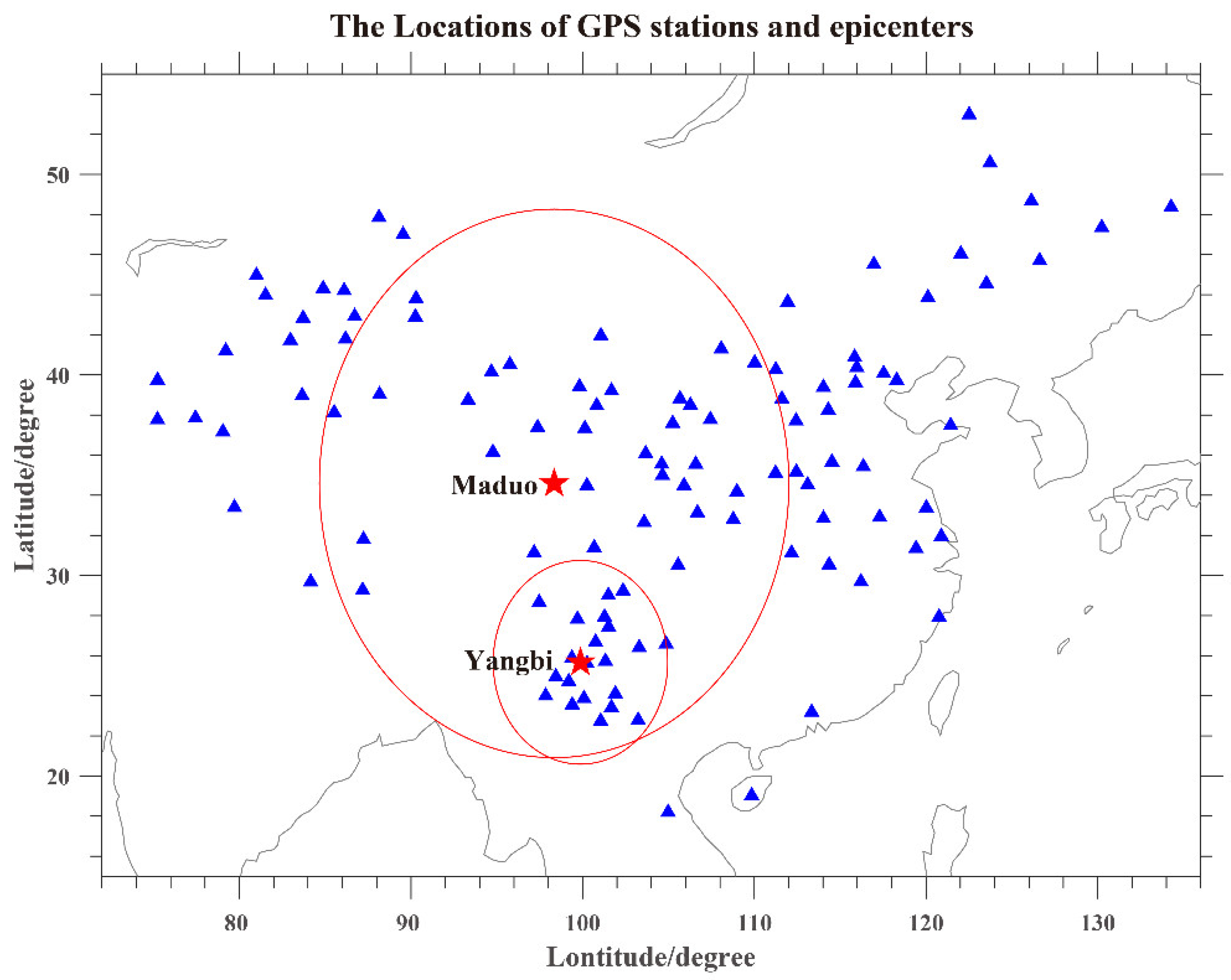
Figure 1. The locations of GPS observing stations and epicenters. The red pentagrams represented the epicenters of Maduo and Yangbi, the blue triangles represent the GPS observation stations, and the red circles represent the seismogenic zone drawn according to the strain radius. Obviously, the seismogenic zone of Yangbi was almost in the seismogenic zone of Maduo.
Atmosphere 13 01725 g001
Figure 2. Voronoi diagram. The Voronoi diagrams of subfigure (a,b) were the results before and after adding the interpolated point M, respectively. The points of P i (i = 1, 2, 3, 4, and 5) were the natural neighbors of point M, and S i (i = 1, 2, 3, 4, and 5) was the area of the polygon corresponding to P i .
Atmosphere 13 01725 g002aAtmosphere 13 01725 g002b
Figure 3. The four panels showed the variations of AE, Kp, and Dst indices and F10.7 solar flux in May 2021, respectively. Red data represents exceeding the threshold, blue dotted line represents the threshold line. The two red vertical lines represent the time of the earthquakes.
Atmosphere 13 01725 g003
Figure 4. The variations of TEC anomalies for May 2021, according to the distance from the GPS station to the epicenter. The epicentral distances of subfigure (a,b) are GPS Δ TEC plus the distance from GPS stations to the epicenters of Maduo and Yangbi, respectively. The horizontal axis represent time. The two red vertical lines represent the time of the earthquakes.
Atmosphere 13 01725 g004
Figure 5. The spatiotemporal distribution of GPS TEC anomalies. The subfigures (a,b) represent the spatiotemporal distribution of GPS TEC anomaly for 5 to 7 May and 8 to 10 May, respectively. The red pentagrams represent the epicenters of the earthquakes; Maduo was to the north of Yangbi. The two black circles represent the seismogenic zones of the earthquakes.
Atmosphere 13 01725 g005
Figure 6. The spatiotemporal distribution map of the detrended GPS TEC data. The subfigures (a,b) represent the spatiotemporal distribution of the detrended GPS TEC data for 5 to 7 May and 8 May to 10 May, respectively. The red pentagrams represent the epicenters of the earthquakes; Maduo was to the north of Yangbi. The two black circles represent the seismogenic zones of the earthquakes.
Atmosphere 13 01725 g006
Figure 7. GIM TEC differential map on 5 and 6 May. The red pentagrams represent the epicenters of Maduo and Yangbi earthquakes; Maduo was to the north side of Yangbi. The blue pentagrams represent the magnetic conjugated points of epicenters.
Atmosphere 13 01725 g007
Table 1. Details of Maduo and Yangbi earthquakes.
Sr.
No.
MagnitudeTime (UT)LatitudeLongitudeDepth (km)RegionsStrain Radius (km)
16.421 May 2021 13:48:3425.6799.878Yangbi564
27.421 May 2021 18:04:1134.5998.3417Maduo1520
Publisher’s Note: MDPI stays neutral with regard to jurisdictional claims in published maps and institutional affiliations.

