Seminal Stacked Long Short-Term Memory (SS-LSTM) Model for Forecasting Particulate Matter (PM2.5 and PM10)

Abstract

With increased industrialization and urbanization, sustainable smart environments are becoming more concerned with particulate matter (PM) forecasts that are based on artificial intelligence (AI) techniques. The intercorrelation between multiple pollutant components and the extremely volatile PM pattern changes are the key impediments to effective prediction. For accurate PM forecasting with the benefit of federated learning, a new architecture incorporating seminal stacked long short-term memory networks (SS-LSTM) is presented in this research. The historical data are analyzed using SS-LSTM to reveal the location-aware behavior of PM, and a new prediction model is generated that takes into account the most prevalent pollutants and weather conditions. The stacking of LSTM units adds hierarchical levels of knowledge that help to tune the forecast model with the most appropriate weighting to the external features that contribute toward PM. The suggested SS-LSTM model is compared with traditional machine learning approaches and deep learning models to see how well it performs in predicting PM2.5 and PM10. The suggested strategy outperforms all other models tested in experiments carried out for the data collected from Delhi in India.

1. Introduction

In recent years, greater emphasis has been paid worldwide to air quality regulation as one of the most critical and long-standing concerns of human civilization [1]. People’s health, economic well-being, and civilizational progress are negatively influenced by air pollution [2]. Particulate matter (PM) is one of the major factors monitored for the air quality index (AQI), along with four other primary pollutants that are: ozone (O₃), carbon monoxide (CO), nitrogen dioxide (NO₂) and sulfur dioxide (SO₂) [3]. PM2.5 concentration readings taken at US embassies and consulates in five major Indian cities were examined for changes, trends, and exceedances [4]. Over the course of the last few years, New Delhi, India’s capital city, has seen frequent and severe pollution incidents. The origins of such high pollutant concentrations are still poorly understood, which makes it difficult to devise effective control techniques. Agriculture plays a larger role in emitting the secondary inorganic aerosols that are present in PM, as do road traffic and open burning, all of which contribute more to aerosols in PM. The primary source of PM2.5 emissions is derived from the residential suburbs [5].

The need to predict and avoid air pollution problems is enhanced by determining the exact PM concentration. Measures such as giving travel warnings, offering self-protection tips, or restructuring transport usage output may all be made more effective with more accurate PM forecasts. This kind of instruction is essential to secure social well-being and environmental preservation. Internal variables, such as industrial output, energy extraction, and transportation make the PM level shift upward, but this is difficult to predict [6]. Particulate matter has a huge impact on the AQI. The AQI is calculated in a number of different ways, some of which are country-specific, while others are tied to the particular subindex of pollutants that are most prevalent in that location [7].

PM has adverse effects on human health, which are increasing as the years pass. The epidemiological study, animal toxicology test, and human clinical observation of PM10 reveal that it has apparent and direct hazardous effects on human health, and may cause severe damage to the respiratory system, blood system, immunological system, and endocrine system [8,9]. Meanwhile, the degree of exposure to PM10 concentrations is also crucial and its impact is huge. When the mass concentration of PM10 exceeds 100 μg/m³, the mortality rate is 11% higher than when the mass concentration is less than 50 μg/m³. Some studies assess the source and accumulation of PM using the precipitation of other substances in the environment. All aerosol tracking flow models presume that future aerosol and aerosol precursor emissions will be drastically reduced. There is ample evidence that, historically, aerosols have influenced tropical precipitation, but there is no scope for a decrease in the aerosol particles [10]. Therefore, a correct and prompt forecast of PM2.5 and PM10 is of the utmost importance in terms of both the study of climate and the advancement of socioeconomic conditions [11].

Statistical approaches have been applied in air pollution forecasts since the 1930s, not only in recent years; they have steadily evolved as a research trend due to their benefits of high efficiency and accuracy in predicting the levels of aerosol particles [12]. Poor air quality demonstrably harms human health; therefore, anticipating pollution levels is critical for public safety. Some studies in the literature have suggested that this approach is inspired by recent deep-learning time series prediction advances. Pollution prediction incorporates an attention layer that captures the recursive temporal connection of air quality data [13]. Combining multi-step forecast results based on uncertainty measures improves accuracy. Enriching the Bayesian-based deep learning model with domain-specific information reduces prediction errors while integrating several forecast approaches enhances forecast precision [14].

To improve our deep-learning model’s interpretability and prediction accuracy, several domain-specific parameters are used, including basin optimization with multivariate time-bound air-quality prediction [15,16]. Experts’ interest in PM2.5 forecasting has increased in recent years, as a result of a noticeable decline in general health compared to past decades. There are primarily two kinds of PM2.5 forecasting approaches in the literature: quantitative modeling and statistical modeling. The numerical modeling approach uses numerical calculations to create models, depending on physical and chemical properties. The prediction is carried out by analyzing the distributions of fine particulate matter within the atmosphere and applying the conservation equations [17]. The statistical modeling technique is typically more practical, yielding systematic forecast results. It does, however, need thorough and exact information on local climate, mountain formations, and the distribution of major pollution sources [18].

The majority of predictive methods are also known as data-driven techniques. These data-driven approaches fit the target data by using numerous samples to continuously refine and approximate the true model. The long short-term memory network is a cutting-edge data-driven strategy [19]. A long short-term memory (LSTM) deep learning-based aggregated LSTM model (ALSTM) is proposed, wherein data from the local air quality measurement station, the station for neighboring industrial regions, and the station for external pollution sources are combined. To increase the forecast precision, the model combines the LSTM models into a predictive model for early predictions, related to external pollution sources and data from adjacent air quality monitoring stations [20]. LSTM can accomplish challenges that traditional recurrent neural network (RNN) learning algorithms could not surmount. It is possible to find a flaw in LSTM networks handling continuous input channels that are not divided into subsequences with clearly defined endpoints. Too much of a delay in resetting the state may cause the connection to fail, which creates the “memory vanish” state in the LSTM model. An adaptive “forget gate” in an LSTM cell may adapt to reset itself at the correct moments, freeing internal resources. Some examples address the benchmark issues in LSTM and make it better than other RNN algorithms, although all algorithms fail to tackle these issues. However, an LSTM with predefined forget gates solves these algorithms elegantly [21].

A prediction model has been developed, based on single value decomposition (SVD) and bidirectional LSTM. The monitoring signal is the cutting force of the bidirectional LSTM, which back-traverses the LSTM unit to obtain information on the behaviour of pollutants in the past. A Hankel matrix is used to reconstruct the basic cutting parameter tuning, then an SVD is used to retrieve the actual characteristics. Then, using the bidirectional LSTM, the current tool wear forecast value is derived using SVD characteristics from the current sample period and the preceding four sampling periods [22]. In certain research works, the non-periodic PM2.5 signal has also been decomposed in the spectral domain using variational mode decomposition (VMD). Decaying the complex signal into several harmonic sub-series reduces its frequency domain complexity [23,24].

The data for this research were collected from the Central Pollution Control Board (CPCB), India. The CPCB is a governing body that functions under the Ministry of Environment and Forests of the Provision of the Environment. Delhi was chosen for the experiment, along with its neighboring monitoring stations. It was selected based on population density and as a way to capture the huge meteorological changes seen in the capital of the country. A novel SS-LSTM model is proposed and is compared with traditional approaches using evaluation metrics, such as MAE, MAPE, and RMSE. Predicting PM2.5 and PM10 is superior and accurate compared to the existing approaches. All traditional approaches are built via the aggregation of LSTM units, with the forget gates tuned. The modern stacking of LSTM helps in addressing the problem of forecasting for smaller time targets. The level of importance in tuning the LSTM unit stacking mechanism provides a hierarchy that scales the entire network to build an efficient forecasting model.

In recent decades, the haze created by industry has exacerbated environmental pollution. This haze worsens when the pollution in the particular location is predominantly of particulate matter. PM2.5 comprises harmful airborne particles sized 2.5 μm or less. This size of particle is harmful to health, primarily in the lungs; due to its minute size, it enters the respiratory tract easily. Worldwide, 90% of people inhale toxic air that exceeds WHO standards [25]. PM2.5 air quality in cities must be tackled promptly; hence, PM2.5 prediction is crucial for smart city development. PM2.5 propagation is affected by meteorological factors, such as wind speed and wind direction, making prediction difficult. Wind direction and speed measurements are unpredictable and vary frequently [26,27]. Researchers have developed a number of different ways of predicting PM2.5 levels based on statistical models and methods of machine learning. Deep neural networks have only recently been adopted by the academic community for the purpose of predicting pollutant concentrations. Deep learning may be able to address issues because it makes use of a greater number of layers and more comprehensive data sets, and also processes all of the layers concurrently to generate more accurate answers [28].

The more conventional statistical approaches have seen a great breadth of application in the processing of air quality forecasting issues. The strategy of gaining knowledge from past events is a significant inspiration for these strategies, which are founded on it. The autoregressive moving average, often known as ARMA, is one of the most well-known statistical models that has been used for predicting air quality [29]. It is more likely that an autoregressive integrated moving average (ARIMA) model will be employed for analyzing the trend or pattern behind the pollutants [30,31]. As artificial intelligence with big data continues to advance, techniques of prediction that are based on machine learning algorithms are becoming more widespread. Because the use of these kinds of models does not need a vast knowledge of the physical or chemical characteristics of air contaminants. Multiple linear regression (MLR), sometimes known as random forest (RF), is one of the most widely used machine learning algorithms [32].

Support vector regression (SVR) methods have been shown to be an effective method for resolving time series issues in a variety of research domains. There has not been a significant amount of research performed on the use of SVR models for the forecasting of concentrations of air pollutants. Data preparation processes and the parameter estimation of SVR models both have the potential to have a significant impact on the accuracy of forecasts [33]. Forecasting the practical quality of the air is made more difficult by the use of inadequate data in the training phase. It is possible to significantly improve the prediction performance, not only in the case of an artificial neural network (ANN) but also in a support vector machine (SVM), by amending the standard error of the traditional methods [34]. This is accomplished through the use of a combination ANN and a blended SVM. Ensemble approaches offer new insights for temporal predictions.

Early research works used ANN or SVM prediction with past data and exogenous inputs, such as variables related to the weather. Later, a forecasting model was employed to make adjustments to the forecasting objective, using the information that had been left over from the previous stage’s error term. Some conventional approaches made the model more precise to forecast the target horizons. Valuable residual knowledge on an imperfect input variable condition is used in such a way that it offers an adequate and legitimate approach [35]. To consider the many nonlinear relationships between the intensity of air contaminants and other important aspects of the weather, and to provide accurate forecasts of air pollution in a variety of research regions, a number of different ANN architectures, such as neuro-fuzzy neural networks (NFNN), have been created [36].

2. Materials and Methods

2.1. Legacy Models for Forecasting with Neural Network and LSTM

Deep learning techniques, including the recurrent neural network (RNN) and its variants, have proliferated in tandem with the rise of interest in utilizing AI techniques. These algorithms are used to train neural network models that leverage by tuning the hyperparameters in an efficient manner. In the field of air-quality forecasting, the LSTM model is one of the most popular options [37]. The RNN processes climate sequence data, each piece of data is linked to one record of the previous time target. This approach for establishing the connection from one output to the next input creates an advanced forecast model; for example, the temperature of that particular area may be an active parameter contributing toward the particulate matter. In climate data such as temperature prediction, day-to-day temperatures are related; past data will provide insight to help forecast better in the future. This can generate many sequences from continuous data using time periods; the relationship between sequences can be determined from the various sequences. Rainy weeks and PM10 are easily correlated with the PM2.5 data. Rain washes air pollutants out of the air and down to the ground, reducing PM2.5 levels. When the PM10 levels are high, PM2.5 levels rise automatically, even though PM2.5 and PM10 are not the same. PM10 comprises a proportion of PM2.5 in that location; the value depends upon the aerosol chemistry in that location. RNN will help us to determine if time series data are correlated [38]. A comparison of the LSTM with the DAE was used to predict the PM concentration at Seoul, South Korea, along with the historic meteorological parameters. It was clear from this comparison that the LSTM predictive algorithm was more reliable than the DAE model [39].

The study of the ways in which dangerous contaminants can have an effect on human health is a large field of inquiry. It is the primary responsibility of any governing authority to either prevent or limit pollution, as well as to monitor its levels. Comparisons and contrasts have been made between a number of different computer models, ranging from statistics and machine learning algorithms to deep learning, in order to demonstrate how accurate the forecasting of air quality requirements has been up to this point. Many regions of the world still do not have their levels of pollutants under control, due to the fact that there are many different causes and reasons for this problem. By utilizing a reversible long short-term memory model, the method that has been suggested makes an effort to anticipate the PM2.5 pollutant levels, one of the more harmful pollutants that are responsible for triggering diseases all over the world [40]. RNNs are a strong form of artificial neural network that is most frequently utilized for solving challenges involving time series forecasting. An RNN is able to retain its own memory and recall information from events in the past that may be used to make predictions about the future. On the other hand, RNNs commonly experience disappearing and bursting gradients, which cause the model’s learning process to become excessively sluggish [18,41].

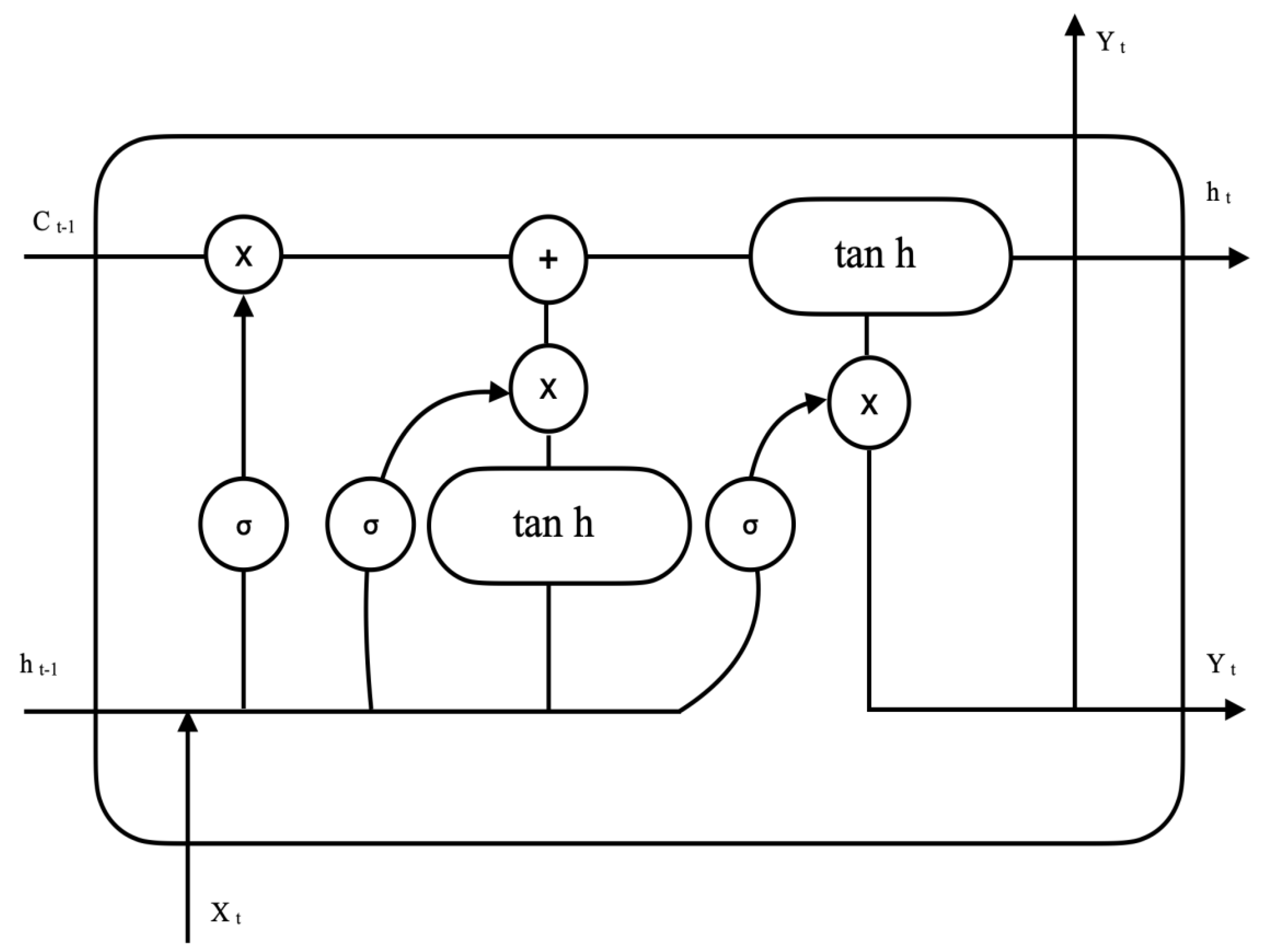
LSTMs are capable of learning from data that are spaced out over a significant amount of time and have a longer memory than other types of neural networks. An LSTM comprises 3 gates: an input gate, which selects whether to accept or not accept new information as input; a forget gate, which deletes knowledge that is deemed to be unimportant; and an output gate, which determines what information should be produced for output. These three gates are analogous gates that are based on the sigmoid function, which operates on values in the range from 0 to 1. LSTM is mostly used to handle the problem of processing sequence data, wherein each data segment is correlated with the previous segment that came before, as shown in Figure 1. The message of neurons from the previous instant will be coupled to the signal neuron of the present moment, and the problem of the LSTM’s dependency on the data over the long term may be overcome by employing the gates that are included inside the LSTM. For the purposes of PM2.5 forecasting, a hybrid deep learning model-based framework can be employed [4]. The predicted accuracy of PM2.5 on a local, regional, or even continental scale may be improved using a variety of different methodologies, including meteorological, geographic, land use, and satellite data. Deep learning techniques have become an active research area in recent years as a result of the growth of big data technology. These techniques are used to predict air quality; the frequent models that are broadly used include fully connected layers of RNN and their variants. The long short-term memory unit, or LSTM, is a futuristic RNN model that is utilized in the process of air quality prediction [42].

2.2. Proposed Methodology

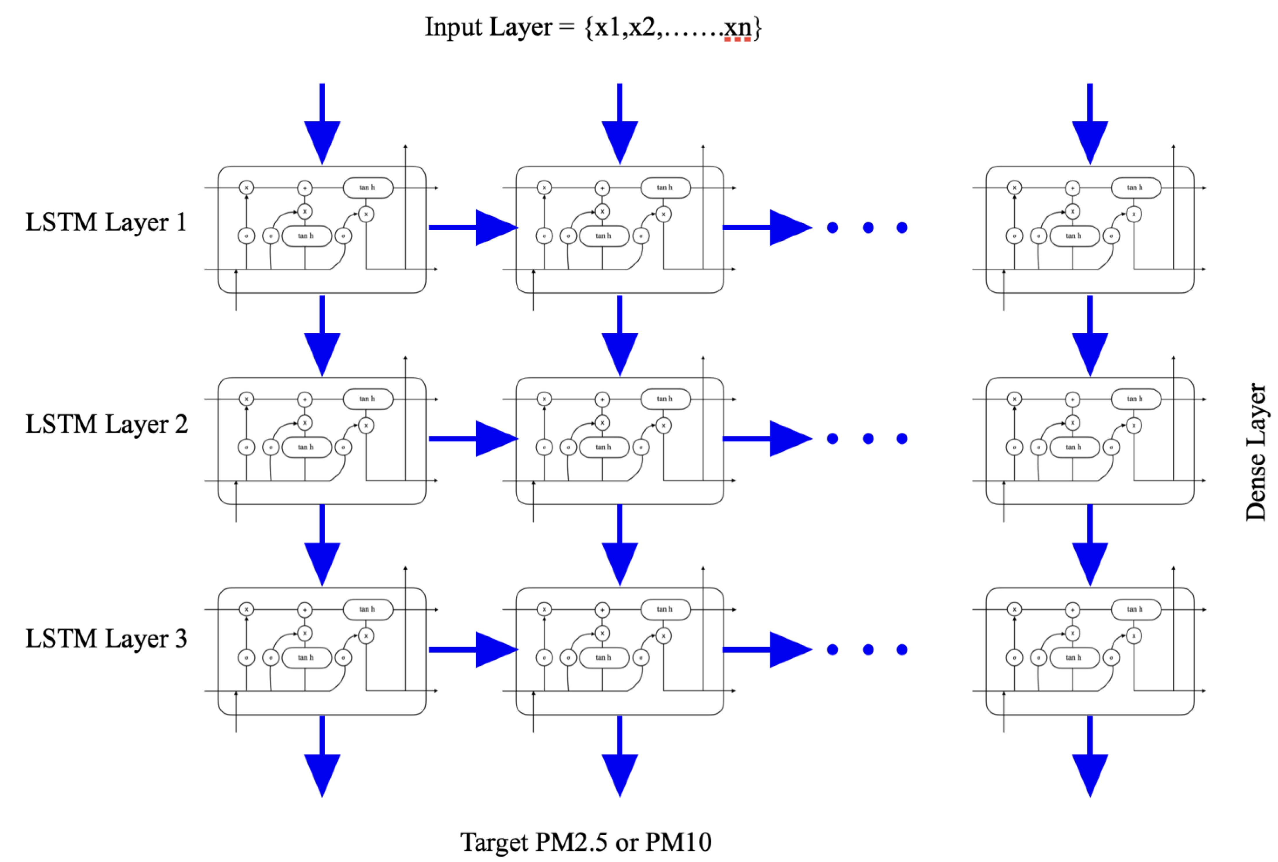
Stacking LSTMs has matured into a reliable method for tackling difficult sequence prediction challenges. An LSTM model that is composed of numerous LSTM layers is an example of what is referred to as a “stacked” LSTM architecture. The hidden state below receives a sequence of outputs rather than just a single value from the LSTM layer that is stacked above it. To be more specific, one output is used for each time interval of the respective inputs, as opposed to only one output time interval for the whole set of inputs within the range of time intervals. The stacked LSTM model takes advantage of three different levels of abstraction learning models: (i) local meteorological features, (ii) historical observations of PM2.5/PM10 from nearby stations, and (iii) the correlation among the other pollutants with respect to particulate matter. It generates three different prediction features for the different sorts of stations near the Delhi location. The data are created with projected data obtained from the fully connected LSTM, and the system trains data continuously and adjusts the weights after each batch of data via reverse propagation. The best possible outcomes can be achieved by the end of this process. An enhanced deep learning model, built using Tensorflow and Keras at the back-end, can offer prediction data upon the real-time concentration of PM2.5 or PM10 over the next time horizons of eight hours, twenty-four hours, forty-eight hours, and ninety-six hours.

In order to create three distinct varieties of feature data, three distinct LSTM-layered networks are stacked one on top of another. These networks are labeled as follows: local meteorological characteristics, past observations of PM2.5 or PM10 from nearby stations (5 in number), and correlating contaminants contributing towards PMs. Through the use of the stacking model, in conjunction with the LSTM neural network, a broader sub-neural network is created in order to learn the features of air pollutants from a variety of sources. Relying on the LSTM deep learning paradigm, this study suggests a seminal stacked long short-term memory (SS-LSTM) system. In this model, we combine the local air pollution monitoring station, the depot in nearby industries, and the channels for external pollution sources (local monitoring centers). We do this by collating three LSTM series into a forecasting model, which allows us to improve prediction accuracy through early predictions, based on evidence from the establishment of nearby air quality stations and information from stations monitoring pollution from external sources.

In the LSTM series, the input fed to the next layer will be tuned in the series of forget gates that pass the parameter to the next series. The layered approach for the LSTM units is widely used to forecast stock predictions [43]. Advance stacking of the historic data with the meteorological immediate data together gives insight into the particulate matter in that locality.

2.2.1. Stacking of Long Short-Term Memory Units

This model can be extended in the form of the stacked LSTM, which consists of many hidden layers of LSTMs, each of which contains numerous memory cells. The model is made deeper by the stacked LSTM hidden layers, so it more closely fits the description of a deep learning approach. The effectiveness of this strategy on a wide variety of difficult prediction tasks can be attributed to the level of detail that neural networks provide. The LSTM layer that is behind receives a sequence of outputs rather than just a single value from the LSTM layer that is located above it. To be more specific, one output for each input timestep equals a single output timestep again for the entirety of the input time steps. Consequently, the stacked LSTM algorithm is used for this investigation.

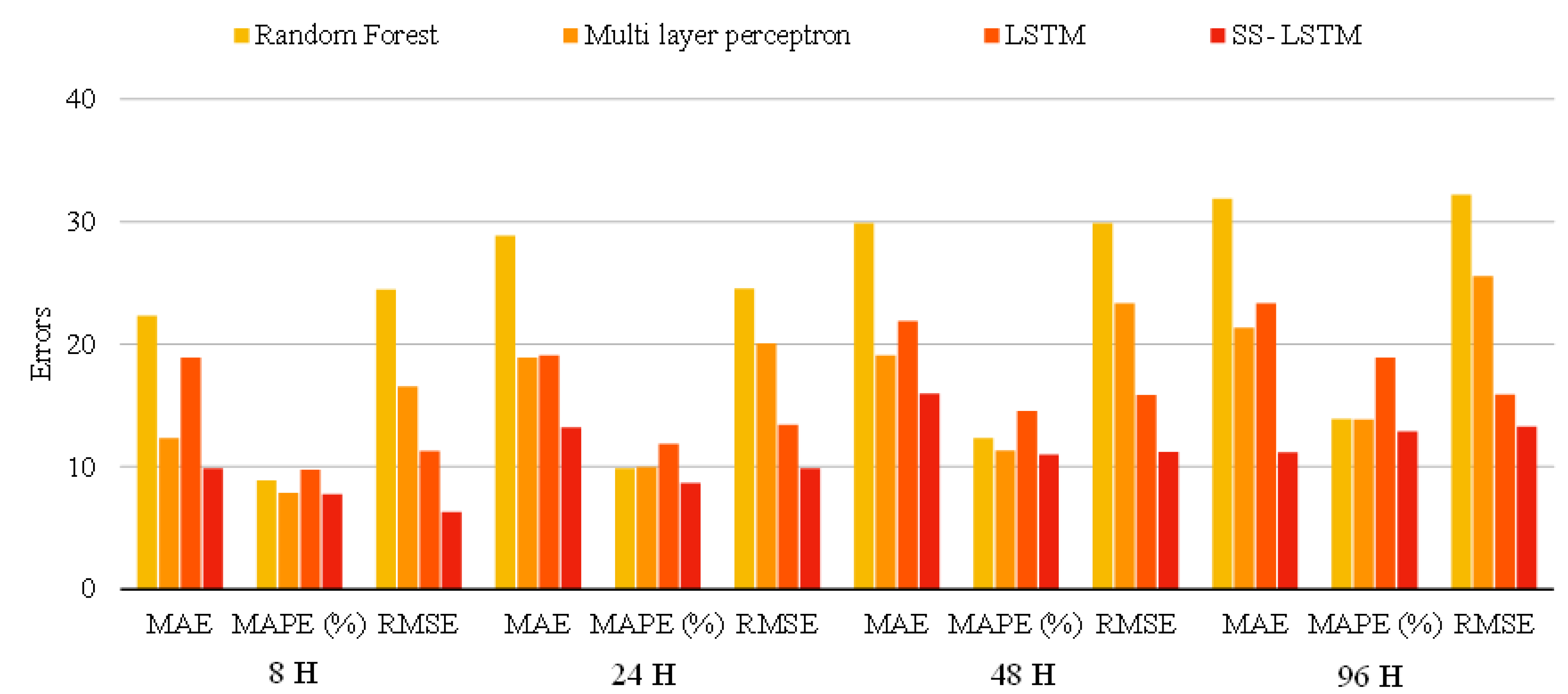
After predicting the quantity of PM2.5 and PM10 for next the 8 h, 24 h, 48 h, and 96 h and evaluating them using a variety of assessment techniques, such as MAE, RMSE, and MAPE. Random forest, multi-layer perceptron (MLP), long short-term memory models (LSTM), and seminal stacked long short-term memory (SS-LSTM) models are all analyzed and identified on the basis of their prediction accuracy of PM2.5 and PM10 concentrations. Additionally, all these models are evaluated according to their ability to predict. The findings indicate that the aggregated model that was developed has the potential to effectively increase the accuracy of predictions. In work that is currently ongoing to forecast the proportion of nitrogen dioxide, a bidirectional convolutional LSTM model is being employed. It has been demonstrated that the model is able to carry out more precise spatiotemporal analysis when temporal and geographical considerations are taken into account simultaneously [44]. The use of stacked LSTMs has matured into a reliable method for solving complex sequence prediction issues. It is possible to describe a stacked LSTM framework as merely an LSTM model that is made up of many LSTM layers, with the appropriate running of weights and biases. The hidden state below receives a sequence of outputs from the LSTM layer above, rather than yielding a single value. More specifically, one output is created for each time step of the input, as compared to one output time step in the whole set of input time steps.

Figure 2 shows the proposed seminal stacked LSTM model in which the output of one LSTM layer is fed into the input of the next LSTM layer. The series of inputs feed into the first layer of the LSTM, where meteorological parameters such as wind direction, wind speed, and temperature are fed in, while the second LSTM layer contains the pollutants information from the local station in a 20-kilometer radius, and the third LSTM consists of correlations between the other pollutants regarding PM2.5 and PM10 levels.

2.2.2. LSTM Stacked Layer 1: Meteorological Parameters

The contaminants that exist in the atmosphere are significantly impacted by a variety of meteorological phenomena. Temperature and sun radiation both have an influence on the quantity of space heating that people will require, which in turn has an effect on the amount of pollution that is emitted. Sunlight is essential for the photochemical production of oxidants, which is a necessary step in the formation of smog. The speed, turbulence, and stability of the wind all have an effect on the transport, dilution, and dissemination of pollutants. A scavenging effect is caused by the rainfall, in that it washes out (also known as “rainout”) those particles that were in the atmosphere. Lastly, humidity is a common and significant component that plays a role in determining the impact that the concentrations of pollutants have on the health of people, as well as the property and vegetation around them.

Delhi was selected for experimentation on the effect of three major meteorological parameters: temperature, wind direction, and wind speed. The SS-LSTM layer is capable of tuning the hidden state according to the factors that influence much of the pollution in other locations nearer the seashore, e.g., the Chennai wind speed triggers the pollution factor. In Delhi, the temperature is the main pollutant accumulation factor. Layer 1 of the sequenced LSTM feeds the information from the metrological parameters into the LSTM unit.

2.2.3. LSTM Stacked Layer 2: Pollution from the Local Monitoring Station

Transport, diffusion, and deposition are the three processes that are important in the formation of this particulate matter in the atmosphere. The movement that is brought about by wind flow is referred to as transport. Dispersion is caused by local turbulence, which can be defined as motions that last for a shorter amount of time than the amount of time that is needed to average out the transportation. The declining trend of pollutants in the atmosphere, which is caused by deposition processes, such as precipitation, filtering, scavenging, and sedimentation, ultimately results in the removal of the pollutants from the atmosphere and onto the surface of the earth. Every local monitoring station is mapped using data from 5 local monitoring stations, chosen to identify the maximum possible air transportation capacity in that particular locality. The overall radius covered includes 20 km to the center of Delhi. If the everyday average rises for more than 27 days, hyperparameter tuning will occur to add this information to the data from the local stations.

India is a densely populated country; air quality is monitored by 520 stations and is accumulated as per the density of the population in the metropolitan cities. Near Delhi, many stations are in position since Delhi is among the worst polluted cities in the world.

2.2.4. LSTM Stacked Layer 3: Correlation Estimation for PMs with Contributing Pollutants

The term “particulate matter” refers to both the solid particles and liquid droplets that are suspended in the air and are of a size that allows them to be breathed in. Sea salt, dust (airborne soil particles), and pollen grains are examples of natural sources of particulate matter (PM); however, it also comprises material from volcanic ash and particles generated from naturally occurring gaseous antecedents (e.g., sulfates).

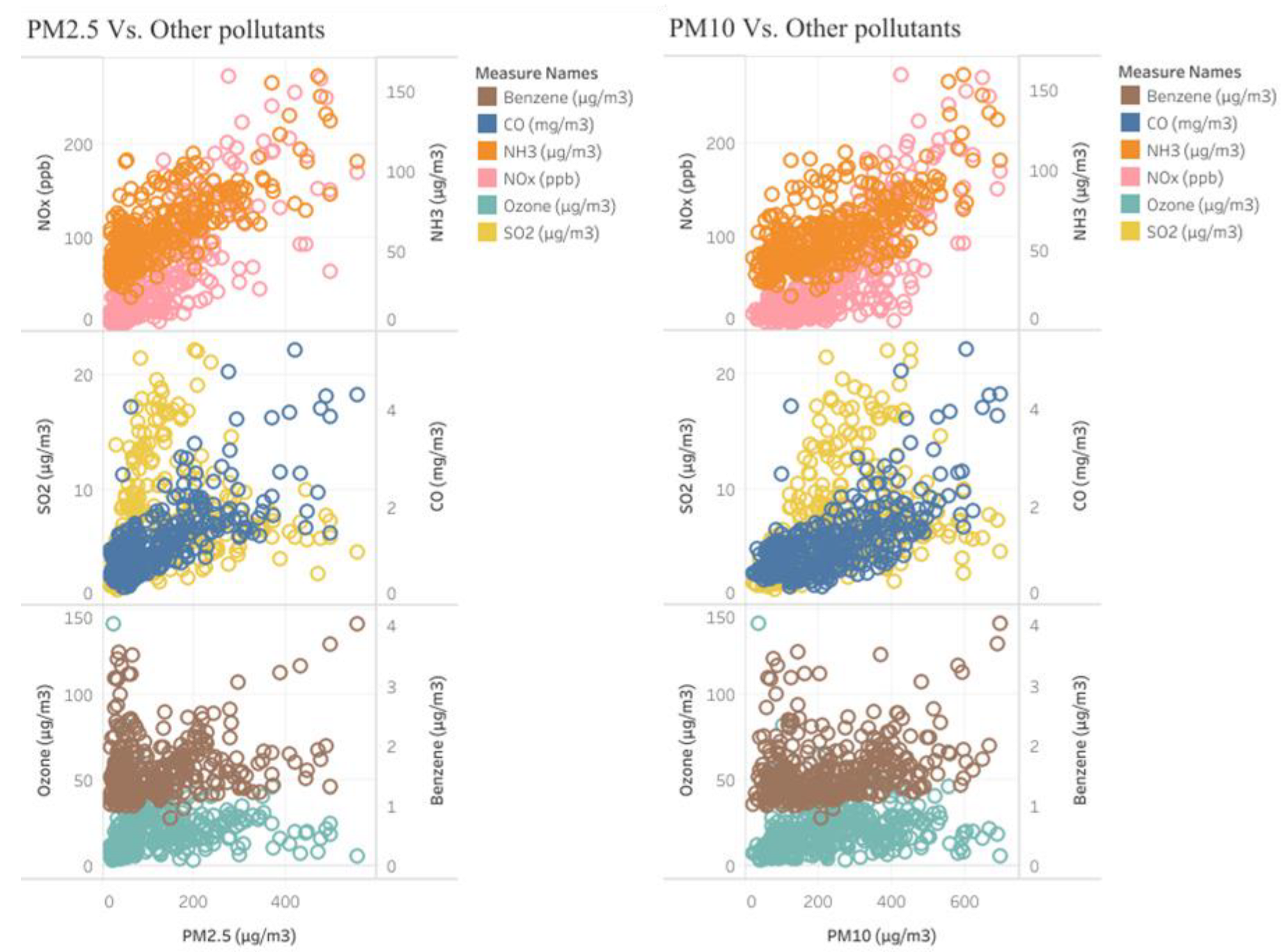
A pollution concentration of PM2.5 or PM10 varies with respect to the other major contributing pollutants. PM2.5 is one of the naturally available components in the atmosphere. Eventually, other emissions that are the predominant source of pollutants in that particular locality contribute to PMs, to a certain extent. This contribution needs to be analyzed, to ensure that the contributing pollutant still has a major impact on particulate matter. There might be primary sources of PM that already exist in the atmosphere; other pollutants that contribute toward PM values are secondary sources such as gasses from power plants, coal fires, etc. An account is needed of the relevant emissions to achieve a correlation analysis of the pollutants contributing to the PM burden. A canonical correlation of these particles gives an idea of the predominant pollutants contributing to the PM value; this is fed into the LSTM model as the input source. This refines the prediction model to improve the exact forecasting of PM2.5 and PM10. The correlation of PM2.5 and PM10 is analyzed with respect to the other predominant pollutants, as shown in Figure 3. Moreover, the behavior of other pollutants with the PM2.5 & PM10 values. The six major pollutants are shown, with the PMs and the intensity of the ranges in which they occur, for the year 2020 at the site in Delhi.

2.3. Working with the SS-LSTM Model

To build the model in an effective manner, Delhi was chosen, as the city in India suffering from the most severe PM pollution in the country. The LSTM is a special kind of RNN that is constructed from LSTM cells. An LSTM cell has the ability to control the amount of information that is saved out of its current state, as well as the amount of information that is used from past states to analyze the current state. This is made possible by internal gates that decide what information should be stored permanently and what should be forgotten before it is passed on to the next stage. Because of this property, an LSTM is able to acquire the ability to learn about long-term dependencies.

An SS-LSTM memory cell is essentially an LSTM cell that has an additional LSTM memory cell nested inside it. This internal storage cell cannot restrict the external storage cell’s ability to independently read and write the long-term information that is important to it. The general robustness of the basic LSTM perceptron is improved by this structure, which makes it possible to memorize and process information relating to a longer period of history. When it comes to LSTM, the output gate adheres to the idea that knowledge that is not pertinent to the present time point is still worthwhile to remember. According to the reasoning presented earlier, SS-LSTM is more advantageous than other methods in the forecasting of time series data that are prone to unpredictable shifts [20]. The input sequence i_n, h_t−1 indicates the output state of the hidden layer at time t−1, while W is the weight matrix of each LSTM unit. The structure of an LSTM memory cell is as follows:

i_n = Sig (W_i × [h_t−1, x_t] + v_i)

(1)

F_n = Sig (W _f × [h_t−1, x_t] + v_f)

(2)

O_t = Sig (W_o × [C_t h_t−1,x_t] +v_o)

(3)

C_t = f_t × C_t−1 + i_t × tanh(W_i × [h_t−1,x_t])

(4)

h_t = O_t × tanh(C_t).

(5)

The stacked LSTM network is made up of LSTM units and, as a result, it builds a network model with numerous hidden layers. Additionally, it continuously eliminates redundant input through the use of forget gates, in order to achieve a greater level of accuracy. As a result, the LSTM has superior performance when it comes to predicting time series. Equation (3) yields the output of weighing each neuron’s connection to another neuron inside the next input layer, and so on.

The seminal stacking of LSTM connects with a dense layer that accumulates the information in the previous three layers. To expand the number of possible storage places, it is suggested to use many LSTM models in the initial layer, rather than a single one. With this many sites, it makes sense to generate five LSTM models. The data connecting at position k to various gates in the relevant LSTM model at the first stacked layer are represented by the entire weight matrix Wxj,ki for j ∈ {i, fn, o}. Similarly, k represents the input weights, biases, gate values, cells, and instances of hidden states.

To make it easier to discuss the metrological factors for the LSTM component associated with location k for k 1,2, c, we utilize the column arrays W [l] lstm,k and R [l] lstm,k, which contain all the elements in W [l] xi,k, W [l] o,k, W [l] fn,k. Next, the input from the first layer’s concealed states is merged with information from the other locations to generate the combined output of the second layer. The terms W [l] lstm and B [l] lstm are defined in the same way, as is with the second LSTM layer. When there are two layers, and in the case of the stacked LSTM model, it is shown that the first layer’s hidden states are fed into the second layer. For the second LSTM layer, we use the same concept of w [l] lstm and b [l] lstm, but we feed in the meteorological parameters from the nearby monitoring station to account for the larger effect of pollution. However, in the location-aware stacked LSTM, each location has its own LSTM model, and the intake of the second LSTM layer is specified by a mixture of the hidden layers of the LSTM models in the first layer. Keep in mind that if there are more than two layers, the hidden state merger may occur after either the first or the second LSTM layer (the correlation knowledge of the other contaminants toward the PMs is supplied to a stacked 3-layer LSTM model) and that a thick layer is employed well after the third LSTM layer in both traditional stacked LSTMs with spatiotemporal stacking. Finally, the forecast may be made using the equations in

Table 1. LSTM Stacking with three different layers and its equations with the dense layer.

	SS-LSTM Layer 1 xt = [xt,1, xt,2, xt,3, … xt,c]	SS-LSTM Layer 2 ht [1]	SS-LSTM Layer 3 ht [2]
Equations	in [1] = Sig(Wi [1] × [ht−1 [1], xt [1]] + vi [1])	in [2] = Sig(Wi [2] × [h t−1 [2], xt [2]] + vi [2])	in [3] = Sig(Wi [3] × [ht−1 [3], xt [3]] + vi [3])
	Fn [1] = Sig (W f [1] × [ht−1 [1], xt [1]] + vf [1])	Fn [2] = Sig (W f [2] × [ht−1 [2], xt [2]] + vf [2])	Fn [3] = Sig (W f [3] × [ht−1 [3], xt [3]] + vf [3])
	Ct [1] = ft [1] × Ct−1 [1] + it [1] × tanh(Wi [1] × [ht−1 [1], xt [1]]	Ct [2] = ft [2] × Ct−1 [2] + it [2] × tanh(Wi [2] × [ht−1 [2], xt [2]]	Ct [3] = ft [3] × Ct−1 [3] + it [3] × tanh(Wi [3] × [ht−1 [3], xt [3]]
	Ot [1] = Sig (Wo [1] × [Ct [1], ht−1 [1], xt [1]] +vo [1])	Ot [2] = Sig (Wo [2] × [Ct [2], ht−1 [2], xt[2]] +vo [2])	Ot [3] = Sig (Wo [3] × [Ct [3], ht−1 [3], xt [3]] +vo [3])
	ht [1] = fn (ht−1 [1], Ct−1 [1], xt; WR [1] LSTM}	ht [2] = Ot [2] × tanh(Ct [2])	ht [3] = Ot [3] × tanh(Ct [3])
	Ct [1] = ft [1] × {Ct−1 [1], ht−1 [1], xt; WR [1] LSTM}	Ct [2] = ft [2] × {Ct−1 [2], ht−1 [2], xt [2]; WR [2] LSTM}	Ct [3] = ft [3] × {Ct−1 [3], ht−1 [3], xt [3]; WR [3] LSTM}
	ht [1] = fn(ht−1 [1], Ct−1 [1], xt; WR [1] LSTM}	ht[2] = fn(ht−1 [2], Ct−1 [2], xt [1]; WR [2] LSTM}	ht [3] = fn(ht−1 [3], Ct−1 [3], xt [2]; WR [3] LSTM}
Dense Layer	W[1] lstm, k [1] lstm—wight and residual vectors	W [2] lstm, k [2] lstm—wight and residual vectors	W [3] lstm, k [3] lstm—wight and residual vectors
	Final Prediction T + i = W [1] dense h [3] t + R [3] dense; i is the number of future time targets. W [1] dense Weight of the initial component.

.

The bias and weights terms within the dense layer are Wdense and Rdense, and q is the number of days ahead to be forecast. T is the length of the input sequence. Our studies use a nonlinear transfer function during network training and take advantage of early stopping regularization to prevent overfitting.

The suggested location-aware stacked LSTM approach benefits from fewer parameters than the stacked LSTM, among other advantages. If we suppose that the total number of neurons present in the first and second layers is the same, for example, if the number of neurons in a layered LSTM model in the initial layer is n1, then, in a stacked LSTM, every LSTM model in the first layer has n1c neurons, where c is the count of locations. Each block in the seminal stacked LSTM is associated with a specific location, just as they would be in a traditional stacked LSTM if the whole-weight matrices were diagonal. Thus, the suggested strategy requires less optimization of fewer parameters. For this reason, the location-aware stacked LSTM is preferable whenever the quantity of samples included in the training set is limited. Conversely, in models based on a stacked LSTM, the next LSTM layer combines the hidden layer from the first layer with information on the relationship between the locations.

2.4. Experimentation

2.4.1. Dataset

Data for this research study is collected from CPCB. This dataset contains 16,425 records, all of which have several characteristics at each station. The time frame for the recording runs from 1 January 2016, all the way through December 2020. The components that make up the data are as follows: the date, the concentration of PM2.5 and PM10, nitrogen dioxide NO₂, sulfur dioxide SO₂, carbon monoxide CO, ozone O₃, the temperature, wind direction, and wind speed. On the other hand, the air quality and atmospheric parameter tracking equipment will, on occasion, malfunction, which will result in a loss of data-gathering capacity. The causes for this are beyond anyone’s ability to manage. The presence of such missing numbers will have an effect in some way on the process of data mining. The missing values must be addressed in order to make the quality of the data up to a level where we can feed the data into the stacked LSTM model. The k-nearest-neighbor method is used to impute the missing values from the CPCB data. The sequence of the data that are missing continuously is taken as k in order to not alter the exact behavior of the data spread.

2.4.2. Data from Live Monitoring Station

The information for the local area is gathered from the Central Pollution Control Board. The data fields that were utilized in the compilation of the data set for the local station are presented in Table 1. Nine of the 17 dimensions included PM2.5, PM10, SO₂, O₃, NO₂, CO, wind speed, wind direction, or temperature. Three of the dimensions are methodological parameters that were recorded in that specific site. The data is sampled every 24 h; thus, the total recordings will be equal to 5 times 365, which is equal to 1825, and the overall records will be equal to 1825 × 9. Firstly, the data of these meteorological parameters are fed into the LSTM hierarchical layers, and the proposed SS-LSTM identifies the meteorological influence toward particulate matter in that particular locality. Secondly, it checks the influence of the pollutants on the PM, with respect to the neighboring stations. Third and finally, the correlation coefficient tells the maximum contributing pollutant towards the PM. This information helps in tuning the forecasting mechanism with respect to the past and present values of PM2.5 and PM10.

Constant weighting, linear weighting, and random rank weighting are the three different types of full predictive qualities that may be utilized in this model’s predictive capability. When aggregated using a uniform method, the ratings of each prediction feature are kept the same. However, the causes of air pollution should be different at various times or in different station locations, depending on where the sample is taken. The idea of linear aggregation serves as the foundation for this investigation. Three distinct models each create their own unique set of characteristics, and each of those characteristics is assigned a unique weight [40]. The aggregation learning algorithm generates three prediction features for the many different sorts of stations. The data are produced using functional predictions made by the densely integrated neural network layer. Instantaneous data training and weight changes via reverse propagation are incorporated after each batch in the system [45]. The best possible outcomes can be accomplished in the end. The SS-LSTM model’s methodology for predicting PM2.5 and PM10 is broken down into the following subsections.

The prediction is learned by our model by means of a neural network. LSTM is a fodder neural network with the ability to simulate the sequential data referred to as RNN. It does so by distributing the weight of each component in the sequence throughout the span of time. RNN may be implemented in a wide variety of ways. In the most fundamental version of RNN, the phase is a Fourier transform of the previous hidden vector, h, and the input vector, x, accompanied by an activation function addressing non-linearity. This linear transformation is accompanied by an activation function. The weight matrix is denoted by W, the bias vector is denoted by b, and the activation function is denoted by tan h. The traditional version of RNN takes the shape of a series of neural network modules that may be repeated, and its design is quite simple. RNN is capable of learning long-term reliance, at least in theory. As a general proposition, however, it is plagued by the vanishing gradient problem, as well as the expanding gradient problem, as a consequence of its long-term reliance. As a result of this reliance, RNN is rendered less effective and more difficult to train [46]. By employing the idea of memories, the gate design, and the constant error carousel, the LSTM network is able to mitigate, to some extent, the long-term reliance problem. Because there are dependencies upon immediate prior entries, as in the example using the sequential diabetes patient data, LSTM is better suited to model PM2.5 and PM10. This is because LSTM can represent and relate dependencies.

2.4.3. Working of SS-LSTM with Respect to the Input Sequence

Because of the relation toward the dependencies, it is evident that the SS-LSTM-based model is superior to the other model designs in terms of its ability to produce accurate predictions. The SS-LSTM network comprises 142 hidden-element variables. At stage t, each cell has a forget gate denoted by f_t, an input gate denoted by i_t, a control gate denoted by C_t, an output gate denoted by O_t, and also an internal cell recall denoted by C’_t. The first gate is called the forget gate ft, and its purpose is to decide which pieces of information may be brought into the cell out of the output of the LSTM cell that came before i_t. The input gate determines the degree to which the fresh memory should have an effect on the previously stored information. The control gate C_t produces fresh memory and uses the information provided by C_t−1, and C_t, to update the cell state. The symbol in this context denotes element-wise multiplication, along with the memory needing to be captured. The modulation of the output in order to achieve h_t−1, is the responsibility of the output gate. The associated weight matrix is denoted by Ws in the aforementioned equations. The sigmoid activation function and the hyperbolic tangent activation function are denoted by the logit function and tan h, respectively.

After the hidden state of SS-LSTM comes the dropout layer, which is added to avoid the overfitting of the model, but further normalization is used to avoid overfitting. Dropout is implemented with the goal of minimizing model overfitting, also enhancing its ability to generalize [47]. A vector called hi is output by the final layer of the LSTM; this vector is then fed into the fully linked multi-layer network as its input. This network has a total of three layers, with one output layer and two hidden layers included in its construction. These three densely layered hierarchical structures each have 18 neurons, 142 neurons, and 512 neurons, respectively, which are equipped with an activation function. For the first two dense layers, we will use an activation function known as the rectified linear unit (ReLU), while for the output layer, we will use an activation function known as the exponential function. In this case, layer 1 denotes the mean, while 2 refers to the variance. With these data, we are able to complete an evaluation of the model’s level of confidence. A multi-dimensional series of preprocessed data serves as the model’s input. The outcome of the algorithm is a forecast regarding the level of PM2.5 and PM10 within a given time horizon for the prediction. We conduct experiments with an 8-hour, 24-hour, 48-hour, and 96-hour timeframe for our predictions.

If the value is getting closer to 0, it indicates that the status of the neuron is going to be fully forgotten, but if it is getting closer to 1, this indicates that the condition of the neuron is going to be completely remembered. The procedure allows us to forget whatever information has been forgotten about the cell state. Then, we multiply the data that needs to be memorized by the output of the input gate to obtain the information that needs to be memorized. Finally, we choose the array of data that needs to be memorized by using the output of the input gate. After this, we utilize matrix addition to add up to identify the receiving cell that has already emerged from the forget gate. This allows us to memorize the information that has already been memorized and to produce the function of the cell at that particular time.

In order to prevent our LSTM layers from being too fitted, we have inserted two dropout layers between them. During each stage of the learning process, we render fifty percent of the cells ineffective to avoid the neural network’s utilizing more complex approaches. These methods result in a nearly flawless conversion to the training set, but they do not adapt well to unknown data. The nerve cells are going to be converted into solid lines, and these lines will contribute weights to the entire neural network and to the updated weights. Because of this, the dropout layer will be able to render the neurons unreliable in order to prevent overfitting. In total, 18 neurons are capable of making the connections between the 142 neurons to the second LSTM protocol stack and to all 512 neurons of the comprehensive third layer. This allows the fully connected layer to generate an auspicious weight with the activation function of its next fusion layer, which in turn leads to a series of outputs that are desired for the prediction horizon. The combination of the next three sub-neural networks is achieved using a fusion layer. This layer combines the feature data that are produced by the sub-stacked LSTM networks with the feature data that are generated by the fully connected layer that comes after it. This technique gathers all the anticipated characteristics and output for the subsequent layer, and then assigns a different weight to each of the predicted features.

3. Results

To make the model fit, we will integrate the last complete layer with the input of the fusion layer’s prediction features. Backpropagation will be used in the final layer to assign varying weights toward its hidden units, so as to calculate the PM2.5 and PM10 values that are projected to be present in the next 8 h and 24 h. In order to obtain the final PM2.5 and PM10 ranges that have been predicted by the neural network, the data will be combined with the final result of the network. The final layer might indicate the correlation of the neighboring station data for each anticipated feature by assigning various weights to the forecasted characteristics. When a station is placed in a city such as Chennai, in the coastal area, it is necessary to take into consideration the fact that PM2.5 might have a larger value when external pollution generators are blown off-course, either by the monsoon, when the wind current is heavy, or when climate conditions are unfavorable. Both the rate of wind speed and the orientation of the wind are critical factors that influence the dispersal of air pollution [48,49].

Alterations in both the wind’s velocity and its direction are typical of each new season. As a result, the initial phase of the monsoon will play a significant role in the process of forecasting air pollution, particularly in the western parts of the country, which experience their respective initial monsoon bursts only once every year. These are going to be the first regions on which the monsoon will have an effect. In the course of this investigation, later, the dry wind accumulated and reached Delhi, bringing high humidity. This allowed us to carry out a dispersed and accurate analysis of PM2.5 and PM10, which was necessary, given that these wind directions are more likely to be affected by the increased wind direction and wind speed in this area than in any other locations. As a result, the stations in the north give less consideration to the projected features of other pollutants in the south, while the locations in the south give more consideration to the anticipated possibility of other emissions [50].

The stacked LSTM has 142 memory units and return sequences; it employs the meteorological characteristics of the nearby station, the influence on PM2.5 and PM10, and the correlation of key pollutants with PM2.5 and PM10 as its three input layers and three sub-network layers. In conclusion, the final layer is a completely integrated fusion layer that optimizes the integrated input layer containing all three components, in order to generate a unified prediction range of desirable values.

Evaluation of the Results

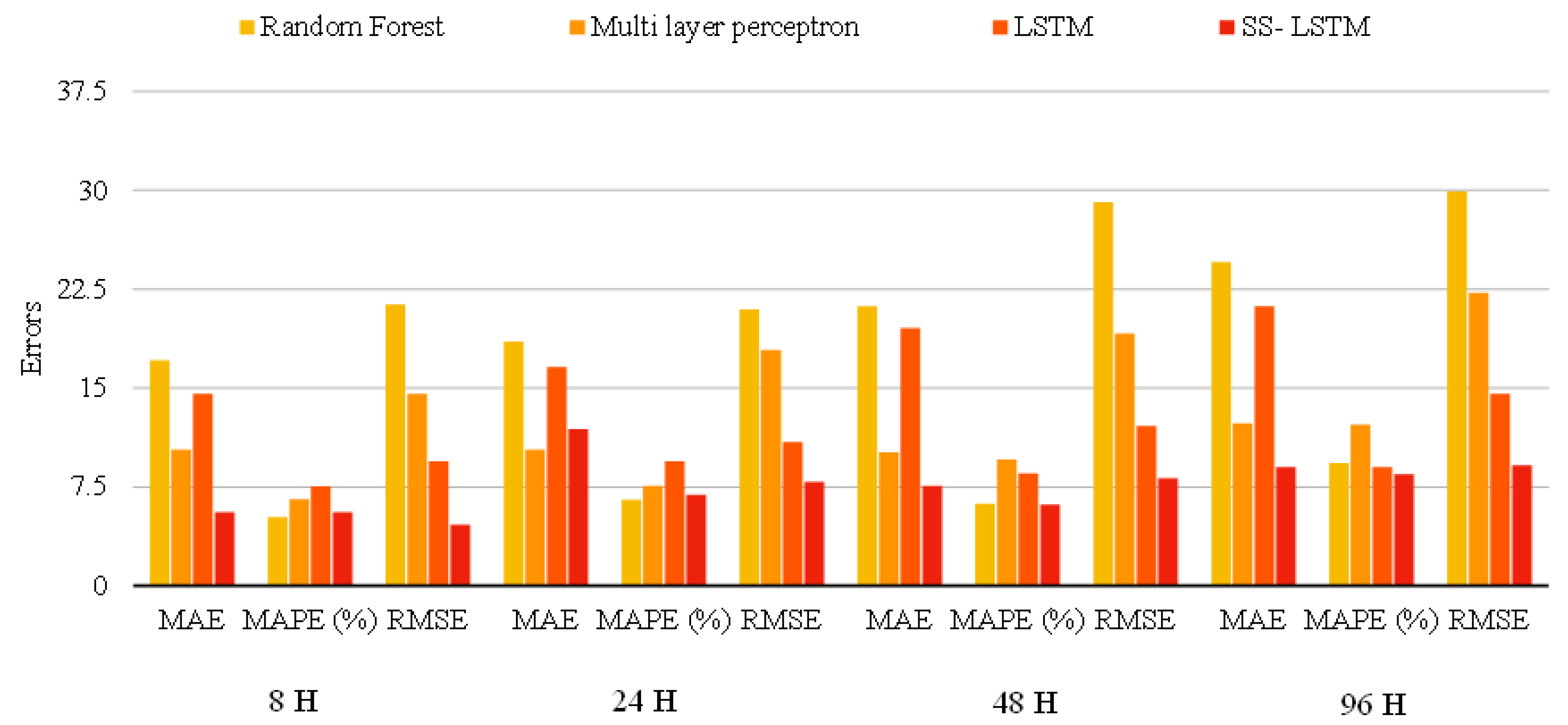
The mean absolute error (MAE), mean absolute percentage error (MAPE), and root mean square error (RMSE) are three statistical approaches that may be used to determine the amount of deviation that exists between the actual and the projected values (MAPE). In this proposed research work, a comparison between the error values of RMSE is evaluated, as shown in Equation (6), with MAE and MAPE for the models of random forest, multi-layer perceptron, LSTM, and SS-LSTM. The root mean square error, or RMSE, is a measure of the disparity between the projected value and the true value. The primary application for it is in the computation of the values at various time intervals. When the score is greater, the forecast is off-kilter to a greater degree. The MAE refers to the overall absolute distance that exists between the two values. There is really no negative or positive phase cancellation, and the MAE is absolute when related to the mean error. This is because the dispersion causes the mistake. Therefore, the standard deviation of the error rate is the same.

MAPE is a statistical metric that may be used to evaluate how accurate a certain forecasting method is. This “accuracy” is expressed as a percentage, and the mean percentage percent error may be computed for each period by first subtracting the real values from the calculated ones, then dividing the resulting number by the calculated ones. However, the absolute distance in the inaccuracy to be found in the forecast will increase in proportion to the concentration of the variable being studied. As a result, we have great hopes that the MAPE will be able to create forecasts that have the highest accuracy among several regional models.

RMSE = √[Σ(Pi − Oi)2/n]

(6)

MAE = 1/n Σ {(Pi − Oi)/n}

(7)

The SS-LSTM network’s unique inner set of connections is responsible for the majority of the outperformance, while training time is kept to a minimum. While stacking several LSTM layers improves the prediction accuracy in SS-LSTM neural networks, the stacking design doubles the hyperparameters in the optimization procedure. The SS-LSTM training process usually takes substantially longer to compute than the LSTM training procedure. As a result of our findings, the SS-LSTM model is better suited for air-quality index time-series forecasting than other LSTM extensions. The suggested and compared methods utilize a data modeling strategy, employing a memory unit that is fed with historic inferences that are used to stabilize the actual AQI variable data. As can be seen in Table 1, when multiple LSTM models are combined, the prediction performance improves significantly, and the prediction latency decreases. This result demonstrates the need to use stacked-LSTM approaches to stabilize the original data. As the prediction horizon grows longer, it is clear that the level of inaccuracy will grow as well. Figure 4 and Figure 5 depicts a comparison of the errors with respect to the time target we used to forecast.

The model shows the greater impact in prediction accuracy where prediction horizons have different prediction accuracy performance values. The larger horizons will demonstrate better forecasting than the smaller time horizons. The seminal stacked LSTM offered various insights with the contributions towards the PM. The correlation analysis information helps to build the model more stable, while the correlated pollutants derived from the historical data make the model stronger, even if the prediction horizon window is large. Once the stacking of the LSTM model is achieved, the activation parameters help to decide the forecasting model. Forecasting models rely purely on the information in the memory gates of each LSTM, which is a perfect choice to ensure the fitness of the forecasting model.

Table 2. Data collected from the CPCB and its unit of measurement.

Parameter	Samples	Unit of Measurement
PM2.5	12 h	μg/m3
PM10	12 h	μg/m3
CO	12 h	μg/m3
NO2	12 h	μg/m3
SO2	12 h	μg/m3
O3	12 h	μg/m3
Temperature	24 h	°C
Wind speed	24 h	m/s
Wind direction	24 h	degrees

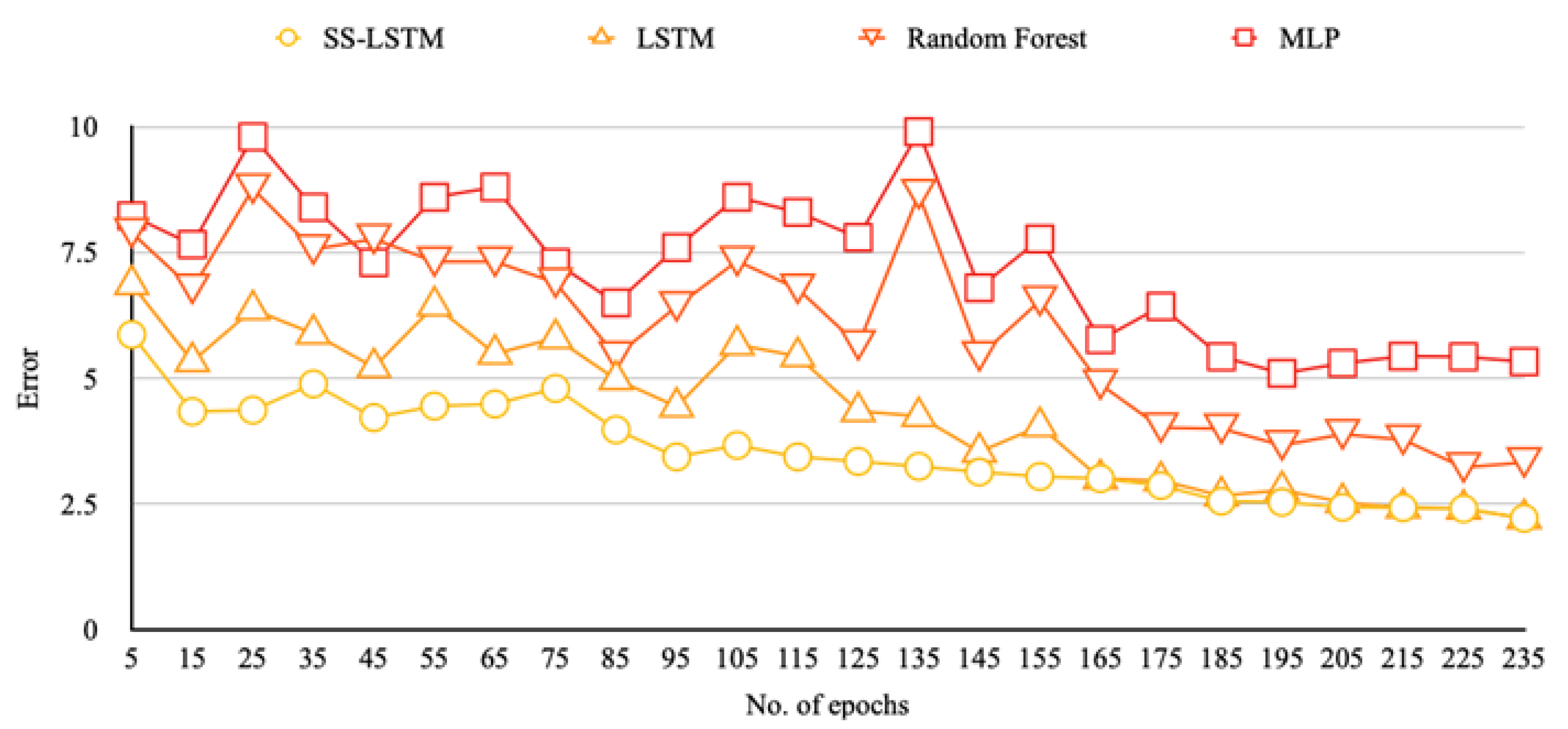
. Shows the measurement unit and the collected instants of the each pollutants. Figure 6. Depicts the reduction in error with respect to the no. of epochs we train the model.

4. Discussion

Pollution is a major environmental phenomenon that has a direct impact on human life. Pollution is dependent on other environmental parameters, such as wind speed, wind direction, temperature, and relative humidity. This is the predominant factor with respect to any location to be assessed when analyzing the particulate matter values. These meteorological influences are taken into account in the layer 1 LSTM units. The pollution may disperse and may act as a source for some of the other neighboring areas. The dispersion of airborne particles will create new pollution levels in the neighboring stations. The sudden change in pollution values (peaks) should be considered when accounting for the pollution scattered through air dispersion, as recorded by the local pollution monitoring centers. This information on the neighboring pollution variations can be given to the second-level stacked LSTM units. The final layer of LSTM units consists of information from the correlation analysis of the other pollutants regarding the particulate matter.

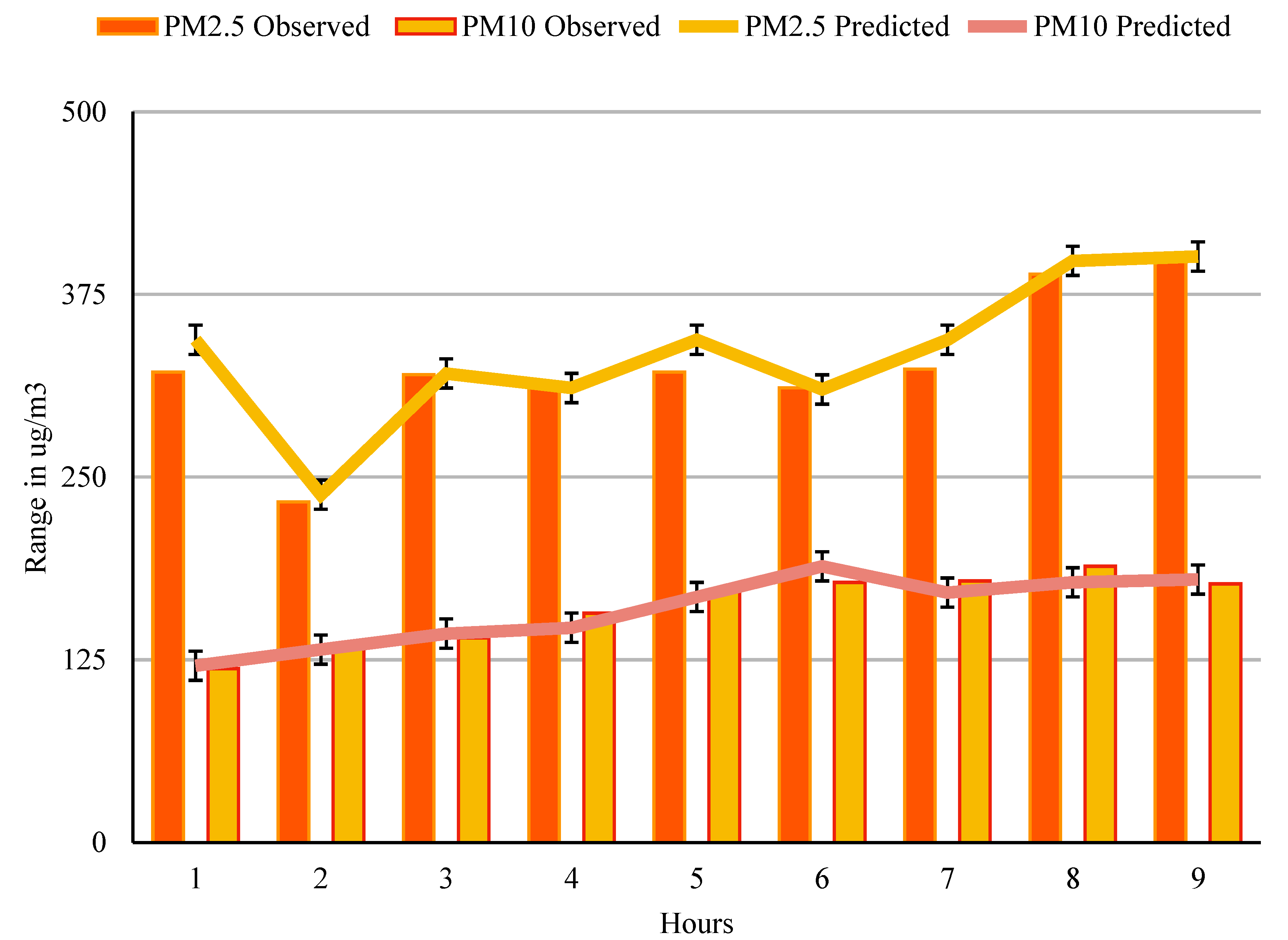
The trends and the improvements in forecasting are evident when analyzing the proposed method. It is clear the error deviations over the prediction are both positive and negative. Figure 6 shows the variations in terms of the observed value and the predicted value. The observed values are drawn from the relative data collected from the central pollution control board. These data are compared with the predicted values using the seminal stacked approach. The deviation of error is on both positive and negative ends but it is not more than ± 15, the advantage offered by the proposed method to predict the real-time values, which are very close to the observed values. The Delhi prediction for the date 1 October 2022, using the proposed method, gives the increasing values for the particulate matter in that locality; it is necessary to predict accurate values to take appropriate action. As seen in databases from all over the globe, Delhi is one of the most polluted cities with respect to particulate matter.

The number-missing prediction builds the certainty of the model. If the model is only certain enough if it reaches the uncertainty quotient of less than 10%. Using the aleatoric uncertainty estimation method, it proves its randomness in nature, and the uncertainty level is less than 10%. Uncertainty in predictions is reflected in the range of possible outcomes that may be attributed to a wide variety of possible inputs. A probability density function for model predictions is formed as an uncertainty about the correct input values is propagated throughout the model. The reliability of the experimental or computational results is determined in large part by the uncertainty quantification (UQ) process. Figure 7. Shows the variation of observed and predicted values using SS-LSTM method.

The biracial approach of these LSTM models gives the appropriate weighting to the units that needed to be considered in order to build the forecasting model. The proposed model covers the impact of full parameters regarding particulate matter. The environmental factors affecting the pollutants is collected from local neighboring monitoring station finally merge with the same station’s major pollutants. This helps in identifying the contributing to particulate matters.

5. Conclusions

This article proposes a unique SS-LSTM learning system for predicting particulate matter pollution concentrations. The PM2.5 and PM10 training and forecasting processes are computed in relation to their source. The data were processed in parallel and aided by federated learning. According to the findings of the experiments, the suggested method was effective in tracing the actual PM2.5 and PM10 levels extremely closely, with MAE, RMSE, and MAPE values that were all lower than those predicted by the existing methods. By providing timely atmospheric information to the government, reliable air pollution forecasts can assist in environmental managerial decisions and are vital for human health. A real-world data set collected by meteorological stations in and around Delhi, India, was used in the experimental phase. The suggested method outperformed most of the conventional systems compared in SS-LSTM-based PM forecasting, according to the results and comparisons. In comparison to the previous techniques, the suggested model could execute predictions with significantly less error and nearly no lag in trend. The findings demonstrated that the suggested deep learning framework is well suited to multivariate AQI forecasting. By dividing the original information into high-frequency and low-frequency parts and learning them separately in a multi-feature module, the suggested method distinguished the features and trends. During the training procedure, the sub-LSTMs predictions were merged and optimized to generate the forecast of each variable with the best weights and bias. The multi-layered structure provided the capacity to learn numerous meteorological variables concurrently. After analyzing the input from the other local pollution monitoring centers, the multi-correlation conducted and optimized the predictions of each variable.