The Seismo-Ionospheric Disturbances before the 9 June 2022 Maerkang Ms6.0 Earthquake Swarm

Abstract

Based on the multi-data of the global ionospheric map (GIM), ionospheric total electron content (TEC) inversed from GPS observations, the critical frequency of the F2 layer (f_OF₂) from the ionosonde, electron density (Ne), electron temperature (Te), and He⁺ and O⁺ densities detected by the China Seismo-Electromagnetic Satellite (CSES), the temporal and spatial characteristics of ionospheric multi-parameter perturbations were analyzed around the Maerkang Ms6.0 earthquake swarm on 9 June 2022. The results showed that the seismo-ionospheric disturbances were observed during 2–4 June around the epicenter under quiet solar-geomagnetic conditions. All parameters we studied were characterized by synchronous changes and negative anomalies, with a better consistency between ionospheric ground-based and satellite observations. The negative ionospheric anomalies for all parameters appeared 5–7 days before the Maerkang Ms6.0 earthquake swarm can be considered as significant signals of upcoming main shock. The seismo-ionospheric coupling mechanism may be a combination of two coupling channels: an overlapped DC electric field and an acoustic gravity wave, as described by the lithosphere–atmosphere–ionosphere coupling (LAIC). In addition, in order to make the investigations still more convincing, we completed a statistical analysis for the ionospheric anomalies of earthquakes over Ms6.0 in the study area (20°~40° N, 92°~112° E) from 1 January 2019 to 1 July 2022. The nine seismic events reveal that most strong earthquakes are preceded by obvious synchronous anomalies from ground-based and satellite ionospheric observations. The anomalous disturbances generally appear 1–15 days before the earthquakes, and the continuity and reliability of ground-based ionospheric anomaly detection are relatively high. Based on the integrated ionospheric satellite–ground observations, a cross-validation analysis can effectively improve the confidence level of anomaly identification and reduce the frequency of false anomalies.

1. Introduction

Earthquakes are among the most threatening and destructive natural disasters to human beings. However, the short-term monitoring and prediction of earthquakes remains a scientific challenge to be solved. In recent decades, pre-seismic ionospheric anomalous disturbances were commonly detected, and seismo-ionospheric effects have attracted extensive attention from geophysicists. More and more published studies have found that seismo-ionospheric disturbances such as electron and ion density depletion and/or enhancement occurred a few hours to several days before the earthquakes around the epicenter, which were probably signs of a impending main shock [1,2,3,4,5,6,7,8]. Liu et al. [1] statistically analyzed earthquakes of a magnitude over 6.0 in Taiwan during 1994–1999, and the results showed that seismo-ionospheric signatures appeared 1–6 days prior to these earthquakes in the form of the falling f_OF₂ recorded. According to the statistical analysis of ionospheric anomalies before 736 M6.0+ earthquakes during 2002–2010, Le et al. [5] illustrated that the anomalous behavior of electron density within just a few days before the earthquakes was related with the forthcoming earthquakes with high probability. Devoted to a statistical analysis of the night-time ion density variations, Parrot et al. [8] found that the intensity of ion density perturbations was larger prior to the earthquakes than random events, and that the perturbations increased with the earthquake magnitudes. With the diversification of ionospheric detection means, we also have a more comprehensive understanding of pre-seismic ionospheric anomalies and seismo-ionospheric coupling mechanisms.

In terms of ionospheric monitoring means, ground-based ionospheric detection techniques have been widely used for earthquake precursor monitoring and research. Continuous global positioning system (GPS) observations are used to invert the ionospheric total electron content (TEC), and vertical ionospheric observations are used to obtain the critical frequency of the F2 layer (f_OF₂). The results of many scholars have shown that anomalous variations of TEC and f_OF₂ often appear before the strong earthquakes around the epicenter [9,10,11,12,13,14]. For example, Liu et al. [9] detected the pre-seismic TEC anomalies of the Chi-Chi Mw7.7 earthquake that occurred in Taiwan on 20 September 1999 and found that the equatorial anomaly crest moved equatorward and its TEC value significantly decreased 1, 3, and 4 days before the earthquake around the epicenter. Similarly, Chuo et al. [11] analyzed the variations of f_OF₂, observed by the Chung-Li ionosonde station, and illustrated that the f_OF₂ decreased significantly before the three earthquakes of a magnitude over 6.0 in Taiwan. On the basis of the GPS observation data, Zhu et al. [14] analyzed the Wenchuan Ms8.0 earthquake on 12 May 2008 in China, results showed that the apparent anomalous reduction in the TEC occurred on 29 April and 6–7 May, and the anomalous crest of the TEC moved towards equator.

However, with the fast development of space exploration technology, space electromagnetic monitoring satellite has made it possible to move from ground-based to satellite detection. A lot of new results have been published on the basis of measurements from satellites, such as DEMETER, COSMIC, and Swarm [15,16,17,18,19,20]. Many scholars have also confirmed that the electron density (Ne), electron temperature (Te) and ion density (Ni) in the ionosphere will change before the strong earthquakes. For example, Parrot et al. [15] studied the ion density recorded by DEMETER satellite, and found that the number and the intensity of the ionospheric perturbations were larger in relation with the seismic activity. Similarly, by using the DEMETER satellite to study earthquakes with a magnitude over 7.0 from 2004 to 2010, Zhang et al. [16] revealed that there were increases in the number of electron bursts prior to 6 strong earthquakes. In addition, De Santis et al. [17] analysed the ionospheric disturbances of 12 strong earthquakes from 2014 to 2016 by Swarm satellites. They found that most of the earthquakes over M 6.1 showed some precursory anomalies in the ionospheric magnetic field and electron density.

Based on the experience of foreign electromagnetic satellite research, the China Seismo-Electromagnetic Satellite (CSES) was launched successfully on 2 February 2018. The rich ionospheric detection payloads help us to understand the physical nature of ionospheric anomalies more comprehensively and probe the source of pre-seismic anomalies directly [21,22,23].

There are temporal and spatial characteristics of ionospheric anomalies induced by earthquake, which provide an opportunity for us to study ionospheric precursors. Currently, integrated satellite–ground observations have become the most effective monitoring means for ionospheric anomaly detection. On the basis of this, Akhoondzadeh et al. [24] analyzed the variations of the electron and ion densities before 4 large earthquakes. The statistical results showed that positive and negative anomalies in both of DEMETER and TEC appeared 1 to 5 days before the earthquake events, which were highly regarded as seismo-ionospheric precursors. Zhang et al. [25] combined and analyzed multi-physical observational parameters recorded by CSES and GPS weeks before the Indonesia Ms6.9 earthquake occurrence on 5 August 2018. The synchronous disturbances were found in the electron density and the ULF electric field recorded onboard CSES, and sometime on the same day in GPS TEC from NASA/JPL.

Based on the complex precursor anomalies, scientists have been focusing on the seismo-ionospheric coupling mechanism [26,27,28,29,30,31,32,33,34,35]. Currently, three main models are used to explain the precursor anomalies. The first one is lithosphere–atmosphere–ionosphere multi-channel coupling model, proposed by Hayakawa [26], which contained three channels: an overlapped DC electric field, an acoustic gravity wave and an electromagnetic wave. The model delineates the coupling process of different parameters in detail, which is beneficial to the understanding of earthquake incubation process and precursor anomalies. The second one is unified lithosphere–atmosphere–ionosphere coupling model, proposed by Pulinets and Boyarchuk [29]. The model assumes that the propagation of acoustic gravity waves can be coupled to the ionosphere through the anomalous electric field, while the changes in heat sources and water vapor are also directly associated with the anomalous electric field. The third one is lithosphere—coversphere—atmosphere coupling model, proposed by Wu [34]. For explaining the formation mechanism of the thermal infrared anomalies, the model suggests that the source of the anomalies is mainly the stress-enhancing effect during the earthquake incubation process, which eventually leads to temperature changes at the surface and near the surface. In contrast, the first model provides a clearer analysis of the physical parameters for different earth spheres and is easier to simulate digitally [35]. At present, the seismo-ionospheric coupling mechanism is still in the qualitative analysis stage. Advances in different detection techniques and analysis methods are particularly critical for future research on seismo-ionospheric coupling mechanism.

In this paper, we studied the temporal and spatial ionospheric disturbances potentially related to the Maerkang Ms6.0 earthquake swarm occurred on 9 June 2022, and statistically analyzed multiple strong earthquakes of over Ms6.0 in the study area (20°~40° N, 92°~112° E) from 1 January 2019 to 1 July 2022. Section 2 describes the data and analysis methods. Section 3 shows our results and analysis. In Section 4, we summarize the characteristics of seismo-ionospheric disturbances and discuss the seismo-ionospheric coupling mechanism. Finally, the conclusions are drawn in Section 5.

2. Data and Methods

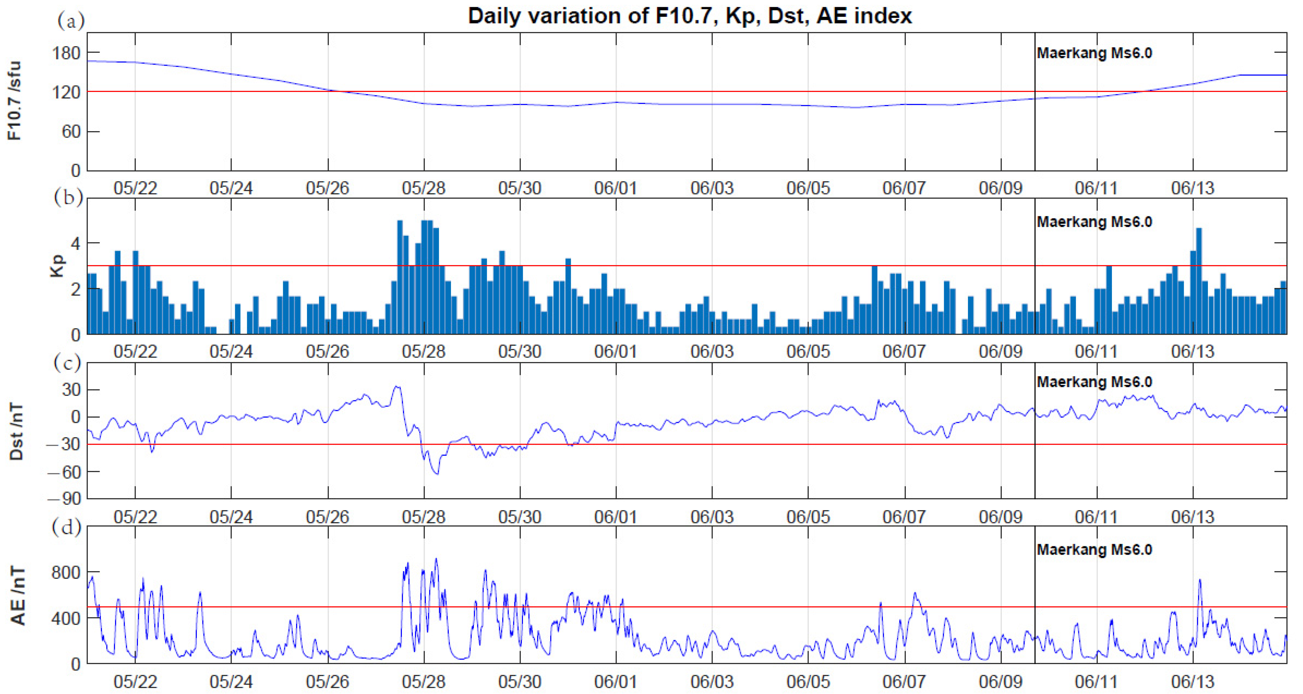
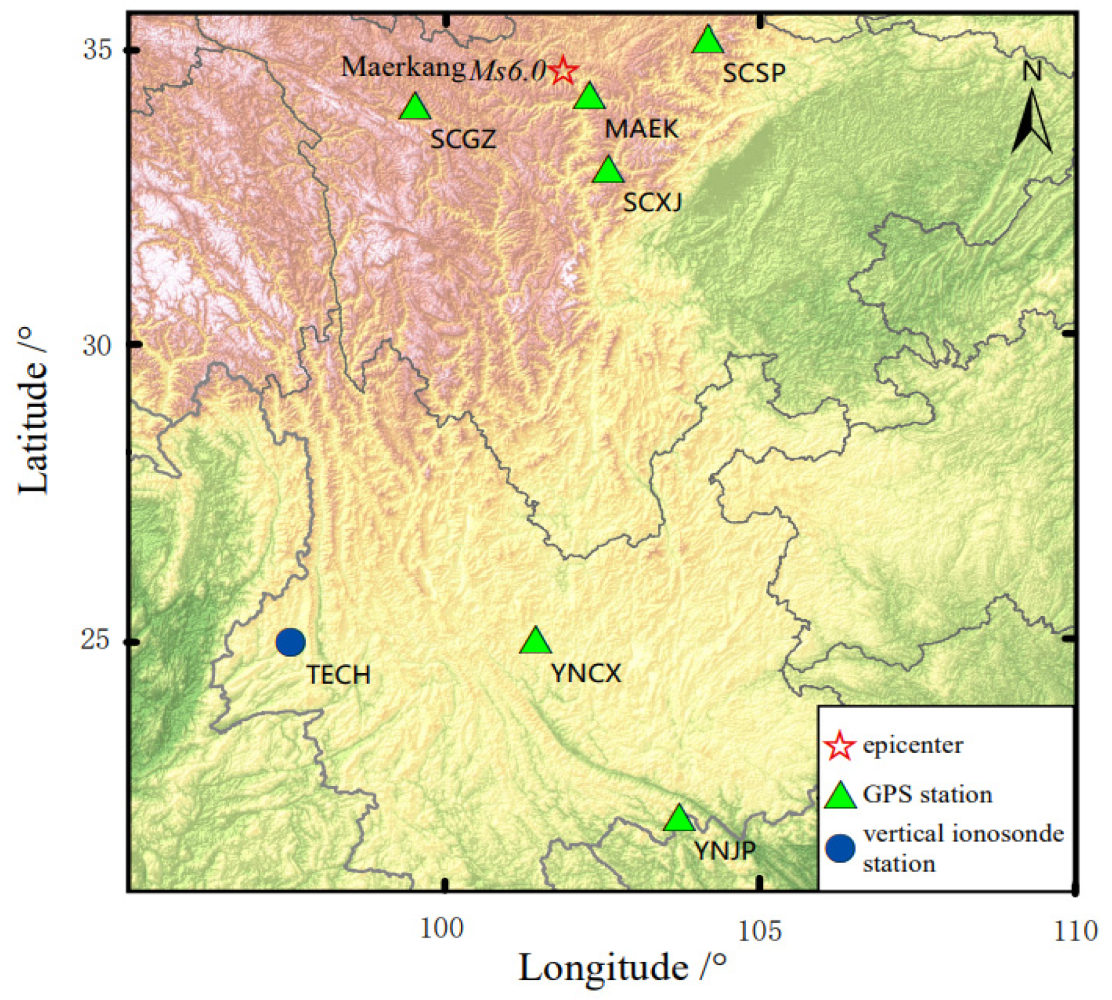
2.1. Earthquake and Solar-Geomagnetic Data

The Ms6.0 earthquake swarm occurred on 9 June 2022 in Maerkang City, Sichuan Province, China. Along with Ms5.8, the Ms6.0 and Ms5.2 earthquakes occurred successively, the epicenters are all located in Caodeng Township, approximately 53 km from Maerkang City. The detailed information of these three earthquakes is shown in

Table 1. Detailed earthquake information.

No.	EQ Date and Time (UT)	Lat./°N	Lon./°E	Ms	Depth (km)
1	9 June 2022 16:03:09	32.27	101.82	5.8	10
2	9 June 2022 17:28:34	32.25	101.82	6.0	13
3	9 June 2022 19:27:00	32.24	101.85	5.2	15

. Earthquake occurrence time is converted to Universal Time (UT).

Since both solar activity and geomagnetic perturbations cause anomalous ionospheric disturbances, we performed statistical analysis on four indices—F10.7 (http://www.sepc.ac.cn, accessed on 10 August 2022), Kp (https://www.gfz-potsdam.de, accessed on 10 August 2022), Dst (https://wdc.kugi.kyoto-u.ac.jp, accessed on 10 August 2022), and AE (http://www.sepc.ac.cn, accessed on 10 August 2022). Among them, the F10.7 index reflects the solar activity, Kp and Dst indices reflect the geomagnetic perturbations, AE index reflects the intensity of ionospheric substorm. We will only analysis the data under quiet solar-geomagnetic conditions (F10.7 < 120SFU; Kp < 3; Dst > −30 nT; |AE| < 500 nT) in this work. The changes of each index from 21 May to 14 June 2022 are shown in Figure 1. The results show that solar activity was strong on 21–25 May and 12–14 June, geomagnetic perturbations were strong on 27–31 May, with the Kp index reaching 5, the Dst index below −60 nT and the AE index exceeding 800 nT, accompanied by strong magnetic storms and substorms in above periods. In addition, the AE index exceeded 600 nT on 7 June, which may be accompanied by substorms. Based on the results, the anomalous ionospheric disturbances found in above time periods should first consider the disturbance factors of solar-geomagnetic activity.

2.2. Ground-Based Data

Ground-based ionospheric data have been used to detect anomalous ionospheric disturbances, mainly including the global ionospheric map (GIM), GPS TEC and f_OF₂. The GIM is generated by data from nearly 400 GPS stations distributed around the world. We selected the GIM data released by the Center for Orbit Determination in Europe (CODE, http://ftp.aiub.unibe.ch/CODE/, accessed on 10 August 2022), and extracted anomalous ionospheric disturbances with a spatial resolution of 5° longitude and 2.5° latitude. A total of 12 ionospheric TEC anomaly distribution images covering the whole world can be generated daily in a 2 h interval.

However, GIM uses fewer GPS stations in the gridding process and its temporal and spatial resolution is not high in China. In order to obtain higher accuracy and temporal resolution, GPS TEC inversion algorithm was used to generate single-site ionospheric VTEC with a sampling rate of 15 min [36]. In this work, we obtained GPS TEC time-series data from six GPS stations in Sichuan and Yunnan regions, which can better reflect the details of anomalous ionospheric variations on a small scale.

In addition, the f_OF₂ obtained from ionospheric vertical measurements has a high accuracy and can be used as a reference source to check other data in multi-parameter observations. Therefore, we selected the f_OF₂ data from the vertical ionosonde station in Sichuan–Yunnan region, and analyzed anomalous ionospheric disturbances combined with the GIM and GPS TEC.

The epicenter and station distribution are shown in Figure 2, in addition to the Maerkang GPS station at the epicenter, we selected one GPS station to the west, the east and the south of epicenter. We did not find available GPS stations on the north side of epicenter, nor suitable ionosonde stations near the epicenter. Meanwhile, the anomalous ionospheric disturbances were also detected at GPS stations in Yunnan, so we selected two of them and further verified the anomalies by the temporal variations of f_OF₂ from the Tengchong vertical ionosonde station. The 20 days before and 5 days after the earthquake were selected as the analysis period.

2.3. CSES Data

The CSES is the first satellite of the China Geophysical Field Exploration Satellite Program. Eight scientific payloads are onboard the CSES, which are used to monitor and study physical phenomena such as the electromagnetic field, plasma and high-energy particle sedimentation in global space. CSES transits in a solar synchronous orbit with an altitude of 507 km, orbits the Earth approximately 15 times a day with a revisiting period of 5 days, descending node at LT14:00 in daytime and ascending node at LT02:00 in the nighttime. Since the ionospheric variations at night are relatively less disturbed by solar activity, only nighttime data are utilized in this paper.

The Langmuir probe (LAP) and the Plasma analyzer package (PAP) (http://www.leos.ac.cn, accessed on 10 August 2022) are the space plasma in situ detection payloads, with both survey and burst operational modes [21]. CSES switches to the burst mode when passing through major global seismic zones and the Chinese region to provide higher sampling rate data. The LAP mainly detects electron density (Ne) and electron temperature (Te); then, the PAP mainly detects three ionic components: H⁺, He⁺ and O⁺. For comparative analysis with ground-based ionospheric data, we analyzed the CSES data in the burst mode, selecting the Ne and Te parameters for the LAP and the He⁺ and O⁺ density parameters for the PAP. Multi-parameter cross-validation can better analyze the characteristics of anomalous ionospheric disturbances around the epicenter.

2.4. Analysis Method

Most of the previous data processing methods used the mean and median values as the background reference values for the month. In this way, the precursor could be confounded with the effects around or after the earthquake date. To avoid other geophysical effects (magnetic storm, tides, thunderstorm effects, etc.), Chen et al. [37] estimated the variance of the sample median over a 15-day period which was applied to find the precursor of earthquake. On this basis, Liu et al. [1] proposed the sliding interquartile range method. The method determines a sliding window of every successive 15 days, computes the median (M) and the associated interquartile range (IQR) to construct upper-bound M + 1.5 × IQR and lower-bound M − 1.5 × IQR [1,10,38,39,40]. Higher than the upper bound is a positive anomaly, lower than the lower bound is a negative anomaly. The confidence level for the test of abnormality is 95% by choosing 1.5 times the IQR, which is approximately 2 times the standard deviation. The abnormal values are calculated using Equation (1):

$$\mathsf{\Delta }Obs=\{\begin{array}{cc}Obs-(M+1.5IQR)& Obs>M+1.5IQR\\ 0& M-1.5IQR\le Obs\le M+1.5IQR\\ Obs-(M-1.5IQR)& Obs<M-1.5IQR\end{array}$$

(1)

where Obs is the observed value, M is the median value, and IQR is the interquartile range (IQR = upper quartile–lower quartile). Based on the above equation, we complete the multi-parameter anomaly analysis in this paper.

To identify the anomalous signals of GIM, GPS TEC and f_OF₂, we used sliding interquartile range method to extract anomalous disturbances with a sliding background of 15 days. The abnormal values were expressed as ∆TEC or ∆f_OF₂. Among them, the GIM is generated daily in a 2 h interval with a spatial resolution of 5° longitude and 2.5° latitude. Based on the background data, 62,208 (72 × 72 × 12) values of M and IQR can be obtained daily, respectively. The daily GIM anomaly distributions are obtained by constructing the upper and lower bounds and calculating the corresponding anomalous values in time and space. Similarly, both the GPS TEC and f_OF₂ have a time resolution of 15 min, each day corresponds to 96 measurement points. Based on the above equation, we can obtain the temporal variations of GPS TEC and f_OF₂, respectively.

For CSES data, including Ne and Te parameters for the LAP and He⁺ and O⁺ density parameters for the PAP, we used the time-series method of revisiting orbit to analyze anomalous ionospheric disturbances. Based on the 5-day revisiting period of CSES, we selected the nightside single-track data of satellite passing through the study area (20°~40° N, 92°~112° E), divided them according to the latitude range in an interval of 0.25° and obtained 81 measurement points each day. The background data were selected from the first 8 tracks of revisiting orbit on the nightside, and the upper and lower bounds were determined according to the threshold M ± 1.5 × IQR. Based on the above equation, we can extract the anomalous perturbations and obtain the temporal variations for each parameter of CSES.

3. Results and Analysis

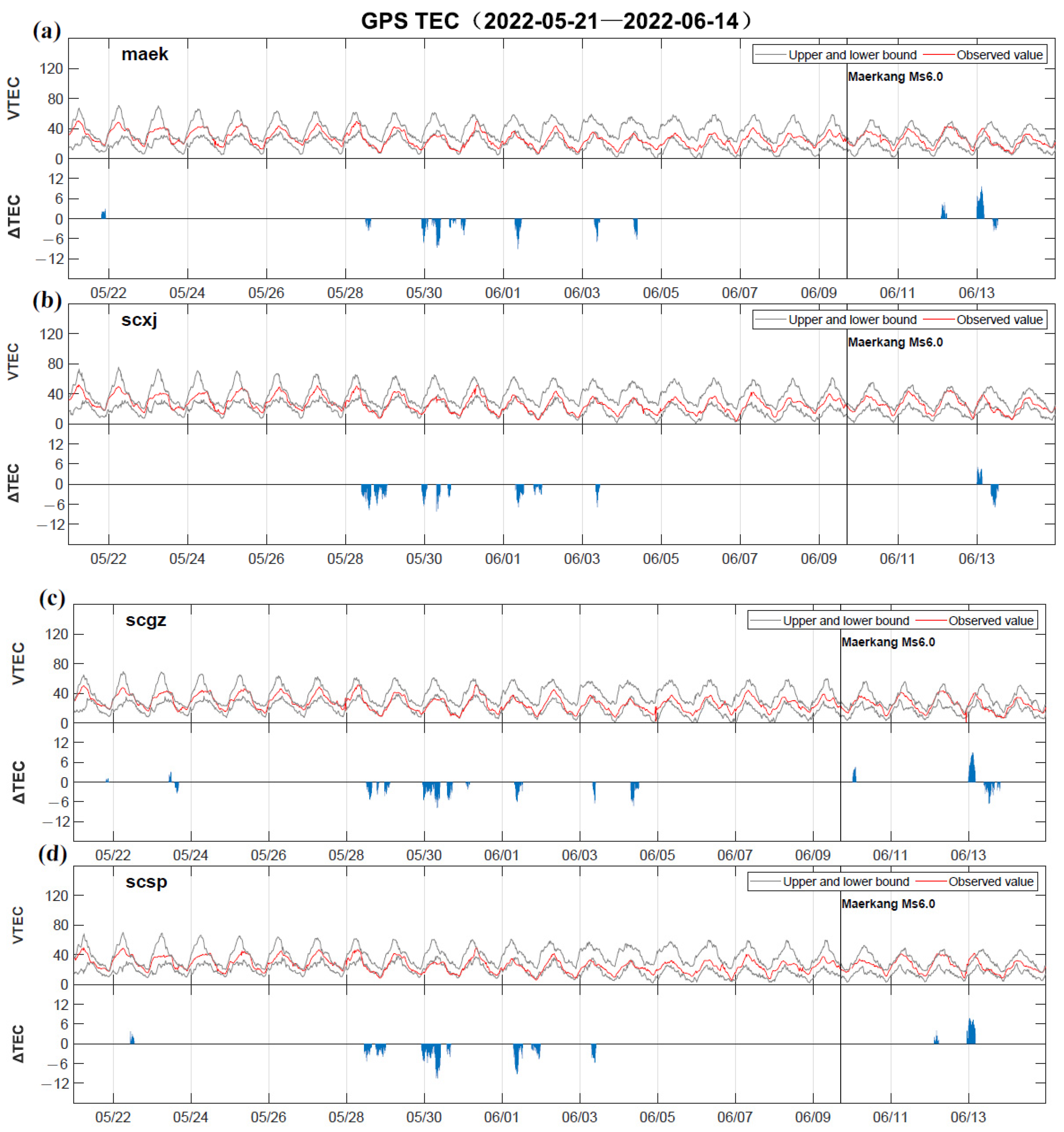
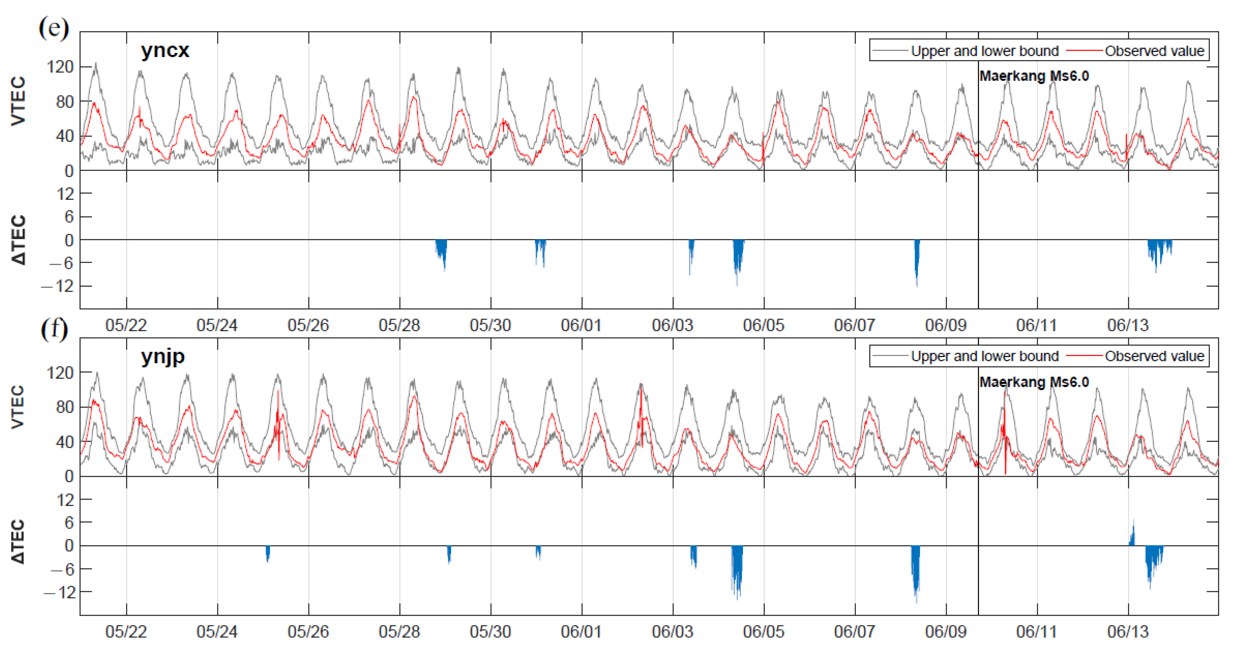
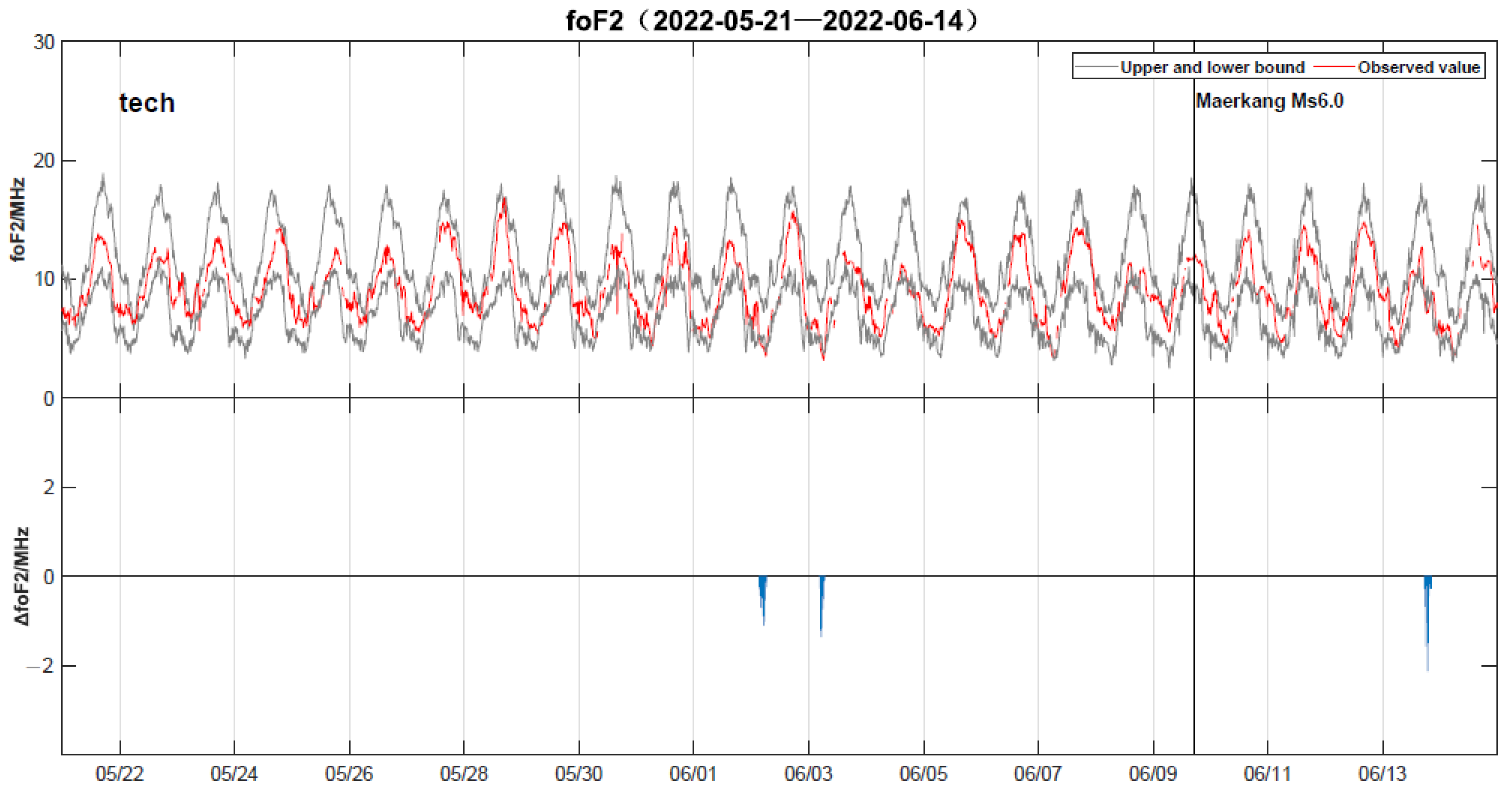
3.1. Analysis of Ground-Based Ionospheric Anomalies

In order to identify the spatial variations of anomalous signals on a global scale, we generated anomalous ionospheric distribution based on GIM data. Excluding the effect of solar-geomagnetic activity on anomalous ionospheric disturbances (Figure 1), it was found that the anomalous signals appeared on 1–4 June. As shown in Figure 3, each daily image contains 12 small images in a 2 h interval, the red star represents epicenter. On 1 June (Figure 3a), the magnitude of anomalous disturbances was strong globally, it may be influenced by the persistence of previous geomagnetic disturbances on 27–31 May. Then, the negative ionospheric anomalies appeared continuously on 2–4 June near the epicenter. On 2 June (Figure 3b), from 00:00–14:00 UT, significant negative ionospheric anomalies appeared globally, without spatial distribution characteristics related to the impending main shock. During 20:00–22:00 UT, negative ionospheric anomalies appeared near the epicenter and the abnormal amplitude was approximately −3TECu (1TECu = 10¹⁶ el/m²) [12]. On 3 June (Figure 3c), anomalous disturbances became more obvious from 00:00–10:00 UT, distributed above the epicenter at 08:00 and 10:00 UT, exceeding −5 TECu. On 4 June (Figure 3d), there were persistent anomalies above the epicenter at 08:00 and 10:00 UT, exceeding −5 TECu under quiet solar-geomagnetic conditions.

On the basis of the GIM analysis, the negative anomalies were detected on 2–4 June around the epicenter and its magnetic conjugate zone, revealing strong disturbances in ionosphere electron density during these days. The local characteristics of the ionospheric anomaly distribution were very obvious and consistent with the pre-seismic ionospheric anomaly changes.

In order to identify the anomalous disturbances on a small scale before earthquake, we analyzed temporal variations of GPS TEC and f_OF₂ in Sichuan and Yunnan regions. Since individual jump points can affect abnormal results, the abnormal signal judgment needs to meet the abnormal duration of more than 2 h in this paper.

The temporal variations of GPS TEC are shown in Figure 4, with the analysis period from 21 May to 14 June 2022. The red curve represents the observed value, the gray curve represents the upper and lower bounds, and the blue vertical line represents the abnormal value. It can be seen that the synchronous anomalies of multi-station were more obvious on 28, 30 May and 1, 3–4, 12–13 June. Comparing with the changes of solar-geomagnetic activity in this period (Figure 1), on 28, 30 May and 12–13 June, the ionospheric anomalies were mainly caused by active solar-geomagnetic conditions. On 1 June, the negative ionospheric anomalies were related to the persistent effects of previous geomagnetic disturbances. On 3 June, the anomalous disturbances were observed simultaneously by six GPS stations, reaching −6 TECu, while on 4 June, observed by four GPS stations, reaching −12 TECu.

On 3–4 June, the strong synchronous anomalies were found above the epicenter and surrounding stations under quiet solar-geomagnetic conditions. Both the temporal variations of GPS TEC and the anomalous distribution of GIM indicated that the anomalous disturbances may be caused by the seismic incubation process.

Meanwhile, the f_oF₂ temporal variations of the Tengchong vertical ionosonde station are shown in Figure 5, with the same anomaly extraction and determination rules for GPS TEC. As shown in Figure 5, ionospheric anomalies were more obvious on 2–3, 13 June. Under quiet solar-geomagnetic conditions, the negative anomalous disturbances appeared on 2–3 June before the earthquake, reaching −1.0 MHz and −1.4 MHz, respectively. The results of GIM and GPS TEC anomaly analysis were further verified.

Based on the ground-based ionospheric observations, the time-series data of stations have higher resolution, and the characteristics of pre-seismic anomalies are more obvious. Excluding the effects of solar-geomagnetic activity, the results of GIM, GPS TEC and f_OF₂ anomaly analysis all showed that the synchronous ionospheric disturbances occurred on 2–4 June around the epicenter, and the anomalous changes were consistent with the seismic and ionospheric coupling characteristics.

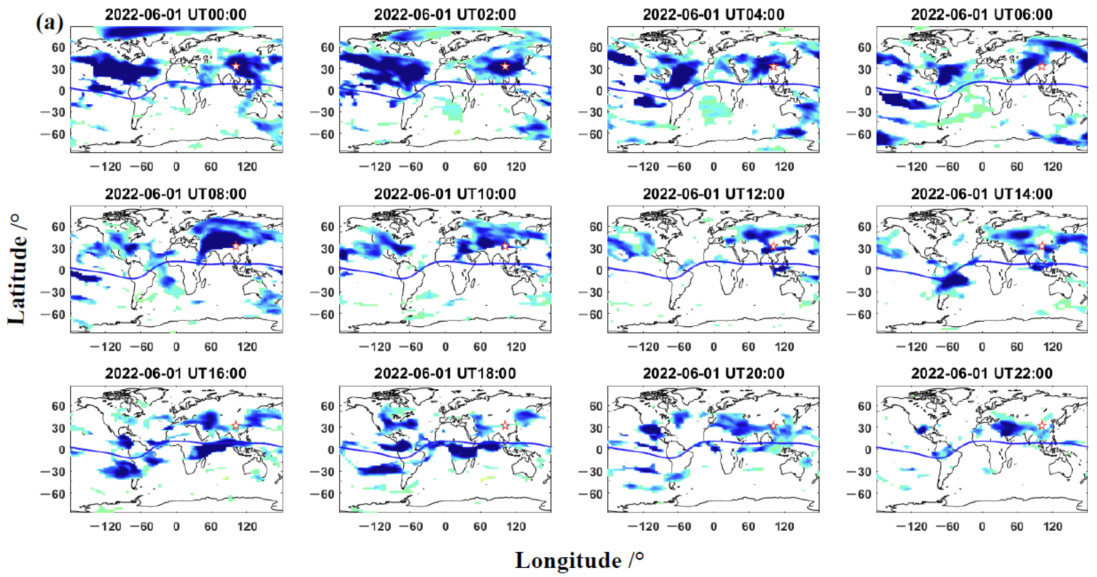
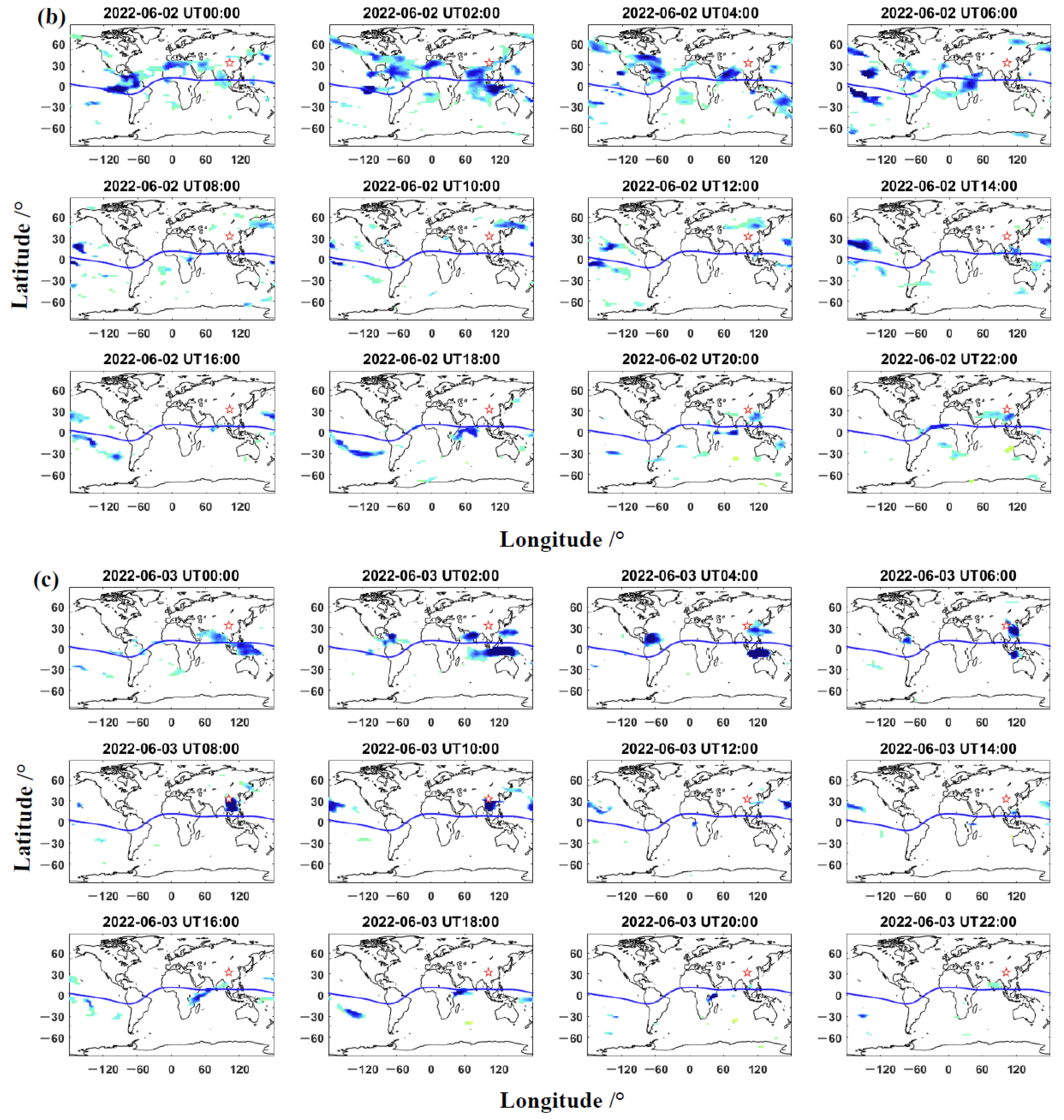
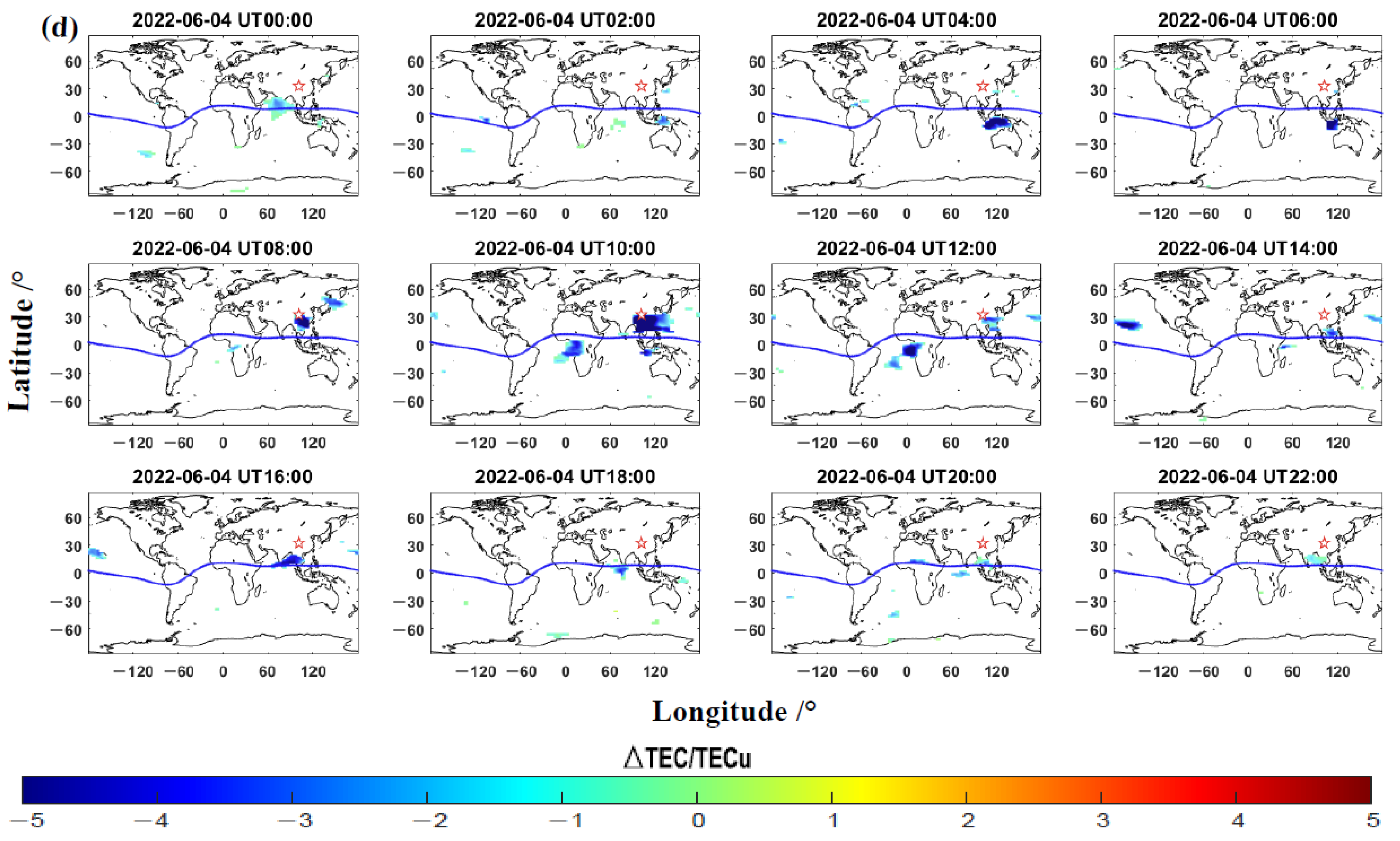
3.2. Analysis of CSES Ionospheric Anomalies

In order to further confirm ionospheric anomalies over the epicenter, a cross-validation analysis was also performed by using CSES data. The CSES orbital positions in the study area (20°~40° N, 92°~112° E) from 31 May to 4 June are shown in Figure 6, in which the observed data on 4 June are partially missing. As shown in Figure 6, the red star represents the epicenter, the red circle shows the seismogenic zones, approximately 380 km in radius according to the ‘train radius’ formula, ρ = 10^0.43M [41]. The average orbital longitude interval of CSES during the revisiting period is 4.8°, and one orbit will pass through the study area every day. Based on the CSES data, including Ne and Te parameters for the LAP, He⁺ and O⁺ density parameters for the PAP, we selected the nightside data and adopted the time-series method of revisiting orbit. The analysis period was from 21 May to 14 June 2022.

The temporal variations of Ne and Te are shown in Figure 7. The results show that synchronous abnormal disturbances of Ne and Te were obvious on 21, 29–30 May and 2 June. According to the variations of solar-geomagnetic activity (Figure 1), the anomalous disturbances on 21, 29–30 May were influenced by active solar-geomagnetic conditions. However, on 2 June, the synchronous negative anomalies of Ne and Te occurred around the epicenter area under quiet solar-geomagnetic conditions. ∆Ne dropped more than 5 $\times$ 10¹⁰ m⁻³, while ∆Te dropped more than 200 K. The synchronous variations of Ne and Te indicated that they may be affected by the same source of interference.

In addition, the temporal variations of He⁺ and O⁺ densities are shown in Figure 8. The results show that synchronous abnormal disturbances of He⁺ and O⁺ densities were obvious on 29 May and 1, 2, 4, 7, 10 June. With reference to the variations of solar-geomagnetic activity (Figure 1), the anomalous disturbances on 29 May and 7 June were influenced by active solar-geomagnetic conditions. Meanwhile, the anomalies on 1 June were associated with the persistent effects of previous geomagnetic disturbances analyzed above. However, the synchronous negative anomalies of He⁺ and O⁺ densities on 2, 4, 10 June can exclude the influence of solar-geomagnetic activity and exhibit consistent characteristics around the epicenter area. Among them, the most obvious synchronous anomalies were on 2 June, with ∆ He⁺ dropped more than 10¹⁰ m⁻³, while ∆ O⁺ dropped more than 3 × 10¹⁰ m⁻³. The synchronous anomalies were also detected on 4 June. Combining the results of the LAP and the PAP anomaly analysis, we found that the CSES multi-parameter showed significant anomalous disturbances before the earthquake, especially on 2, 4 June, and the anomaly distribution area was located right near the epicenter. The analysis results were generally consistent with the ground-based ionospheric observations.

Since the satellite orbits were far away from the epicenter on 3–4 June, and observed data were partially missing on 4 June, the satellite had insufficient ability to detect anomalies in the epicenter area. Based on the analysis results of ground-based and CSES data, excluding the effects of solar-geomagnetic activity, the ionospheric multi-parameter showed negative anomalous disturbances during 2–4 June. The local and synchronous characteristics of seismo-ionospheric disturbances were obvious 5–7 days before the earthquake. In general, the continuity and reliability of ground-based ionospheric data are relatively high. The reliability of the ionospheric anomaly identification can be effectively improved by the mutual verification of various ionospheric detection parameters.

4. Discussions

Seismo-ionospheric disturbances strongly associated with the Maerkang Ms6.0 earthquake swarm were analyzed in this paper. The temporal and spatial characteristics of ground-based and satellite ionospheric anomalies were very obvious on 2–4 June 2022. Actually, on 1 June 2022, another Ms6.1 earthquake that occurred in Lushan City approximately 250 km away from the epicenter of the Maerkang Ms6.0 earthquake swarm. Both earthquakes were caused by the push of the Bayan Har block to the southeast. The Maerkang earthquake swarm occurred near the Songgang fault inside the Aba secondary block in the east of Bayan Har block, while the seismogenic fault of the Lushan earthquake is the Shuangshi–Dachuan fault in the southern section of the Longmenshan fault zone [42]. The two seismic events do not constitute a correlation, and the Maerkang earthquake swarm is not an aftershock of the Lushan earthquake.

Through multi-parameter anomaly analysis, we found that significant ionospheric anomalies were observed on 17–18 May 2022 before the Lushan earthquake. The positive anomalies appeared near the epicenter under quiet solar-geomagnetic conditions which were probably caused by the Lushan earthquake. Nevertheless, although the negative anomalies during 2–4 June showed a strong correlation with the Maerkang earthquake swarm, it is still hard to confirm that the anomalies are not related to the Lushan earthquake. We expect to make new discoveries, but cannot distinguish between them yet. Furthermore, we found relatively strong ionospheric multi-parameter perturbations before the earthquake. Along with Ms5.8, the Ms6.0 and Ms5.2 earthquakes occurred on 9 June 2022 successively, the epicenters were all located in Caodeng Township. The stronger seismo-ionospheric coupling effect may be associated with this swarm-type earthquake.

In order to explain how earthquakes cause ionospheric anomalies, the study of the seismo-ionospheric coupling mechanism has been intensively developed. The lithosphere–atmosphere–ionosphere multi-channel coupling model is the most common explanation for seismo-ionospheric anomalies [26,27]. It mainly contains three channels: an overlapped DC electric field, an acoustic gravity wave and an electromagnetic wave. Among them, the overlapped DC electric field channel is relatively well developed, which can reasonably explain the whole process of propagation and coupling of seismo-ionospheric anomalies near the epicenter and its magnetic conjugate region. The model assumes that during earthquake incubation, the surface rock rupture under stress causes complex physicochemical reflections. A large number of additional ions are released, generating an anomalous surface atmospheric electrostatic field. Under certain conditions, the electrostatic field penetrates into the ionosphere and causes ionospheric anomalies [30,31,32,33]. The presences of an upward electrostatic field in the atmosphere before strong earthquakes are commonly reported in scientific experiments and actual observations [43,44,45,46,47,48]. Through the study of seismic events, Chen et al. [43] proposed a physical mechanism for the anomalous atmospheric electrostatic field under fair-weather condition, and the anomalous signals may be related to the occurrence of earthquakes. According to the study of Zhang et al. [47] around the Wenchuan Ms8.0 earthquake on 12 May 2008, the occurrence time of ionospheric disturbances was consistent with that of the abnormal electric field on the ground 1–2 days before the earthquake. Hao et al. [48] found that the anomalies in atmospheric electric fields appeared 2–40 days before the earthquakes.

In addition, the propagation of acoustic gravity waves in the atmosphere may also cause ionospheric anomalies. Scientists believe that near-surface macroscopic gases and heat sources generate acoustic gravity waves in the atmosphere and cause the enhancement of gravity and planetary waves. The propagation of these signals to the ionosphere then leads to anomalous oscillations in ionospheric temperature and density [26,27,28,49,50]. Based on the ionospheric disturbances observed by satellite at low and mid latitudes, Molchanov et al. [49] found that the anomalous energy originated from acoustic gravity waves. Piersanti et al. [50] tried to establish the propagation pathways of acoustic gravity waves in the atmosphere and ionosphere. Using the observations during the 5 August 2018 Bayan Earthquake, it was found that starting from the fault break, acoustic gravity waves were generated and mechanically perturbed the ionospheric plasma density before the earthquake. Furthermore, thermal infrared anomalies also occurred frequently before strong earthquakes. For some earthquake cases, brightness temperature increased with the growing near-surface heat sources before earthquakes [51,52,53,54]. Especially for the Maduo Ms7.4 earthquake on 21 May 2021, Qi et al. [51] have already observed the abnormal microwave brightness temperature occurred one to two months before the earthquake. Similarly, prior to the three strong earthquakes, 2008 Wenchuan Ms8.0, 2013 Lushan Ms7.0, and 2017 Jiuzhaigou Ms7.0, Jing et al. [53] illustrated that microwave brightness temperature anomalies appeared approximately two months before the three earthquakes, respectively.

Combining the above discussion and our analysis results, we suggest that the seismo-ionospheric coupling mechanism related to the Maerkang Ms6.0 earthquake swarm may be a combination of the above two coupling channels. This earthquake swarm activity was caused by the push of the Bayan Har block to the southeast. Prior to major earthquake, the critical change of the crusts in the region of epicenter leads to a great number of rocks being cracked and torn microscopically. A complex series of physico-chemical changes occur during the pre-seismic phase of a main shock. These changes, on the one hand, cause a growth of the atmospheric electrostatic field which penetrates into the ionosphere. The disturbed electric field can map from the epicenter along the earth’s magnetic field lines to the conjugate ionosphere, further affect the E × B drift and the equatorial plasma fountain [12,55,56]. Finally, ionospheric anomalies occur above the epicenter and its conjugate latitude. On the other hand, anomalous heat sources in the seismogenic zones generate acoustic gravity waves disturbances in the atmosphere and then cause the enhancement of gravity and planetary waves. As these signals propagate to the ionosphere, it causes anomalous oscillations in ionospheric temperature and density. Our Ne and Te analysis results also reflect these disturbances. However, there are few precursor monitoring stations near the epicenter, we could not verify whether the ionospheric disturbances are related to the anomalous changes of an atmospheric electrostatic field, near-surface macroscopic gases and heat sources, etc. We look forward to new discoveries.

According to the above analysis, to further test the reliability of ionospheric multi-parameter anomaly identification, we statistically analyzed the seismic events of magnitude 6 or above in the study area (20°~40° N, 92°~112° E) from 1 January 2019 to 1 July 2022. Based on the same anomaly extraction and determination rules, statistical results are summarized in

Table 2. Statistical table of seismo-ionospheric disturbances before nine earthquakes.

No.	EQ Date (UT)	EQ	Lat./°N	Lon./°E	Ms	Depth (km)	Abnormal Parameters	Abnormal Date	Pre EQ (DAY)
1	23 Apr 2019	Motuo, Tibet	28.4	94.61	6.3	10	fOF2, LAP (Ne, Te)	20 Apr 2019	−3
							GIM, GPS TEC, fOF2	21 Apr 2019	−2
2	17 Jun 2019	Changning, Sichuan	28.34	104.9	6	16	GIM, GPS TEC, fOF2, LAP (Ne, Te)	14 Jun 2019	−3
3	21 May 2021	Yangbi, Yunnan	25.67	99.87	6.4	8	GIM, GPS TEC, fOF2,	7 May 2021	−14
							GIM, GPS TEC, LAP (Ne, Te), PAP (He+, O+)	8 May 2021	−13
							GIM, GPS TEC, fOF2, LAP (Ne, Te), PAP (He+, O+)	9 May 2021	−12
4	21 May 2021	Maduo, Qinghai	34.59	98.34	7.4	17	GIM, GPS TEC, fOF2,	7 May 2021	−14
							GIM, GPS TEC, LAP (Ne, Te), PAP (He+, O+)	8 May 2021	−13
							GIM, GPS TEC, fOF2, LAP (Ne, Te), PAP (He+, O+)	9 May 2021	−12
5	15 Sep 2021	Luxian, Sichuan	29.2	105.34	6.0	10	GIM, GPS TEC, fOF2, LAP (Ne), PAP (He+, O+)	4 Sep 2021	−11
6	7 Jan 2022	Menyuan, Qinghai	37.77	101.26	6.9	12	GIM, GPS TEC, fOF2, LAP (Ne, Te), PAP (He+, O+)	23 Dec 2021	−15
							fOF2, LAP (Ne, Te), PAP (He+, O+)	24 Dec 2021	−14
							GIM, GPS TEC, fOF2, PAP (He+, O+)	26 Dec 2021	−12
7	25 Mar 2022	Delingha, Qinghai	38.5	97.33	6.0	10	fOF2, LAP (Ne), PAP (He+, O+)	22 Mar 2022	−3
							GIM, GPS TEC, LAP (Ne), PAP (He+, O+)	24 Mar 2022	−1
8	1 Jun 2022	Lushan, Sichuan	30.37	102.94	6.1	17	GIM, GPS TEC	17 May 2022	−14
							GIM, GPS TEC, fOF2	18 May 2022	−13
9	9 Jun 2022	Maerkang, Sichuan	32.25	101.82	6.0	13	GIM, GPS TEC, fOF2, LAP (Ne, Te), PAP (He+, O+)	2 Jun 2022	−7
							GIM, GPS TEC, fOF2	3 Jun 2022	−6
							GIM, GPS TEC, PAP (He+, O+)	4 Jun 2022	−5

, the occurrence times of all earthquakes are converted to Universal Time (UT). The results show that all 9 earthquakes are preceded by significant anomalous ionospheric disturbances. Except for the Lushan Ms6.1 earthquake in Sichuan Province on 1 June 2022, the anomalous changes of satellite parameters before the 8 earthquakes basically correspond to the ground-based parameters. In terms of the occurrence times, the anomalies are evident 1 to 15 days prior to the earthquakes. In terms of the observation parameters, the pre-seismic anomalies of GIM, GPS TEC and f_OF₂ show better consistency characteristics and higher anomaly detection capability. Meanwhile, the anomalous changes of He⁺ and O⁺ densities are consistent before the 6 earthquakes, with 12 anomalies, respectively (Figure 9). However, with a revisiting period of 5 days for CSES, the continuous observation capability in the same area is very limited and the detection of ionospheric anomalies is relatively poor. In addition, the statistical results show that the cumulative occurrence times of ionospheric anomalies before the Maduo Ms7.4 earthquake in Qinghai Province on 21 May 2021, the Menyuan Ms6.9 earthquake in Qinghai Province on 7 January, 2022, and the Maerkang Ms6.0 earthquake swarm in Sichuan Province on 9 June 2022 are all 3 days. The frequency of ionospheric anomalies is relatively high, which may be related to the magnitude of the earthquake and the intensity of the earthquake swarm.

From Table 2, we can also find that the pre-seismic anomalies of GIM, GPS TEC and f_OF₂ have better synchronous characteristics which may be related to the similarities of the detection parameters. Meanwhile, it is clear that before the earthquakes, there is a strong correlation between Ne and Te anomalies, with similarities between He⁺ and O⁺ density anomalies. These results are in good agreement with previous studies. For example, based on the Ne and Te data from DEMETER satellite, Liu et al. [57] studied ionospheric perturbations before 82 Ms ≥ 7.0 earthquakes during 2005–2010. It was found that Ne and Te showed synchronous anomalies before the strong earthquakes. Li et al. [58] statistically analyzed seismic influence on ionospheric parameters recorded by the CSES and DEMETER satellites. The analysis results showed that the correlation between O⁺ density and Ne anomalies was strong prior to the earthquakes, and the O⁺ density tended to be more sensitive to seismic activities than Ne. Obviously, it is an effective attempt to study the seismo-ionospheric coupling and coupling mechanism with multi-source data. In this paper, we found the characteristics of multi-parameter synchronous anomalies before the Maerkang Ms6.0 earthquake swarm. For CSES data, including Ne and Te parameters for the LAP and He⁺ and O⁺ density parameters for the PAP, at 19:00–20:00 UT on 2 June, between 20° and 30° N latitude, all parameters were characterized by synchronous changes and negative anomalies. The synchronous negative anomalies were also observed in the GIM southeast of the epicenter from ground-based data at the same time and location. Furthermore, there were persistent negative anomalies around the epicenter at 08:00–10:00 UT on 3–4 June observed in the GIM and GPS TEC. Due to the poor sustained observation capability of CSES in the same area, we were unable to obtain CSES observations for this time period. However, we did find the negative anomalies observed in the He⁺ and O⁺ densities around the epicenter at 19:00–20:00 UT on 4 June, between 30° and 40° N latitude, which may be correlated with the previous TEC anomalies. Multi-parameter anomalous perturbations were characterized by consistency and difference prior to the earthquake. The synchronous variations and correlations of multi-parameter can be considered as significant signals of upcoming main shock. For multi-parameter anomaly analysis, more seismic cases studies are needed, such as the disturbed time, spatial distribution, positive or negative correlations of multi-parameter anomalies. By enhancing the fusion of detection data and the understanding of the physical nature for multi-parameter, we can improve the effectiveness of multi-source data anomaly analysis and further promote the study of seismic ionospheric coupling.

In summary, based on the integrated ionospheric satellite–ground observations, the advantages of ground-based and satellite ionospheric detection techniques are given full play, and rich seismo-ionospheric anomalies are obtained. By analyzing the ionospheric multi-parameter anomaly characteristics and verifying each other from temporal and spatial scales, we can effectively improve the confidence level of anomaly identification and reduce the frequency of false anomalies. The orderly development of the CSES series satellites is expected to provide a network capability for three-dimensional observation in space, the study of seismo-ionospheric coupling mechanism will be further developed. We will have a more comprehensive understanding of seismo-ionospheric anomalies in the future.

5. Conclusions

In this paper, the seismo-ionospheric disturbances associated with the Maerkang Ms6.0 earthquake swarm were analyzed by the integrated ionospheric satellite–ground observations. We also statistically analyzed the seismic events of magnitude 6 or above in the study area since 2019, and mainly obtained the following conclusions.

The ground-based parameters GIM, GPS TEC, and f_OF₂, and the satellite parameters Ne, Te, He⁺ and O⁺ densities all showed negative anomalous disturbances on 2–4 June under quiet solar-geomagnetic conditions. Along with the anomalies of magnetic conjugate region, the local and synchronous characteristics of seismo-ionospheric disturbances were obvious 5–7 days before the Maerkang Ms6.0 earthquake swarm. Combining our analysis results, we suggest that the stronger seismo-ionospheric coupling effect probably be associated with this swarm-type earthquake, and the physical mechanism may be a combination of two coupling channels: an overlapped DC electric field and an acoustic gravity wave, as described by the lithosphere–atmosphere–ionosphere coupling (LAIC).

Next, based on the statistical analysis of seismic events in the study area since 2019, we found that the ground-based and satellite ionospheric anomalies were obvious with synchronous features prior to the strong earthquakes. The synchronous anomalies generally appeared 1–15 days before the earthquakes, and the continuity and reliability of ground-based ionospheric anomaly detection are relatively high.

Finally, according to the integrated ionospheric satellite–ground monitoring, the advantages of ground-based and satellite ionospheric detection techniques are given full play. Through the cross-validation analysis of multi-parameter, we can effectively improve the confidence level of anomaly identification and reduce the frequency of false anomalies. More detailed studies are needed to distinguish the seismo-ionospheric disturbances and fully understand the physical mechanism of the seismo-ionospheric coupling.

References

1. Liu, J.Y.; Chen, Y.I.; Pulinets, S.A.; Tsai, Y.B.; Chuo, Y.J. Seismo-ionospheric signatures prior to M ≥ 6.0 Taiwan earthquakes. Geophys. Res. Lett. 2000, 27, 3113–3116. [Google Scholar] [CrossRef]
2. Liu, J.Y.; Chuo, Y.J.; Shan, S.J.; Tsai, Y.B.; Chen, Y.I.; Pulinets, S.A.; Yu, S.B. Pre-earthquake ionospheric anomalies registered by continuous GPS TEC measurements. Ann. Geophys. 2004, 22, 1585–1593. [Google Scholar] [CrossRef] [Green Version]
3. Ahmed, J.; Shah, M.; Zafar, W.A.; Amin, M.A.; Iqbal, T. Seismoionospheric anomalies associated with earthquakes from the analysis of the ionosonde data. J. Atmos. Sol. Terr. Phys. 2018, 179, 450–458. [Google Scholar] [CrossRef]
4. Shah, M.; Inyurt, S.; Ehsan, M.; Ahmed, A.; Shakir, M.; Ullah, S.; Iqbal, M.S. Seismo ionospheric anomalies in Turkey associated with M ≥ 6.0 earthquakes detected by GPS stations and GIM TEC. Adv. Space Res. 2020, 65, 2540–2550. [Google Scholar] [CrossRef]
5. Le, H.; Liu, J.Y.; Liu, L. A statistical analysis of ionospheric anomalies before 736 M6.0+ earthquakes during 2002–2010. J. Geophys. Res. 2011, 116, A02303. [Google Scholar]
6. Marchetti, D.; De Santis, A.; Arcangelo, S.; Poggio, F.; Jin, S.; Piscini, A.A.; Campuzano, S. Magnetic Field and Electron Density Anomalies from Swarm Satellites Preceding the Major Earthquakes of the 2016–2017 Amatrice-Norcia (Central Italy) Seismic Sequence. Pure Appl. Geophys. 2020, 177, 305–319. [Google Scholar] [CrossRef]
7. Píša, D.; Parrot, M.; Santolík, O. Ionospheric density variations recorded before the 2010 Mw 8.8 earthquake in Chile. J. Geophys. Res. 2011, 116, A08309. [Google Scholar]
8. Parrot, M. Statistical analysis of automatically detected ion density variations recorded by DEMETER and their relation to seismic activity. Ann. Geophys. 2012, 55, 149–155. [Google Scholar]
9. Liu, J.Y.; Chen, Y.I.; Chuo, Y.J.; Tsai, H.F. Variations of ionospheric total electron content during the Chi-Chi earthquake. Geophys. Res. Lett. 2001, 28, 1381–1386. [Google Scholar] [CrossRef] [Green Version]
10. Liu, J.Y.; Chen, Y.I.; Chen, C.H.; Liu, C.Y.; Chen, C.Y.; Nishihashi, M.; Li, J.Z.; Xia, Y.Q.; Oyama, K.I.; Hattori, K.; et al. Seismoionospheric GPS total electron content anomalies observed before the 12 May 2008 Mw7.9 Wenchuan earthquake. J. Geophys. Res. 2008, 114, A04320. [Google Scholar]
11. Chuo, Y.J.; Chen, Y.I.; Liu, J.Y.; Pulinets, S.A. Ionospheric foF2 vaiations prior to strong earthquakes in Taiwan area. Adv. Space Res. 2001, 27, 1305–1310. [Google Scholar] [CrossRef]
12. Liu, J.; Wang, W.; Zhang, X.; Wang, Z.; Zhou, C. Ionospheric total electron content anomaly possibly associated with the April 4, 2010 Mw7.2 Baja California earthquake. Adv. Space Res. 2022, 69, 2126–2141. [Google Scholar] [CrossRef]
13. Zhong, M.; Shan, X.; Zhang, X.; Qu, C.; Guo, X.; Jiao, Z. Thermal Infrared and Ionospheric Anomalies of the 2017 Mw6.5 Jiuzhaigou Earthquake. Remote Sens. 2020, 12, 2843. [Google Scholar] [CrossRef]
14. Zhu, F.; Wu, Y.; Lin, J.; Zhou, Y.; Xiong, J.; Yang, J. Anomalous response of ionospheric VTEC before the Wenchuan earthquake. Acta Seismologica 2009, 31, 180–187. [Google Scholar]
15. Parrot, M. Statistical analysis of the ion density measured by the satellite DEMETER in relation with the seismic activity. Earthq. Sci. 2011, 24, 513–521. [Google Scholar] [CrossRef]
16. Zhang, X.; Fidani, C.; Huang, J.; Shen, X.; Zeren, Z.; Qian, J. Burst increases of precipitating electrons recorded by the DEMETER satellite before strong earthquakes. Nat. Hazards Earth Syst. Sci. 2013, 13, 197–209. [Google Scholar] [CrossRef] [Green Version]
17. De Santis, A.; Marchetti, D.; Spogli, L.; Cianchini, G.; Pavon-Carrasco, F.J.; De Franceschi, G.; Di Giovambattista, R.; Perrone, L.; Qamili, E.; Cesaroni, C.; et al. Magnetic Field and Electron Density Data Analysis from Swarm Satellites Searching for Ionospheric Effects by Great Earthquakes: 12 Case Studies from 2014 to 2016. Atmosphere 2019, 10, 371. [Google Scholar] [CrossRef] [Green Version]
18. Parrot, M.; Li, M. DEMETER results related to seismic activity. Ursi Radio Sci. Bull. 2017, 88, 18–25. [Google Scholar]
19. Li, M.; Parrot, M. Statistical analysis of the ionospheric ion density recorded by DEMETER in the epicenter areas of earthquakes as well as in their magnetically conjugate point areas. Adv. Space Res. 2018, 61, 974–984. [Google Scholar] [CrossRef]
20. Yan, R.; Parrot, M.; Pinçon, J.L. Statistical study on variations of the ionospheric ion density observed by DEMETER and related to seismic activities. J. Geophys. Res. Space Phys. 2017, 122, 12421–12429. [Google Scholar] [CrossRef] [Green Version]
21. Li, M.; Wang, H.; Liu, J.; Shen, X. Two Large Earthquakes Registered by the CSES Satellite during Its Earthquake Prediction Practice in China. Atmosphere 2022, 13, 751. [Google Scholar] [CrossRef]
22. Du, X.; Zhang, X. Ionospheric Disturbances Possibly Associated with Yangbi Ms6.4 and Maduo Ms7.4 Earthquakes in China from China Seismo Electromagnetic Satellite. Atmosphere 2022, 13, 438. [Google Scholar] [CrossRef]
23. Zhang, X.; Dong, L.; Nie, L. The Ionospheric Responses from Satellite Observations within Middle Latitudes to the Strong Magnetic Storm on 25–26 August 2018. Atmosphere 2022, 13, 1271. [Google Scholar] [CrossRef]
24. Akhoondzadeh, M.; Parrot, M.; Saradjian, M.R. Electron and ion density variations before strong earthquakes (M > 6.0) using DEMETER and GPS data. Nat. Hazards Earth Syst. Sci. 2010, 10, 7–18. [Google Scholar] [CrossRef] [Green Version]
25. Zhang, X.; Wang, Y.; Boudjada, M.; Liu, J.; Magnes, W.; Zhou, Y.; Du, X. Multi-Experiment Observations of Ionospheric Disturbances as Precursory Effects of the Indonesian Ms6.9 Earthquake on 5 August 2018. Remote Sens. 2020, 12, 4050. [Google Scholar] [CrossRef]
26. Hayakawa, M. Electromagnetic phenomena associated with earthquakes: A frontier in terrestrial electromagnetic noise environment. Recent Res. Dev. Geophys. 2004, 6, 81–112. [Google Scholar]
27. Molchanov, O.; Fedorov, E.; Schekotov, A.; Gordeev, E.; Chebrov, V.; Surkov, V.; Rozhnoi1, A.; Andreevsky, S.; Iudin, D.; Yunga, S.; et al. Lithosphere-atmosphere-ionosphere coupling as governing mechanism for preseismic short-term events in atmosphere and ionosphere. Nat. Hazards Earth Syst. Sci. 2004, 4, 757–767. [Google Scholar] [CrossRef]
28. Kamogawa, M. Preseismic lithosphere-atmosphere-ionosphere coupling. Eos Trans. Am. Geophys. Union 2014, 87, 417–424. [Google Scholar] [CrossRef] [Green Version]
29. Pulinets, S.A.; Boyarchuk, K. Ionospheric Precursors of Earthquakes; Springer: Berlin/Heidelberg, Germany, 2004; pp. 75–169. [Google Scholar]
30. Pulinets, S.A.; Ouzounov, D. Lithosphere–Atmosphere–Ionosphere Coupling (LAIC) model—An unified concept for earthquake precursors validation. J. Asian Earth Sci. 2011, 41, 371–382. [Google Scholar] [CrossRef]
31. Pulinets, S.A.; Boyarchuk, K.; Hegai, V.V. Quasielectrostatic model of atmosphere-thermosphere-ionosphere coupling. Adv. Space Res. 2000, 26, 1209–1218. [Google Scholar] [CrossRef]
32. Sorokin, V.M.; Chmyrev, V.M.; Yaschenko, A.K. Theoretical model of DC electric field formation in the ionosphere stimulated by seismic activity. J. Atmos. Sol.-Terr. Phys. 2005, 67, 1259–1268. [Google Scholar] [CrossRef]
33. Sorokin, V.M.; Yaschenko, A.K.; Hayakawa, M. A perturbation of DC electric field caused by light ion adhesion to aerosols during the growth in seismic-related atmospheric radioactivity. Nat. Hazards Earth Syst. Sci. 2007, 7, 155–163. [Google Scholar] [CrossRef]
34. Wu, L.X.; Qin, K.; Liu, S.J. GEOSS-based thermal parameters analysis for earthquake anomaly recognition. Proc. IEEE 2012, 100, 2891–2907. [Google Scholar] [CrossRef]
35. Zhang, X.; Shen, X. The development in seismo-ionospheric coupling mechanism. Prog. Earthq. Sci. 2022, 52, 193–202, (In Chinese with an English abstract). [Google Scholar]
36. Xiong, B. Ionospheric Response to Solar Flare and GPS-TEC Monitoring. Ph.D. Thesis, Institute of Geology and Geophysics, Chinese Academy of Sciences, Beijing, China, May 2012. [Google Scholar]
37. Chen, Y.I.; Chuo, J.Y.; Liu, J.Y.; Puilnets, S.A. A Statistical Study of Ionospheric Precursors of Strong Earthquake at Taiwan Area, XXIVth General Ass.; URSI: Paris, France, 1999; p. 745. [Google Scholar]
38. Xie, T.; Chen, B.; Wu, L.; Dai, W.; Kuang, C.; Miao, Z. Detecting seismo-ionospheric anomalies possibly associated with the 2019 Ridgecrest (California) earthquakes by GNSS, CSES, and Swarm observations. J. Geophys. Res. Space Phys. 2021, 126, e2020JA028761. [Google Scholar] [CrossRef]
39. Dong, Y.; Gao, C.; Long, F.; Yan, Y. Suspected Seismo-Ionospheric Anomalies before Three Major Earthquakes Detected by GIMs and GPS TEC of Permanent Stations. Remote Sens. 2022, 14, 20. [Google Scholar] [CrossRef]
40. Tao, D.; Wang, G.; Zong, J.; Wen, Y.; Cao, J.; Battiston, R.; Zeren, Z. Are the Significant Ionospheric Anomalies Associated with the 2007 Great Deep-Focus Undersea Jakarta–Java Earthquake? Remote Sens. 2022, 14, 2211. [Google Scholar] [CrossRef]
41. Dobrovolsky, I.P.; Zubkov, S.I.; Miachkin, V.I. Estimation of the Size of Earthquake Preparation Zones. Pure Appl. Geophys. 1979, 117, 1025–1044. [Google Scholar] [CrossRef]
42. Zhang, J.Y.; Dai, D.Q.; Yang, Z.G.; Xi, N.; Deng, W.Z.; Xu, T.R.; Sun, L. Preliminary Analysis of Emergency Production and Source Parameters of the M6.0 Earthquake on June 10, 2022 in Maerkang City, Sichuan Province. Earthq. Res. China 2022, 38, 370–382, (In Chinese with an English abstract). [Google Scholar]
43. Chen, T.; Zhang, X.; Zhang, X.; Jin, X.; Wu, H.; Ti, S.; Li, R.; Li, L.; Wang, S. Imminet estimation of earthquake hazard by regional network monitoring the near surface vertical atmospheric electrostatic field. Chinese. J. Geophys. 2021, 64, 1145–1154, (In Chinese with an English abstract). [Google Scholar]
44. Zhou, C.; Liu, Y.; Zhao, S.; Liu, J.; Zhang, X.; Huang, J.; Shen, X.; Ni, B.; Zhao, Z. An electric field penetration model for seismo-ionospheric research. Adv. Space Res. 2017, 60, 2217–2232. [Google Scholar] [CrossRef]
45. Smirnov, S. Association of the negative anomalies of the quasistaticelectric field in atmosphere with Kamchatka seismicity. Nat. Hazards Earth Syst. Sci. 2008, 8, 745–749. [Google Scholar] [CrossRef]
46. Choudhury, A.; Guha, A.; De, B.K.; Roy, R. A statistical study on precursory effects of earthquakes observed through the atmospheric vertical electric field in northeast India. Ann. Geophys. 2013, 56, 1861–1867. [Google Scholar]
47. Zhang, X.; Chen, H.; Liu, J.; Shen, X.; Miao, Y.; Du, X.; Qian, J. Ground-based and satellite DC-ULF electric field anomalies around Wenchuan M8.0 earthquake. Adv. Space Res. 2012, 50, 85–95. [Google Scholar] [CrossRef]
48. Hao, J.; Tang, T.; Li, D. Advancement of the study on taking the anomalies of static atmospheric field as index of short-term and imminent earthquake prediction. Earthquake 1998, 18, 245–256. [Google Scholar]
49. Molchanov, O.A. On the origin of low-and middler-latitude ionospheric turbulence. Phys. Chem. Earth 2004, 9, 559–567. [Google Scholar] [CrossRef]
50. Piersanti, M.; Materassi, M.; Battiston, R. Magnetospheric-ionospheric-lithospheric coupling model. Observations during the 5 August 2018 Bayan earthquake. Remote Sens. 2020, 12, 3299. [Google Scholar] [CrossRef]
51. Qi, Y.; Wu, L.; Ding, Y.; Liu, Y.; Chen, S.; Wang, X.; Mao, W. Extraction and Discrimination of MBT Anomalies Possibly Associated with the Mw 7.3 Maduo (Qinghai, China) Earthquake on 21 May 2021. Remote Sens. 2021, 13, 4726. [Google Scholar] [CrossRef]
52. Takashi, M.; Takano, T. Detection algorithm of earthquake-related rock failures from satellite-borne microwave radiometer data. IEEE Trans. Geosci. Remote Sens. 2010, 48, 1768–1776. [Google Scholar]
53. Jing, F.; Singh, R.P.; Cui, Y.; Sun, K. Microwave brightness temperature characteristics of three strong earthquakes in Sichuan province, China. IEEE J. Sel. Topics Appl. Earth Observ. Remote Sens. 2020, 13, 513–522. [Google Scholar] [CrossRef]
54. Jing, F.; Singh, R.P.; Sun, K.; Shen, X. Passive microwave response associated with two main earthquakes in Tibetan Plateau, China. Adv. Space Res. 2018, 62, 1675–1689. [Google Scholar] [CrossRef]
55. Liu, J.Y.; Le, H.; Chen, Y.I.; Chen, C.H.; Liu, L.; Wan, W.; Su, Y.Z.; Sun, Y.Y.; Lin, C.H.; Chen, M.Q. Observations and simulations of seismoionospheric GPS total electron content anomalies before the 12 January 2010 M7 Haiti earthquake. J. Geophys. Res. 2011, 116, A04302. [Google Scholar]
56. Liu, J.Y.; Chen, C.H.; Chen, Y.I.; Yang, W.H.; Oyama, K.I.; Kuo, K.W. A statistical study of ionospheric earthquake precursors monitored by using equatorial ionization anomaly of GPS TEC in Taiwan during 2001–2007. J. Asian Earth Sci. 2010, 39, 76–80. [Google Scholar] [CrossRef]
57. Liu, J.; Huang, J.P.; Zhang, X.M. Ionospheric perturbations in plasma parameters before global strong earthquakes. Adv. Space Res. 2014, 53, 776–787. [Google Scholar] [CrossRef]
58. Li, M.; Shen, X.; Parrot, M.; Zhang, X.; Zhang, Y.; Yu, C.; Yan, R.; Liu, D.; Lu, H.; Guo, F.; et al. Primary joint statistical seismic influence on ionospheric parameters recorded by the CSES and DEMETER satellites. J. Geophys. Res. Space Phys. 2020, 125, e2020JA028116. [Google Scholar] [CrossRef]
Figure 1. Daily variation of F10.7, Kp, Dst and AE indices, where (ad) denote F10.7, Kp, Dst, and AE indices, respectively. In each figure, the black line indicates the time of the Maerkang Ms6.0 earthquake, and the red line indicates threshold value of each index.
Atmosphere 13 01745 g001
Figure 2. Distribution of epicenter and stations. The red star represents epicenter, green triangle and blue circle represent GPS and vertical ionosonde stations, respectively.
Atmosphere 13 01745 g002
Figure 3. Anomalous distribution of GIM, where (ad) denote the daily variation from 1 June to 4 June 2022. Each daily image contains 12 small images in a 2 h interval, the red star represents the epicenter, the blue line is the magnetic equator and UT is shown as the title on each panel.
Atmosphere 13 01745 g003aAtmosphere 13 01745 g003bAtmosphere 13 01745 g003c
Figure 4. Temporal variations of GPS TEC from six GPS stations in and around the epicenter. (a) Maerkang station, (b) Xiaojin station, (c) Ganzi station, (d) Songpan station, (e) Chuxiong station, and (f) Jinping station. The time of earthquake is annotated by the black line, the upper and lower bounds are shown in gray, and observed values are shown in red. The abnormal values are shown in blue, represented as ∆TEC.
Atmosphere 13 01745 g004aAtmosphere 13 01745 g004b
Figure 5. Temporal variations of fOF2 from the Tengchong vertical ionosonde station. The time of earthquake is annotated by the black line, the upper and lower bounds are shown in gray, and observed values are shown in red. The abnormal values are shown in blue, represented as ∆fOF2.
Atmosphere 13 01745 g005
Figure 6. CSES orbital positions in the study area from 31 May to 4 June. The blue line represents the orbit of CSES in the nighttime, the red star represents the epicenter, the red circle shows the seismogenic zones (approximately 380 km in radius).
Atmosphere 13 01745 g006
Figure 7. Temporal variations of Ne and Te. (a) Ne; (b) Te. The upper and lower bounds are shown in gray, and observed values are shown in red. The abnormal values are shown in blue, represented as ∆Ne and ∆Te.
Atmosphere 13 01745 g007
Figure 8. Temporal variations of He+ and O+ densities. (a) He+ density; (b) O+ density. The upper and lower bounds are shown in gray, and observed values are shown in red. The abnormal values are shown in blue, represented as ∆ He+ and ∆ O+.
Atmosphere 13 01745 g008
Figure 9. Abnormal test results for observation parameters. The blue bar represents seismic events, and the red bar represents abnormal frequency.
Atmosphere 13 01745 g009