Article

Analysis of Cooling and Humidification Effects of Different Coverage Types in Small Green Spaces (SGS) in the Context of Urban Homogenization: A Case of HAU Campus Green Spaces in Summer in Zhengzhou, China

1
Department of Landscape Planning and Regional Development, Faculty of Landscape Architecture and Urbanism, Szent István University, 1118 Budapest, Hungary
2
Department of Landscape Architecture, College of Landscape Architecture and Art, Henan Agricultural University, Zhengzhou 450002, China
3
CMA Henan Key Laboratory of Agrometeorological Support and Applied Technique, Zhengzhou 450003, China
4
Henan Provincial Climate Centre, Zhengzhou 450003, China
5
Department of Climatology and Landscape Ecology, University of Szeged, 6722 Szeged, Hungary
*
Authors to whom correspondence should be addressed.
These authors contributed equally to this work.
Atmosphere 2020, 11(8), 862; https://doi.org/10.3390/atmos11080862
Submission received: 29 June 2020 / Revised: 2 August 2020 / Accepted: 12 August 2020 / Published: 14 August 2020
(This article belongs to the Special Issue Interaction between Urban Microclimates and the Buildings)

Abstract

:
In the context of global warming, more and more cities are experiencing extreme Urban Heat Island (UHI) effects and extreme weather phenomena, but urban green spaces are proven to mitigate UHI. Most of UHI’s research focuses on the large scale and uses remote sensing methods, which do not reflect the dynamic characteristics in detail and do not detect internal influencing factors of the green space cooling effect. Therefore, this study focused on Small Green Spaces (SGS), carrying out the measurement of the meteorological parameters (temperature, relative humidity, wind direction, wind speed, photosynthetic radiation) of the 16 sites in four types of coverage (Impervious surface; Shrub-grass; Tree-grass; Tree-shrub-grass) in a university campus. At the same time, the coverage characteristic parameters, such as Canopy Density (CD), Leaf Area Index (LAI), Photosynthetically Active Radiation (PAR), Mean Leaf Angle (MLA), of each plot were analyzed and compared. The results showed that there were significant differences in temperature among different coverage types in SGS. The biggest difference was concentrated in the noon period when solar radiation is strongest during the day. The difference between the four types of coverage with vegetation at night was small. The maximum air temperature difference among the four types could reach 8.9 ℃ and the maximum relative humidity difference was 28.5%. The cooling effect of the multi-layer vegetation-covered (Tree-shrub-grass) area was the largest compared to the impervious surface, indicating that tree cover was the core factor affecting the temperature. Temperature and relative humidity had a close correlation with surface coverage types and some plant community characteristics (such as CD and LAI). The cooling and humidifying effects of plants were also related to PAR and leaf angle. The results provide suggestions for green space management and landscape design.

1. Introduction

Rapid urbanization has changed the structure of urban surfaces. According to statistics, more than 50% of the global population is urban; it is estimated that by 2050, the proportion of the urban population will exceed 66% [1]. Urban areas are the center of human activities, energy consumption, and greenhouse gas emissions, which contribute to global climate change. Most of the cities are located in plains at lower elevations [2]. Due to the composition of the underlying surfaces of the city (urban roughness) such as impervious surfaces, buildings, and municipal facilities [3], have led to a change in the local climate that has resulted in problems such as urban heat island effects [4]. Local climate change is caused by two different but related reasons. One of them includes surface cover, building materials and building forms [5]. The other one is anthropogenic activities, such as industrialization, transportation, solid waste generation, and excess waste-water generation, which have also been reported to influence the natural structure of cities [6]. The urban form also has an impact on urban heat island, as many researchers have demonstrated this [7,8]. Due to the lack of consideration on the relations between urban forms and urban ventilation in city planning, the urban ventilation environment is getting worse and worse, hence, increasing the intensity of the heat island effect. This drawback forms the backbone of enormous research interest in the adjustment of urban form and urban function, especially adjusting the microclimate to mitigate the heat island effect.
Urban heat island (UHI) was first discovered by Luke Howard in 1818, which refers to the phenomenon that cities are warmer than surrounding rural areas [9]. From then, UHI effects have been studied over the last two centuries. Generally, the traditional heat island measurement is called “canopy layer urban heat island”, which exists in the layer where people live, from the ground to below the tops of trees and roofs [10]. This shows that the urban heat island is obtained from the measurement of the air temperature in the city. Because the air is flowing and transparent, there is no effective recording method to indicate its spatial state. Most scholars study the urban heat island effect by using satellites [11,12,13,14,15,16]. The surface temperature obtained from the image needs to be calibrated. Although there is a certain relationship between the surface temperature and the air temperature, this relationship becomes extremely uncertain due to the heterogeneity of the surface. Furthermore, human thermal comfort is related to air temperature, mean radiant temperature, wind speed and relative humidity [17,18], thus, studying the characteristics of microclimate at the city scale is more conducive to interfacing with urban planning. From the thermal conduction studies, the simulation method was commonly used to investigate with a different scale. For example, the Urban Weather Generator (UWG) model was mainly applied to simulate the local microclimatic phenomena in the city scale [19]. In the mesoscale weather simulation, the Computational Fluid Dynamics (CFD) model was widely used to estimate the thermal conduction and heat flux in city areas such as buildings and street levels [20,21].
Urban cool island (UCI) usually refers to the areas that have a lower temperature compared with their surroundings such as vegetation areas and water bodies in cities [22,23]. Vegetation changes the three-dimensional space of the city seasonally and also changes the incident and reflected energy of the sun. Vegetation cools down the air and surfaces through evapotranspiration and shadows. Soil and water use their own absorption and high heat capacity to achieve the cooling effect [24]. In addition to the physical properties of the above-mentioned and other urban constituent materials, the impact of green space layout is also proven [25,26]. At present, there are two main scales for studying the cooling effect of urban green space (UGS): one is large-scale research based on satellite imagery and meteorological data [27,28,29]; these studies applied indicators such as park cooling intensity (PCI) and green space cooling intensity (GCI) to quantify the cooling effect of UGS [22,30,31]. The other one is small-scale research through field observation and application of models [17,32,33]. Field observation data can more directly and accurately characterize the dynamic relationship between urban green space and atmospheric temperature than other spatial datasets derived from satellite imagery. This approach, at this scale, has an important practical guiding significance for the rational planning and layout of urban green space. Compared with the large-scale landscape design, the small-scale design is easier to manage. The SGSs like cells in the city play an important role in regulating the microclimate [34]. Specifically, they play a significant role in improving the environmental quality of local microclimate. However, the role played by SGSs has often been neglected in research.
This article is in the context of the rapid spread of global urbanization. A series of urban homogenization symptoms continue to be unraveled [35,36,37], for instance, a study shows that urban plant communities from 35 Chinese cities had lower dissimilarities of species composition between urban areas than these of plant communities in natural areas. More specifically, plant species from families like Prunus, Populus, and Magnolia have contributed to the homogenization of urban woody plants, due to their wide use in landscaping during the rapid urbanization [38]. Another study also showed that China’s urban plant communities are becoming homogenized, as urban communities of different cities are highly similar to each other despite the geographical separation [39]. Green spaces in different cities often exist with the same plant communities, hence, it is of universal significance to study a certain type of green space. Traditional studies on urban thermal environments focused on large-scale ranges [40], these studies used satellite images with low resolution which were unable to identify small-scale complex factors, and could not reflect the hourly changes in urban thermal environment. From this perspective, this article employed SGS as study areas and applied related instruments to quantify and explore the impact of different coverage types on the thermal environment, with an outlook towards future small-scale landscape design.
In this study, the time was selected in the hot and dry summer of August 2019, and the study area was selected in the green spaces of a university campus. The research object includes four differently coverage surface types in four green spaces, canopy and vegetation parameters in 16 spots were quantified by instruments. The thermal performance of the coverage type and its impact on the meteorological parameters were analyzed and compared. The intrinsic influencing factors for the regulation effect of green spaces on microclimate were also conducted. This is also a topic of practical significance in the context of reducing UHI.
The objectives of this study were:
  • To study the spatiotemporal microclimatic characteristics of different types of green spaces types on hot and dry summer days.
  • To analyze and compare different surface coverage types of SGS on microclimate.
  • To analyze the relationship between microclimatic and coverage characteristics (vegetation structure, coverage attributes, leaf area index, leaf angle, photosynthetic radiation) of the green space.

2. Materials and Methods
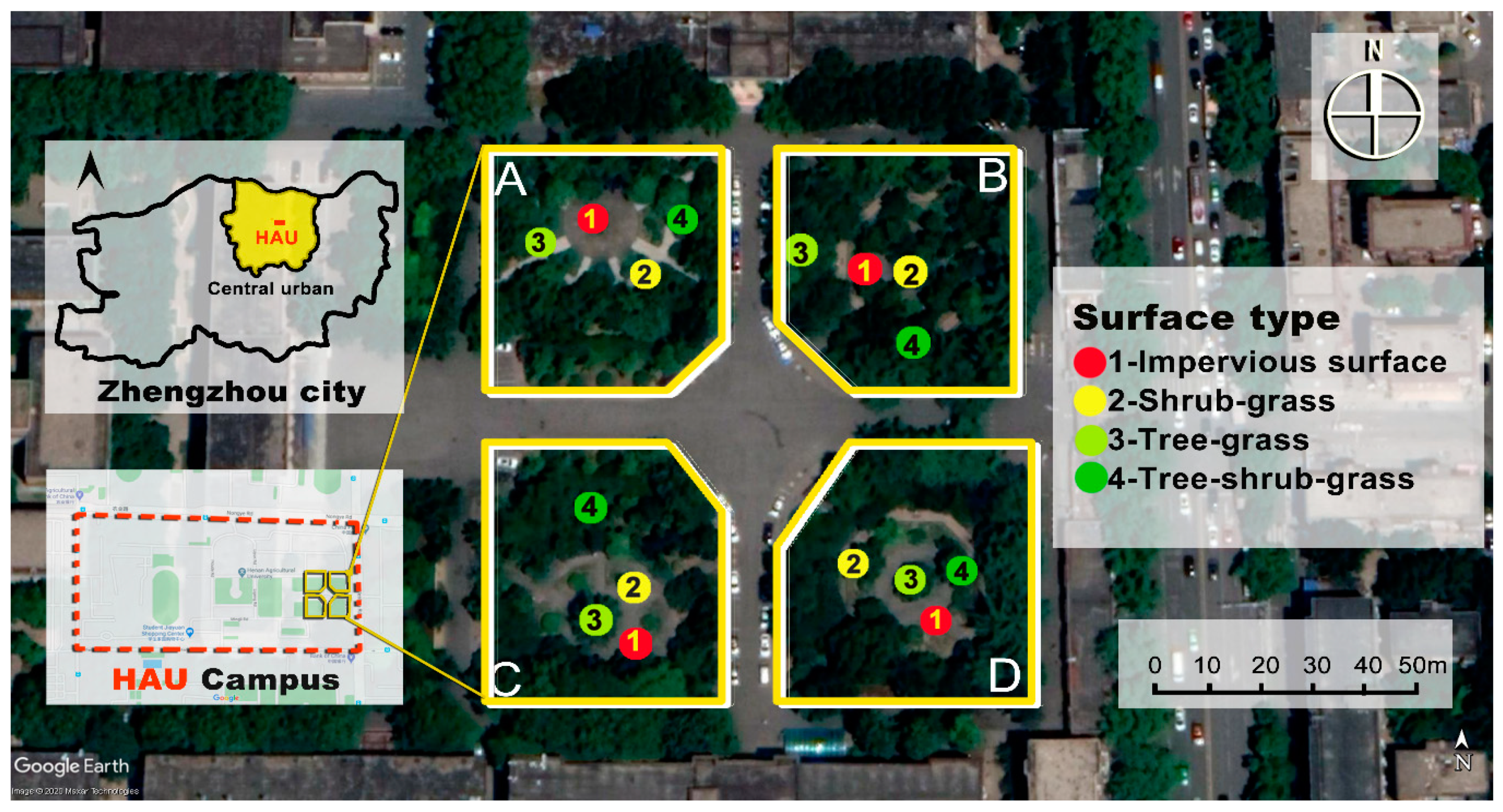
2.1. Study Area

This study was undertaken in Zhengzhou (34°160 N–34°580 N, 112°420 E–114°140 E), the capital city of Henan province in central China. It located the north China plain and close to the Yellow River. The city is one of the largest transportation hubs in China. The population of the city was approximately 9.56 million according to the 2018 census [41]. The population density (1390/km2) is the second-highest in China. Zhengzhou lies in a dry-winter humid subtropical climate zone according to the Köppen climate classification system [42]. The annual average temperature was 15.6 ℃; August was the hottest, with a monthly average temperature of 25.96 ℃; January was the coldest, with a monthly average temperature of 2.156 ℃. The annual average rainfall was 542.15 mm [41].
The research plot was selected on the campus of Henan Agricultural University (HAU) in Jinshui district, within Zhengzhou city. The entire campus is about 23 ha. The sample area is located on the east side of the campus, next to the east gate (Figure 1). Garden A, B, C and D are 0.21 ha; 0.26 ha; 0.23 ha and 0.25 ha, respectively. These gardens are surrounded by teaching and learning buildings. The average height of the surrounding buildings is about 18 m, so the energy exchange with the surrounding was relatively weak compared with the area with no surrounded by buildings.
In addition to providing leisure spaces for teachers and students, the four selected campus green spaces are also the experimental bases for the teaching of landscape architecture. Each garden has open spaces and different vegetation coverage types. The four gardens are mainly composed of evergreen plants (such as Cedrus deodara, Ligustrum compactum, Buxus mollicula, etc.), deciduous plants (Platanus orientalis Linn., Cinnamomum camphora; Bischofia javanica, Salix babylonica, Styphnolobium japonicum, Magnolia denudata, etc.), shrub (Fatsia japonica; Lagerstroemia indica, etc.) and grass (Ophiopogogon japonicas; Shamrock.etc.) with high vegetation coverage.

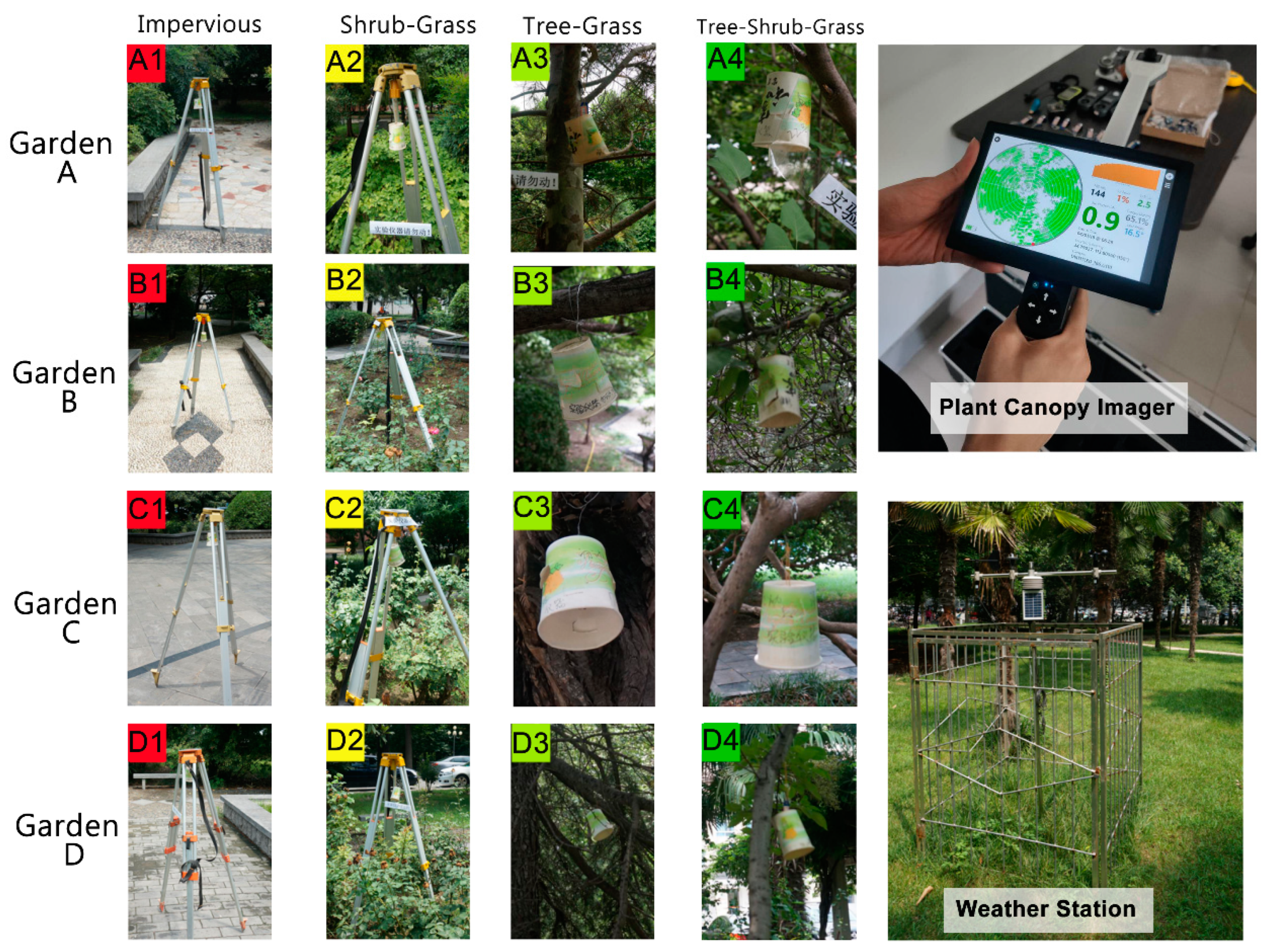
2.2. Data Measurement

This study chose four coverage types (1—impervious surface, 2—shrub–grass, 3—tree-grass, 4—tree-shrub-grass) in each garden (A, B, C, D), 16 measurement points in total (Table 1). It should be emphasized that different colors are selected according to the four types of features in the illustration. Red represents the impervious surface, yellow represents the Shrub–grass type, light green represents the Tree-grass-type, and the dark green represents the Tree-shrub-grass multilayer (≥3) community. It can be seen from the color that the richer the vegetation cover the more green it was.

2.2.1. Measurement of Air Temperature and Humidity by Using iButton

In view of the need for continuous synchronized observations at different points, 16 iButton sensors (DS 1923, Wdsen Electronic Technology Co., Ltd., Shanghai, China) were used in the study to set the same observation time and frequency. The iButton was invented and exclusively produced by Dallas Semiconductor, and can be installed almost anywhere, making it easy to use. Sensors can easily be influenced by environmental conditions [43]. In order to reduce the influence of sunlight and other factors, small radiation shields were made outside the sensor. In each site, we placed iButton sensors inside a homemade radiation shield (paper cup) at 1.5 m above the ground, the iButtons were fixed in a tripod in case of coverage type 1 and 2 (no tree cover), while the iButton in type 3 and 4 (with tree cover)were fixed in the tree directly (Figure 2).
The measurement time was conducted between 7–9 August 2019 with sunny and calm days in summer. The air temperature (AT) and relative humidity (RH) data were automatically recorded every 5 min. Considering the wind speed and direction impact on the AT and RH, the study refers to the local wind speed and wind direction (Figure 2) recorded by a long-term fixed small weather station on the campus, in order to correct and analyze the results.
Before the measurement, the 16 iButtons samples were removed from the site, shipped back to the laboratory and tested using a calibrated reference thermometer and hygrometer. The average difference between the iButton and the laboratory sensor AT was ± 0.2 °C (range 0.35 °C), and RH was ± 1.5% (range 4.5%).
The iButton and improved shielding system we used in this study had random errors, but according to the manufacturer’s specifications, the overall deviation is small. Compared with the standard research-grade sensor system, the deviation of the iButton temperature measured using a simple self-made radiation shield was <1 °C in the morning, and before sunset in the evening was <1 °C.

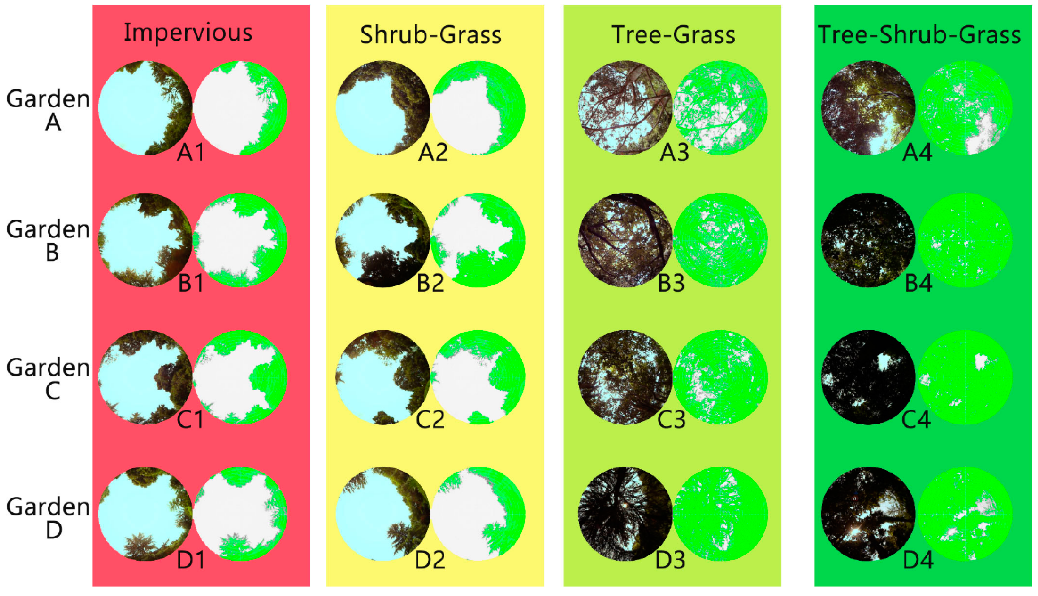
2.2.2. Measurement of Plant Canopy Parameters

In addition to temperature and humidity, we used CI-110 Plant Canopy Imager (Felix Instruments, WA, USA). The CI-110′s digital platform was enabled to simultaneously capture wide-angle plant canopy images and estimate Leaf Area Index (LAI) [44] and Photosynthetically Active Radiation (PAR) [45] levels from a single canopy scan. In order to analyze the influence of these factors on temperature and humidity, the canopy analyzer was applied to measure PAR, CD, LAI, MLA, and other data in each sample point (Table 1, Figure 3).
The units for PAR is µmol/m2s and this metric is commonly referred to as the Photosynthetic Photon Flux Density (PPFD) or the number of photons in the 400–700 nm range received by a specified area over a given period of time. This value will range from 1 µmol/m2s to 2000 µmol/m2s.
LAI is used to characterize plant and forest canopies [46]. In this study, the LAI is calculated based on the measured gap fraction of the image. This article uses the Otsu method [47,48] to calculate the LAI value of each site. The Otsu method is a commonly chosen method for mixed forest canopies. This threshold approach is a clustering-based method that classifies the threshold of an image at which intra-class variance is minimized and interclass variance is maximized. The CI-110 uses the model from John Norman [45,49] for predicting scattered and transmitted PAR and inverts it to find PAR based LAI according to the Equation below:
L =   [ ( 1 1 2 K ) f b 1 ] τ   A ( 1 0.47 f b )
where:
L = leaf area index
A = 0.283 + 0.785 a 0.159 a 2
a = leaf absorptivity in PAR wavelengths of light; this value can range from around 0.5–0.9, the CI-110 uses 0.9.
K = the extinction coefficient at each zenith angle.
f b = beam fraction
τ = ratio of below canopy PAR to above canopy PAR
The leaf angle distribution (LAD) of a plant canopy is the angular orientation of the leaves in the canopy. In LAI calculations, this is described mathematically as a statistical distribution of leaf angles on different planes. Plant canopies can range from having more erectophile leaf area distributions, such as onions which have very vertical orientation of their leaves, to more planophile, such as strawberries or oak trees that have more horizontal orientation of their leaves.

2.3. Data Analysis

Data analysis was conducted mainly from the following aspects:
  • Summarize the overall changes of the research subjects during the measurement period, comparing the effects of four types of coverage during the day and night on temperature and humidity
  • Using the measured data of different dates, analyze the spatiotemporal changes of temperature and humidity between the four types of coverage, especially the comparative analysis of the measured values of the four types of coverage, and obtain the effect of the type of coverage on the temperature and humidity changes
  • By comparing the four factors (PAR, CD, MLA and LAI) to different degrees of impact on temperature and humidity.
In the data analysis, SPSS version 25 was used to analyze and illustrate the spatiotemporal changes of temperature and humidity. At the same time, in order to compare the human comfort of different green space types, the Rayman software was used to quantify the thermal index at different points [50,51]. Specifically, Physiologically Equivalent Temperature (PET) is used as an indicator to measure human comfort. Its principle is based on human energy balance, mainly calculated from meteorological factors such as radiation intensity, air temperature, air humidity, and wind speed. The medium dressing index and human activity selection software aggregate high standard values. It should be noted that here mean radiant temperature was applied before calculating the PET, and the average radiant temperature (Tmrt) was calculated based on the method described in one article [52], and other studies have also used this method [53,54,55]. Tmrt can be regarded as the synthesis of all radiant fluxes, and it is an indicator to calculate the comprehensive influence of the surface temperature in a given area. Therefore, it is an important factor that determines human comfort, and it has better response ability in low wind and hot weather. However, the change in Tmrt depends largely on the microclimate and local factors (such as the type of surface material and coverage type), which are comprehensive factors.
We selected the noon time (11:30 a.m.–01:30 p.m.) when the radiation and the air temperature were the highest, this largely reflects the difference of vegetation types. Given the changes in weather conditions during the observation period, the median values were used in this analysis because they were a better way to generalize when outliers are present. The median value shows the midpoint of the observed value, so it is less affected by the extreme value than the average value.

3. Results

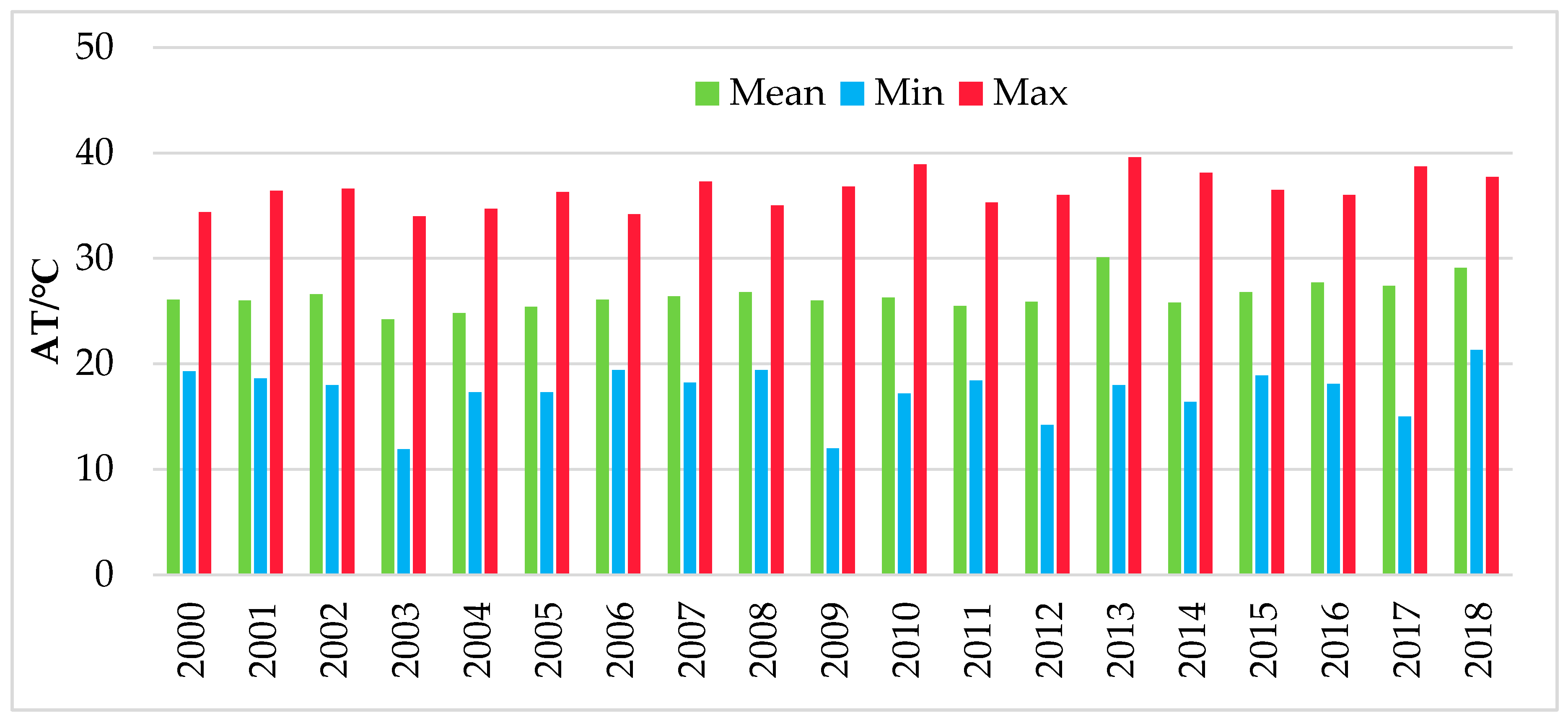
3.1. Historical Statistics of August in Zhengzhou

Based on the City Statistical Yearbook 2000–2018 [41], we extracted the long term air temperature in August of the past 18 years of Zhengzhou city (Figure 4). From the figure, the mean air temperature in August is 26.4 ℃, the minimum air temperature in August is 11.9 ℃, which appeared in the year of 2003. The maximum temperature in August in Zhengzhou was 39.6 ℃ in August 2013 is usually a hot period in summer in Zhengzhou.

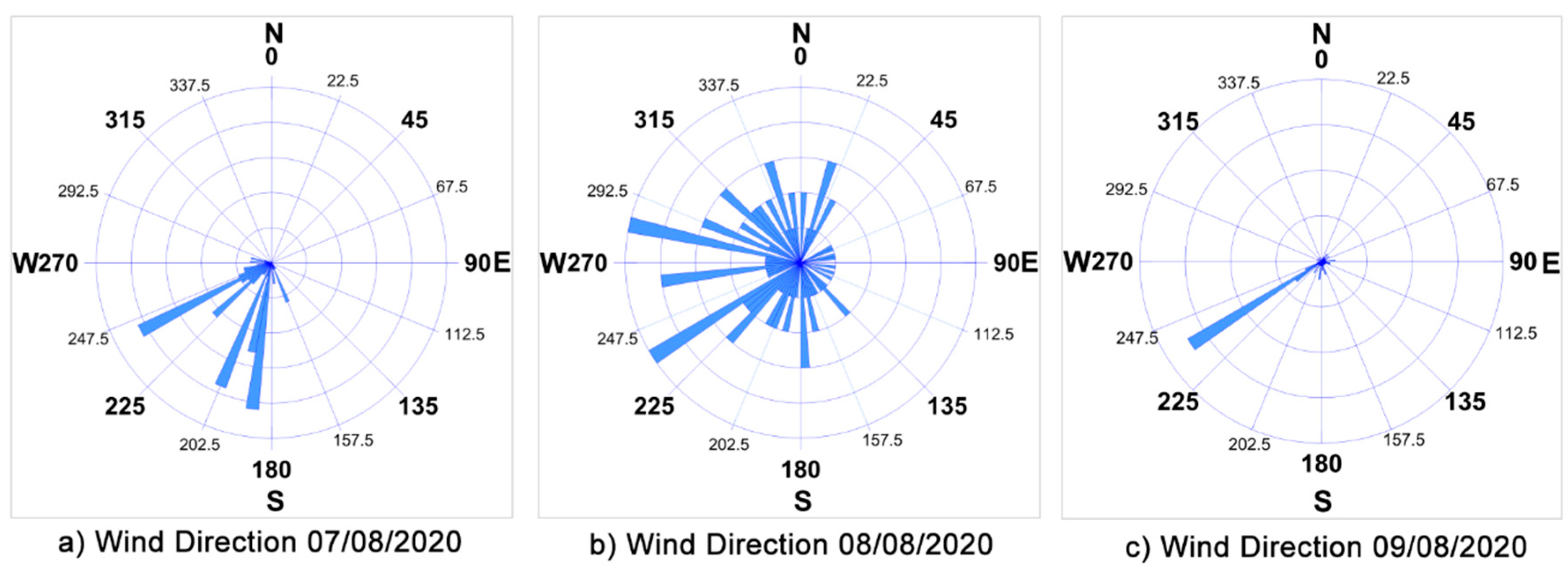
3.2. Statistical Results of Atmospheric Conditions in the Study Spots

From Table 2, the highest temperature appears in the afternoon of 8th August 2019 (01:15 p.m.), with a temperature of 40.2 °C (point A1, impervious surface). The low-temperature zone appears at midnight (11:50 p.m.), before dawn (04:15 a.m., 05:35 a.m.), the minimum temperature reaches 24.2 °C. Compared with the historical data of the same period, the value of the maximum temperature was higher than the highest value of extremely high temperatures in history. This shows that the area we studied was hotter in 2019 than the historical records of August in Zhengzhou shows. During the measurement period, the mean PET value were all above threshold 41 (Table 2), and thermal perception was “very hot”, indicating that the weather was not comfortable for human activities. People could feel extreme heat stress [50].
The median wind speed measured on the campus weather station for the three days was less than 0.1 m/s (Table 2), while the wind direction changed frequently. From compass readings in Figure 5, the wind direction was concentrated between WSW and S for the first day (07/08/2019) and was quite varied during the second day (08/08/2019), and was SW on the third day (09/08/2019) (Figure 5). However, considering the low wind speed (the average was lower than 0.1 m/s), the impact of wind on air temperature and humidity was negligible.

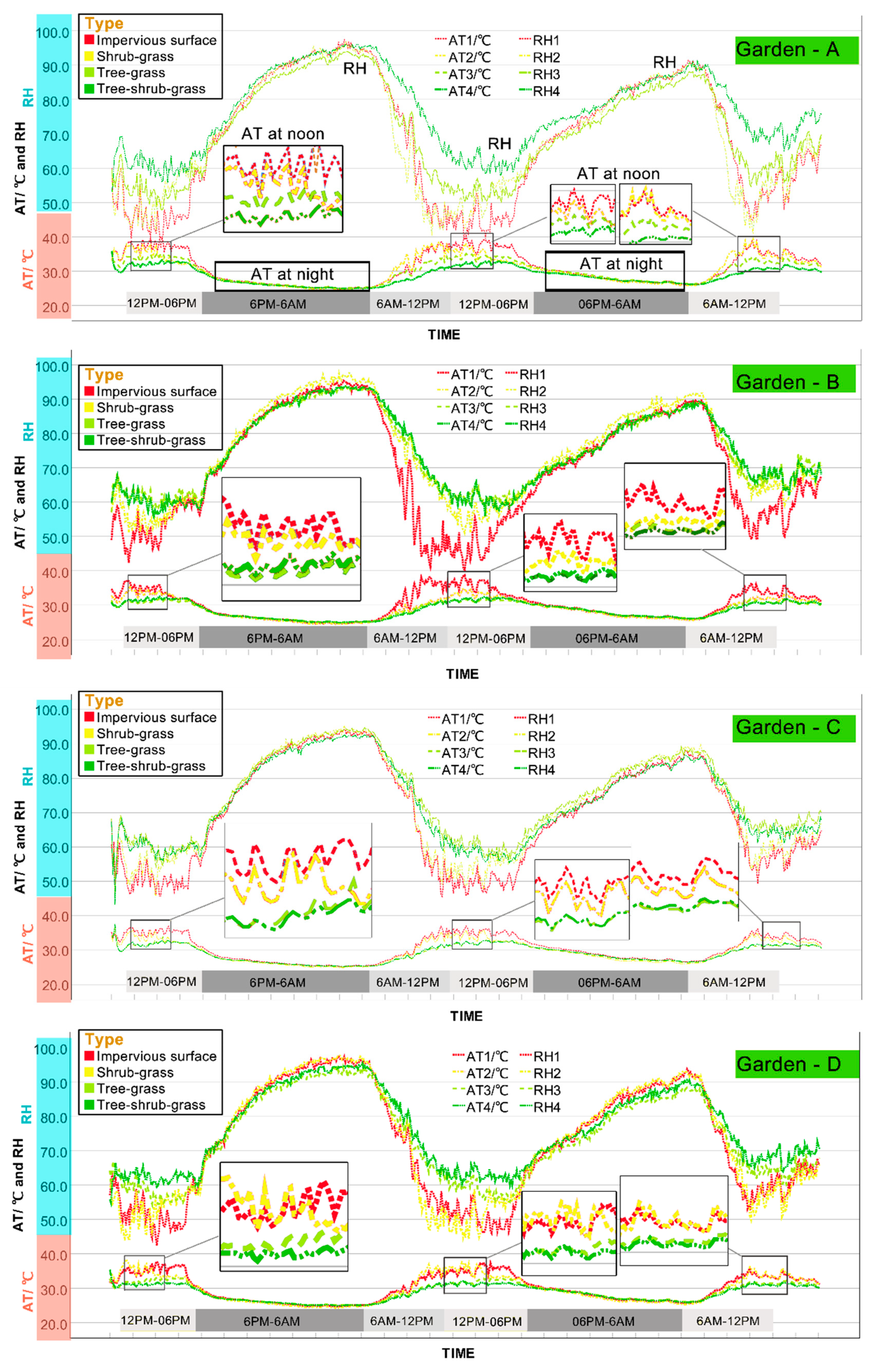
3.3. Changes in Temperature and Humidity of Different Vegetation Coverage Types

From the data (Figure 6: Garden—A, B, C and D; Coverage type 1, 2, 3 and 4), the following results can be obtained:
(1)
The air temperature shows as type 1> type 2> type 3> type 4, but the humidity was opposite, indicating that more vegetation coverage makes the temperature lower and makes the surrounding more humid.
(2)
The difference between the four coverage types was not the same during the day and night in temperature and humidity. The difference in the morning (around 6:00 a.m.) and evening (06:00 p.m.) was smaller than that of around noon, because the four types differ significantly in temperature and humidity values around noon. At night (06:00 p.m.–6:00 a.m.), the temperature and humidity values of four coverage types were relatively close. It is worth noting that the humidity of the impervious surface was greater at night, sometimes higher than the humidity of the other three vegetation coverage types, but with relatively close temperature values.
(3)
The four coverage types (1, 2, 3 and 4) essentially showed the same symptom (Figure 6). The type 1 (impervious surface) had the highest temperature and the lowest relative humidity, but the type 4 (tree-shrub-grass) multilayer vegetation structure has the lowest temperature. The maximum temperature difference could reach 8.9 ℃ (Garden B: B1 and B4, 09/08/2019, 10:45 a.m.). The maximum relative humidity difference was 28.5% (Garden B: B1 and B4). Even the lowest temperature difference reached 5.2 ℃ (Garden C, C1 and C4, 08/08/2019, 11:34 a.m.), and the humidity difference was 14.4% (Garden C: C1 and C4, 08/08/2019, 11:25 a.m.). At noon, the temperature of type 2 (shrub-grass) and type 1 was significantly higher than the type 3 (tree-grass) and type 4, indicating that the tree cover was the core factor affecting temperature, but from the comparison of humidity. The humidity of type 3 and type 4 was much higher than that of type 1 and type 2, indicating that tree cover could increase the humidity of the environment.

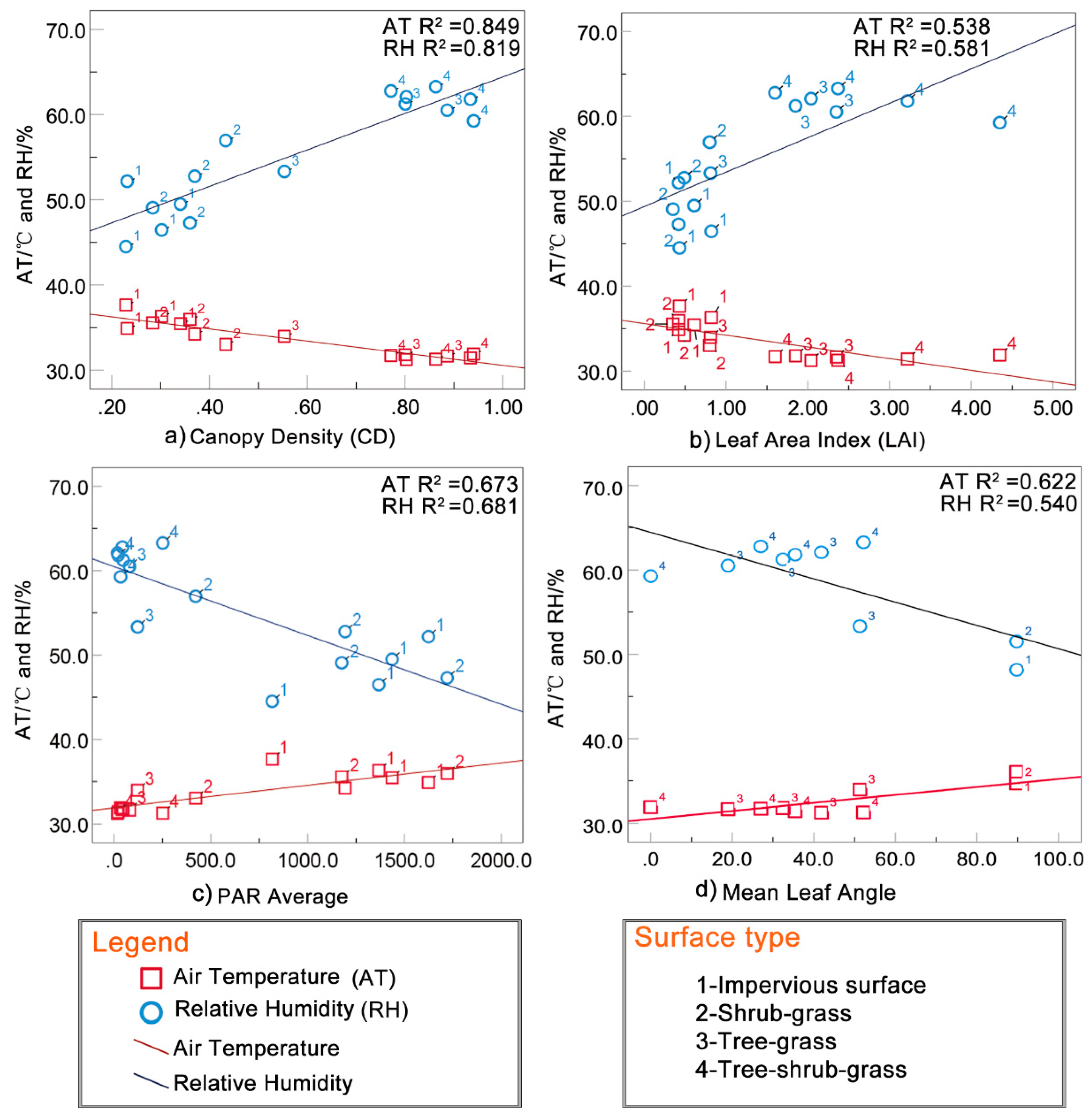
3.4. Comparison of Influencing Factors

Around noon (11:30 a.m.–12:30 p.m.), solar radiation was the largest. Vegetation coverage, shadows and photosynthesis have the strongest influence on the surface. From Figure 7, the canopy density (CD), leaf area index (LAI), photosynthetically active radiation (PAR), mean leaf angle (MLA) had an effect on air temperature and relative humidity. First, Pearson correlation was used to analyze the influencing factors. The results showed that the correlation between air temperature (AT) and relative humidity (RH) and plant community characteristics was very high (both were greater than 0.7, p < 0.001). The highest correlation between RH and CD reached 0.921 (negative correlation) and 0.905 (positive correlation), respectively (Table 3). In short, there was a close correlation between temperature, relative humidity, surface cover types and vegetation structural characteristics (Figure 7). Further analysis was therefore required to understand the regression relationship between the characteristics of vegetation structure and the effect of cooling and humidification.
The results of linear regression analysis revealed that CD (R2AT = 0.848, R2RH = 0.819, respectively, Figure 8a) and LAI (R2AT = 0.538, R2RH = 0.581, respectively, Figure 8b) had a positive effect on cooling air temperature and increasing relative humidity, while average PAR and MLA had a negative effect on cooling AT and increasing RH (Figure 8c,d). In relation to the vegetation characteristics (CD and LAI), the CD on cooling and humidification was more significant than that of LAI. In addition, it was discovered that other factors such as solar radiation and wind speed also could affect cooling and humidification effects [56,57]. The regression results showed that solar radiation had a positive significant effect on increasing temperature and decreasing relative humidity (Table 3, Figure 7 and Figure 8c). However, due to the small range of changes in wind speed during the observation period (Table 2), its impact on temperature and relative humidity was small, thus, no separate analysis was performed.

4. Discussion

4.1. Influence of Coverage Types on Thermal Microclimate

Previous studies on urban heat islands on a large scale indicated that the heat island intensity during the day changed differently from the heat islands at night, and the UHI intensity at night was greater [10,58]. However, on a small scale, as observed in this study, the temperature difference between the vegetation space and the non-vegetation space was small at night, but the air temperature and relative humidity difference during the day were large. Thus, we can realize that SGS has faster heat conduction with the surrounding than that between urban and rural regions. The cooling effect of green space can be explained essentially from the perspective of heat balance [59]. First of all, the heat source comes from solar radiation. Infrared rays in sunlight can warm up the irradiated material, and the temperature of the material is mainly determined by the heat capacity of the material itself. Compared with the impervious surface, the leaves of plants have higher heat capacity. Therefore, under the same amount of radiation and time, the temperature of the area covered by the plant rises more slowly, mainly due to photosynthesis. In this process, the evaporation of water from the earth will evaporate the heat and reduce the temperature. Secondly, we can also use the Bowen ratio to explain some of the results in this article. The Bowen ratio is the ratio of sensible heat flux to latent heat flux [60,61]. In heat conduction, the heat energy (sensible heat flux) absorbed by the green space from the surrounding environment should be equal to the excess energy resistance (latent heat flux) generated by photosynthesis and transpiration, to balance the heat conduction. More green space means more energy dissipation, which leads to more heat energy conduction. Therefore, the types with high vegetation cover density and larger plant leaf area density have higher energy resistance, thereby reducing the Bowen ratio, and the cooling effect is also the most significant.
The cooling effect of different coverage types can also be explained by surface “radiative properties” such as albedo and emissivity [62,63]. The solar reflectance or albedo is the percentage of solar energy reflected by a surface. At noon, the radiation was the highest period, as for impervious surface type, which had a lower albedo than that of vegetation coverage types (2—Shrub-grass; 3—Tree-grass; 4—Tree-shrub-grass in this article) in this study. Generally, an impervious surface reflects less and absorbs more of the sun’s energy. Therefore, this type (no vegetation cover) has a higher temperature than the other three types (cover with vegetation).
The impervious surface is the core area of the urban heat island. In agreement with the large-scale research [16,64,65], among the different types of urban land use, the UHI is mainly concentrated in the urban impervious areas, such as industrial areas, urban squares, roads, building roofs, and other gray infrastructure. The urban cold islands (UCI) are mainly concentrated in urban green space (UGS) and water areas such as urban forests, parks and water systems. The city is an enlarged version of gardens, including impervious surface and vegetated surface, as an analogy to some extent. The different cover types of SGS also reflect the different spatial distribution of the city and the UHI phenomena is quite similar.

4.2. Influence of Vegetation Structure on Microclimate

Concerning the characteristics of plant communities, this study showed that trees are the key factors affecting the canopy layer urban heat island effect and comfort. The same results are shown in previous studies [66,67,68]. The cooling effect is related to tree shade, building shading, and other shadows, which reduce radiation and lower temperature [25,57,63,69]. Compared with building shadows, plants not only provide shade, but also increase humidity [57,70]. Other studies had also drawn relevant conclusions; in Zhengzhou city (China), large parks have a significant cooling effect, and the cooling effect is positively related to the vegetation coverage inside of the park [29,71]. In the urban parks of Taipei, the average PCI during the daytime in summer is only 0.81 ℃ but no consistent cooling effect was found in small parks (less than three hectares). The low cooling effect of these green spaces is probably related to high humidity levels, and consequently, low evapotranspiration [30]. In the study of parks in Lisbon (Portugal), the maximum cooling temperature of the city park reached 6.9 ℃, and the cooling temperature was related to the shadow of the building and the surrounding shape [72]. In an Algerian microclimate study, the vegetation could produce an average cooling effect of 2℃ to 3 ℃. The calculation showed that the maximum cooling range at night could reach 10 ℃ [32]. In Nagoya (Japan), it was found that the temperature difference between the studied green area and the surrounding was low, but this cooling effect was found to last for hundreds of meters or more [73]. In view of the above results, it is necessary to conduct localization studies for each urban environment in order to adapt and to maximize the benefits of green spaces based on the characteristics of each city.
In previous studies, the entire plant community was different at different times and in different seasons, but they all had significant cooling and humidifying effects throughout the year (four seasons) [73,74]. In the case of human comfort, vegetation has the greatest cooling and humidification effect in summer. This further supports the conclusion that the higher the temperature, the stronger the cooling effect of vegetation [75]. In this study, the maximum temperature difference between multi-layer vegetation communities and the impervious surface ranged from 5.2 ℃ to 8.9 ℃, and the maximum relative humidity difference ranged from 14.4% to 28.5%.
We found that multi-layer plant communities were most effective in cooling and humidifying effects, but the plant community was diverse in structure and rich in variety. In addition, the leaf area of the multi-layer plant communities was larger than other coverage types. Vegetation communities (with tree coverage) can reflect more direct solar radiation than other vegetation communities (no-tree cover) [76,77]. This study also proved that the cooling and humidifying effects of shrubs and grass plant communities were significantly lower than those of canopy-covered tree communities. This study identified four factors that affect temperature and relative humidity. The regression results on the factors that affect the cooling and humidifying effect showed that the four factors of CD, LAI, MLA and PAR had a significant effect on the cooling and relative humidity increase. CD was the most effective for cooling and humidification. In addition, under the same type of multi-layer plant community structure, the angle of the leaves also influences the cooling effect. Specifically, the smaller the angle between the plant leaf and the horizontal plane, the more evident the effect of cooling and humidification. These findings can provide a basis and reference for landscape architects. However, other elements (such as tree shape, evapotranspiration, plant age) need further study to understand the quantitative relationship of plant communities.

4.3. Implications for Urban Planning and Landscape Design

Under the urban homogenization hypothesis [35,36,37], urban design is becoming more and more homogenous. The ecological functions of plant communities are similar. They all have evident cooling and humidifying effects on the urban microclimate. The microclimate and heat island regulation function of SGS and their role in urban comfort cannot be ignored. SGSs are more conducive to renovation and renewal than large green spaces to some extent. The results of this study may help future urban design and urban renewal. In summary, this study makes the following recommendations:
  • It is recommended that urban planners increase the number and proportion of green spaces in the city and increase the tree canopy coverage in the overall urban planning process.
  • In city planning, plant species design should be based on the local climatic conditions, increasing the multi-layered community structure of the plant, considering the characteristics of the leaf area index and the blade angle of the plant.
  • In a small-scale green space landscape design, conifers should be combined with broad-leaved trees, and the tree-shrub-grass compound should be designed to maximize the cooling and humidification effects of the microclimate.

5. Conclusions

The research results in this paper provide a scientific basis for characterizing the microclimate changes of green space. In this study, the field observation and measurement method was used to study the relationship between temperature and humidity among types of small green space (SGS). By selecting four green spaces in the university campus as sample spots, using meteorological data to analyze spatial and temporal characteristics of the SGSs, we compared the effects of four coverage types (1—impervious surface; 2—shrub-grass; 3—tree-grass; 4—tree-shrub-grass) on microclimate. Finally, we analyzed the four impact factors (PAR, CD, MLA, LAI) of the SGSs among all 16 spots. The research results in this paper provide a scientific basis for characterizing the microclimate of green space. The conclusions of this article were as follows:
  • There were evident differences in temperature between the four types in SGSs. The largest difference was concentrated in the noon period when solar radiation was strongest during the day, but the difference between the types at night was small. Specifically, the difference in temperature and humidity between the four types during the day was large, and the temperature was expressed as AT1 > AT2 > AT3 > AT4. At noon, the difference reached the maximum, and the relative humidity order was the opposite RH4 > RH3 > RH2 > RH1. The four coverage types showed that the temperature and humidity values were relatively close at night.
  • The four coverage types of four gardens essentially showed the same trend. Type 1 (impervious surface) had the highest temperature and the lowest relative humidity, while the type 4 (tree-shrub-grass) multi-layer vegetation structure had the lowest temperature and the highest humidity. This type had the highest temperature difference as well, that can reach 8.9 ℃ (Garden B, B1, and B4, 09/08/2019, 10:45 a.m.). The maximum relative humidity difference was 28.5% (Garden B, B1 and B4). Those results showed that tree cover types were cooler and more humid than no tree-cover types, which reveals that tree cover was the core factor affecting the temperature.
  • There was a close correlation between surface coverage types and plant community characteristics. Canopy density (CD) and leaf area index (LAI) had a positive effect on cooling and relative humidity, while photosynthetically active radiation (PAR) and mean leaf angle (MLA) had a negative effect on cooling and relative humidity.
In order to better understand all the factors that explain the impact of green areas in their surrounding environment, further research is needed to take into account the specific characteristics of urban green space. The results can provide recommendations for green space management and future landscape design, which can alleviate urban heat island effects, and enhance and improve the ecological benefits of urban green spaces.

Author Contributions

Conceptualization, H.L., H.M. and S.J.; methodology, H.L.; investigation, Y.G., R.H.; software, H.L., R.H.; resources, G.T. and Y.L.; writing—original draft preparation, H.L. and H.M.; writing—review and editing, H.L. and S.J. visualization, S.J. and A.-a.E. All authors have read and agreed to the published version of the manuscript.

Funding

This research was funded by “Henan Province Young Talent Support Project (2019HYTP033), Henan Meteorological Science and Technology Research Project (KM201809, KM201810) and “Henan Overseas Expertise Introduction Center for Discipline Innovation”.

Acknowledgments

First: we would thank the Stipendium Hungaricum Programme funding for supporting our research. Second, we would also thank our team colleagues in Henan Agricultural University; and the colleagues in the Department of Planning and Regional Development in Szent István University as well. In addition, we would also like to thank the referees and the editors for their valuable comments for improving this manuscript.

Conflicts of Interest

The authors declare no conflict of interest.

References

  1. United Nations. World Population Prospects 2019–Volume II: Demographic Profiles; UN: New York, NY, USA, 2020; ISBN 978-92-1-004643-5. [Google Scholar]
  2. United Nations; Department of Economic and Social Affairs; Population Division. World Urbanization Prospects: The 2018 Revision; UN: New York, NY, USA, 2019; ISBN 978-92-1-148319-2. [Google Scholar]
  3. Bottema, M. Urban roughness modelling in relation to pollutant dispersion. Atmos. Environ. 1997, 31, 3059–3075. [Google Scholar] [CrossRef]
  4. Rodler, A.; Leduc, T. Local climate zone approach on local and micro scales: Dividing the urban open space. Urban Clim. 2019, 28, 100457. [Google Scholar] [CrossRef]
  5. Alexander, P.J.; Fealy, R.; Mills, G.M. Simulating the impact of urban development pathways on the local climate: A scenario-based analysis in the greater Dublin region, Ireland. Landsc. Urban Plan. 2016, 152, 72–89. [Google Scholar] [CrossRef] [Green Version]
  6. Reichle, D.E. Chapter 11—Anthropogenic alterations to the global carbon cycle and climate change. In The Global Carbon Cycle and Climate Change; Reichle, D.E., Ed.; Elsevier: Amsterdam, The Netherlands, 2020; pp. 209–251. ISBN 978-0-12-820244-9. [Google Scholar]
  7. Thani, S.K.S.O.; Mohamad, N.H.N.; Abdullah, S.M.S. The Influence of Urban Landscape Morphology on the Temperature Distribution of Hot-Humid Urban Centre. Procedia Soc. Behav. Sci. 2013, 85, 356–367. [Google Scholar] [CrossRef] [Green Version]
  8. Ng, E.; Yuan, C.; Chen, L.; Ren, C.; Fung, J.C.H. Improving the wind environment in high-density cities by understanding urban morphology and surface roughness: A study in Hong Kong. Landsc. Urban Plan. 2011, 101, 59–74. [Google Scholar] [CrossRef]
  9. Howard, L. The Climate of London: Deduced from Meteorological Observations, Made at Different Places in the Neighbourhood of the Metropolis; Phillips, W., Ed.; George Yard: San Francisco, CA, USA, 1818. [Google Scholar]
  10. Oke, T.R. The energetic basis of the urban heat island. Q. J. R. Meteorol. Soc. 1982, 108, 1–24. [Google Scholar] [CrossRef]
  11. Jenerette, G.D.; Harlan, S.L.; Brazel, A.; Jones, N.; Larsen, L.; Stefanov, W.L. Regional relationships between surface temperature, vegetation, and human settlement in a rapidly urbanizing ecosystem. Landsc. Ecol. 2007, 22, 353–365. [Google Scholar] [CrossRef]
  12. Jiang, J.; Tian, G. Analysis of the impact of Land use/Land cover change on Land Surface Temperature with Remote Sensing. Procedia Environ. Sci. 2010, 2, 571–575. [Google Scholar] [CrossRef] [Green Version]
  13. Jiménez-Muñoz, J.C.; Sobrino, J.A.; Skoković, D.; Mattar, C.; Cristóbal, J. Land Surface Temperature Retrieval Methods from Landsat-8 Thermal Infrared Sensor Data. IEEE Geosci. Remote Sens. Lett. 2014, 11, 1840–1843. [Google Scholar] [CrossRef]
  14. Tomlinson, C.J.; Chapman, L.; Thornes, J.E.; Baker, C. Remote sensing land surface temperature for meteorology and climatology: A review: Remote sensing land surface temperature. Meteorol. Appl. 2011, 18, 296–306. [Google Scholar] [CrossRef] [Green Version]
  15. Bokaie, M.; Zarkesh, M.K.; Arasteh, P.D.; Hosseini, A. Assessment of Urban Heat Island based on the relationship between land surface temperature and Land Use/Land Cover in Tehran. Sustain. Cities Soc. 2016, 23, 94–104. [Google Scholar] [CrossRef]
  16. Azhdari, A.; Soltani, A.; Alidadi, M. Urban morphology and landscape structure effect on land surface temperature: Evidence from Shiraz, a semi-arid city. Sustain. Cities Soc. 2018, 41, 853–864. [Google Scholar] [CrossRef]
  17. Antoniadis, D.; Katsoulas, N.; Kittas, C. Simulation of schoolyard’s microclimate and human thermal comfort under Mediterranean climate conditions: Effects of trees and green structures. Int. J. Biometeorol. 2018, 62, 2025–2036. [Google Scholar] [CrossRef] [PubMed]
  18. Galagoda, R.U.; Jayasinghe, G.Y.; Halwatura, R.U.; Rupasinghe, H.T. The impact of urban green infrastructure as a sustainable approach towards tropical micro-climatic changes and human thermal comfort. Urban For. Urban Green. 2018, 34, 1–9. [Google Scholar] [CrossRef]
  19. Mao, J.; Yang, J.H.; Afshari, A.; Norford, L.K. Global sensitivity analysis of an urban microclimate system under uncertainty: Design and case study. Build. Environ. 2017, 124, 153–170. [Google Scholar] [CrossRef]
  20. Adelia, A.S.; Yuan, C.; Liu, L.; Shan, R.Q. Effects of urban morphology on anthropogenic heat dispersion in tropical high-density residential areas. Energy Build. 2019, 186, 368–383. [Google Scholar] [CrossRef]
  21. Salvati, A.; Palme, M.; Chiesa, G.; Kolokotroni, M. Built form, urban climate and building energy modelling: Case-studies in Rome and Antofagasta. J. Build. Perform. Simul. 2020, 13, 209–225. [Google Scholar] [CrossRef]
  22. Lin, W.; Yu, T.; Chang, X.; Wu, W.; Zhang, Y. Calculating cooling extents of green parks using remote sensing: Method and test. Landsc. Urban Plan. 2015, 134, 66–75. [Google Scholar] [CrossRef]
  23. Zardo, L.; Geneletti, D.; Pérez-Soba, M.; Van Eupen, M. Estimating the cooling capacity of green infrastructures to support urban planning. Ecosyst. Serv. 2017, 26, 225–235. [Google Scholar] [CrossRef]
  24. Kotthaus, S.; Grimmond, C.S.B. Energy exchange in a dense urban environment—Part I: Temporal variability of long-term observations in central London. Urban Clim. 2014, 10, 261–280. [Google Scholar] [CrossRef] [Green Version]
  25. Andreou, E. The effect of urban layout, street geometry and orientation on shading conditions in urban canyons in the Mediterranean. Renew. Energy 2014, 63, 587–596. [Google Scholar] [CrossRef]
  26. Skelhorn, C.; Lindley, S.; Levermore, G. The impact of vegetation types on air and surface temperatures in a temperate city: A fine scale assessment in Manchester, UK. Landsc. Urban Plan. 2014, 121, 129–140. [Google Scholar] [CrossRef]
  27. Du, H.; Song, X.; Jiang, H.; Kan, Z.; Wang, Z.; Cai, Y. Research on the cooling island effects of water body: A case study of Shanghai, China. Ecol. Indic. 2016, 67, 31–38. [Google Scholar] [CrossRef]
  28. Hamada, S.; Tanaka, T.; Ohta, T. Impacts of land use and topography on the cooling effect of green areas on surrounding urban areas. Urban For. Urban Green. 2013, 12, 426–434. [Google Scholar] [CrossRef]
  29. Li, H.; Wang, G.; Tian, G.; Jombach, S. Mapping and Analyzing the Park Cooling Effect on Urban Heat Island in an Expanding City: A Case Study in Zhengzhou City, China. Land 2020, 9, 57. [Google Scholar] [CrossRef] [Green Version]
  30. Cao, X.; Onishi, A.; Chen, J.; Imura, H. Quantifying the cool island intensity of urban parks using ASTER and IKONOS data. Landsc. Urban Plan. 2010, 96, 224–231. [Google Scholar] [CrossRef]
  31. Du, H.; Cai, W.; Xu, Y.; Wang, Z.; Wang, Y.; Cai, Y. Quantifying the cool island effects of urban green spaces using remote sensing Data. Urban For. Urban Green. 2017, 27, 24–31. [Google Scholar] [CrossRef]
  32. Bencheikh, H.; Rchid, A. The Effects of Green Spaces (Palme Trees) on the Microclimate in Arides Zones, Case Study: Ghardaia, Algeria. Energy Procedia 2012, 18, 10–20. [Google Scholar] [CrossRef] [Green Version]
  33. Wang, Y.; Bakker, F.; de Groot, R.; Wörtche, H. Effects of urban green infrastructure (UGI) on local outdoor microclimate during the growing season. Environ. Monit. Assess. 2015, 187. [Google Scholar] [CrossRef] [Green Version]
  34. Park, J.; Kim, J.-H.; Lee, D.K.; Park, C.Y.; Jeong, S.G. The influence of small green space type and structure at the street level on urban heat island mitigation. Urban For. Urban Green. 2017, 21, 203–212. [Google Scholar] [CrossRef]
  35. Lososová, Z.; Chytrý, M.; Tichý, L.; Danihelka, J.; Fajmon, K.; Hájek, O.; Kintrová, K.; Láníková, D.; Otýpková, Z.; Řehořek, V. Biotic homogenization of Central European urban floras depends on residence time of alien species and habitat types. Biol. Conserv. 2012, 145, 179–184. [Google Scholar] [CrossRef]
  36. Groffman, P.M.; Cavender-Bares, J.; Bettez, N.D.; Grove, J.M.; Hall, S.J.; Heffernan, J.B.; Hobbie, S.E.; Larson, K.L.; Morse, J.L.; Neill, C.; et al. Ecological homogenization of urban USA. Front. Ecol. Environ. 2014, 12, 74–81. [Google Scholar] [CrossRef] [Green Version]
  37. Pearse, W.D.; Cavender-Bares, J.; Hobbie, S.E.; Avolio, M.L.; Bettez, N.; Chowdhury, R.R.; Darling, L.E.; Groffman, P.M.; Grove, J.M.; Hall, S.J.; et al. Homogenization of plant diversity, composition, and structure in North American urban yards. Ecosphere 2018, 9, 1–17. [Google Scholar] [CrossRef]
  38. Yang, J.; Yan, P.; Li, X. Urban biodiversity in China: Who are winners? Who are losers? Sci. Bull. 2016, 61, 1631–1633. [Google Scholar] [CrossRef] [Green Version]
  39. Qian, S.; Qi, M.; Huang, L.; Zhao, L.; Lin, D.; Yang, Y. Biotic homogenization of China’s urban greening: A meta-analysis on woody species. Urban For. Urban Green. 2016, 18, 25–33. [Google Scholar] [CrossRef]
  40. Rasul, A.; Balzter, H.; Smith, C.; Remedios, J.; Adamu, B.; Sobrino, J.; Srivanit, M.; Weng, Q. A Review on Remote Sensing of Urban Heat and Cool Islands. Land 2017, 6, 38. [Google Scholar] [CrossRef] [Green Version]
  41. Zhengzhou Municipal Bureau of Statistics. Zheng Zhou Statistical Yearbook 2018; China Statistics Press: Beijing, China, 2018; ISBN 978-7-5037-8600-6. [Google Scholar]
  42. Beck, H.E.; Zimmermann, N.E.; McVicar, T.R.; Vergopolan, N.; Berg, A.; Wood, E.F. Present and future Köppen-Geiger climate classification maps at 1-km resolution. Sci. Data 2018, 5, 180214. [Google Scholar] [CrossRef] [Green Version]
  43. Zaukuu, J.L.Z.; Bazar, G.; Gillay, Z.; Kovacs, Z. Emerging trends of advanced sensor based instruments for meat, poultry and fish quality—A review. Crit. Rev. Food Sci. Nutr. 2019, 1–18. [Google Scholar] [CrossRef]
  44. Vanderbilt, V.C. Measuring plant canopy structure. Remote Sens. Environ. 1985, 18, 281–294. [Google Scholar] [CrossRef]
  45. Norman, J.M.; Jarvis, P.G. Photosynthesis in Sitka Spruce (Picea sitchensis (Bong.) Carr.). III. Measurements of Canopy Structure and Interception of Radiation. J. Appl. Ecol. 1974, 11, 375–398. [Google Scholar] [CrossRef]
  46. Carlson, T.N.; Ripley, D.A. On the relation between NDVI, fractional vegetation cover, and leaf area index. Remote Sens. Environ. 1997, 62, 241–252. [Google Scholar] [CrossRef]
  47. Sezgin, M.; Sankur, B. Survey over image thresholding techniques and quantitative performance evaluation. J. Eelectron. Imaging 2004, 13, 146–165. [Google Scholar] [CrossRef]
  48. Otsu, N. A Threshold Selection Method from Gray-Level Histograms. IEEE Trans. Syst. ManCybern. 1979, 9, 62–66. [Google Scholar] [CrossRef] [Green Version]
  49. Norman, J.M.; Campbell, G.S. Canopy structure. In Plant Physiological Ecology: Field Methods and Instrumentation; Pearcy, R.W., Ehleringer, J.R., Mooney, H.A., Rundel, P.W., Eds.; Springer: Dordrecht, The Netherlands, 1989; pp. 301–325. ISBN 978-94-009-2221-1. [Google Scholar]
  50. Sharmin, T.; Steemers, K.; Humphreys, M. Outdoor thermal comfort and summer PET range: A field study in tropical city Dhaka. Energy Build. 2019, 198, 149–159. [Google Scholar] [CrossRef]
  51. Oh, W.; Ooka, R.; Nakano, J.; Kikumoto, H.; Ogawa, O. Evaluation of mist-spraying environment on thermal sensations, thermal environment, and skin temperature under different operation modes. Build. Environ. 2020, 168, 106484. [Google Scholar] [CrossRef]
  52. Jendritzky, G.; Nübler, W. A model analysing the urban thermal environment in physiologically significant terms. Arch. Met. Geoph. Biocl. Ser. B 1981, 29, 313–326. [Google Scholar] [CrossRef]
  53. Thorsson, S.; Lindberg, F.; Eliasson, I.; Holmer, B. Different methods for estimating the mean radiant temperature in an outdoor urban setting. Int. J. Climatol. 2007, 27, 1983–1993. [Google Scholar] [CrossRef]
  54. Lee, H.; Mayer, H. Validation of the mean radiant temperature simulated by the RayMan software in urban environments. Int. J. Biometeorol. 2016, 60, 1775–1785. [Google Scholar] [CrossRef]
  55. Cohen, S.; Palatchi, Y.; Palatchi, D.P.; Shashua-Bar, L.; Lukyanov, V.; Yaakov, Y.; Matzarakis, A.; Tanny, J.; Potchter, O. Mean radiant temperature in urban canyons from solar calculations, climate and surface properties—Theory, validation and ‘Mr.T’ software. Build. Environ. 2020, 178, 106927. [Google Scholar] [CrossRef]
  56. Shashua-Bar, L.; Pearlmutter, D.; Erell, E. The cooling efficiency of urban landscape strategies in a hot dry climate. Landsc. Urban Plan. 2009, 92, 179–186. [Google Scholar] [CrossRef]
  57. Lin, B.-S.; Lin, Y.-J. Cooling Effect of Shade Trees with Different Characteristics in a Subtropical Urban Park. HortScience 2010, 45, 83–86. [Google Scholar] [CrossRef] [Green Version]
  58. US EPA. Heat Island Effect. Available online: https://www.epa.gov/heat-islands (accessed on 17 October 2018).
  59. Monteith, J.L.; Unsworth, M.H. Principles of Environmental Physics: Plants, Animals, and the Atmosphere, 4th ed.; Elsevier: Amsterdam, The Netherlands; Academic Press: Boston, MA, USA, 2013; ISBN 978-0-12-386910-4. [Google Scholar]
  60. Bowen, I.S. The Ratio of Heat Losses by Conduction and by Evaporation from any Water Surface. Phys. Rev. 1926, 27, 779–787. [Google Scholar] [CrossRef] [Green Version]
  61. Kanda, M.; Moriizumi, T. Momentum and Heat Transfer over Urban-like Surfaces. Bound. Layer Meteorol. 2009, 131, 385–401. [Google Scholar] [CrossRef]
  62. Bhattacharya, B.K.; Mallick, K.; Padmanabhan, N.; Patel, N.K.; Parihar, J.S. Retrieval of land surface albedo and temperature using data from the Indian geostationary satellite: A case study for the winter months. Int. J. Remote Sens. 2009, 30, 3239–3257. [Google Scholar] [CrossRef]
  63. Erell, E.; Pearlmutter, D.; Boneh, D.; Kutiel, P.B. Effect of high-albedo materials on pedestrian heat stress in urban street canyons. Urban Clim. 2014, 10, 367–386. [Google Scholar] [CrossRef]
  64. Doick, K.J.; Peace, A.; Hutchings, T.R. The role of one large greenspace in mitigating London’s nocturnal urban heat island. Sci. Total Environ. 2014, 493, 662–671. [Google Scholar] [CrossRef]
  65. Li, Y.; Zhang, H.; Kainz, W. Monitoring patterns of urban heat islands of the fast-growing Shanghai metropolis, China: Using time-series of Landsat TM/ETM+ data. Int. J. Appl. Earth Obs. Geoinf. 2012, 19, 127–138. [Google Scholar] [CrossRef]
  66. Taleghani, M.; Kleerekoper, L.; Tenpierik, M.; van den Dobbelsteen, A. Outdoor thermal comfort within five different urban forms in the Netherlands. Build. Environ. 2015, 83, 65–78. [Google Scholar] [CrossRef]
  67. Jamei, E.; Rajagopalan, P.; Seyedmahmoudian, M.; Jamei, Y. Review on the impact of urban geometry and pedestrian level greening on outdoor thermal comfort. Renew. Sustain. Energy Rev. 2016, 54, 1002–1017. [Google Scholar] [CrossRef]
  68. Yan, H.; Wu, F.; Dong, L. Influence of a large urban park on the local urban thermal environment. Sci. Total Environ. 2018, 622–623, 882–891. [Google Scholar] [CrossRef]
  69. Chen, J.; Jin, S.; Du, P. Roles of horizontal and vertical tree canopy structure in mitigating daytime and nighttime urban heat island effects. Int. J. Appl. Earth Obs. Geoinf. 2020, 89, 102060. [Google Scholar] [CrossRef]
  70. Armson, D.; Stringer, P.; Ennos, A.R. The effect of tree shade and grass on surface and globe temperatures in an urban area. Urban For. Urban Green. 2012, 11, 245–255. [Google Scholar] [CrossRef]
  71. Li, H.; Wang, G.; Tian, G.; Jombach, S. Mapping and Assessment of the Urban Heat Island in Zhengzhou City. Proc. Fábos Conf. Landsc. Greenway Plan. 2019, 6, 38. [Google Scholar] [CrossRef]
  72. Oliveira, S.; Andrade, H.; Vaz, T. The cooling effect of green spaces as a contribution to the mitigation of urban heat: A case study in Lisbon. Build. Environ. 2011, 46, 2186–2194. [Google Scholar] [CrossRef]
  73. Hamada, S.; Ohta, T. Seasonal variations in the cooling effect of urban green areas on surrounding urban areas. Urban For. Urban Green. 2010, 9, 15–24. [Google Scholar] [CrossRef]
  74. Mathew, A.; Khandelwal, S.; Kaul, N. Investigating spatial and seasonal variations of urban heat island effect over Jaipur city and its relationship with vegetation, urbanization and elevation parameters. Sustain. Cities Soc. 2017, 35, 157–177. [Google Scholar] [CrossRef]
  75. Shi, D.; Song, J.; Huang, J.; Zhuang, C.; Guo, R.; Gao, Y. Synergistic cooling effects (SCEs) of urban green-blue spaces on local thermal environment: A case study in Chongqing, China. Sustain. Cities Soc. 2020, 55, 102065. [Google Scholar] [CrossRef]
  76. Wang, Y.; Akbari, H. The effects of street tree planting on Urban Heat Island mitigation in Montreal. Sustain. Cities Soc. 2016, 27, 122–128. [Google Scholar] [CrossRef]
  77. Yang, W.; Lin, Y.; Li, C.-Q. Effects of Landscape Design on Urban Microclimate and Thermal Comfort in Tropical Climate. Available online: https://www.hindawi.com/journals/amete/2018/2809649/ (accessed on 22 July 2020).
Figure 1. Location of the study area and the 16 measurement sites, four coverage types in four similar size gardens (AD) in HAU campus.
Atmosphere 11 00862 g001
Figure 2. Sixteen measurement points in garden A, B, C, D; Plant canopy imager and weather station used in measurement.
Atmosphere 11 00862 g002
Figure 3. Fisheye images and leaf area images of each point in four gardens measured by the plant canopy imager (four coverage types).
Atmosphere 11 00862 g003
Figure 4. The long term climatic data (Max-Maximum air temperature; Mean-Mean air temperature; Min-Minimal air temperature) of August from the Zhengzhou city Statistical Yearbook (2000–2018).
Atmosphere 11 00862 g004
Figure 5. The wind direction distribution in 7–9 August 2019. (a) wind direction 7 August 2020; (b) wind direction 8 August 2020; (c) wind direction 9 August 2020.
Atmosphere 11 00862 g005
Figure 6. Air temperature (AT) and relative humidity (RH) changes of 16 points in four gardens (A; B; C; D) during the measurement period (7–9 August 2019). Coverage types: Red—Impervious surface; Yellow—Shrub-grass; Light green—Tree-grass; Dark green—Tree-shrub-grass.
Atmosphere 11 00862 g006
Figure 7. Matrix scatter illustration of six parameters and the pairwise correlation between each element.
Atmosphere 11 00862 g007
Figure 8. Linear regression analysis between vegetation coverage characteristics and air temperature (AT) and relative humidity (RH). Four factors: (a) canopy density (CD), (b) leaf area index (LAI), (c) photosynthetically active radiation (PAR), (d) mean leaf angle (MLA).
Atmosphere 11 00862 g008
Table 1. The statistics of each site.
SampleNo.TypesLatitudeLongitudePAR Average
(µmol/m2s)
CD (%)LAIMLA (°C)
Garden AA1Impervious surface34.78642113.659281722.90.4389.8
A2Shrub-grass34.78647113.6591172136.00.4289.8
A3Tree-grass34.78647113.659212155.30.8151.3
A4Tree-shrub-grass34.7865113.659442.7377.11.627
Garden BB1Impervious surface34.7864113.65971367.630.20.8289.745
B2Shrub-grass34.78638113.6598421.2943.30.889.745
B3Tree-grass34.78644113.659717.1480.32.0441.862
B4Tree-shrub-grass34.78626113.659820.893.43.2235.439
Garden CC1Impervious surface34.78577113.65991436.334.10.6189.745
C2Shrub-grass34.78574113.661193.4437.00.4989.745
C3Tree-grass34.78596113.659846.6580.01.8532.437
C4Tree-shrub-grass34.78584113.659933.7194.04.3510.226
Garden DD1Impervious surface34.78582113.65921623.8823.20.4289.745
D2Shrub-grass34.78578113.65941176.2728.40.3589.745
D3Tree-grass34.78575113.659279.9188.62.3518.976
D4Tree-shrub-grass34.78597113.6592251.2686.32.3752.200
Table 2. The climatic data statistics from the study period.
DateAir Temperature (°C)Relative Humidity (%)Wind Speed (m/s)PET (°C)
MaxMinMeanMaxMinMeanMaxMinMeanMean
7 August 201939.9 (15:30)25.8 (23:50)32.189.536.761.80.41900.05143.9
8 August 201940.2 (13:25)24.2 (04:15)30.797.739.570.20.17300.01645.7
9 August 201938.8 (10:20)25.9 (05:35)30.491.444.775.41.100.10442.3
Table 3. Pearson correlation coefficients of the characteristics of surface type on AT and RH.
PAR AverageCanopy DensityMean Leaf AngleLeaf Area Index
Air TemperaturePearson Correlation0.820 **−0.921 **0.813 **−0.763 **
Sig. (2-tailed)0.0000.0000.0000.001
Relative HumidityPearson Correlation−0.825 **0.905 **−0.796 **0.733 **
Sig. (2-tailed)0.0000.0000.0000.001
** Correlation is significant at the 0.01 level (2-tailed).

