Article

Operational Response to Volcanic Ash Risks Using HOTVOLC Satellite-Based System and MOCAGE-Accident Model at the Toulouse VAAC

1
CNRS, IRD, OPGC, Laboratoire Magmas et Volcans, Université Clermont Auvergne, 63000 Clermont Ferrand, France
2
VAAC Toulouse, Météo France, 31000 Toulouse, France
*
Author to whom correspondence should be addressed.
Atmosphere 2020, 11(8), 864; https://doi.org/10.3390/atmos11080864
Submission received: 13 July 2020 / Revised: 10 August 2020 / Accepted: 12 August 2020 / Published: 14 August 2020
(This article belongs to the Special Issue Forecasting the Transport of Volcanic Ash in the Atmosphere)

Abstract

:
In 2010, the Eyjafjallajökull volcano erupted, generating an ash cloud causing unprecedented disruption of European airspace. Despite an exceptional situation, both the London and Toulouse Volcanic Ash Advisory Centres (VAAC) provided critical information on the location of the cloud and on the concentration of ash, thus contributing to the crisis management. Since then, substantial efforts have been carried out by the scientific community in order to improve remote sensing techniques and numerical modeling. Satellite instruments have proven to be particularly relevant for the characterization of ash cloud properties and a great help in the operational management of volcanic risk. In this study, we present the satellite-based system HOTVOLC developed at the Observatoire de Physique du Globe de Clermont-Ferrand (OPGC) using Meteosat geostationary satellite and designed for real-time monitoring of active volcanoes. After a brief presentation of the system we provide details on newly developed satellite products dedicated to the ash cloud characterization. This includes, in particular, ash cloud altitude and vertical column densities (VCD). Then, from the Stromboli 2018 paroxysm, we show how HOTVOLC can be used in a timely manner to assist the Toulouse VAAC in the operational management of the eruptive crisis. In the second part of the study, we provide parametric tests of the MOCAGE-Accident model run by the Toulouse VAAC from the April 17 Eyjafjallajökull eruption. For this purpose, we tested a range of eruption source parameters including the Total Grain Size Distribution (TGSD), the eruptive column profile, the top plume height and mass eruption rate (MER), as well as the fine ash partitioning. Finally, we make a comparison on this case study between HOTVOLC and MOCAGE-Accident VCD.

1. Introduction

Today, operational monitoring of volcanic ash in the atmosphere is achieved through both in-situ and remote sensing methods [1]. However, in many cases, the installation of ground stations, the maintenance of expensive instruments and the difficulty of access to erupting volcanoes make the use of space-based techniques even more relevant [2]. Operational monitoring can be divided into three steps: (i) predicting an eruption by analysing and interpreting warning signals, when possible (ground displacements, pre-eruptive degassing). (ii) In the absence of early warning signals, the objective is to detect an anomaly as soon as possible, such as a hot spot reflecting the arrival of lava at the surface [3], or the formation of an ash plume coming out at the vent [4]. Finally, (iii) it is essential to monitor the eruption over time to assess its progression. These objectives require the use of different sensors and different satellite platforms. In that aim, the use of Geostationary Earth Orbit (GEO) satellite data is very promising to early detect and track volcanic ash plumes and clouds.
Since the 1980s, the use of GEO satellite has led to a significant improvement in the detection and monitoring of volcanic ash plumes. This is the case for Mount St-Helens (USA) on 18 May 1980, tracked by the American geostationary satellite GOES [5] or more recently, during the 2010 Eyjafjallajökull eruption (Iceland) using the European geostationary satellite METEOSAT [6]. The latter eruption has raised awareness of the vulnerability of our modern and globalized society to volcanic eruptions and has led to major progress in air traffic risk management [7]. Remarkably, from the onset of an eruption, strong plumes reach the tropopause (11–16 km a.s.l.) in a few tens of minutes only, and can be transported for days over thousands of kilometres away in the atmosphere [8]. In this regard, the high temporal resolution of GEO platforms represents a valuable tool for the rapid assessment of volcanic ash risk [9]. For a night and day continuous monitoring the use of InfraRed (IR) sensors is necessary, as it uses earth Thermal InfraRed (TIR) radiations. The temporal resolution of GEO platforms have significantly evolved over time, going from a few images per day as GOES-8 (NASA, 1994) providing one full-disc every 3 h, to over a hundred of images per day with Himawari-9 (JMA, 2016), providing one full disc every 10 min. These new capabilities allow us to take a leap forward in understanding eruptive dynamics for short-lived events [10]. ESA (European Space Agency) will launch the Third Generation Meteosat satellite (MTG-I) in 2021, with a 16-band infrared sensor called FCI (Flexible Combined Imager) covering a full-disc (FDSS mode) in 10 min, and producing an image from Europe (RSS mode) every 2.5 min with increased spatial resolution (1 km2 in IR) on 4 specific spectral bands. As a comparison, MODIS sensors on-board Low-Earth Orbit (LEO) satellites Terra and Aqua provide 2 images a day each, with a ground pixel resolution of 1 km2.
There are several reasons to monitor the ash clouds, but the major one is related to air risk. These silicate fragments can severely damage engines and other equipment (antennas, windshield, measurement probes, etc.) possibly leading to severe accidents [11]. So far, there have been no crashes due to volcanic ash, but many encounters have been reported [12]. In their contribution to the International Airways Volcano Watch settled by ICAO (International Civil Aviation Organization), VAACs (Volcanic Ash Advisory Centers) are in charge to provide Volcanic Ash Advisories (VAA) and Graphics (VAG) to help air traffic management in warning and mitigating the risk associated with volcanic ash. VAA contain text information such as the aviation colour code, time and location of eruption start, VONA and satellite sources, etc. VAG are qualitative contamination maps showing contour lines for different flight levels. In addition, some VAACs provide forecast quantitative contamination charts using VATD (Volcanic Ash Transport and Dispersion) models. In these charts, ash concentrations related to agreed thresholds are provided at various flight levels [13]. Usually, the ash plumes take only a few tens of minutes to reach the altitude of long-haul flights, and, according to the ICAO requirements, VAACs have 20 min after volcanic ash evidence to provide the first VAA/VAG. The reaction time of the VAACs depends mainly on the on-site volcano observatory that must timely provide a VONA (Volcano Observatory Notices for Aviation) with critical information about the on-going activity and input parameters. At some volcanoes, where observatories do not exist or when monitoring means available are scarce, sending a VONA is difficult or even impossible. In this case, the use of GEO satellites is particularly relevant and makes it possible to trigger the volcanic alert, and provide the input parameters of the VATD models run by the VAACs. This is the case, for example, of the Toulouse VAAC (Météo-France) which relies, among others, on data from the HOTVOLC monitoring system [14] that uses METEOSAT satellite data, and presented hereafter in detail. Another major reason for monitoring volcanic ash is that silicate particles have a high density (>2000 kg/m3) and its accumulation on roofs in close proximity to the volcano can considerably damage the structure [15]. Spatial mapping of the areas that will be impacted by this fallout is therefore essential. Finally, other hazards and risks are linked to volcanic ash: breathing problems (asthma, mutation and/or inflammation of lung cells), pollution of drinking water and sanitation networks, as well as damages to mechanical and electric equipment [16].
The motivations for this work are linked to the difficulties encountered by VAACs in the operational phase: these include in particular, (i) the delay in transmission of VONA at the onset of an eruption, (ii) the lack of information regarding critical parameters such as plume top height, (iii) the difficulty of interpreting satellite images, and (iv) the validation/comparison of model outputs in near real-time. Therefore, in this study we present how satellite-based data from the HOTVOLC system developed at OPGC (Observatoire de Physique du Globe de Clermont-Ferrand, France) can be used in combination with the MOCAGE-Accident (Modèle de Chimie Atmosphérique de Grande Echelle) model, designed by Météo-France, [17] for the mitigation of risks associated with volcanic ash clouds. After a brief presentation of the HOTVOLC system, we will describe in detail the newly developed satellite products dedicated to the characterization of volcanic ash clouds. Then from a case study of the July 2019 Stromboli eruption, we assess the benefit of using data from HOTVOLC during a volcanic crisis in coordination with the Toulouse VAAC. Then we provide a parametric study of the MOCAGE-Accident model by varying key input parameters from the April-May 2010 Eyjafjallajökull (Iceland) eruption. Finally, this allows us to compare vertical column densities from both MOCAGE-Accident and HOTVOLC for the same eruption.

2. HOTVOLC Ash Product Definition

HOTVOLC is a Web-GIS (Geographic Information System) volcano monitoring system (Figure 1) using SEVIRI (Spinning Enhanced Visible and Infrared Imager) sensor on-board METEOSAT geostationary satellite (https://hotvolc.opgc.fr) and developed at the OPGC in 2009 after the installation of the first receiving station. The spectral bands of the SEVIRI sensor allow HOTVOLC to simultaneously characterize volcanic ash, sulphur dioxide, and lava flow emissions. So far it is the only tool allowing the quantitative characterization of those three products, whether in real-time or for archived eruptions. HOTVOLC is designed for the real-time monitoring of ~50 active volcanoes and provide high value-added products at the frequency of 1 image/15 min (i.e., 96 img/day) with a pixel resolution of 3 km × 3 km at nadir. HOTVOLC is open-access and data are free to download from the entire database covering the period 2010–2020. Satellite products are delivered in the form of (i) geo-referenced images (geotiff) tiled on a background map and (ii) time series (csv) associated with interactive data visualization technologies. HOTVOLC is part of the SNOV (Service National des Observations en Volcanologie) and is labelled by the CNRS (Centre National de la Recherche Scientifique). In this framework we ensure real-time monitoring of Piton de la Fournaise (La Reunion) effusive eruptions, hence participating in crisis management. Similarly, HOTVOLC provides data on the ash plumes to the Toulouse VAAC, allowing a better assessment of the risk linked to air traffic. Since 2019, four products dedicated to the characterization of volcanic ash have been developed and are detailed hereafter. This includes: (i) “ASH-5 bands” product for improved ash discrimination, (ii) the “ash plume altitude” product providing the top altitude of the cloud, (iii) the “ash plume mass” product that stands for vertical column densities (VCD) and (iv) “ash plume contour” product showing a raw contour line around the cloud.

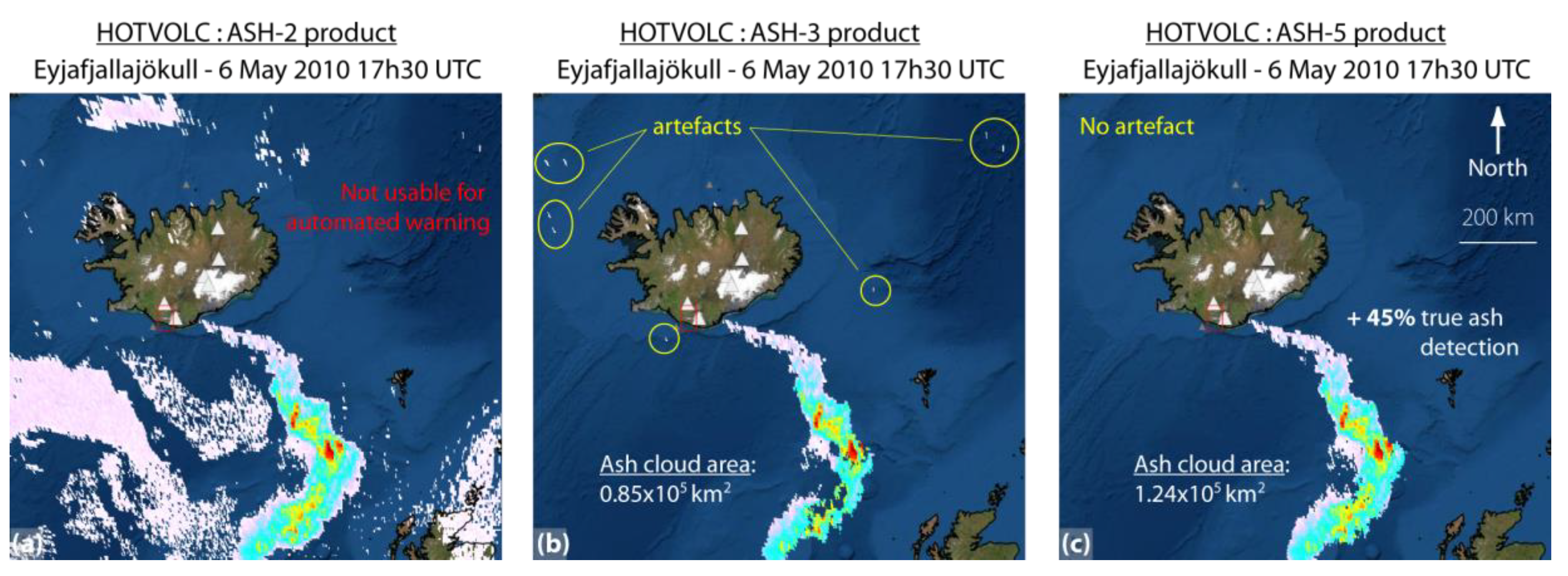
2.1. Ash Cloud Detection (ASH-2, ASH-3, ASH-5)

Thermal infrared (TIR) sensors have proven to be very useful for the operational detection of volcanic ash. They allow reliable 24/7 monitoring of ash clouds, and are the most used sensors today, as they equip all geostationary platforms. In the spectral region of thermal infrared (8–14 µm), we can distinguish silicate particles (i.e., volcanic ash) from other particles such as ice crystals or water and sulphuric acid droplets. This is made possible thanks to the differential extinction properties (i.e., absorption + diffusion) of these particles between the channels located at ~11 µm and ~12 µm [18]. Indeed, the difference in brightness temperature (called BTD) measured at the sensor between these two channels is negative for ash (BTD11-12 < 0) but positive for water and ice (BTD11-12 > 0), and referred to as the 2-bands method. This is the first detection index used in HOTVOLC, hereafter called “ASH-2” product. However, some issues related to this method, summarized in [19], may limit its use for automated detection of volcanic ash. Therefore, more sophisticated techniques have been developed to improve ash characterization and allow automated detection such as the Robust Satellite Technique [20,21,22], the MIR band method [23,24,25], the atmospheric correction [26,27], the VIS–IR daytime method [28] or more recently the 3-Band method [19,29,30,31], which is the second index used in HOTVOLC and referred to as the “ASH-3” product. In this context, we developed a new technique based on 5 spectral bands from MIR and TIR region together and referred to as the “ASH-5” index.
The 5-band algorithm is a bit more complex as it uses several Boolean tests based on either brightness temperature differences (BTD) or spectral radiance for five different infrared bands located at 3.9, 8.7, 10.8, 12, and 13.4 µm. The mid-wave infrared (3.9 µm) allows us to better take into account the solar contribution within ash absorption and scattering using two different thresholds between night and day. Bands at 8.7, 10.8, and 12 µm work as in the 3-band method while the 13.4 µm waveband shows good results for removing artefacts due to convective clouds, in particular. The algorithm is divided into two main parts. The first part uses a very restrictive detection scheme. The objective is to reduce to an absolute minimum the number of false ash detections, hence focusing on the core of the ash cloud:
  • flagged pixels must fill both conditions simultaneously
    BT10.8−BT 12.0 < −0.5 K
    BT 8.7−BT 10.8 > −0.5 K
  • flagged pixels that fill at least one condition are masked
    (RAD3.9−RAD12)/(RAD3.9 + RAD12) < Threshold−(night: 0.042−day: 0.055)
    (BT8.7−BT 12.0)/(BT 10.8−BT 13.4) > −0.05
    ((BT 10.8−BT 12.0)/BT 13.4)) × 100 > −0.35
The second part consists in finding the nearest neighbour to identify closest pixels of the cloud core forming new clusters having a high probability to belong to the ash cloud. Once identified, new Boolean tests are carried out on those pixels:
  • Remaining pixels must fill both conditions simultaneously
    BT10.8−BT 12.0 < −0.25 K
    BT 8.7−BT 10.8 > −2 K
  • Finally, pixels that fill the following condition are masked:
    (RAD3.9−RAD12)/(RAD3.9 + RAD12) < Threshold−(night: 0.042−day: 0.055)
In Figure 2 we provide one example showing differences between the three different algorithms used during the 6 May 2010 Eyjafjallajökull eruption. The 2-band method shows a good sensitivity to ash detection but produces a very large number of false alarms. Those biases can sometimes be overcome from the supervision of a user, but prevent any automated warnings. The 3-band method succeeds in removing most of artefacts, but one can observe that the ash detection sensibility has decreased significantly on the edge of the cloud. Finally, we show that the 5-band method (ASH-5 product) allows removing all artefacts, while increasing the detection sensibility at the same time. Indeed, it improves the detection of ash-bearing pixels by 45% (in terms of cloud area). This good result is due to an original multispectral combination associated with clustering routines. However, those methods remain complementary in some cases and we decided to keep all three in the operational system HOTVOLC.

2.2. “Ash Plume Altitude” Product

Infrared methods also allow the characterization of the ash cloud top altitude, which is critical information for aviation safety. For this purpose, we use the brightness temperature of the cloud surface at 11 µm. This temperature value is then compared to an atmospheric temperature-altitude profile (theoretical or measured from radio-sounding), thus allowing a first order estimation of the cloud altitude. This technique is known as the CTT method (i.e., Cloud Top Temperature) and relies on several assumptions: (i) the cloud must be optically thick (τ > 5) so that the brightness temperature is representative of the true cloud surface temperature. (ii) The ash particles must be in thermal equilibrium with the temperature of the ambient air. (iii) This method is only applicable to tropospheric emissions since the atmospheric temperature profile above the tropopause is not monotonic. It is therefore impossible to obtain a single solution.
The product “Ash-Cloud altitude” provided in HOTVOLC uses the CTT method. Practically, and for operational purposes, we use climatic models to derive temperature-altitude profiles in real-time. There are 4 different models hereafter named midlat_midseason, midlat_summer, midlat_winter, and tropical. For volcanic emissions between −23° and +23° latitude, the tropical profile is used, in other cases middle latitude profiles are used. In this latter case, the date of eruption is used to select between summer, winter or midseason profile.

2.3. “Ash Plume Mass” Product

TIR sensors have proven to be very useful for the operational characterization of volcanic ash cloud. They allow reliable 24/7 detection as demonstrated above from various techniques all using differential extinction properties of silicate particles. Since the 1990s, the quantitative ash concentration was made possible from the inversion of satellite-based TIR data [4,32]. In that aim, a retrieval scheme has been developed and used in HOTVOLC. Inversion of satellite-based TIR data requires the development of a forward electromagnetic (EM) model that realistically accounts for the physics of the problem (i.e., source conditions, EM theory, geometrical setting, etc.). The TIR radiation from Earth is used as the source of energy (here after referred to as the spectral radiance) whose distribution is isotropic in the upper half-space and of constant intensity, at first order. In the presence of an ash cloud, a fraction of this energy is absorbed and scattered by silicate particles according to the Mie theory and does not reach the sensor. [4] Developed a forward model describing the physics of ash cloud characterization from satellite-based IR sensors. They define a linear model of the at-sensor spectral radiance L(λ) such as:
L ( λ ) =   t c ε s B ( λ , T s ) + ε c B ( λ , T c )
  • Ts the brightness temperature of the ground surface
  • Tc the brightness temperature of the cloud top
  • B the Planck function
  • εs the emissivity of the ground surface
  • εc the emissivity of the cloud
  • tc Transmissivity of the cloud
  • L the at-sensor spectral radiance
To solve for the cloud emissivity, the cloud reflectivity (rc) must be added [33] in the above equation so that we can rewrite the at-sensor radiance by a combination of the cloud transmissivity and reflectivity only:
L ( λ ) = ( 1 r c ( r e , τ c ) ) ε s B ( λ , T c ) + t c ( r e , τ c ) ( B ( λ , T s ) B ( λ , T c ) )
A synthetic at-sensor radiance L(λ) can thus be estimated for any wavelengths (Equation (2)) from the calculation of the transmissivity and reflectivity using a Radiative Transfer Model (RTM). The two parameters being a function of the effective radius (re) of the particles and the optical thickness (τc) of the cloud. The calculation of the reflectivity and transmissivity of the medium can be very complex depending on assumption made and boundary conditions. In the case of ash cloud, we have chosen to adapt a two-stream method to solve the radiative transfer equation (RTE):
µ d I d τ = I ( τ , µ ) ω 2 1 1 P ( µ , µ ) I ( τ , µ ) d µ + S ( τ , µ )
where I is the diffuse radiance, µ the cosine of the zenith angle, P(µ,µ’) is the axially-symmetric phase function defining the light incident at µ’ which scattered in the direction µ. τ is the optical depth and ω is the single scattering albedo. The underlying idea is that for a thick plane parallel cloud of ash, the angular distribution of the diffuse radiance does not change radically (i.e., ~isotropic) as in [34]. The strategy is thus to introduce an effective angular-averaged intensity consisting of only two streams (upward I and downward I). The so-called two-stream methods (such as Eddington approximation) provide analytical solutions to the single layer plane-parallel radiative transfer equation. There are many related two-stream methods that approximate the angular radiance field with two numbers (e.g., constant hemisphere [I+, I], two-point quadrature [I(+µ1), I(−µ1)], Eddington 1st moment [I(µ) = I0 + I1µ]). In our conditions of acquisition, two-stream methods give very good results and ensure a fast computational speed. This is a critical point for providing quantitative estimates of the ash concentration in operational fashion. Many versions of two-stream methods exist, and have their own specificities: (i) the ones from [34] or [35] are more adapted to thin ash clouds (τc< 5), while (ii) for thick ash cloud (τc >> 5), the delta-Eddington approximation [36], should be used for direct beam modelling. Assuming that the angular radiance field can be approximated by the two-term Legendre polynomial function, the Eddington approximation is written as follows:
I ( τ , µ ) = I 0 ( τ ) + I 1 ( τ ) µ
In our specific case, the boundary conditions of the problem say that the medium is illuminated from below by a known source of diffuse radiation (i.e., TIR Earth radiation), such as:
I ( 0 , µ , φ ) = + F 0             a n d           I ( τ * , + µ , φ ) = 0    
Then, for a single scattering albedo ϖ < 1, and whatever the cloud thickness (τc), HOTVOLC uses the Eddington approximation, where the reflectivity (R) and transmissivity (T) of the cloud can be written as:
R = ( 1 U 2 ) ( e k τ e k τ ) ( 1 U ) 2 e k τ ( 1 + U ) 2 e k τ   ,                             T = 4 U ( 1 U ) 2 e k τ ( 1 + U ) 2 e k τ
with
U = 4 ( 1 ω ) 3 ( 1 ω g )   ,                   k = ( 1 ω ) ( 1 ω g )
From the calculation of R and T, we solve Equation (2) and provide a synthetic at-sensor radiance pair L(λ1) and L(λ2), by defining the effective radius (re) and the optical depth (τc) defined as:
r e = r 3 n ( r ) d r r 2 n ( r ) d r
τ c = π L 0 r 2 Q e x t ( r , λ ) n ( r ) d r
where Qext is the Mie extinction efficiency. This forward model allows a theoretical look-up table (LUT) to be generated for sets of variations of both re and τc as a function of brightness temperatures (or equivalent radiances). The inverse procedure thus consists in retrieving, by best fit matching, the values of re and τc that correspond to recorded brightness temperature pair. Finally, the total mass of ash particle in a given pixel can be calculated from the integral of the grain size distribution (GSD) of effective radius retrieved. Usually, the GSD used for the LUT generation is polydisperse being either lognormal or modified-gamma distribution. In this case the total mass (in kg) in a pixel is calculated following:
M = L S 4 π 3 ρ 0 r 3 n ( r ) d r
It can be very convenient to express the total mass as a function of the extinction efficiency as the cloud geometric thickness (L) vanishes from the equation in favour of the optical depth (τc) such as:
M = S 4 3 ρ   r e τ c π r 2 n ( r ) d r Q e x t π r 2 n ( r ) d r
Interestingly, for a uniform distribution n(r) = 1, the integrals vanish such that the total mass in a given pixel can simply be written as:
M = S 4 3 Q e x t ρ   r e τ c
IR imager such as SEVIRI provide plane-parallel (2D) images of the ash cloud, and the mass given in a pixel is the sub-vertical integration of particles loading from the ground to the sensor and usually referred to as vertical column densities (VCD). As a result, we can ultimately provide a “surface concentration” of the cloud, usually expressed in g/m2, from the ratio of the total mass over the pixel surface M/S. However, the LUT computing time remains relatively high compared to the METEOSAT acquisition frequency (1 image/15 min), even if the improvement of the computational routines should allow the production of real-time deliverable in near future. In the current version of HOTVOLC, look-up tables are pre-computed from the Eddington approximation for a wide range of standard input parameters (GSD, optical depth, ground BT, emissivity, refractive index, etc.). Then, vertical column densities of ash (referred to as VCD_ash) have been systematically inferred from the inversion of benchmarks case studies (e.g., Etna, Eyjafjallajökull), allowing a simple parameterization of VCD_ash from the ash cloud brightness temperature at 10.8 µm (BT_10.8). Therefore, the computation of first order ash vertical column densities is immediate, expressed in g/m2, and of the form:
V C D _ a s h = α   × e x p ( β × B T _ 10.8 )
where α and β are coefficients obtained by best fit matching, and BT_10.8 is the ash cloud top brightness temperature at 10.8 µm on the satellite image. In reality, the ash cloud has a finite vertical extent, referred to as the geometrical thickness (L), and in cases where it is known, one can derive an average concentration M/LS, usually expressed in mg/m3. However, the thickness of the cloud is quite impossible to obtain in real-time as Lidar transects are scarce. Some studies of plume rise in stable stratified atmospheres (EUM/MTG/DOC/10/0560) suggest that, to a reasonable approximation, the vertical extent of a plume could be estimated from the cloud top height (ztop) following:
L = 0.4 z t o p
However, Lidar distal measurements carried out during the April 2010 Eyjafjallajökull eruption, provide much lower ash cloud thickness estimate of ~1 km [37,38,39,40]. In this case, and in absence of direct Lidar measurements, we suggest using this reference value for the calculation of the average concentration ( C ¯ a s h ) from VCD_ash as follows:
C ¯ a s h = V C D _ a s h / L ¯
with
  L ¯   = 1000   m
For example, a vertical column density of 1 g/m2 homogeneously distributed over 1000 m of thickness gives 1 mg/m3. This approximation probably gives a maximum estimate close to the vent where cloud thickness can be higher. But, since we cannot estimate plume thickness to any greater accuracy, this represents an interesting approach in the context of operational air risk mitigation. A number of explosive eruptions have already been characterized using this methodology developed for the HOTVOLC system: this includes in particular the Eyjafjallajökull 2010, eruption [38], the Etna 2013, eruption, [41] or the Anak-Krakatoa, 2018, eruption [10].
Here we present a new case study (Figure 3) during the 24 December 2018 Etna eruption at 12:15 UTC, in order to show the different HOTVOLC products. Those images are screenshots of the web-GIS interface and have been calculated automatically in real-time. In the first panel, the ASH_5 product allows a clear and unambiguous detection of the ash cloud drifting southeastwardly, right above the Catania international airport, located in the same direction at ~15 km away from the summit craters. The maximum split-window BTD recorded lies around −2.5 K. The vertical column densities (VCD_ash) are provided in the second panel showing a maximum of 6 g/m2 at the end of the plume, and considering an average cloud thickness of 1000 m, one can estimate an ash cloud concentration of ~6 mg/m3, which is well above the threshold value of 4 mg/m3, referenced since 2010 as a “high” level of contamination in the ICAO volcanic ash contingency plan for the EUR/NAT (EURopean and North ATlantic) region. In Figure 3c, the ash cloud top altitude is estimated to be ~7 km a.s.l., which is in fairly good agreement with [42] providing a vertical plume top height in the range 6–8 km at the eruption start from both SEVIRI sensor and ground visible imagery. Similarly, VIIRS satellite data from [43] give a maximum plume top height of 8800 m. In Figure 3d, we show the contour product developed and used by the HOTVOLC system. This is a shape file automatically calculated at each image and producing a contour line around the volcanic ash cloud. This is interesting as it can be compared directly with contours provided on VAG advisories by the Toulouse VAAC.

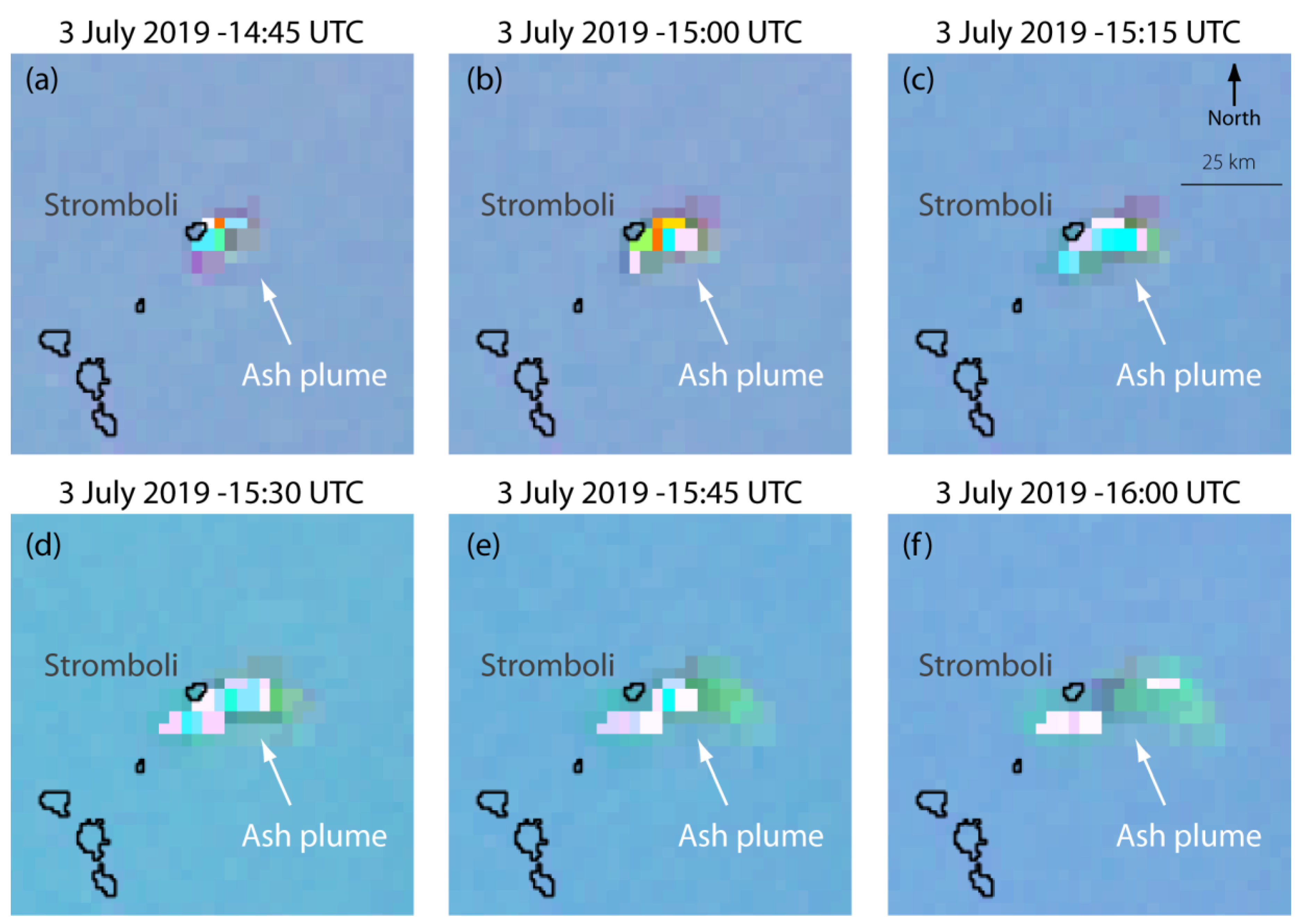
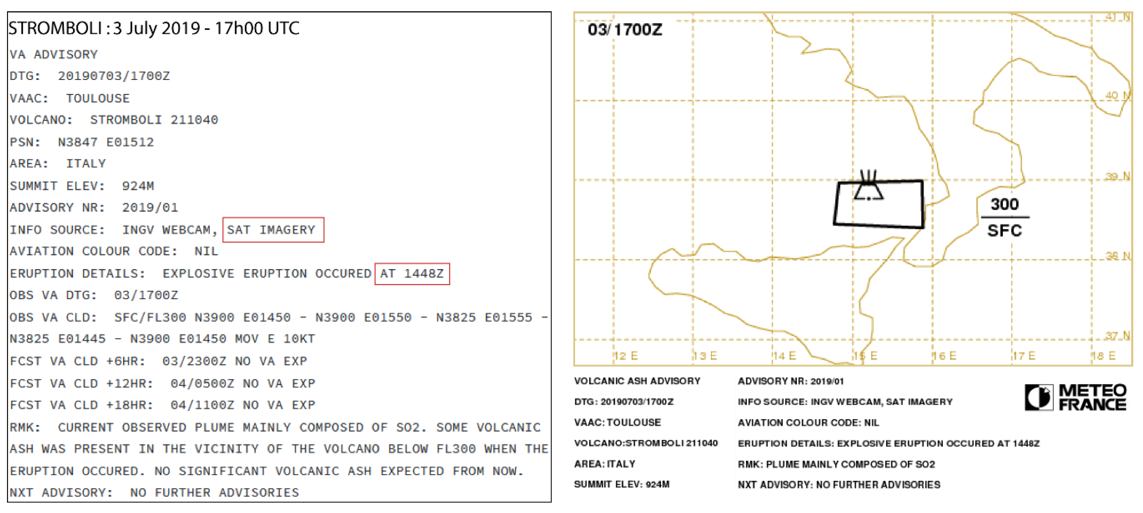
3. Case Study: The 3 July 2019 Stromboli Eruption

Stromboli is a stratovolcano located in the Aeolian Islands (south Italy) culminating at an altitude of 924 m. It is characterized by persistent activity, consisting of mild, so-called Strombolian explosions, occurring several times an hour for more than a millennium. Related pyroclasts ejected consist essentially in black lapilli, scoria and incandescent bombs up to 100–150 m of height above the eruptive vents. The active summit vents are located at the head of the Sciara del Fuoco (750 m a.s.l.), where occasional lava flows pour out, and sometimes reaching the sea. The ordinary explosive activity is interrupted by larger explosions producing ash plumes up to several kilometres high and transported in the atmosphere to distal locations (i.e., few tens of kilometres). These major events are conventionally called “paroxysms” [44] and result from the rise of a deeper volatile-rich low porphyritic magma producing black scoria to yellow pumice with, sometimes, a significant fraction of fine ash [45]. Such events are not uncommon, and have occurred at least three times in the past twenty years in 2003, 2007 and 2019. However, as in 3 July 2019, no precursor has been recorded prior to the paroxysmal explosion taking scientists and inhabitants of the island by surprise. In this context, we show here that satellite-based images can be helpful to trigger the alert and provide timely information on ash cloud concentration and altitude.
HOTVOLC is a real-time monitoring system providing images every 15 min over 50 volcanic targets, including Stromboli. In addition to standard parameters of spectral radiance and temperature, The HOTVOLC system provides high value-added products on lava flow anomalies, sulphur dioxide and ash clouds. Thermal anomalies detected using NTI* (Normalized Thermal Index) refer automatically to an alert by colour code depending on the intensity (i.e., total spectral radiance —TSR) of the lava effusion (green, yellow, red) and is particularly adapted to effusive activity (ex. Piton de la Fournaise). For highly explosive eruption, generating ash plumes, ash indices have been developed to identify ash-bearing pixels, allowing to expert user to trigger the alert.
On 3 July 2019 a giant gas bubble burst at the summit crater of Stromboli at about 14:45 UTC followed by the formation of an ash plume and a strong SO2 emission. However, the Toulouse VAAC did not receive VONA from the volcano observatory and was alerted by a SIGMET (SIGnificant METeorological Information) issued by the Roma Meteorological Watch Office. At the exact same instant, the HOTVOLC system, which is used routinely by Toulouse VAAC, was providing real-time images showing the presence of an ash plume above Stromboli, which confirmed that an eruption was indeed in progress. In Figure 4, we provide 6 successive images (every 15 min) showing the ash plume from the onset of the eruption at 14:45 UTC hence demonstrating the capability of the HOTVOLC system to provide timely information for early warning.
Two different layers are used here: the background is the “Cloud-RGB” product, and the foreground is the “ASH-3” product allowing ash to be identified using a rainbow colorbar. From the image à 15:00 UTC, the ash plume altitude has been estimated to be in the range 4–7 km a.s.l. from the “ash-plume altitude” product, and the ash cloud load has been estimated to be 1–4 g/m2 using the “ash-plume-concentration” product. This information is calculated automatically and provided in real-time on the HOTVOLC interface. Both information are critical as the plume altitude could be used to derive source Mass Eruption Rate (MER) in VATD models such as MOCAGE-Accident run by the Toulouse VAAC. Then, the ash plume concentration products could be used to calibrate and/or validate contamination charts produced by the VAACs in near real-time. HOTVOLC is currently used as visual and qualitative tool by the Toulouse VAAC for decision support, however, automated ingestion of HOTVOLC data products are not implemented yet. It will also be the subject of future developments.
A little later, around 16:00 UTC, the ash cloud was greatly diluted after being transported eastward for barely 2 h. Interestingly, a light green colour on the “Cloud-RGB” product indicates the presence of SO2 in the atmosphere. In Figure 5, we provide the VAA and VAG messages issued by the VAAC of Toulouse during the 3 July 2019 Stromboli eruption. The VAA mentions the eruption start time at 14:48 UTC, which is coherent with the first image detected by HOTVOLC. It also mentions that at 17:00 UTC the plume is mainly composed of SO2 with ash plume present below FL300 (Flight Level 30,000 feet, ~9 km), which is here again very consistent with satellite observations provided by HOTVOLC.

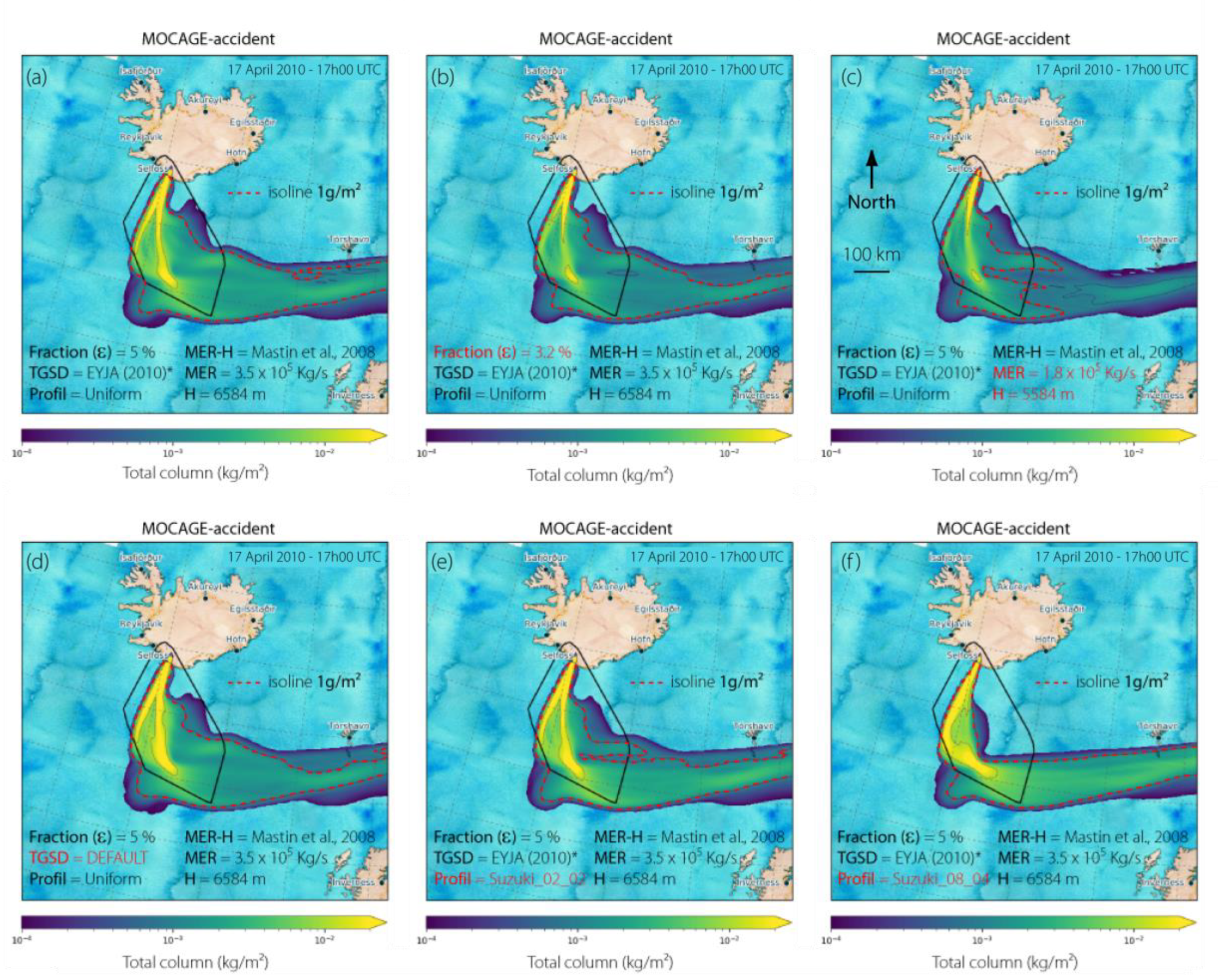
4. MOCAGE-Accident: Parametric Study

MOCAGE-Accident is the global Eulerian dispersion model used by VAAC Toulouse. It is based upon the MOCAGE three-dimensional chemistry and transport model developed by Météo-France for the numerical simulation of the interactions between dynamical, physical and chemical processes in the lower stratosphere and in the troposphere, from the regional to the global scale [46,47]. MOCAGE-Accident is a specific version of MOCAGE, where chemical processes are deactivated, and optimization reinforced, to allow a faster response in operations: the first 12 h of simulation are available within 5 min. It uses an explicit semi-Lagrangian scheme to describe advection, and parameterization schemes to describe turbulent diffusion and convection, as well as scavenging and sedimentation. MOCAGE-Accident runs in off-line mode, using Météo-France ARPEGE or ECMWF/IFS (European Centre for Medium-Range Weather Forecasts) operational NWP products as dynamical forcing. For this study, ARPEGE meteorological data were extracted from Météo-France operational database. The main fields used are the temperature, the humidity, and the wind related fields. These meteorological data include 28 pressure levels, from 1000 to 10 mb, with a time resolution of 3 h, a horizontal resolution of 0.5° for a global domain and a resolution of 0.1° for a nested 60° × 60° domain centred on the eruption. MOCAGE-Accident internal grid resolution is also 0.5° on a global domain, and 0.1° on the nested domain.
In this section, are presented a series of parametric tests on the Eyjafjallajökull 2010, eruption in order to assess the sensitivity of ash column densities forecasted by MOCAGE-Accident. In addition to meteorological data mentioned above, MOCAGE-Accident needs a set of volcanological input parameters, this includes in particular: the Total Grain Size Distribution (TGSD), the ash column profile (ex. uniform, umbrella, etc.), the top plume height (H) and the source Mass Eruption Rate (MER). Practically, it uses observed plume top height to infer the MER from the empirical relationship given by [48]. Then, a partition coefficient (ε) is applied to the source MER (such as ε × MER) in order to take into account the fine ash fraction only, which alone can be transported to distal location in the atmosphere. A variety of output products can be provided by MOCAGE-Accident. It comprises the concentration at different pressure level, total column densities or concentration charts (i.e., with thresholds identified by a colour code). A sensitivity study has been carried out by varying the input parameters in MOCAGE-Accident. In Figure 6, we provide the total vertical column densities (VCD) at the top-of-atmosphere for 6 cases, so that it can be further compared with VCD provided by HOTVOLC data. Input parameters used are summarized in Table 1 and show different configurations of simulation. In particular, we tested a standard partitioning coefficient of ε = 5% and a modified one of 3.2% (case b). According to [49], the latter is assumed to be the best choice for this eruption. The default VAAC operational TGSD is used (case d) as well as a specific TGSD defined for Eyjafjallajökull 2010, eruption from [6]. The ash column profile above vent is set either uniform or umbrella-shaped (case e, f) using the Suzuki parameters [50]. As described above, the formulation from Mastin et al., 2009 is used in all cases, so there is a trade-off between the plume top height and the source MER. The default altitude [51] for April 17 is defined at 5584 m above vent, and leading to a default MER of 3.5 × 10⁵ kg/s. A 1000-m lower value is tested (case c) leading to a MER of 1.8 × 10⁵ kg/s. Resulting maximum VCD corresponding to above-vent values at the top of the ash column are given in Table 1.
Considering case a as a reference with a maximum VCD at 190 g/m2, we can thus compare the effect of each parameter on the maximum VCD. Firstly, one can observe (case c) that a lower ash column of 1000 m decreases by a factor of ~2 the source MER using [48] relationship: the resulting effect on the maximum VCD is thus significant, lying at 91.7 g/m2. This stresses the importance of accurate plume height measurements during the course of an eruption. Secondly, the partitioning coefficient (ε) is not negligible as using 3.2% instead of 5% (case b) decreases significantly the maximum VCD going from 190 to 122 g/m2. Finally, the use of the default TGSD and the umbrella column profile both slightly increase the maximum VCD.
For the production of VCD maps displayed in Figure 6, ash was released continuously from the April 16 at 03:00 UTC using MER and other parameters summarized in Table 1. Each panel represents the situation occurring on April 17 at 17:00 UTC. The shape of the plume and VCD intensities follow the results already described in Table 1 for maximum VCD. Interestingly, we highlighted the 1 g/m2 isoline (red dotted line) in order to better compare the shape of each atmospheric discharge, but also because this value is close to the ash detection threshold of METEOSAT satellite used by HOTVOLC. Unsurprisingly, case c shows the smallest 1 g/m2 envelope, while case f shows the narrowest plume. The black solid line represents the ash cloud contour (using “contour” product) as detected by HOTVOLC at the same instant.

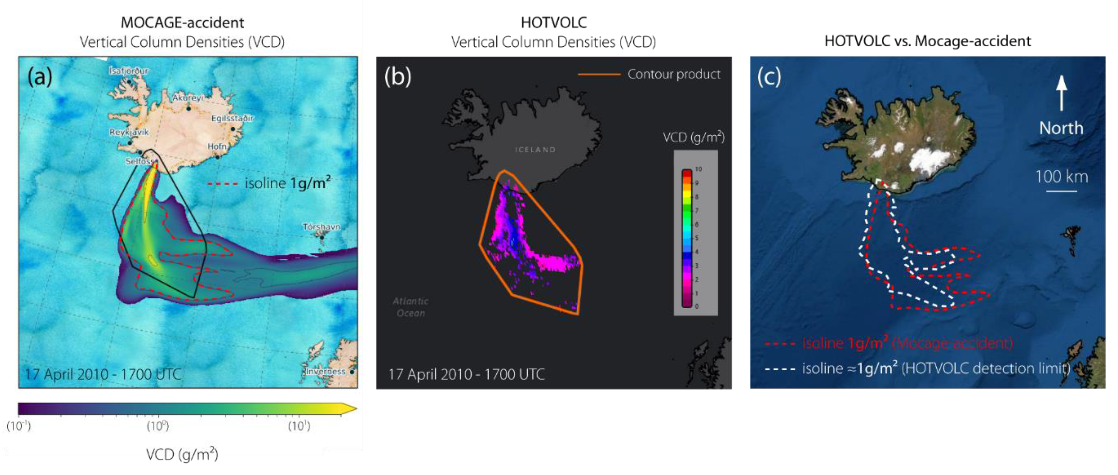
5. HOTVOLC vs. MOCAGE-Accident Comparison

In Figure 7, we made a comparison of the cloud shape and VCD values between one simulation from MOCAGE-Accident and satellite observations from HOTVOLC. Figure 7a stands for the case c (see Table 1 for input parameters used), and represents VCD values of the ash cloud (expressed here in g/m2) on April 17 at 17:00 UTC. The red dotted line represents the threshold envelop at 1 g/m2. The Figure 7b displays the ash cloud VCD calculated from the “VCD_ash” algorithm of HOTVOLC described above, and expressed in g/m2. The image is taken at exactly the same time (17/04 at 17:00 UTC) with VCD values ranging from 1 g/m2 in the outside of the cloud (the most diluted part) to 5 g/m2 in the inside of the cloud (the densest part). This is consistent with most observations of ash clouds, at least close to the eruption site, because ash emissions are produced from a point-source (i.e., the vent). These features are comparable with the VCD map (Figure 7a) produced by MOCAGE-Accident, although showing higher values. Note that close to the vent, no ash was detected from satellite data. At this location we assume that the amount of water droplets (or ice crystals) was significant, leading to positive BTD values, and preventing from any ash detection, whatever the method used. In Figure 7c, the threshold envelope at 1 g/m2 computed by MOCAGE-Accident (red dotted line) is compared, with the interpolated outer envelope from HOTVOLC (white dotted line), approximately lying around the VCD value at 1g/m2 (medium pink pixels in Figure 7b). The comparison shows that both the cloud geometry and quantitative VCD values from modelled and observed data are close. Discrepancies regarding higher modelled VCD values close to the vent and in the central part of the cloud can be explained in two ways: (i) several studies suggest that particles larger than ~30 µm cannot be retrieved from IR satellite techniques [52], thus preventing from ash-rich cloud regions detection. The overall underestimation associated from this issue is estimated to be at least 50% [19,52,53]. (ii) The discrepancy can also be explained by the absence of appropriate sedimentation processes in the model. Indeed, in the proximal regions, fine ash sedimentation can be greatly enhanced due to processes like particle aggregation [54,55,56], or collective settling [49,57]. Neglecting these effects may artificially increase the ash concentration forecasted in the cloud.

6. Conclusions and Discussions

This study shows how the satellite-based system HOTVOLC can help with operational management of explosive volcanic crisis in coordination with the Toulouse VAAC. This is based, in particular, on the ability to provide reliable satellite products and respond in a timely manner.
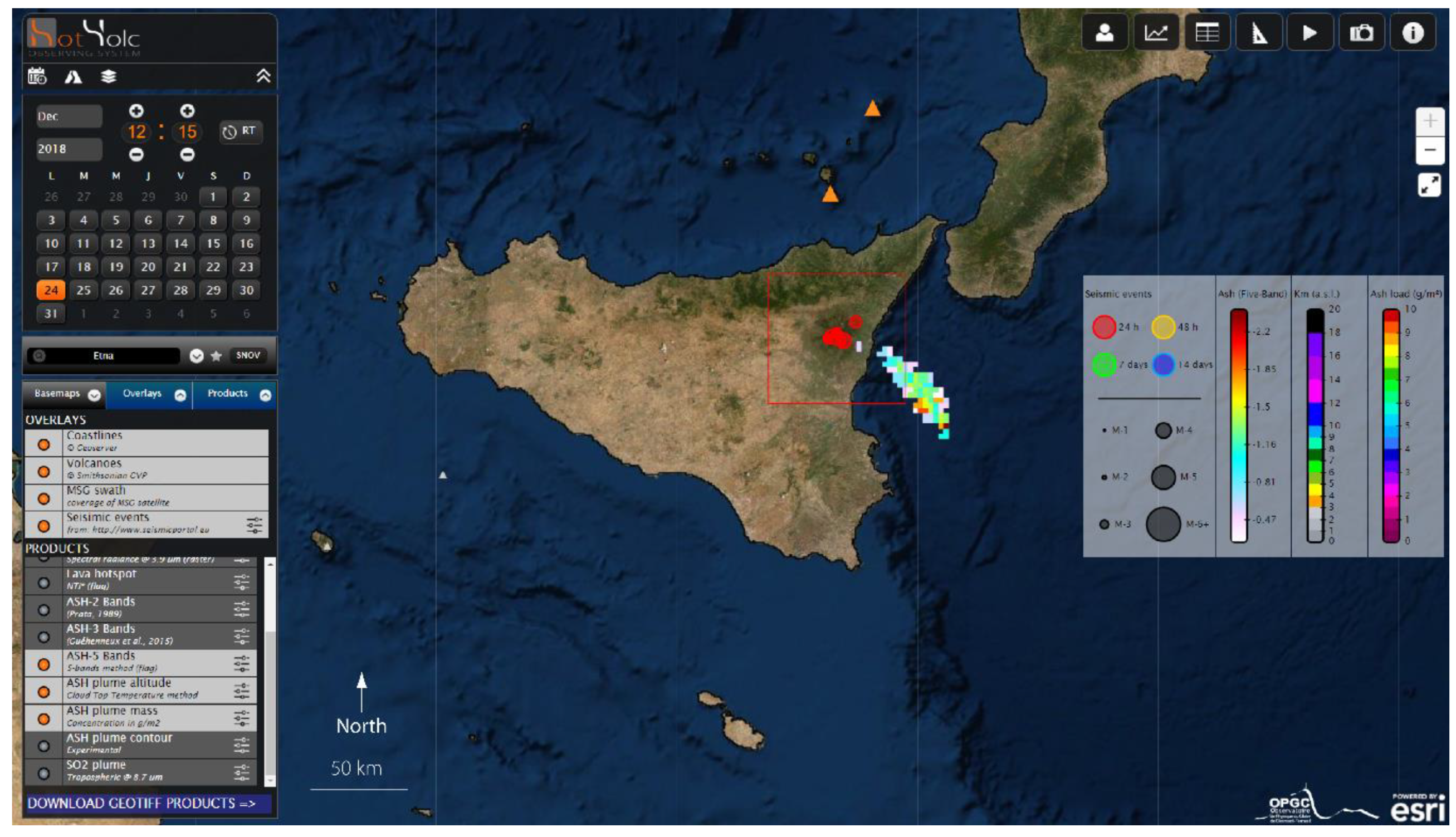
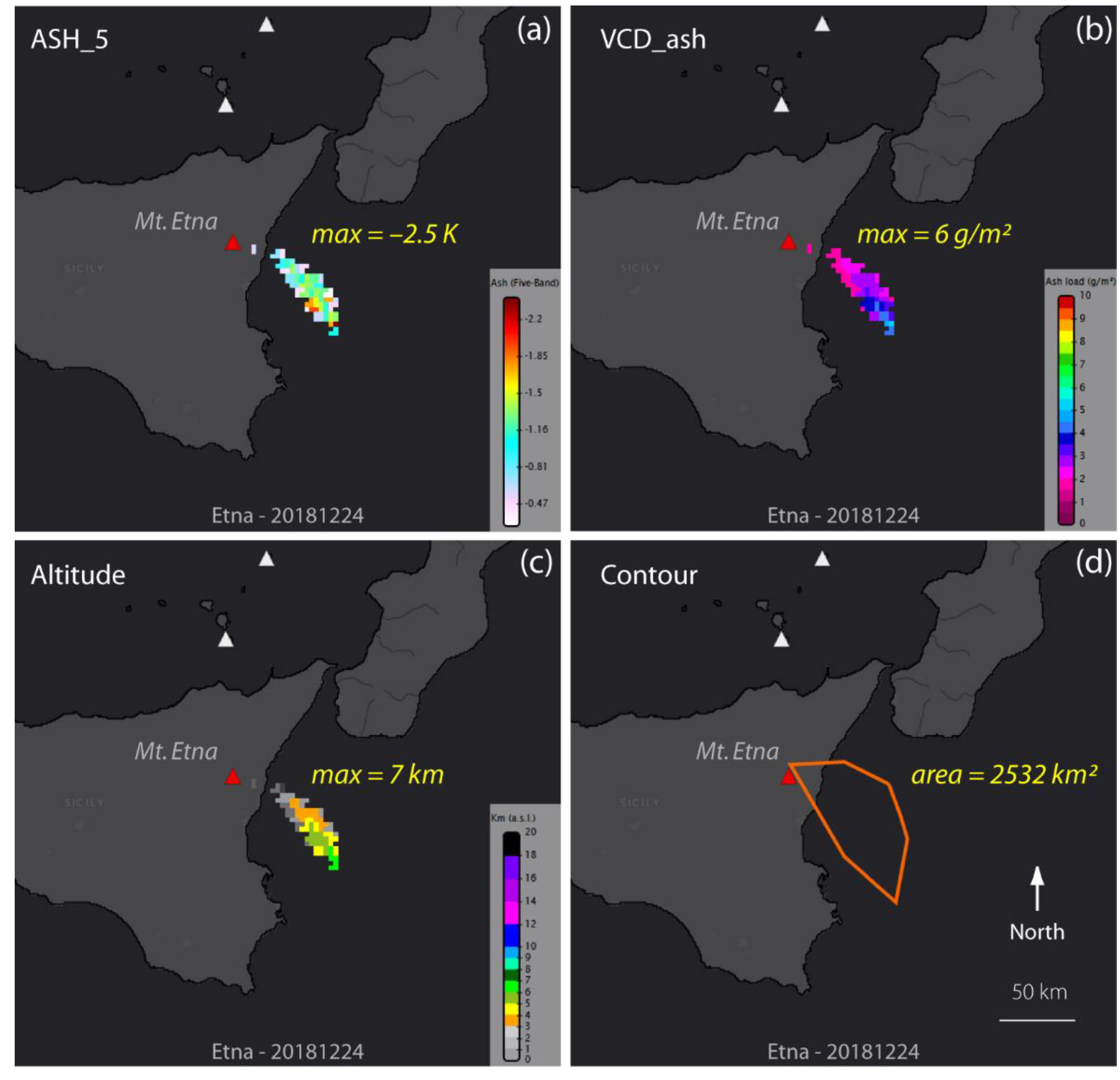
  • Therefore, we first presented newly developed satellite products dedicated to ash clouds retrieval from HOTVOLC system. This includes: (i) “ASH-5 bands” product for improved ash discrimination, (ii) the “ash plume altitude” product providing the top altitude of the cloud, (iii) the “ash plume mass” product that stands for vertical column densities (VCD) and (iv) “ash plume contour” product showing a raw contour line around the cloud. Several eruptions have been characterized using these products, and in this study, we provide new results from the 24 December 2018 Etna eruption. Then, from a detailed sequence of the 3 July 2018 paroxysm at Stromboli, we demonstrate the ability of the HOTVOLC system to react quickly and to assist the Toulouse VAAC in the operational management of the eruptive crisis. This is particularly true at unmonitored volcanoes or when a VONA cannot be issued right in time.
  • In the second part of the study, simulations of ash cloud transport and dispersion have been carried out using MOCAGE-Accident model run by the Toulouse VAAC, during the Eyjafjallajökull eruption on 17 April 2010. The first objective was to assess the model sensitivity to eruption source parameters. For this purpose, we tested a range of input variables of MOCAGE-Accident model, including the Total Grain Size Distribution (TGSD), the eruptive column profile, the top plume height and Mass eruption rate (MER), as well as the fine ash partitioning. Overall, the study of resulting VCD allows us to say that the MER is the parameter having the most impact. Importantly, since MER are inferred from ash column height (H), this means that the estimation of H is critical for the generation of accurate forecast ash maps. Finally, a comparison has been carried out on the same image of Eyjafjallajökull eruption between simulated VCD (from ash dispersion simulations run by MOCAGE-Accident model) and observed VCD (satellite retrieval using HOTVOLC products). In particular, the threshold envelope at 1 g/m2 computed by MOCAGE-Accident (see Figure 7 for input parameters) fits rather well with the one provided from satellite observations.
  • New developments of the HOTVOLC system should be carried in the coming years. This includes in particular (i) the ingestion of atmospheric sounding data or 3D atmospheric weather forecast model. Such improvement must help estimating the ash cloud top altitude (H) by increasing the vertical temperature profile accuracy of the atmosphere. This is particularly important as H controls mostly the MER and hence the ash cloud concentration. (ii) We have shown that VCD can be derived with a relatively good accuracy, but the concentration (in g/m3) along the vertical cloud thickness is much more difficult to estimate, yet it is a critical parameter for aviation safety. For this purpose, the automated ingestion of Lidar transects within HOTVOLC interface should be valuable to better estimate systematically the plume top altitude and the cloud vertical thickness, which are essential for the MER estimation and the vertical concentration, respectively.
  • Finally, the systematic use of the HOTVOLC interface by the Toulouse VAAC will be developed, as it constitutes a valuable help in terms of air risk management. This includes in particular (i) early and unambiguous detection of ash when VONA could not be issued by the volcano observatory (ii) near real-time comparison of observed and forecast ash concentration, cloud altitude and location. (iii) The wide range of eruptions archived on the HOTVOLC system will serve as test cases to train VAAC experts on ash cloud detection and the assessment of its dynamics over time.

Author Contributions

Conceptualization, M.G., P.H., M.D.; Methodology, all authors; software, M.G., M.D., Y.G., B.J.; validation, M.G., M.D., formal analysis, MG., MD., investigation, M.G., M.D., resources, M.D., P.H., P.C., Y.G.; data curation, P.C., Y.G., M.D., writing—original draft preparation, all authors; writing—review and editing, all authors; funding, M.G., P.H.; acquisition, P.C., Y.G., M.D.; All authors have read and agreed to the published version of the manuscript.

Funding

This research was funded by the Centre National d’Études Spatiales (CNES-France), and by the Service National d’Observations en Volcanologie (CNRS-INSU).

Acknowledgments

This work and recent developments of the HOTVOLC system were supported by the Centre National d’Études Spatiales (CNES-France), and by the Service National d’Observations en Volcanologie (CNRS-INSU). We warmly thank the 3 anonymous reviewers for constructive comments.

Conflicts of Interest

The authors declare no conflict of interest.

References

  1. Gouhier, M.; Harris, A.; Calvari, S.; Labazuy, P.; Guéhenneux, Y.; Donnadieu, F.; Valade, S. Lava discharge during Etna’s January 2011 fire fountain tracked using MSG-SEVIRI. Bull. Volcanol. 2012, 74, 787–793. [Google Scholar] [CrossRef]
  2. Furtney, M.A.; Pritchard, M.E.; Biggs, J.; Carn, S.A.; Ebmeier, S.K.; Jay, J.A.; Kilbride, B.T.M.; Reath, K.A. Synthesizing multi-sensor, multi-satellite, multi-decadal datasets for global volcano monitoring. J. Volcanol. Geotherm. Res. 2018, 365, 38–56. [Google Scholar] [CrossRef]
  3. Wright, R.; Flynn, L.P. On the retrieval of lava-flow surface temperatures from infrared satellite data. Geology 2003, 31, 893–896. [Google Scholar] [CrossRef]
  4. Wen, S.; Rose, W.I. Retrieval of sizes and total masses of particles in volcanic clouds using AVHRR bands 4 and 5. J. Geophys. Res. Atmos. 1994, 99, 5421–5431. [Google Scholar] [CrossRef]
  5. Holasek, R.E.; Self, S. GOES weather satellite observations and measurements of the May 18 1994, 1980, Mount St. Helens eruption. J. Geophys. Res. Solid Earth 1995, 100, 8469–8487. [Google Scholar] [CrossRef]
  6. Bonadonna, C.; Genco, R.; Gouhier, M.; Pistolesi, M.; Cioni, R.; Alfano, F.; Hoskuldsson, A.; Ripepe, M. Tephra sedimentation during the 2010 Eyjafjallajökull eruption (Iceland) from deposit, radar, and satellite observations. J. Geophys. Res. Solid Earth 2011, 116. [Google Scholar] [CrossRef]
  7. ICAO EUR/NAT VACP. Volcanic Ash Contingency Plan—European and North Atlantic Regions; Eur Doc 019-NAT Doc 006, Part II; ICAO: Montreal, QC, Canada, 2016. [Google Scholar]
  8. Webley, P.; Mastin, L. Improved prediction and tracking of volcanic ash clouds. J. Volcanol. Geotherm. Res. 2009, 186, 1–9. [Google Scholar] [CrossRef]
  9. Scollo, S.; Prestifilippo, M.; Spata, G.; D’Agostino, M.; Coltelli, M. Monitoring and forecasting Etna volcanic plumes. Nat. Hazards Earth Syst. Sci. 2009, 9, 1573–1585. [Google Scholar] [CrossRef] [Green Version]
  10. Gouhier, M.; Paris, R. SO2 and tephra emissions during the December 22, 2018 Anak Krakatau eruption. Volcanica 2019, 2, 91–103. [Google Scholar]
  11. Casadevall, T.J. (Ed.) Volcanic Ash and Aviation Safety: Proceedings of the First International Symposium on Volcanic Ash and Aviation Safety; US Government Printing Office: Washington, DC, USA, 1994; Volume 2047.
  12. ICAO. The Manual on Volcanic Ash, Radioactive Material and Toxic Chemical Clouds, 3rd ed.; ICAO Doc 9691; Contains Appendix F, Database for Encounters between Aircraft and Ash Clouds; ICAO: Montreal, QC, Canada, 2015. [Google Scholar]
  13. Beckett, F.M.; Witham, C.S.; Leadbetter, S.J.; Crocker, R.; Webster, H.N.; Hort, M.C.; Jones, A.R.; Devenish, B.J.; Thomson, D.J. Atmospheric Dispersion Modelling at the London VAAC: A Review of Developments since the 2010 Eyjafjallajökull Volcano Ash Cloud. Atmosphere 2020, 11, 352. [Google Scholar] [CrossRef] [Green Version]
  14. Gouhier, M.; Guéhenneux, Y.; Labazuy, P.; Cacault, P.; Decriem, J.; Rivet, S. HOTVOLC: A web-based monitoring system for volcanic hot spots. Geol. Soc. Lond. Spec. Publ. 2016, 426, 223–241. [Google Scholar] [CrossRef]
  15. Hampton, S.J.; Cole, J.W.; Wilson, G.; Wilson, T.M.; Broom, S. Volcanic ashfall accumulation and loading on gutters and pitched roofs from laboratory empirical experiments: Implications for risk assessment. J. Volcanol. Geotherm. Res. 2015, 304, 237–252. [Google Scholar] [CrossRef]
  16. Wilson, T.M.; Jenkins, S.; Stewart, C. Impacts from volcanic ash fall. In Volcanic Hazards, Risks and Disasters; Elsevier: Amsterdam, The Netherlands, 2015; pp. 47–86. [Google Scholar]
  17. Josse, B.; Simon, P.; Peuch, V.H. Radon global simulations with the multiscale chemistry and transport model MOCAGE. Tellus B Chem. Phys. Meteorol. 2004, 56, 339–356. [Google Scholar] [CrossRef]
  18. Prata, A.J. Infrared radiative transfer calculations for volcanic ash clouds. Geophys. Res. Lett. 1989, 16, 1293–1296. [Google Scholar] [CrossRef]
  19. Guéhenneux, Y.; Gouhier, M.; Labazuy, P. Improved space borne detection of volcanic ash for real-time monitoring using 3-Band method. J. Volcanol. Geotherm. Res. 2015, 293, 25–45. [Google Scholar] [CrossRef]
  20. Tramutoli, V. Robust AVHRR Techniques (RAT) for environmental monitoring: Theory and applications. In Earth Surface Remote Sensing II; International Society for Optics and Photonics: Bellingham, WA, USA, 1998; Volume 3496, pp. 101–113. [Google Scholar] [CrossRef]
  21. Pergola, N.; Pietrapertosa, C.; Lacava, T.; Tramutoli, V. Robust satellite technique for volcanic eruptions monitoring. Ann. Geophys. 2001, 44, 167–177. [Google Scholar] [CrossRef]
  22. Pergola, N.; Tramutoli, V.; Marchese, F.; Scaffidi, I.; Lacava, T. Improving volcanic ash cloud detection by a robust satellite technique. Remote Sens. Environ. 2004, 90, 1–22. [Google Scholar] [CrossRef]
  23. Ellrod, G.P.; Connel, B.H. Improvements in volcanic ash detection using GOES multispectral image data, Preprint volume 8th Conference on Aviation Range an Aerospace Meteorology. Am. Meteorol. Soc. 1999, 1, 326–329. [Google Scholar]
  24. Mosher, F.R. Four Channel Volcanic Ash Detection Algorithm. Aviation Weather Center Staff Publication.Navigation of AVHRR scheme: Accuracy assessment and validation. Remote Sens. Environ. 1999, 85, 190–203. [Google Scholar] [CrossRef]
  25. Ellrod, G.P.; Connell, B.H.; Hillger, D.W. Improved detection of airborne volcanic ash using multispectral infrared satellite data. J. Geophys. Res. 2003, 108, 4356. [Google Scholar] [CrossRef] [Green Version]
  26. Prata, A.J.; Grant, I.F. Retrieval of microphysical and morphological properties of volcanic ash clouds from satellite data: Application to Mt Ruapehu New Zealand. Q. J. R. Meteorol. Soc. 2001, 127, 2153–2179. [Google Scholar] [CrossRef]
  27. Yu, T.; Rose, W.I.; Prata, A.J. Atmospheric correction for satellite-based volcanic ash mapping and retrievals using “split window” IR data from GOES and AVHRR. J. Geophys. Res. 2002, 107, AAC-10. [Google Scholar] [CrossRef]
  28. Pavolonis, M.J.; Feltz, W.F.; Heidinger, A.K.; Gallina, G.M. A daytime complement to the reverse absorption technique for improved automated detection of volcanic ash. J. Atmos. Ocean. Technol. 2006, 23, 1422. [Google Scholar] [CrossRef]
  29. Pavolonis, M.J. Advances in extracting cloud composition information from spaceborne infrared radiance—A robust alternative to brightness temperature, PART I: THEORY. J. Appl. Meteorol. Climatol. 2010, 49, 1992–2012. [Google Scholar] [CrossRef]
  30. Pavolonis, M.J.; Sieglaff, J. GOES-R Advanced Baseline Imager (ABI) Algorithm Theoretical Basis Document for Volcanic Ash: Detection and Height, Version 2.0, Report; NOAA: Silver Spring, MD, USA, 2010; p. 72. Available online: http://www.goes-r.gov/products/ATBDs/baselined/Aviation_VolAsh_v2.0_no_color.pdf (accessed on 12 August 2020).
  31. Francis, P.N.; Cooke, M.C.; Saunders, R.W. Retrieval of physical properties of volcanic ash using Meteosat: A case study from 2010 Eyjafjallajökull eruption. J. Geophys. Res. 2012, 117, D00U09. [Google Scholar] [CrossRef]
  32. Prata, A.J. Observations of volcanic ash clouds in the 10–12 μm window using AVHRR/2 data. Int. J. Remote Sens. 1989, 10, 751–761. [Google Scholar] [CrossRef]
  33. Watson, I.M.; Realmuto, V.J.; Rose, W.I.; Prata, A.J.; Bluth, G.J.; Gu, Y.; Bader, C.E.; Yu, T. Thermal infrared remote sensing of volcanic emissions using the moderate resolution imaging spectroradiometer. J. Volcanol. Geotherm. Res. 2004, 135, 75–89. [Google Scholar] [CrossRef]
  34. Sagan, C.; Pollack, J.B. Anisotropic nonconservative scattering and the clouds of Venus. J. Geophys. Res. 1967, 72, 469–477. [Google Scholar] [CrossRef]
  35. Coakley, J.A., Jr.; Chylek, P. The two-stream approximation in radiative transfer: Including the angle of the incident radiation. J. Atmos. Sci. 1975, 32, 409–418. [Google Scholar] [CrossRef] [Green Version]
  36. Joseph, J.H.; Wiscombe, W.J.; Weinman, J.A. The delta-Eddington approximation for radiative flux transfer. J. Atmos. Sci. 1976, 33, 2452–2459. [Google Scholar] [CrossRef]
  37. Chazette, P.; Bocquet, M.; Royer, P.; Winiarek, V.; Raut, J.C.; Labazuy, P.; Gouhier, M.; Lardier, M.; Cariou, J.P. Eyjafjallajökull ash concentrations derived from both lidar and modeling. J. Geophys. Res. Atmos. 2012, 117. [Google Scholar] [CrossRef] [Green Version]
  38. Labazuy, P.; Gouhier, M.; Harris, A.; Guéhenneux, Y.; Hervo, M.; Bergès, J.C.; Fréville, P.; Cacault, P.; Rivet, S. Near real-time monitoring of the April–May 2010 Eyjafjallajökull ash cloud: An example of a web-based, satellite data-driven, reporting system. Int. J. Environ. Pollut. 2012, 48, 262–272. [Google Scholar] [CrossRef]
  39. Hervo, M.; Quennehen, B.; Kristiansen, N.I.; Boulon, J.; Stohl, A.; Fréville, P.; Pichon, J.M.; Picard, D.; Labazuy, P.; Gouhier, M.; et al. Physical and optical properties of 2010 Eyjafjallajökull volcanic eruption aerosol: Ground-based, Lidar and airborne measurements in France. Open Archive HAL 2012. [Google Scholar] [CrossRef] [Green Version]
  40. Dacre, H.F.; Grant, A.L.M.; Harvey, N.J.; Thomson, D.J.; Webster, H.N.; Marenco, F. Volcanic ash layer depth: Processes and mechanisms. Geophys. Res. Lett. 2015, 42, 637–645. [Google Scholar] [CrossRef] [Green Version]
  41. Poret, M.; Costa, A.; Andronico, D.; Scollo, S.; Gouhier, M.; Cristaldi, A. Modeling Eruption Source Parameters by Integrating Field, Ground-Based, and Satellite-Based Measurements: The Case of the 23 February 2013 Etna Paroxysm. J. Geophys. Res. Solid Earth 2018, 123, 5427–5450. [Google Scholar] [CrossRef]
  42. Corradini, S.; Guerrieri, L.; Stelitano, D.; Salerno, G.; Scollo, S.; Merucci, L.; Prestifilippo, M.; Musacchio, M.; Silvestri, M.; Lombardo, V.; et al. Near Real-Time Monitoring of the Christmas 2018 Etna Eruption Using SEVIRI and Products Validation. Remote Sens. 2020, 12, 1336. [Google Scholar] [CrossRef] [Green Version]
  43. Calvari, S.; Bilotta, G.; Bonaccorso, A.; Caltabiano, T.; Cappello, A.; Corradino, C.; Del Negro, C.; Ganci, G.; Neri, M.; Pecora, E.; et al. The VEI 2 Christmas 2018 Etna Eruption: A Small but Intense Eruptive Event or the Starting Phase of a Larger One? Remote Sens. 2020, 12, 905. [Google Scholar] [CrossRef] [Green Version]
  44. Bertagnini, A.; Di Roberto, A.; Pompilio, M. Paroxysmal activity at Stromboli: Lessons from the past. Bull. Volcanol. 2011, 73, 1229–1243. [Google Scholar] [CrossRef]
  45. Andronico, D.; Pistolesi, M. The November 2009 paroxysmal explosions at Stromboli. J. Volcanol. Geotherm. Res. 2010, 196, 120–125. [Google Scholar] [CrossRef]
  46. Josse, B. Représentation des Processus de Transport et de Lessivage Pour la Modélisation de la Composition Chimique de L’atmosphère à L’échelle Planétaire. Ph.D. Thesis, Université Paul Sabatier, Toulouse, France, 2004. [Google Scholar]
  47. Sič, B.; El Amraoui, L.; Marécal, V.; Josse, B.; Arteta, J.; Guth, J.; Joly, M.; Hamer, P.D. Modelling of primary aerosols in the chemical transport model MOCAGE: Development and evaluation of aerosol physical parameterizations. Geosci. Model Dev. 2015, 8, 381. [Google Scholar] [CrossRef] [Green Version]
  48. Mastin, L.G.; Guffanti, M.; Servranckx, R.; Webley, P.; Barsotti, S.; Dean, K.; Durant, A.; Ewert, J.W.; Neri, A.; Rose, W.I.; et al. A multidisciplinary effort to assign realistic source parameters to models of volcanic ash-cloud transport and dispersion during eruptions. J. Volcanol. Geotherm. Res. 2009, 186, 10–21. [Google Scholar] [CrossRef]
  49. Gouhier, M.; Eychenne, J.; Azzaoui, N.; Guillin, A.; Deslandes, M.; Poret, M.; Costa, A.; Husson, P. Low efficiency of large volcanic eruptions in transporting very fine ash into the atmosphere. Sci. Rep. 2019, 9, 1–12. [Google Scholar] [CrossRef] [PubMed]
  50. Pfeiffer, T.; Costa, A.; Macedonio, G. A model for the numerical simulation of tephra fall deposits. J. Volcanol. Geotherm. Res. 2005, 140, 273–294. [Google Scholar] [CrossRef]
  51. Webster, H.N.; Thomson, D.J.; Johnson, B.T.; Heard, I.P.C.; Turnbull, K.; Marenco, F.; Kristiansen, N.I.; Dorsey, J.; Minikin, A.; Weinzierl, B.; et al. Operational prediction of ash concentrations in the distal volcanic cloud from the 2010 Eyjafjallajökull eruption. J. Geophys. Res. Atmos. 2012, 117. [Google Scholar] [CrossRef] [Green Version]
  52. Stevenson, J.A.; Millington, S.C.; Beckett, F.M.; Swindles, G.T.; Thordarson, T. Big grains go far: Understanding the discrepancy between tephrochronology and satellite infrared measurements of volcanic ash. Atmos. Meas. Tech. 2015, 8, 2069–2091. [Google Scholar] [CrossRef] [Green Version]
  53. Corradini, S.; Spinetti, C.; Carboni, E.; Tirelli, C.; Buongiorno, M.F.; Pugnaghi, S.; Gangale, G. Mt. Etna tropospheric ash retrieval and sensitivity analysis using Moderate Resolution Imaging Spectroradiometer measurements. J. Appl. Remote Sens. 2008, 2, 023550. [Google Scholar] [CrossRef]
  54. Rose, W.I.; Durant, A.J. Fate of volcanic ash: Aggregation and fallout. Geology 2011, 39, 895–896. [Google Scholar] [CrossRef]
  55. Brown, R.J.; Bonadonna, C.; Durant, A.J. A review of volcanic ash aggregation. Phys. Chem. Earth Parts A/B/C 2012, 45, 65–78. [Google Scholar] [CrossRef] [Green Version]
  56. Van Eaton, A.R.; Mastin, L.G.; Herzog, M.; Schwaiger, H.F.; Schneider, D.J.; Wallace, K.L.; Clarke, A.B. Hail formation triggers rapid ash aggregation in volcanic plumes. Nat. Commun. 2015, 6, 1–7. [Google Scholar] [CrossRef]
  57. Carazzo, G.; Jellinek, A.M. A new view of the dynamics, stability and longevity of volcanic clouds. Earth Planet. Sci. Lett. 2012, 325, 39–51. [Google Scholar] [CrossRef]
Figure 1. Screenshot of the HOTVOLC interface centred on Mount Etna (Sicily) during the 24 December 2018 eruption and showing the ash cloud from various products (ASH-5, altitude, vertical column densities (VCD)) as well as the location of seismic events (red circles).
Atmosphere 11 00864 g001
Figure 2. Maps of ash cloud detected during the 6 May 2010 Eyjafjallajökull eruption at 17:30 UTC using the (a) 2-band, (b) 3-band, and (c) 5-band methods, respectively.
Atmosphere 11 00864 g002
Figure 3. Ash cloud satellite products provided by the HOTVOLC system during the 24 December 2018 eruption and showing (a) the brightness temperature difference (in degree K) using ASH-5 detection product, (b) the vertical column density (VCD_ash) that provide a measure of ash loading in the cloud (in g/m2), then (c) the top ash cloud altitude (in km a.s.l.) and finally (d) the cloud contour.
Atmosphere 11 00864 g003
Figure 4. Ash cloud detected by the HOTVOLC system using the ASH-3 product during the 3 July 2019 Stromboli eruption from (a) 14h45 UTC: start of the eruption, (b) 15h00 UTC: maximum concentration, (c) 15h15 UTC, (d) 15h30 UTC, (e) 15h45 UTC, (f) 16h00 UTC.
Atmosphere 11 00864 g004
Figure 5. VAA and VAG issued by Toulouse VAAC during the 3 July 2019 Stromboli eruption.
Atmosphere 11 00864 g005
Figure 6. Simulations of ash cloud transport and dispersion using MOCAGE-Accident model during the Eyjafjallajökull eruption on 17 April 2010 at 17:00 UTC. (af) Each run uses different input parameters summarized in the image (and in Table 1). Ash cloud colours represent the total column (kg/m2) and also referred to as VCD.
Atmosphere 11 00864 g006
Figure 7. Comparisons of VCD values (in g/m2) between (a) ash dispersion simulations run by MOCAGE-Accident model and (b) satellite retrieval using HOTVOLC products. (c) Superposition of the 1 g/m2 envelope from both methods.
Atmosphere 11 00864 g007
Table 1. Summary of MOCAGE-Accident simulation inputs and outputs.
CaseFraction (%)TGSDProfilePlume Height (m)MER (Kg/s)Max VCD (g/m2)
a5Eyjafjallajökull 2010 Uniform65843.5 × 105190
b3.2Eyjafjallajökull 2010 Uniform65843.5 × 105122
c5Eyjafjallajökull 2010 Uniform55841.8 × 10591.7
d5DefaultUniform65843.5 × 105199
e5Eyjafjallajökull 2010 Umbrella (S_02_02) 65843.5 × 105192
f5Eyjafjallajökull 2010 Umbrella (S_08_04)65843.5 × 105206

