Modeling Emissions from Concentrated Sources into Large-Scale Models: Theory and apriori Testing

Abstract

This paper presents a general procedure to incorporate the effects emissions from localized sources, such as aircraft or ship engines, into chemical transport models (CTM). In this procedure, the species concentrations in each grid box of a CTM are split into plume or small-scale concentrations and background concentrations, respectively, and the corresponding conservation equations are derived. The plume concentrations can be interpreted as subgrid contributions for the CTM grid-box averaged concentrations. The chemical reactions occurring inside the plume are parameterized by introducing suitable “effective” reaction rates rather than modifying the emission indices of the species inside the plume. Various methods for implementation into large-scale models are discussed that differ by the accuracy of the description of plume process. The mathematical consistency of the method is verified on simple idealized setting consisting of a reactive plume in homogeneous turbulence.

1. Introduction

Three-dimensional chemistry transport models (CTM) and climate chemistry models (CCM) are routinely used to evaluate the impact of anthropogenic emissions on the global atmospheric composition. In these models, the emissions are typically represented as grid-averaged quantities that are instantaneously and uniformly distributed within each grid-box of the computational domain. The spatial distribution of exhausts and their physical and chemical transformations are then neglected at subgrid-scale level, which, in turn, can bias the prediction of perturbations that are induced by concentrated or line-shaped emissions, such as in aircraft [1,2], and ship [3] plumes whose characteristic temporal and spatial scales are several order of magnitude smaller than background air. It is known, for example, that, when aircraft ${\mathrm{NO}}_x$ emissions are instantaneously diluted to the scale of CTM grid-boxes, the resulting ozone production can be overestimated by 20% because of the missing conversion of ${\mathrm{NO}}_x$ into nitrogen reservoir species, like ${\mathrm{HNO}}_3$ and ${\mathrm{H}}_2{\mathrm{O}}_5$ [4,5,6,7].

In the literature, various methods have been developed to include the effect of line-shaped emissions (mostly aircraft emissions) into global models [8]. The common idea of these methods is to modify the emission rates i.e., the source terms in the species conservation equations- by means of suitable factors that parameterize the small-scale plume transformations. The first methods to be developed were the Effective Emission Indices (EEI) [9] and the Emission Conversion Factors (ECF) [5,10]. In the EEI method, the correction is directly made at emission time by changing the original emission index $EI$ “as if” an equivalent emission were instantaneously dispersed at large scale. In the ECF method, the emissions are rescaled by the excess of concentrations over background at the end of the plume lifetime. The ECF method has been widely implemented in various CTM to estimate the impact of aircraft emissions on regional [6] and global scales [5,7], and different techniques have been proposed afterwards in order to improve the parameterizations of small-scale chemistry and microphysics [11,12,13,14]. One shortcoming of both EEI and ECF methods is that mass conservation is not automatically guaranteed in the CTM because the source terms in the large-scale conservation equations are modified using external data, so that additional corrections (that are case-dependent) have to be made to fix this problem. The method of effective reaction rates (ERR) was introduced later by [8,15] to represent the chemical conversion of emissions into global models and specifically to study the impact of ${\mathrm{NO}}_x$ emissions on the atmospheric ozone. The basic idea of the method is that the chemical transformations in the plume proceed with different rates than in the background atmosphere, because of the high concentrations of exhausts within the plume. It is then possible to define effective reaction rates working on the fraction of the emissions within the plume (undiluted fraction). The plume effects on a subgrid scale are represented via a fuel tracer in order to follow the amount of the emitted species in the plume and an effective reaction rate for the ozone production and nitric acid production and destruction during the plume dilution in the background. The ERR method has been applied to other scenarios, like ship emissions [16] and lightning [17], and provide more realistic results of the effect of dilution at the grid-scale. While the ERR method guarantees a more consistent relation between the diluted and undiluted contributions of transported species, their conservation laws were given directly in the CTM context with no derivation from first principles. The objective of this work is (i) to present a theory for the derivation of conservation equations used in the ERR method and provide possible generalizations and (ii) to verify the consistency of the model a posteriori which means comparing the model results with those obtained in ideal controlled setting where all the chemical species, velocities field and temperature be determined exactly, which, of course, impossible in a CTM model. It is worth pointing out that the method presented here, either ERR, EEI, and ECF methods, are all parameterizations, i.e., they do not attempt to reproduce the evolution of a given exhaust plume, but rather they mimic the large-scale effects of emissions in such a way that a finite (usually small) number of parameters can be easily incorporated into global models. In this respect, they should not be confused with the methods used in air quality, community, such as plume-in-grid models [18,19], which treat the local impact of emissions from point sources, and represent the plume an ensemble of puffs with complex internal structure.

2. General Formulation of Chemical Transport Models

Consider the conservation equations for a mixture of $N_s$ reacting species,

$$\frac{\partial C_k}{\partial t}+\mathsf{\nabla }·\left(C_k\mathbf{u}\right)+\mathsf{\nabla }·(D\mathsf{\nabla }{C}_k)={\omega }_k+E_k$$

(1)

where $C_k$ is the concentration of species k, D is the (molecular) diffusion coefficient, $E_k$ is the emission rate of species k, while ${\omega }_k$ is the chemical source term:

$${\omega }_k=\sum _{j=1}^{N_r}\mathsf{\Delta }{\nu }_{k_j}{K}_j\prod _{i=1}^{N_s}{c}_j^{{\nu }_{i_j}^{\to }}$$

(2)

where $N_r$ is the number of reactions j that contribute to the production/destruction of species k through reaction rate $K_j$, ${\nu }_{i_j}^{\to }$ (${\nu }_{i_j}^{\leftarrow }$) is the stoichiometric coefficient of species i in the forward (backward) reaction j and $\mathsf{\Delta }{\nu }_{k_j}={\nu }_{k_j}^{\to }-{\nu }_{k_j}^{\leftarrow }$.

In large-scale atmospheric flow simulations, one only knows averaged or filtered variables $\overline{\phi }\left(\mathbf{x}\right)$ that can be generally defined by:

$$\overline{\phi }(\mathbf{x},t)={\int }_{Vol}{G}_{\mathbf{x}}^{\mathsf{\Delta }}\left({\mathbf{x}}^{\prime }\right)\phi ({\mathbf{x}}^{\prime },t)d{\mathbf{x}}^{\prime }$$

(3)

where $Vol$ is the volume of the computational domain and $G_{\mathbf{x}}^{\mathsf{\Delta }}$ is a generic grid-filter operator; for example, using the box filter $G_{\mathbf{x}}^{\mathsf{\Delta }}\left({\mathbf{x}}^{\prime }\right)\equiv {\displaystyle \frac{1}{V}}{\prod }_{i=1}^{3}H\left({\displaystyle \frac{{\mathsf{\Delta }}_i}{2}}-|x_i^{\prime }-x_i|\right)$, where H is the piecewise Heaviside function located at the center $\mathbf{x}$ of a cell of volume $V={\mathsf{\Delta }}_i{\mathsf{\Delta }}_j{\mathsf{\Delta }}_k$ [20], gives the usual volume average:

$$\overline{\phi }(\mathbf{x},t)={\int }_{Vol}{G}_{\mathbf{x}}^{\mathsf{\Delta }}\left({\mathbf{x}}^{\prime }\right)\phi ({\mathbf{x}}^{\prime },t)d{\mathbf{x}}^{\prime }=\frac{1}{V}{\int }_V\phi ({\mathbf{x}}^{\prime },t)d{\mathbf{x}}^{\prime }.$$

(4)

Applying the operator defined by Equation (4) to Equation (1) yields (assuming commutativity):

$$\begin{array}{ccc}\hfill \frac{\partial \overline{C_k}}{\partial t}+\mathsf{\nabla }·\left(\overline{C_k}\overline{\mathbf{u}}\right)+\mathsf{\nabla }·(D\mathsf{\nabla }\overline{C_k})& +& \mathsf{\nabla }·(\overline{C_k\mathbf{u}}-\overline{C_k}\overline{\mathbf{u}})=\hfill \\ & =& \overline{{\omega }_k}+\overline{E_k}\hfill \end{array}$$

(5)

where all of the average variables are now supported by the CTM grid, while subgrid-scale correlations and source terms need to be modeled. For example, the correlation $\overline{C_k\mathbf{u}}-\overline{C_k}\overline{\mathbf{u}}$ is typically modeled using turbulent diffusion and eddy-viscosity concepts:

$$\mathsf{\nabla }·(\overline{C_k\mathbf{u}}-\overline{C_k}\overline{\mathbf{u}})=\mathsf{\nabla }·(D_{turb}\mathsf{\nabla }\overline{C_k}).$$

(6)

Defining $D_t=D+D_{turb}$ (in practice, $D_t\simeq D_{turb}$ since $D\ll D_{turb}$ in atmospheric flows) yields

$$\frac{\partial \overline{C_k}}{\partial t}+\mathsf{\nabla }·\left(\overline{C_k}\overline{\mathbf{u}}\right)+\mathsf{\nabla }·(D_t\mathsf{\nabla }\overline{C_k})=\overline{{\omega }_k}+\overline{E_k}.$$

(7)

Standard inventories of aircraft or ship emissions generally provide for each species k the (time-averaged) sources along prescribed air or see corridors in the form

$$E_k\left({\mathbf{x}}^{\prime }\right)\equiv E{I}_k{S}_F\left({\mathbf{x}}^{\prime }\right)$$

(8)

where $E{I}_k$ is the species emission index at nozzle exit and $S_F\left[\mathrm{Kg}\left(\mathrm{fuel}\right)/\mathrm{s}\right]$ is the mass of fuel burnt per unit volume and time. In chemical transport models, these “scattered” sources are reconstructed as grid-averaged sources $\overline{E_k}$ in Equation (19):

$$\overline{E_k}\left(\mathbf{x}\right)=\frac{1}{V}{\int }_V{E}_k\left({\mathbf{x}}^{\prime }\right)d\left({\mathbf{x}}^{\prime }\right)=E{I}_k\overline{S_F}\left(\mathbf{x}\right).$$

(9)

In the following, a more general closure for these correlations in the presence of concentrated emissions is discussed together with the treatment of the correlations that arise in the source terms ${\omega }_k$ of the right-hand side of Equation (7).

3. Parameterization of Subgrid-Scale Processes into Large-Scale Models: General Formulation

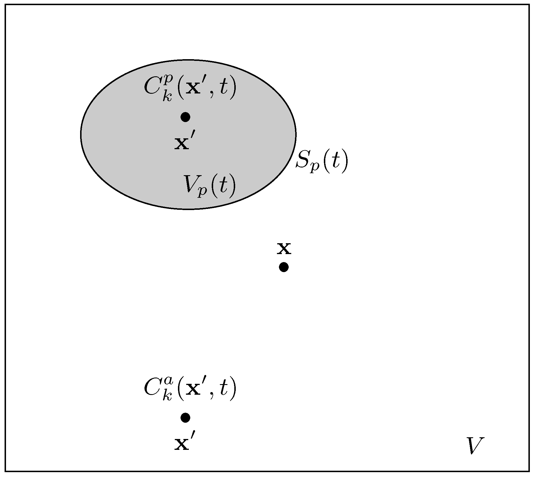
Emissions from a local source inside the computational cell of a large-scale CTM may be represented by a plume of volume $V_p$ separated from background by a (time-evolving) interface defined by the surface $S_p\left(t\right)=0$ (see Figure 1). The contributions from plume ($C_k^p$) and background ($C_k^a$) to the grid-average concentration $\overline{C_k}$ may be identified through the formal definitions:

$$\begin{array}{c}\hfill C_k^p({\mathbf{x}}^{\prime },t)\equiv \left\{\begin{array}{cc}{C}_k({\mathbf{x}}^{\prime },t)\hfill & \mathrm{if}{S}_p({\mathbf{x}}^{\prime },t)\le 0\hfill \\ 0\hfill & \mathrm{if}{S}_p({\mathbf{x}}^{\prime },t)>0\hfill \end{array}\right.\\ \hfill \\ \hfill C_k^a({\mathbf{x}}^{\prime },t)\equiv \left\{\begin{array}{cc}0\hfill & \mathrm{if}{S}_p({\mathbf{x}}^{\prime },t)<0\hfill \\ C_k({\mathbf{x}}^{\prime },t)\hfill & \mathrm{if}{S}_p({\mathbf{x}}^{\prime },t)>0\hfill \end{array}\right.\end{array}$$

(10)

with grid-averaged values $\overline{C_k^p}$ and $\overline{C_k^a}$ given by

$$\begin{array}{c}\hfill \overline{C_k^p}(\mathbf{x},t)={\displaystyle \frac{1}{V}}{\int }_V{C}_k^p({\mathbf{x}}^{\prime },t)d{\mathbf{x}}^{\prime }\end{array}$$

(11)

$$\begin{array}{c}\hfill \overline{C_k^a}(\mathbf{x},t)={\displaystyle \frac{1}{V}}{\int }_V{C}_k^a({\mathbf{x}}^{\prime },t)d{\mathbf{x}}^{\prime }.\end{array}$$

(12)

Skipping for notational ease the explicit time and space dependence, and using Equations (10)–(12), it can be readily verified that

$$\begin{array}{ccc}\hfill C_k\equiv C_k^p+C_k^a& \Rightarrow & \overline{C_k}=\overline{C_k^p}+\overline{C_k^a},\forall k\hfill \end{array}$$

(13)

$$\begin{array}{ccc}\hfill C_{k^{\prime }}^p{C}_{k^{″}}^a\equiv 0& \Rightarrow & \overline{C_{k^{\prime }}^p{C}_{k^{″}}^a}=0,\forall k^{\prime },k^{″}.\hfill \end{array}$$

(14)

The grid-averaged background and plume chemical sources, $\overline{{\omega }_k^a}$ and $\overline{{\omega }_k^p}$, can be defined in a straigtforward way by substituting $C_k$ with ${\omega }_k$ in Equations (10)–(14). The conservation equations for $\overline{C_k^p}$ and $\overline{C_k^a}$ are classically written

$$\begin{array}{ccc}\hfill \frac{\partial \overline{C_k^p}}{\partial t}+\mathsf{\nabla }·\left(\overline{C_k^p}\overline{\mathbf{u}}\right)+\mathsf{\nabla }·(\overline{C_k^p\mathbf{u}}-\overline{C_k^p}\overline{\mathbf{u}})& =& \overline{{\omega }_k^p}+{\overline{E}}_k\hfill \end{array}$$

(15)

$$\begin{array}{ccc}\hfill \frac{\partial \overline{C_k^a}}{\partial t}+\mathsf{\nabla }·\left(\overline{C_k^a}\overline{\mathbf{u}}\right)+\mathsf{\nabla }·(\overline{C_k^a\mathbf{u}}-\overline{C_k^a}\overline{\mathbf{u}})& =& \overline{{\omega }_k^a}\hfill \end{array}$$

(16)

where $E_k^a=0$, since there is no emission outside the plume.

3.1. Treatment of Mixing

The subgrid-scale correlations $\overline{C_k^p\mathbf{u}}$ and $\overline{C_k^a\mathbf{u}}$ still need to be modeled, however the closure defined by Equation (6) does not account for the small-scale mixing between plume and background as it assumes the fluids homogeneously mixed at subgrid-scale level. To describe this important process, a simple “interaction by exchange-with-the-mean” mixing model [21,22] is added. The model relies on the difference between the concentrations inside and outside the plume and it is proportional to a dilution timescale $\tau$ (to be defined as well), and in general depending on position and time, $\tau \equiv \tau (\mathbf{x},t)$):

$$\begin{array}{ccc}\hfill \mathsf{\nabla }·(\overline{C_k^p\mathbf{u}}-\overline{C_k^p}\overline{\mathbf{u}})& =& \mathsf{\nabla }·(D_t\mathsf{\nabla }\overline{C_k^p})+\frac{\overline{C_k^p}-\overline{C_k^a}}{\tau }\hfill \end{array}$$

(17)

$$\begin{array}{ccc}\hfill \mathsf{\nabla }·(\overline{C_k^a\mathbf{u}}-\overline{C_k^a}\overline{\mathbf{u}})& =& \mathsf{\nabla }·(D_t\mathsf{\nabla }\overline{C_k^a})+\frac{\overline{C_k^a}-\overline{C_k^p}}{\tau }.\hfill \end{array}$$

(18)

Substituting the latter into Equations (15) and (16) finally yields:

$$\begin{array}{c}\frac{D\overline{C_k^p}}{Dt}=-\frac{\overline{C_k^p}-\overline{C_k^a}}{\tau }+\overline{{\omega }_k^p}+\overline{E_k}\hfill \end{array}$$

(19)

$$\begin{array}{c}\frac{D\overline{C_k^a}}{Dt}=-\frac{\overline{C_k^a}-\overline{C_k^p}}{\tau }+\overline{{\omega }_k^a}\hfill \end{array}$$

(20)

where we introduced the large-scale total derivative:

$${\displaystyle \frac{D\phi }{Dt}}\equiv {\displaystyle \frac{\partial \phi }{\partial t}}+\mathsf{\nabla }·(\phi \overline{\mathbf{u}}+D_t\mathsf{\nabla }\phi )$$

(21)

for any variable $\phi$. Observe that the model is consistent, i.e., summing Equations (19) and (20) and using Equations (10)–(14) exactly yields to Equation (7), rewritten here for convenience:

$$\frac{D\overline{C_k}}{Dt}=\overline{E_k}+\overline{{\omega }_k}$$

(22)

3.2. Treatment of Chemistry

In the atmosphere, chemical reactions are usually at most second-order, so that ${\nu }_{i_j}^{\to }\le 1$ and Equation (2) can be rewritten as (skipping the symbol →):

$${\omega }_k=\sum _{j=1}^{N_r}\mathsf{\Delta }{\nu }_{k_j}{K}_j{C_{k_j^{\prime }}}^{{\nu }_{k_j^{\prime }}}{C_{k_j^{″}}}^{{\nu }_{k_j^{″}}}$$

(23)

where $k_j^{\prime }$ and $k_j^{″}$ identify the two species that contribute to the production/destruction of species k in reaction j. Because of the slight and smooth variation of $K_j$ with temperature inside CTM boxes (except for very young plumes), all correlations involving the reaction rates can be neglected, so that

$$\overline{K_j\phi }\simeq K_j\overline{\phi }$$

(24)

for any variable $\phi$. Using Equations (4), (10)–(14), (23), and (24) gives for the grid-averaged plume and background chemical sources:

$$\begin{array}{c}\overline{{\omega }_k^p}=\sum _{j=1}^{N_r}\mathsf{\Delta }{\nu }_{k_j}{K}_j\overline{{C_{k_j^{\prime }}^p}^{{\nu }_{k_j^{\prime }}}{C_{k_j^{″}}^p}^{{\nu }_{k_j^{″}}}},\hfill \end{array}$$

(25)

$$\begin{array}{c}\overline{{\omega }_k^a}=\sum _{j=1}^{N_r}\mathsf{\Delta }{\nu }_{k_j}{K}_j\overline{{C_{k_j^{\prime }}^a}^{{\nu }_{k_j^{\prime }}}{C_{k_j^{″}}^a}^{{\nu }_{k_j^{″}}}}.\hfill \end{array}$$

(26)

Equations (25) and (26) show that only second-order chemical reactions (${\nu }_{k_j^{\prime }}={\nu }_{k_j^{″}}=1$) contain the non-linear correlations affecting the grid-average reaction rates (in a first-order reaction ${\nu }_{k_j^{\prime }}=0$ or ${\nu }_{k_j^{″}}=0$, so that all average terms are resolved by the CTM grid). Thus, in the following, the analysis is restricted to these reactions and for notational ease the coefficients ${\nu }_{k_j^{\prime }}$ and ${\nu }_{k_j^{″}}$ are skipped. Furthermore, for concentrations diluted at background level, the following approximation can be made:

$$\overline{C_k^a}\approx {\displaystyle \frac{V-V_p}{V}}{C}_k^a$$

(27)

yielding

$$\overline{{\omega }_k^a}=\sum _{j=1}^{N_r}\mathsf{\Delta }{\nu }_{k_j}{K}_j\overline{C_{k_j^{\prime }}^a}\overline{C_{k_j^{″}}^a}$$

(28)

which is equivalent to neglect the non-linearity in the chemical source terms. This argument cannot be applied to plume concentrations where, in general, $C_k^p\ne \overline{C_k^p}$. However, one can formally define a “subgrid-plume” (sgp) reaction rate as

$$K_j^{\mathrm{sgp}}\equiv K_j{\displaystyle \frac{\overline{C_{k_j^{\prime }}^p{C}_{k_j^{″}}^p}}{\overline{C_{k_j^{\prime }}^p}\overline{C_{k_j^{″}}^p}}}$$

(29)

which is still unknown (in CTM only $\overline{C_k^p}$ are known, rather than the local concentrations $C_k^p$). The grid-averaged plume chemical source are then given by

$$\overline{{\omega }_k^p}=\sum _{j=1}^{N_r}\mathsf{\Delta }{\nu }_{k_j}{K}_j^{\mathrm{sgp}}\overline{C_{k_j^{\prime }}^p}\overline{C_{k_j^{″}}^p}.$$

(30)

To summarize, the transport equations that are solved by the global model are Equations (19) and (20) with $\overline{E_k}$, $\overline{{\omega }_k^a}$ and $\overline{{\omega }_k^p}$ given by Equations (9), (28) and (30), respectively. The modeling of the unknown parameters $K_j^{\mathrm{sgp}}$ and $\tau$ will be discussed in the following sections. For completeness, the total grid-averaged chemical source for species k can be recast as

$$\overline{{\omega }_k}=\sum _{j=1}^{N_r}\mathsf{\Delta }{\nu }_{k_j}\left(K_j\overline{C_{k_j^{\prime }}^a}\overline{C_{k_j^{″}}^a}+K_j^{\mathrm{sgp}}\overline{C_{k_j^{\prime }}^p}\overline{C_{k_j^{″}}^p}\right).$$

(31)

3.3. Modeling Subgrid Reaction Rates

The idea is to exploit the results of (separated) small-scale plume simulations covering the lifetime of the plume (roughly up to $t\sim \tau$). Here, “small-scale” means that the evolution of species concentrations inside the plume is resolved using either three-dimensional models or simple box models, depending on the accuracy in the description of plume dynamics. For example, Equations (29) or (42) is more pertinent for zero-dimensional or box models where the plume evolution is explicitly solved, while Equation (51) is more pertinent for three-dimensional simulations, such as direct numerical simulations (DNS), high-resolution large-eddy simulations (LES), or mesocale simulations, which gives access to the overall subgrid-scale correlations.

Let us denote by $c_k^a({\mathbf{x}}^{\prime },t)$ and $c_k^p({\mathbf{x}}^{\prime },t)$ the background and plume species concentrations obtained from the small-scale model. (note $C_k^p({\mathbf{x}}^{\prime },t)$ are unknown in a global model). Let us also denote, by $\overline{c_k^p}\left(t\right)$, the integral of concentration over the volume that corresponds to the grid-cell of a CTM centered at $\mathbf{x}$: the volume average in the small-scale model has then the same meaning, as in Equation (4). The same definition applies for the small scale grid-averaged $\overline{c_k}\left(t\right)$ and sgs concentrations $c_k^{\prime }\left(t\right)$, respectively. The subgrid-plume $\overline{K_j^{\mathrm{sgp}}}$ and the subgrid-scale $\overline{K_j^{\mathrm{sgs}}}$ reaction rates in Equations (29) and (51) are obtained from a data-set of small-scale simulations in two steps, as explained next.

3.3.1. Generation of the Data-Set

The first (and optimal) method would be to parameterize the entire evolution of the plume:

$$\overline{K_j^{\mathrm{sgp}}}=K_j{\displaystyle \frac{\overline{c_{k_j^{\prime }}^p{c}_{k_j^{″}}^p}}{\overline{c_{k_j^{\prime }}^p}\overline{c_{k_j^{″}}^p}}}.$$

(32)

This method implies that a huge amount of data have to be parameterized as a function of time for $0<t<\tau$, which can be very expensive to implement in CTM because of the large variety of aircraft plumes (in terms of age, aircraft characteristics, etc.) encountered along the flight corridors.

The second method conserves the overall production of species for each reaction. The subgrid reaction rates are then estimated as time averages:

$$\overline{K_j^{\mathrm{sgp}}}=K_j{\displaystyle \frac{1}{\tau }}{\int }_0^{\tau }{\displaystyle \frac{\overline{c_{k_j^{\prime }}^p{c}_{k_j^{″}}^p}}{\overline{c_{k_j^{\prime }}^p}\overline{c_{k_j^{″}}^p}}}dt$$

(33)

where the plume lifetime or dilution time $\tau$ can be either prescribed as a function of available atmospheric data or evaluated during the simulation itself, by setting a minimum excess of plume concentration with respect to background. For example, measurements in the North-Atlantic Flight Corridor indicate that the ratio between plume and background concentrations of inert emitted species is approximately $1\%$ [23].

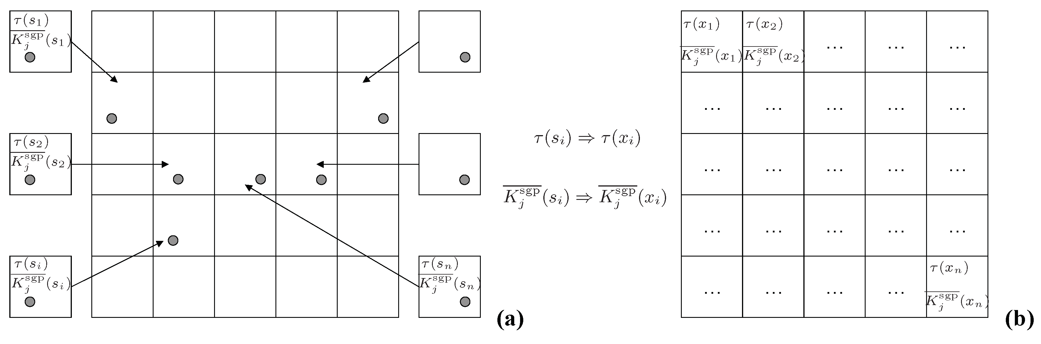
This procedure can be repeated -prior to any CTM simulation- for all small-scale simulations $s_1,s_2,\dots ,s_n$, differing for the background conditions, that generate an ensemble of $\tau$ and $\overline{K_j^{\mathrm{sgp}}}$ and $\overline{K_j^{\mathrm{sgs}}}$ (see the sketch in Figure 2a). In practice, this is equivalent to identify the computational domain of the small-scale simulations with different CTM grid-cells that are located in various regions of the globe.

3.3.2. Reconstruction of Plume Parameters

Since the plume dilution time and reaction rates are, in general, local parameters, the data-set obtained in the previous small-scale simulations has to be redistributed at each grid-cell of the CTM (see Figure 2b). This reconstruction can be done using any interpolator $\mathcal{F}$ or best-fitting technique (e.g., the least-square method):

$$\begin{array}{ccc}\hfill \tau \left(s_i\right)& \Rightarrow & \tau \left(\mathbf{x}\right)=\mathcal{F}\left\{\tau \left(s_i\right)\right\},\hfill \end{array}$$

(34)

$$\begin{array}{ccc}\hfill \overline{K_j^{\mathrm{sgp}}}\left(s_i\right)& \Rightarrow & \overline{K_j^{\mathrm{sgp}}}\left(\mathbf{x}\right)=\mathcal{F}\left\{\overline{K_j^{\mathrm{sgp}}}\left(s_i\right)\right\}\hfill \end{array}$$

(35)

where brackets indicate the ensemble of small-scale simulations. The parameters $\tau$ and $K_j^{\mathrm{sgp}}$ or $K_j^{\mathrm{sgs}}$ can be integrated in the subgrid scale models presented in Section 4 and Section 5, and the effective reaction rates can be obtained by any of Equations (30), (52) or (41).

4. Parameterization of Subgrid-Scale Processes into Large-Scale Models: Single-Scalar Formulation

The models that are described in the previous section require doubling the number of transport equations for each chemical species and parameterizing the subgrid correlations of each chemical reaction, which can be prohibitive or at least very expensive in CTM simulations. A simpler model is presented here, which is based on the concepts and the definitions introduced in the previous section. The key point is to distinguish the emitted species (e.g., ${\mathrm{NO}}_x$), $k_e=1,\dots ,N_e$ from the non-emitted species (e.g., ${\mathrm{O}}_3$), $k_{ne}=1,\dots ,N_{ne}$ (with $N_s\equiv N_e+N_{ne}$). The effects of subgrid-plume reactions are then treated in two steps: first, the concentrations of emitted species $k_e$ are diluted to background level, and then they react with the atmospheric (non-emitted) species $k_{ne}$. The overall procedure is detailed next.

4.1. Treatment of Mixing

The dynamics and mixing of atmospheric flows are generally not affected by chemistry, so that one single non-reactive scalar Z can be used to represent the transport of all chemical species in the plume:

$$\frac{\partial Z}{\partial t}+\mathsf{\nabla }·\left(Z\mathbf{u}\right)+\mathsf{\nabla }·(D\mathsf{\nabla }Z)=S_F$$

(36)

where $S_F$ is the usual fuel consumption (see Section 3.1). Applying the filter operator presented in Equation (4) to Equation (36) provides the transport equation for the grid-averaged scalar:

$$\begin{array}{c}\hfill \frac{\partial \overline{Z}}{\partial t}+\mathsf{\nabla }·\left(\overline{Z}\overline{\mathbf{u}}\right)+\mathsf{\nabla }·(D\mathsf{\nabla }\overline{Z})+\mathsf{\nabla }·(\overline{Z\mathbf{u}}-\overline{Z}\overline{\mathbf{u}})=\overline{S_F}.\end{array}$$

(37)

Using the closure defined by Equation (17) with $Z^p\equiv Z$ and $Z^a\equiv 0$ (the scalar is constructed to be zero outside the plume) yields $\mathsf{\nabla }·(\overline{Z\mathbf{u}}-\overline{Z}\overline{\mathbf{u}})=\mathsf{\nabla }·(D_{turb}\mathsf{\nabla }\overline{Z})+{\displaystyle \frac{\overline{Z}-0}{\tau }}$. Inserting the latter into Equation (37) and using Equation (21) finally yields

$${\displaystyle \frac{D\overline{Z}}{Dt}}=\overline{S_F}-{\displaystyle \frac{\overline{Z}}{\tau }}.$$

(38)

Physically, Z can be thought as a the concentration of a reservoir species that is continuously filled up through direct fuel injection ($S_F$) and continuously emptied through plume dilution ($-Z/\tau$). Its transport equation only describes the mixing process of the plume without reaction.

Instead of explicitly solving transport equations for the species in the plume, Equation (19), the plume concentration of the emitted species $\overline{C_{k_e}^p}$ is reconstructed by relating it to $\overline{Z}$ through the emission index $E{I}_{k_e}$, which is equivalent to dilute it to the scale of the grid-box:

$$\overline{C_{k_e}^p}(\mathbf{x},t)=E{I}_{k_e}\times \overline{Z}(\mathbf{x},t).$$

(39)

Note that Equation (39) neglects the reactions between emitted species inside the plume, which is a reasonable approximation in aircraft plume chemistry, like ${\mathrm{NO}}_x$/ozone chemistry. The background chemical sources $\overline{{\omega }_{k_e}^a}$ are given by Equation (28), so that the background concentrations $\overline{C_{k_e^a}}$ evolve according to

$$\begin{array}{c}\hfill {\displaystyle \frac{D\overline{C_{k_e}^a}}{Dt}}={\displaystyle \frac{E{I}_{k_e}\overline{Z}}{\tau }}+\overline{{\omega }_{k_e}^a}\end{array}$$

(40)

which formally replace the two sets of Equations (19) and (20) for emitted species $k_e$.

4.2. Treatment of Chemistry

The grid-averaged background chemical sources of non-emitted species $\overline{{\omega }_{k_{ne}}^a}$ are simply given by Equation (28). To obtain the grid-averaged plume sources $\overline{{\omega }_{k_{ne}}^p}$, it is useful to distinguish three groups of reactions: those only involving emitted species, $k_{e_j}^{\prime }\leftrightarrow k_{e_j}^{″}$; those only involving non-emitted species, $k_{n{e}_j}^{\prime }\leftrightarrow k_{n{e}_j}^{″}$; and those involving both emitted and non-emitted species, $k_{e_j}^{\prime }\leftrightarrow k_{n{e}_j}^{″}$. The first group of reactions are neglected, as already mentioned in Section 4.1, see Equation (39). The second group is also neglected, because the model assumes that concentrations of non-emitted species are diluted at the background level, $\overline{C_{k_{ne}}^p}\simeq \overline{C_{k_{ne}}^a}$, and the associated reactions are included in the the background sources $\overline{{\omega }_{k_{ne}}^a}$. Finally, the reactions of the last group are modeled in a slightly different way than in Section 3 by suitably modifying the reaction rates. Denoting, by $N_r^{e\leftrightarrow ne}$, the number of $k_{e_j}^{\prime }\leftrightarrow k_{n{e}_j}^{″}$ reactions, and using Equation (39), Equation (25) can be recast as

$$\overline{{\omega }_{k_{ne}}^p}=\sum _{j=1}^{N_r^{e\leftrightarrow ne}}\mathsf{\Delta }{\nu }_{k_{n{e}_j}}{K}_j\overline{C_{k_{e_j}^{\prime }}^p{C}_{k_{n{e}_j}^{″}}^p}=\sum _{j=1}^{N_r^{e\leftrightarrow ne}}\mathsf{\Delta }{\nu }_{k_{n{e}_j}}{K}_j^{\mathrm{eff}}\overline{C_{k_{e_j}^{\prime }}^p}\overline{C_{k_{n{e}_j}^{″}}^p}$$

(41)

where $\overline{C_{k_{e_j}^{\prime }}^p}$ is given by Equation (39), while the “effective” reaction rates $K_j^{\mathrm{eff}}$ have been introduced as

$$K_j^{\mathrm{eff}}\equiv K_j{\displaystyle \frac{\overline{C_{k_{e_j}^{\prime }}^p{C}_{k_{n{e}_j}^{″}}^p}}{\overline{C_{k_{e_j}^{\prime }}^p}\overline{C_{k_{n{e}_j}^{″}}^p}}}.$$

(42)

With all of the assumptions made above, the transport Equations (19) and (20) for the non-emitted species can be finally replaced by a single set of equations:

$${\displaystyle \frac{D\overline{C_{k_{ne}}^a}}{Dt}}=\overline{{\omega }_{k_{ne}}^a}+\sum _{j=1}^{N_r^{e\leftrightarrow ne}}\mathsf{\Delta }{\nu }_{k_{n{e}_j}}{K}_j^{\mathrm{eff}}E{I}_{k_{e_j}^{\prime }}\overline{Z}\overline{C_{k_{n{e}_j}^{″}}^a}.$$

(43)

This method has been successfully tested by [15] in a CTM in the case of aircraft ${\mathrm{NO}}_x$ emission ($N_s=5$ species and $N_r=5$ reactions), with the assumption of a constant dilution time $\tau =15$ h.

Consistency Check

Consider a plume trajectory and assume constant $S_F$ and $\tau$ to ease the analysis. Hence, Equation (38) has the approximate solution

$$\overline{Z}\left(t\right)=(Z_0-\tau S_F)e^{-t/\tau }+S_F\tau$$

(44)

where subscript 0 denotes initial conditions. In the limit of very short dilution time, $\tau \to 0$, the plume is instantaneously diluted (ID) to background, so that Equation (44) reduces to

$$\overline{Z}\simeq {\overline{Z}}_{\mathrm{ID}}=\tau S_F.$$

(45)

For emitted species, the right-hand side of Equation (40) becomes

$$E{I}_{k_e}{S}_F+\overline{{\omega }_{k_e}^a}\equiv \overline{E_{k_e}}+\overline{{\omega }_{k_e}^a}$$

(46)

which is formally the same as the right-hand side of Equation (7) written for $k=k_e$. Equations (39) and (45) also yield $\overline{C_{k_e}^p}=\tau S_{F}E{I}_{k_e}\to 0$, so that the right-hand side of Equation (43) simply becomes:

$$\overline{{\omega }_{k_{ne}}^a}\equiv \overline{{\omega }_{k_{ne}}}.$$

(47)

Thus, for very short dilution times, the instantaneous dispersion model [9] is recovered.

5. Application and Verification of the Method

In this section, a first numerical validation of the model described in Section 3 is presented. The idea is to run a fully resolved simulation over a small domain that “mimics” a single computational cell of a larger model. Considering a box of homogeneous and isotropic turbulence (HIT) and periodic boundary conditions automatically sets the large scale average transport to zero, so that $\frac{D\overline{C_k}}{Dt}=\frac{\partial \overline{C_k}}{\partial t}\equiv \frac{d\overline{C_k}}{dt}$. Thus, the species concentrations can be measured and all volume-integral (averaged) quantities can be computed exactly and compared to the model predictions. In the turbulence modeling community, this approach is often referred to as apriori testing.

The numerical code that is employed in this study to generate turbulent fluctuations is a high-resolution multi-species Navier-Stokes solver, which has been extensively used for direct numerical simulations (DNS) as well as large-eddy simulations of aircraft emissions and contrails [24,25,26]. To ensure most generality, a box of synthetic HIT is generated using a stochastic forcing technique [27] that consists in adding a body-force to the momentum equations in such a way that only the large scales (small wave-numbers) of the flow are excited. Details of the method, including the application to atmospheric clouds, can be found in Paoli and Shariff [28]. The code is written in non-dimensional form, the reference values being $L_{\mathrm{ref}}$ for length, $a_{\mathrm{ref}}$ for velocity, $t_{\mathrm{ref}}=L_{\mathrm{ref}}/a_{\mathrm{ref}}$ for time, ${\nu }_{\mathrm{ref}}$ for kinematic viscosity. A single (non-dimensional) simulation generates a set of dimensional data fields with different reference values sharing the same Reynolds number, $\mathrm{Re}=a_{\mathrm{ref}}{L}_{\mathrm{ref}}/{\nu }_{\mathrm{ref}}=2000$, Prandtl number, $\mathrm{Pr}={\mu }_{\mathrm{ref}}{C}_{p_{\mathrm{ref}}}/\lambda =0.75$, and species Schmidt number ${\mathrm{Sc}}_k={\mu }_{\mathrm{ref}}/{\rho }_{\mathrm{ref}}{D}_k=0.75$. This is useful for exploring the sensitivity of chemistry turbulence simply rescaling the reaction rates by the desired $t_{\mathrm{ref}}$, without changing the (non-dimensional) turbulent flow and the chemical reaction scheme. The low Reynolds number is due to the resolution requirements imposed by the DNS: the smallest resolved scales are of the order of the Kolmogorov dissipative length-scale. This is not a major issue here, since the objective is to numerically validate the model of effective reaction rates in the presence of generic turbulent fluctuations, and not to analyze the particular causes that drive these fluctuations. The computational domain is $L_{\mathrm{box}}^{+}=2\pi$, the box is ${64}^3$ (superscript + indicates non-dimensional variables). The flow is initially at rest, and only the body-force provides the energy to sustain turbulence. Once statistically stationary conditions are obtained (i.e., turbulent fluctuations do not grow but oscillate round steady values) the (mechanical) turnover time, defined as the ratio between the turbulent kinetic energy and the dissipation rate, is ${\tau }_e^{+}\simeq 50$ (See Paoli and Shariff [28] for detailed documentation of this DNS). Physically, this timescale is a measure of the time that is needed by viscosity to dissipate turbulent kinetic energy. In isotropic turbulence, this is also a measure of the dissipation of scalar energy by the scalar dissipation rate [20], and is then the pertinent parameter to evaluate the influence of turbulent diffusion on chemical reactions.

In particular, one can define a Damköhler number [29,30] as the ratio

$$\mathrm{Da}={\displaystyle \frac{{\tau }_e}{{\tau }_{\mathrm{ch}}}}$$

(48)

where ${\tau }_{\mathrm{ch}}$ is a characteristic timescale of the reaction and it is defined next.

The turbulence timescale ${\tau }_e$ is, in general, different from the dilution timescale $\tau$ introduced above, which is a measure of the plume lifetime. As explained in Section 3, a passive scalar equation is added to those for chemical species, and $\tau$ is defined as the time when the peak concentration of the scalar inside the plume has reduced to $1\%$ of its initial value [23,31]. In dimensionless units and for all cases that are considered here, this time is ${\tau }^{+}\simeq 175=3.5{\tau }_e^{+}$.

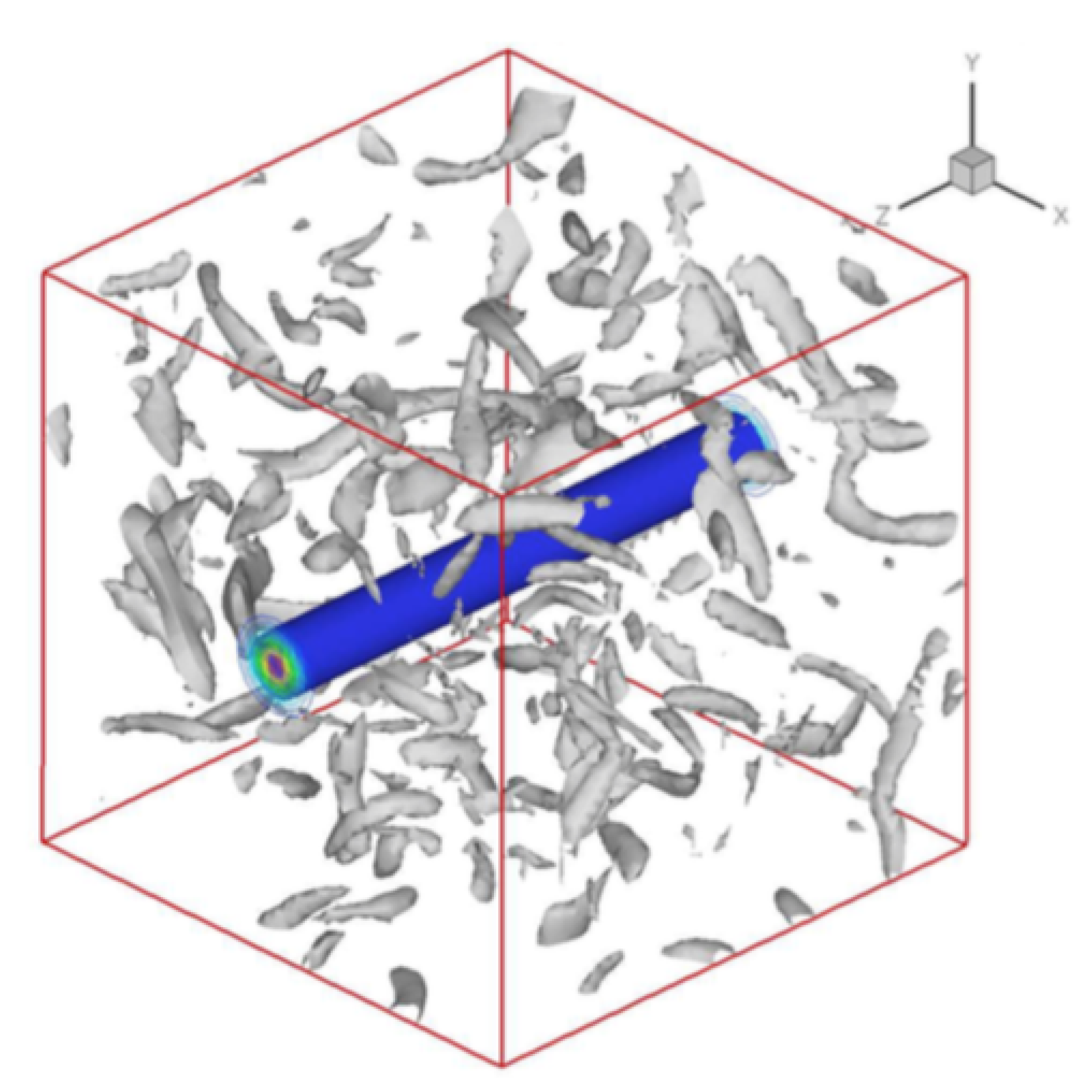
The chemical species are initialized with Gaussian distributions for the mixing ratios $X_k$ centered on the z−axis (see Figure 3):

$$X_k(0,r)=X_k^a+(X_k^p-X_k^a)exp(-r^2/{\sigma }^2)$$

(49)

where $X_k^a$ and $X_k^p$ are the background and centerline values, respectively; r is the radial distance from the centerline, and ${\sigma }^2$ is the variance of the distribution, which is chosen as $L_{\mathrm{box}}/\sigma =30$. The concentrations are then simply given by $c_k=X_k\times c_{\mathrm{air}}$, where $c_{\mathrm{air}}$ is the (constant) density of air.

An alternative derivation of the grid-averaged reaction rates is now presented, based on the subgrid correlation of concentration fluctuations rather than the explicit identification of plume and background concentrations.The idea is similar to the approach that was proposed by [29,32], and [30] among others for the simulations of turbulent reactive boundary layers. The total concentration is decomposed into grid-averaged and fluctuating terms, as:

$$\begin{array}{ccc}\hfill C_k=\overline{C_k}+C_k^{\prime }& ,& \overline{C_k^{\prime }}\equiv 0.\hfill \end{array}$$

(50)

A subgrid-scale (sgs) reaction rate may be defined as in Equation (23):

$$K_j^{\mathrm{sgs}}\equiv K_j{\displaystyle \frac{\overline{C_{k_j^{\prime }}^{\prime }{C}_{k_j^{″}}^{\prime }}}{\overline{C_{k_j^{\prime }}}\overline{C_{k_j^{″}}}}}$$

(51)

Substituting Equation (51) into Equation (23), and under the same hypotheses used above, leads to

$$\overline{{\omega }_k}=\sum _{j=1}^{N_r}\mathsf{\Delta }{\nu }_{k_j}\left(K_j+K_j^{\mathrm{sgs}}\right)\overline{C_{k_j^{\prime }}}\overline{C_{k_j^{″}}}.$$

(52)

Note that, except for the coefficient $K_j$, the definition that is given in Equation (51) is equivalent to the index of segregation introduced by [30]. It is instructive to see how the sgs fluctuations are related to plume concentrations. From Equations (10)–(14) and after some algebra one gets

$$\overline{C_{k_j^{\prime }}^{\prime }{C}_{k_j^{″}}^{\prime }}=\overline{C_{k_j^{\prime }}^a{C}_{k_j^{″}}^a}+\overline{C_{k_j^{\prime }}^p{C}_{k_j^{″}}^p}-\overline{C_{k_j^{\prime }}}\overline{C_{k_j^{″}}}\simeq \overline{C_{k_j^{\prime }}^p{C}_{k_j^{″}}^p}$$

(53)

Two sets of simulations were carried out. The first consists of an ideal three-species system and it is used for a parametric study. The second is a more realistic ${\mathrm{NO}}_x$-ozone chemistry scheme.

5.1. Ideal Chemistry

Consider three chemical species A,B and C in the box of HIT described above and reacting each other via the generic reaction

$$A+B\stackrel{K_0}{\to }C.$$

(54)

Initial conditions are specified in

Table 1. Parameters of the initial distribution of species mixing ratios of Equation (49) and initial Damköhler number for various runs while using the ideal chemistry (54).

Run	${\mathit{X}}_{\mathit{A}}^{\mathit{a}}$	${\mathit{X}}_{\mathit{A}}^{\mathit{p}}$	${\mathit{X}}_{\mathit{B}}^{\mathit{a}}$	${\mathit{X}}_{\mathit{B}}^{\mathit{p}}$	${\mathit{X}}_{\mathit{C}}^{\mathit{a}}$	${\mathit{X}}_{\mathit{C}}^{\mathit{p}}$	${\mathbf{Da}}_0$
I1	0	0.5	0.5	0	0	0	0.1
I2	0	0.5	0.5	0	0	0	1
I3	0	0.5	0.5	0	0	0	10

. Assume $c_{\mathrm{air}}=1$ and $t_{\mathrm{ref}}\equiv L_{\mathrm{ref}}/a_{\mathrm{ref}}=1$ for simplicity. According to the definitions that are given in the previous section, $c_k$ denotes the concentrations obtained from the DNS, while $C_k$ is for those predicted by the model. The corresponding evolution equations are

$$\begin{array}{c}{\displaystyle \frac{d\overline{c_{\mathrm{A}}}}{dt}}=-\left(K_0+K_0^{\mathrm{eff}}\right)\overline{c_{\mathrm{A}}}{\overline{c}}_{\mathrm{B}},\hfill \end{array}$$

(55)

$$\begin{array}{c}{\displaystyle \frac{d\overline{c_{\mathrm{B}}}}{dt}}=-\left(K_0+K_0^{\mathrm{eff}}\right)\overline{c_{\mathrm{A}}}{\overline{c}}_{\mathrm{B}},\hfill \end{array}$$

(56)

$$\begin{array}{c}{\displaystyle \frac{d\overline{c_{\mathrm{C}}}}{dt}}=+\left(K_0+K_0^{\mathrm{eff}}\right)\overline{c_{\mathrm{A}}}{\overline{c}}_{\mathrm{B}},\hfill \end{array}$$

(57)

for the DNS volume-averaged concentrations and

$$\begin{array}{c}{\displaystyle \frac{d\overline{C_{\mathrm{A}}}}{dt}}=-\left(K_0+K_0^{\mathrm{eff}}\right)\overline{C_{\mathrm{A}}}{\overline{C}}_{\mathrm{B}},\hfill \end{array}$$

(58)

$$\begin{array}{c}{\displaystyle \frac{d\overline{C_{\mathrm{B}}}}{dt}}=-\left(K_0+K_0^{\mathrm{eff}}\right)\overline{C_{\mathrm{A}}}{\overline{C}}_{\mathrm{B}},\hfill \end{array}$$

(59)

$$\begin{array}{c}{\displaystyle \frac{d\overline{C_{\mathrm{C}}}}{dt}}=+\left(K_0+K_0^{\mathrm{eff}}\right)\overline{C_{\mathrm{A}}}{\overline{C}}_{\mathrm{B}},\hfill \end{array}$$

(60)

for the model concentrations. In Equations (55)–(60), $K_0^{\mathrm{sgs}}$ is computed via either Equations (32) or (33). Note that, if Equation (32) is used, Equations (55)–(57) are exact balance equations, since they only involve instantaneous DNS data.

The characteristic chemical timescale and the Damköhler number are estimated from the (initial) plume concentration of species by

$$\begin{array}{c}{\tau }_{{\mathrm{ch}}_0}={\displaystyle \frac{\min \left(c_{\mathrm{A}}^p,c_{\mathrm{B}}^p\right)}{K_0{c}_{\mathrm{A}}^p{c}_{\mathrm{B}}^p}}={\displaystyle \frac{1}{K_0{c}_{\mathrm{A}}^p}}={\displaystyle \frac{2}{K_0}}\hfill \end{array}$$

(61)

$$\begin{array}{c}{\mathrm{Da}}_0={\displaystyle \frac{{\tau }_e}{{\tau }_{{\mathrm{ch}}_0}}}=K_0{c}_{\mathrm{A}}^p{t}_{\mathrm{ref}}{\tau }_e^{+}\simeq 25K_0\hfill \end{array}$$

(62)

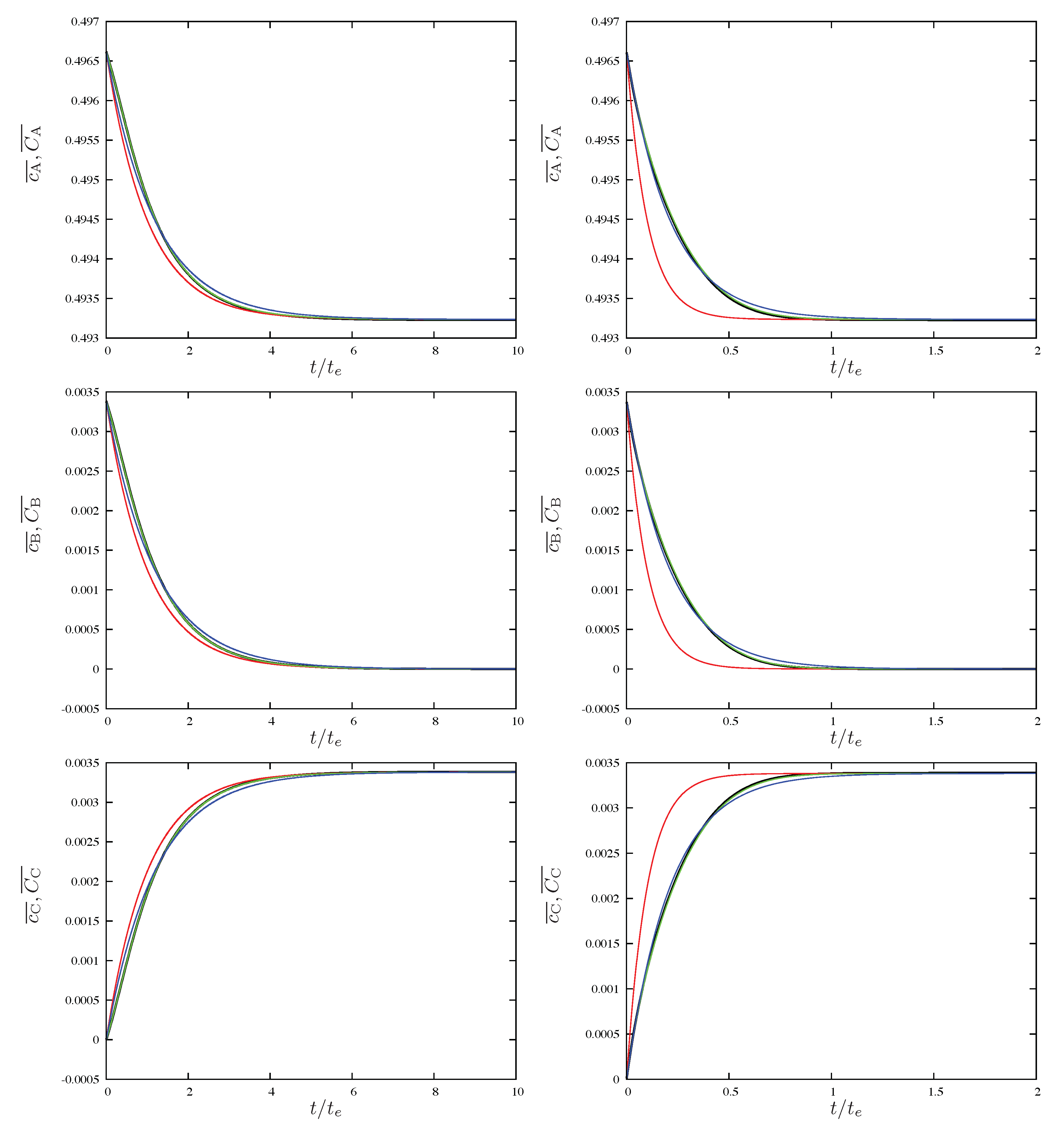
In practice, the reaction rate $K_0$ is calibrated to get the desired value of Damköhler number: three simulations when ${\mathrm{Da}}_0$ differ for one order of magnitude are performed (Table 1). Figure 4 reports the evolution of concentrations for the last two runs, I2 and I3 (respectively, with ${\mathrm{Da}}_0=1$ and 10) by comparing the “exact” evolution measured from DNS; the evolution obtained with the unmodified reaction rates, $K_0^{\mathrm{sgs}}\equiv 0$; and finally, the evolutions obtained using Equations (32) and (33) for the sgs reaction rate $K_0^{\mathrm{sgs}}$. In all cases, species A and B decrease while C increases according to (54). The curve corresponding to the accurate reconstruction of $K_0^{\mathrm{sgs}}$, Equation (32), is undistinguishable from the exact solution, which proves that the model is consistent. The figure clearly shows that both the accurate and time-average reconstruction of $K_0^{\mathrm{sgs}}$ correctly supply the subgrid-scale contribution to the overall chemical reactions: indeed, neglecting such contribution leads to overestimate the production of species C, at least for high ${\mathrm{Da}}_0$ (see Figure 4). This is also accordance with Stockwell [29] who pointed out that turbulent mixing boosts the sgs fluctuations $\overline{c_{\mathrm{A}}^{\prime }{c}_{\mathrm{B}}^{\prime }}$ and this increases with the Damköhler number.

5.2. ${\mathrm{NO}}_x$ Chemistry

This second test is closer to real cases, considering ${\mathrm{NO}}_x$-ozone chemistry in the atmosphere at the tropopause level. Five species, NO, NO₂, O, O₂, O₃, and five reactions are used:

$${\mathrm{NO}}_2\stackrel{K_1}{\to }\mathrm{NO}+\mathrm{O}$$

(63)

$$\mathrm{NO}+{\mathrm{O}}_3\stackrel{K_2}{\to }{\mathrm{NO}}_2+{\mathrm{O}}_2$$

(64)

$$\mathrm{O}+{\mathrm{O}}_2\stackrel{K_3}{\to }{\mathrm{O}}_3$$

(65)

$$\mathrm{O}+{\mathrm{NO}}_2\stackrel{K_4}{\to }\mathrm{NO}+{\mathrm{O}}_2$$

(66)

$$\mathrm{O}+{\mathrm{O}}_3\stackrel{K_5}{\to }2{\mathrm{O}}_2$$

(67)

with the corresponding reaction rates given by [33]:

$$\begin{array}{c}{K}_1=8.7\times {10}^{-3},\hfill \end{array}$$

(68)

$$\begin{array}{c}{K}_2=2\times {10}^{-12}exp\left(-1400/T_{\mathrm{air}}\right),\hfill \end{array}$$

(69)

$$\begin{array}{c}{K}_3=c_{\mathrm{air}}\times 6\times {10}^{-34}exp\left(-1400/T_{\mathrm{air}}\right),\hfill \end{array}$$

(70)

$$\begin{array}{c}{K}_4=6.5\times {10}^{-12}exp\left(120/T_{\mathrm{air}}\right),\hfill \end{array}$$

(71)

$$\begin{array}{c}{K}_5=8\times {10}^{-2}exp\left(-2050/T_{\mathrm{air}}\right).\hfill \end{array}$$

(72)

Temperature and concentration of air, $T_{\mathrm{air}}=220\mathrm{K}$, $c_{\mathrm{air}}=7.8\times {10}^{18}{\mathrm{cm}}^{-3}$, and the background mixing ratios $X_k^a$ are taken as typical values that are encountered at flight level of 11 Km, while the plume mixing ratios $X_p$ are taken from Garnier et al. [34] and are representative of emissions in the near-field of an aircraft wake. To evaluate the impact of turbulence fluctuations, three runs were carried out (labeled in

Table 2. Parameters of the initial distribution of species mixing ratios of Equation (49) and initial Damköler number for various runs and the simplified ${\mathrm{NO}}_x$ chemistry (63)–(67).

Run	${\mathit{X}}_{\mathbf{NO}}^{\mathit{a}}$	${\mathit{X}}_{\mathbf{NO}}^{\mathit{p}}$	${\mathit{X}}_{{\mathrm{NO}}_2}^{\mathit{a}}$	${\mathit{X}}_{{\mathrm{NO}}_2}^{\mathit{p}}$	${\mathit{X}}_{\mathbf{O}}^{\mathit{a}}$	${\mathit{X}}_{\mathbf{O}}^{\mathit{p}}$	${\mathit{X}}_{{\mathbf{O}}_2}^{\mathit{p}}$	${\mathit{X}}_{{\mathbf{O}}_2}^{\mathit{p}}$	${\mathit{X}}_{{\mathbf{O}}_3}^{\mathit{p}}$	${\mathit{X}}_{{\mathbf{O}}_3}^{\mathit{p}}$	${\mathbf{Da}}_2$
N1	$6\times {10}^{-12}$	${10}^{-5}$	$2\times {10}^{-12}$	${10}^{-6}$	0	0	$0.2$	$0.2$	$2\times {10}^{-7}$	$2\times {10}^{-7}$	4.2
N2	$6\times {10}^{-12}$	${10}^{-5}$	$2\times {10}^{-12}$	${10}^{-6}$	0	0	$0.2$	$0.2$	$2\times {10}^{-7}$	$2\times {10}^{-7}$	8.4
N3	$6\times {10}^{-12}$	${10}^{-5}$	$2\times {10}^{-12}$	${10}^{-6}$	0	0	$0.2$	$0.2$	$2\times {10}^{-7}$	$2\times {10}^{-7}$	13.5

with N1, N2, and N3) that differ by the value of the reference time $t_{\mathrm{ref}}$ (used to non-dimensionalize the chemical reaction rates) and by the Damköhler number calculated as in Equation (78). Note that changing $t_{\mathrm{ref}}$ is equivalent to rescaling the dimensions of the computational domain for fixed velocity fluctuations. Following the same conventions, the evolution equations of $\begin{array}{c}\hfill \mathrm{NO}\end{array}$ and ozone volume-averaged DNS concentrations $\overline{c_k}$ are

$$\begin{array}{ccc}\hfill {\displaystyle \frac{d\overline{{\mathrm{c}}_{\mathrm{NO}}}}{dt}}& =& K_1\overline{{\mathrm{c}}_{\mathrm{NO}}}-\left(K_2+K_2^{\mathrm{sgs}}\right)\overline{{\mathrm{c}}_{\mathrm{NO}}}\overline{{\mathrm{c}}_{{\mathrm{O}}_3}}-\left(K_4+K_4^{\mathrm{sgs}}\right)\overline{{\mathrm{c}}_{\mathrm{O}}}\overline{{\mathrm{c}}_{{\mathrm{NO}}_2}}\hfill \end{array}$$

(73)

$$\begin{array}{ccc}\hfill {\displaystyle \frac{d\overline{{\mathrm{c}}_{{\mathrm{O}}_3}}}{dt}}& =& -\left(K_2+K_2^{\mathrm{sgs}}\right)\overline{{\mathrm{c}}_{\mathrm{NO}}}\overline{{\mathrm{c}}_{{\mathrm{O}}_3}}-\left(K_3+K_3^{\mathrm{sgs}}\right)\overline{{\mathrm{c}}_{\mathrm{O}}}\overline{{\mathrm{c}}_{{\mathrm{O}}_2}}-\left(K_5+K_5^{\mathrm{sgs}}\right)\overline{{\mathrm{c}}_{\mathrm{O}}}\overline{{\mathrm{c}}_{{\mathrm{O}}_3}}\hfill \end{array}$$

(74)

while for the model concentrations $\overline{C_k}$ they are:

$$\begin{array}{ccc}\hfill {\displaystyle \frac{d\overline{{\mathrm{C}}_{\mathrm{NO}}}}{dt}}& =& K_1\overline{{\mathrm{C}}_{\mathrm{NO}}}-\left(K_2+K_2^{\mathrm{sgs}}\right)\overline{{\mathrm{C}}_{\mathrm{NO}}}\overline{{\mathrm{C}}_{{\mathrm{O}}_3}}-\left(K_4+K_4^{\mathrm{sgs}}\right)\overline{{\mathrm{C}}_{\mathrm{O}}}\overline{{\mathrm{C}}_{{\mathrm{NO}}_2}}\hfill \end{array}$$

(75)

$$\begin{array}{ccc}\hfill {\displaystyle \frac{d\overline{{\mathrm{C}}_{{\mathrm{O}}_3}}}{dt}}& =& -\left(K_2+K_2^{\mathrm{sgs}}\right)\overline{{\mathrm{C}}_{\mathrm{NO}}}\overline{{\mathrm{C}}_{{\mathrm{O}}_3}}-\left(K_3+K_3^{\mathrm{sgs}}\right)\overline{{\mathrm{C}}_{\mathrm{O}}}\overline{{\mathrm{C}}_{{\mathrm{O}}_2}}-\left(K_5+K_5^{\mathrm{sgs}}\right)\overline{{\mathrm{C}}_{\mathrm{O}}}\overline{{\mathrm{C}}_{{\mathrm{O}}_3}}\hfill \end{array}$$

(76)

The relevant reaction for the environmental impact is (64), i.e., the destruction of ozone by $\mathrm{NO}$. The timescale associated to this reaction is

$$\begin{array}{c}{\tau }_{{\mathrm{ch}}_2}={\displaystyle \frac{\min \left(c_{\mathrm{NO}}^p,c_{{\mathrm{O}}_3}^p\right)}{K_2{c}_{\mathrm{NO}}^p{c}_{{\mathrm{O}}_3}^p}}={\displaystyle \frac{1}{K_2{c}_{\mathrm{NO}}^p}}\simeq 3.7\mathrm{s}.\hfill \end{array}$$

(77)

$$\begin{array}{c}{\mathrm{Da}}_2\equiv {\displaystyle \frac{{\tau }_e}{{\tau }_{{\mathrm{ch}}_2}}}=K_2{c}_{\mathrm{NO}}^p{t}_{\mathrm{ref}}{\tau }_e^{+}\simeq 13.5t_{\mathrm{ref}}.\hfill \end{array}$$

(78)

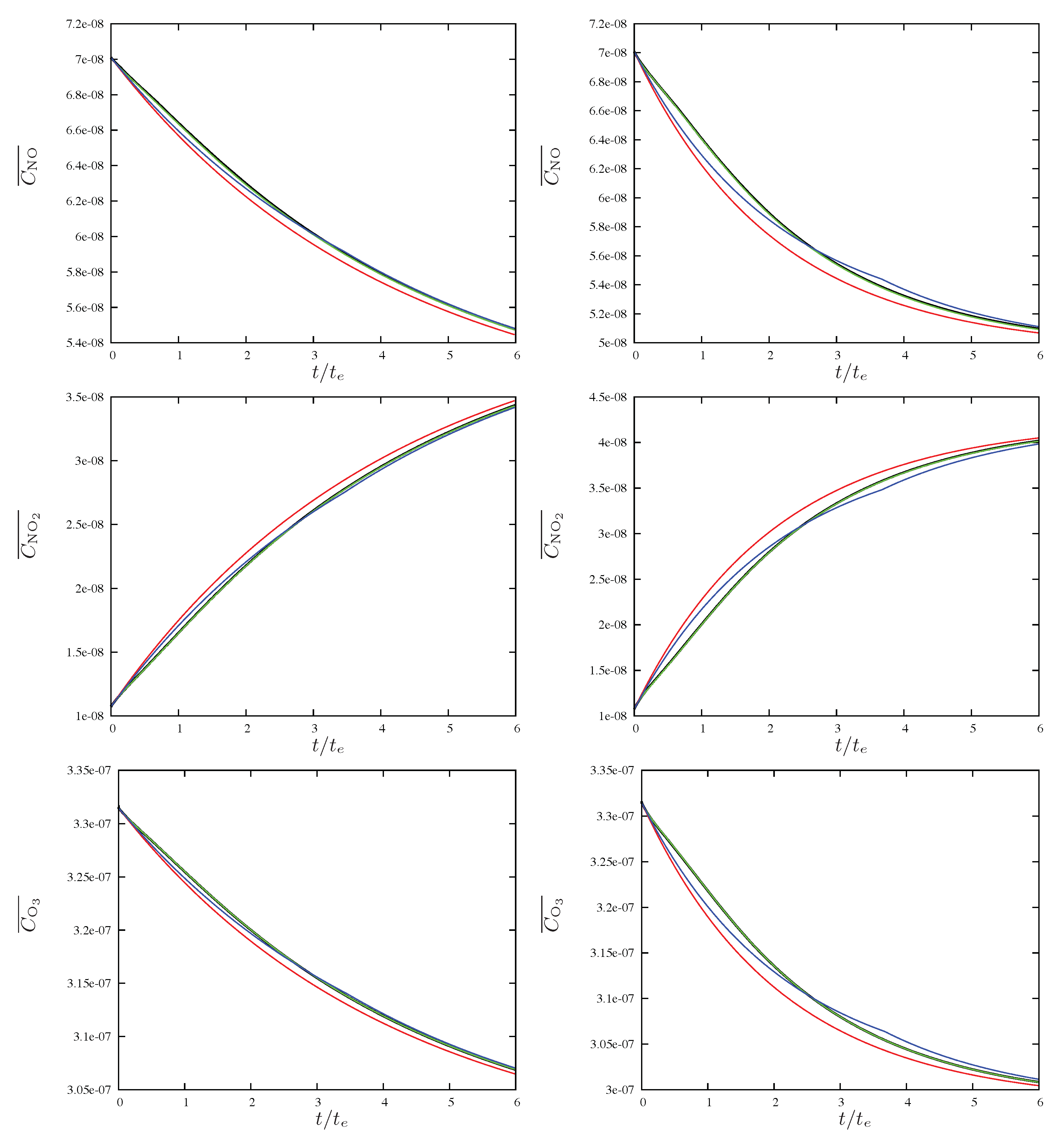
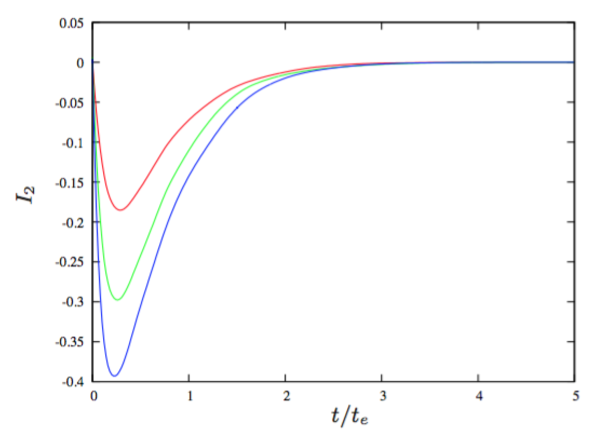
Figure 5 shows the evolution of ${\mathrm{NO}}_x$ and $\begin{array}{c}\hfill O3\end{array}$ for cases N1 and N2, when comparing the same set of curves as in the case of ideal chemistry. The effect of subgrid-scale chemistry increases with ${\mathrm{Da}}_2$. Furthermore, when the accurate reconstruction, Equation (32), is used for the sgs reaction $K_2^{\mathrm{sgs}}$, the exact DNS evolution of the concentrations is recovered. When the time-average reconstruction, Equation (33), is used as sgs model, the estimation of the concentrations is still improved compared to the standard “no-model” case, up to approximately the plume lifetime, $t=\tau \simeq 3.5t_e$. After this time, the reaction rate has to be reset to the background value, $K_j^{\mathrm{sgs}}=K_j$, because the model assumes that all species are diluted at background level. The difference between the model results and the DNS data is due to the approximation in the reconstruction of $K_j^{\mathrm{sgs}}$: in fact, in this case, the model provides the time-averaged sgs reaction rate rather than the instantaneous reaction rate. This point is further clarified in Figure 6, where the evolution of the index of segregation of reaction (64) [30] is reported as $I_2=K_2^{\mathrm{sgs}}/K_2$. The figure shows that segregation of $\begin{array}{c}\hfill \mathrm{NO}\end{array}$ and ozone initially decreases, which reflects the efficiency of the reaction is reduced; it reaches a peak value (about 0.4 for run N3) at $t=t_{\mathrm{peak}}\simeq 0.25t_e$, and finally decreases when the plume and background species get sufficiently well mixed. Therefore, the use of Equation (33) is equivalent to smooth out the segregation over the lifetime of the plumes, since it approximates the curve in Figure 6 by its integral. Even though the subgrid plume effects on the (average) species concentrations amount to a few percents at the end of the simulation in this idealized case, these values can be much higher in real atmospheric simulations where plume concentrations are initially higher, the plume may not diffusion as fast and/or is impacted by large-scale winds or other processes. This can be qualitatively appreciated by looking again at Figure 6: if these processes occur over time scales during which the segregation index is high (up to 40% as in the HIT example), the effects of subgrid plume will be considerably higher and will cumulatively impact the evolution of species concentrations much more vigorously than a simple diffusion of an HIT. From a CTM perspective, this was indeed observed in the applications of the ERR method—that corresponds to the simplified, single scalar version of the current model–[15,16]: those studies showed that when the ERR are activated, ozone depletion by ${\mathrm{NO}}_{\mathrm{x}}$ emissions from aircraft and ships was reduced by 20 to 30% along flight corridors and ship routes, respectively, as compared to the standard, instantaneous dilution approach.

One natural improvement of Equation (33) consists in using time-dependent parameterizations that fit the exact reconstruction of Equation (32). However, accurate plume dilution laws can rapidly become very complicated, depending on the flow characteristics (as shown, for example, by [35] in the case of ship-plume emissions in a boundary layer), so that the resulting parameterization could again be too expensive to implement in CTM. A simpler approach is to introduce multiple dilution timescales for each particular regime of the sgs reactions (for example, in the present case, one timescale ${\tau }_1$ for the growing regime of segregation, $t<t_{\mathrm{peak}}$, and another timescale ${\tau }_2$ for the falling regime $t_{\mathrm{peak}}<t<\tau$). The application and testing of such improvements to atmospheric chemical reactions is left for future work.

6. Discussions and Conclusions

Emissions from localized sources, such as aircraft or ship engines, evolve into small-scale plumes that are to expensive to be explicitly solved by CTM, but need to be modeled at subgrid-scale level. In principle, the physical and chemical processes occurring in the plumes and their interactions with the atmosphere can be accounted for by solving dedicated conservation equations for plume and background concentrations for each chemical species.

This study addressed this issue by deriving these sets of equations starting from the general conservation laws of species in a fluid and proposed a method to incorporate emissions from localized sources into CTM. In particular, the unknown chemical sources in the plume can be parameterized by modifying the original large-scale reaction rates while using available data from small-scale plume simulations. In a simpler version of this method, which corresponds to the ERR parameterization proposed in the past [8,15], the transport equation of only one scalar is needed. In this case, the concentrations of the emitted species in the plume can be reconstructed by diluting the emission to the size of the CTM grid-cell, while the modified reaction rates are used to model reactions with the non-emitted species.

Regardless of the choice of the parameterization (ERR, ECF, or EEI methods), verification is an important step to assess the mathematical and physical consistency of the model and is indeed customary in many areas of geophysical or engineering sciences (see, e.g., [36]). Generally speaking, verification is the process of determining whether the model works in a specific implementation it has been designed for, whereas validation is the process of determining whether the model gives a good representation of real world. This distinction is particularly crucial to test plume parameterizations in CTM, because only verification is the only means to identify the error intrinsic to the parameterizations from the errors/inaccuracies of the CTM itself. The practical implementation of verification techniques depends on specific situations but as a general rule, one can borrow ideas from other areas, such as in the turbulence modeling community (where it is often called a posteriori testing). An instructive exercise of verification consists in setting up an ideal scenario where a plume is initialized into a large computational domain (with sufficient resolution for the plume to be explicitly resolved). Species concentrations in such domain evolve according to some model equations (that we may call global model) without any subgrid treatment of the plume. In this ideal situation and assuming the global model is exact, the model output is also exact. Subsequently, the same model can be run again on the same domain using much lower resolution so that the plume is not explicitly resolved (as in a real CTM), but activating the subgrid parameterizations (EEI, ECF, or ERR). The volume-averaged species concentrations obtained from the latter run should then match or be close to the exact model output of the first run. Again, this exercise can only guarantee that the parameterization reproduces the correct large-scale behavior of the full model under identical conditions. In the present study, this has been verified for the ERR case in the ideal scenario of a reactive plume evolving in homogenous turbulence using Direct Numerical Simulations. Interesting follow-up studies would be to extend the verification analysis of the subgrid model in more complex plume configurations, such as, for example, a plume subject to background turbulence with differential diffusion along the three directions and/or to three-dimensional shear in the form of a prescribed large-scale velocity gradient [9]. The final goal is of the integration of the subgrid plume into CTM, on the line of the experiments conducted using the ERR method [15]. Even though the method presented here is sufficiently general to be applied to each of the chemical reaction rates of a CTM using for example Equations (32) or (33), in practice the subgrid plume parameterization could be activated, in a first step, only for the most relevant reactions based on previous knowledge of the chemical system. This is indeed left to future work.

References

- Paoli, R.; Shariff, K. Contrail modeling and simulation. Annu. Rev. Fluid Mech. 2016, 48, 393–427. [Google Scholar] [CrossRef] [Green Version]
- Paoli, R.; Thouron, O.; Cariolle, D.; Garcia, M.; Escobar, J. Three-dimensional large-eddy simulations of the early phase of contrail-to-cirrus transition: Effects of atmospheric turbulence and radiative transfer. Meteorol. Z. 2017, 26, 597–620. [Google Scholar] [CrossRef]
- Song, C.H.; Chen, G.; Hanna, S.R.; Crawford, J.; Davis, D.D. Dispersion and chemical evolution of ship plumes in the marine boundary layer: Investigation of O3/NOx/HOx chemistry. J. Geophys. Res. 2003, 108, 4143. [Google Scholar] [CrossRef]
- Brasseur, G.P.; Müller, J.F.; Granier, C. Atmospheric impact of NOx emissions by subsonic aircraft. J. Geophys. Res. 1996, 101, 1423–1428. [Google Scholar] [CrossRef]
- Meijer, E.W.; van Velthoven, P.F.J.; Wauben, W.M.F.; Beck, J.P.; Velders, G.J.M. The effect of the conversion of the nitrogen oxides in aircraft exhaust plumes in global models. Geophys. Res. Lett. 1997, 24, 3013–3016. [Google Scholar] [CrossRef]
- Kraabøl, A.G.; Flatøy, F.; Stordal, F. Impact of NOx emissions from subsonic aircraft: Inclusion of plume processes in a three-dimensional modeling covering Europe, North America and North Atlantic. J. Geophys. Res. 2000, 105, 3573–3582. [Google Scholar] [CrossRef]
- Kraabøl, A.G.; Berntsen, T.K.; Sundet, J.K.; Stordal, F. Impacts of NOx emissions from subsonic aircraft in a global three-dimensional chemistry transport model including plume processes. J. Geophys. Res. 2002, 107, 4655–4667. [Google Scholar] [CrossRef]
- Paoli, R.; Cariolle, D.; Sausen, R. Review of effective emissions modeling and computation. Geosci. Model Dev. 2011, 4, 643–677. [Google Scholar] [CrossRef] [Green Version]
- Petry, H.; Hendricks, J.; Möllhoff, M.; Lippert, E.; Meier, A.; Sausen, R. Chemical conversion of subsonic aircraft emissions in the dispersing plume: Calculation of effective emission indices. J. Geophy. Res. 1998, 103, 5759–5772. [Google Scholar] [CrossRef]
- Meijer, E.W. Modeling the Impact of Subsonic Aviation on the Composition of the Atmosphere. Ph.D. Thesis, Technische Universiteit Eindhoven, Eindhoven, The Netherlands, 2001. [Google Scholar]
- Kraabøl, A.G.; Konopka, P.; Stordal, F.; Schlager, H. Modelling chemistry in aircraft plumes 1: Comparison with observations and evaluation of a layered approach. Atmos. Environ. 2000, 34, 3939–3950. [Google Scholar] [CrossRef] [Green Version]
- Kraabøl, A.G.; Stordal, F. Modelling chemistry in aircraft plumes 2: The chemical conversion of NOx to reservoir species under different conditions. Atmos. Environ. 2000, 34, 3951–3962. [Google Scholar] [CrossRef]
- Karol, I.; Ozolin, Y.E.; Kiselev, A.A.; Rozanov, E.V. Plume Transformation Index (PTI) of the subsonic aircraft exhausts and their dependence on the external conditions. Geophys. Res. Lett. 2000, 27, 373–376. [Google Scholar] [CrossRef]
- Meilinger, S.K.; Ka¨rcher, B.; Peter, T. Microphysics and heterogeneous chemistry in aircraft plumes-high sensitivity on local meteorology and atmospheric composition. Atmos. Chem. Phys. 2005, 5, 533–545. [Google Scholar] [CrossRef] [Green Version]
- Cariolle, D.; Caro, D.; Paoli, R.; Hauglustaine, D.; Cuenot, B.; Cozic, A.; Paugam, R. Parameterization of plume chemistry into large scale atmospheric models: Application to aircraft NOx emissions. J. Geophys. Res. 2009, 114, D19302. [Google Scholar] [CrossRef]
- Huszar, P.; Cariolle, D.; Paoli, R.; Halenka, T.; Belda, M.; Schlager, H.; Miksovsky, J.; Pisoft, P. Modeling the regional impact of ship emissions on NOx and ozone levels over the Eastern Atlantic and Western Europe using ship plume parameterization. Atmos. Chem. Phys. 2010, 10, 6645–6660. [Google Scholar] [CrossRef] [Green Version]
- Gressent, A.; Sauvage, B.; Cariolle, D.; Evans, M.; Leriche, M.; Mari, C.; Thouret, V. Modeling lightning-NOx chemistry on a sub-grid scale in a global chemic al transport model. Atmos. Chem. Phys. 2016, 16, 5867–5889. [Google Scholar] [CrossRef] [Green Version]
- Seigneur, C.; Tesche, T.W.; Roth, P.M.; Liu, M.K. On the treatment of point source emissions in urban air quality modeling. Atmos. Environ. 1983, 17, 1655–1676. [Google Scholar] [CrossRef]
- Karamchandani, P.; Santos, L.; Sykes, I.; Zhang, Y.; Tonne, C.; Seigneur, C. Development and Evaluation of a State-of-the-Science Reactive Plume Model. Environ. Sci. Technol. 2000, 34, 870–880. [Google Scholar] [CrossRef]
- Pope, S.B. Turbulent Flows; Cambridge University Press: Cambridge, UK, 2000. [Google Scholar]
- Villermaux, J.; Devillon, J.C. Représentation de la coalescence et de la redispersion des domaines de ségrégation dans un fluide par un modèle d’interaction phénoménologique. In Proceedings of the Second International Symposium on Chemical Reaction Engineering, Amsterdam, The Netherlands, 2–4 May 1972. [Google Scholar]
- Dopazo, C.; O’Brien, E.E. An approach to the autoignition of a turbulent mixture. Acta Astronaut. 1974, 1, 1239–1266. [Google Scholar] [CrossRef]
- Schlager, H.; Konopka, P.; Schulte, P.; Schumann, U.; Ziereis, H.; Arnold, F.; Klemm, M.; Hagen, D.; Whitefield, P.; Ovarlez, J. In situ observations of air traffic emission signatures in the North Atlantic flight corridor. J. Geophys. Res. 1997, 102, 10739–10750. [Google Scholar] [CrossRef] [Green Version]
- Paoli, R.; Hélie, J.; Poinsot, T. Contrail formation in aircraft wakes. J. Fluid Mech. 2004, 502, 361–373. [Google Scholar] [CrossRef] [Green Version]
- Paoli, R.; Vancassel, X.; Garnier, F.; Mirabel, P. Large-eddy simulation of a turbulent jet and a vortex sheet interaction: Particle formation and evolution in the near-field of an aircraft wake. Meteorol. Z. 2008, 17, 131–144. [Google Scholar] [CrossRef]
- Paoli, R.; Nybelen, L.; Picot, J.; Cariolle, D. Effects of jet/vortex interaction on contrail formation in supersaturated conditions. Phys. Fluids 2013, 25, 053305. [Google Scholar] [CrossRef]
- Eswaran, V.; Pope, S.B. An examination of forcing in direct numerical simulations of turbulence. Comput. Fluids 1988, 16, 257–278. [Google Scholar] [CrossRef]
- Paoli, R.; Shariff, K. Turbulent condensation of droplets: Direct simulation and a stochastic model. J. Atmos. Sci. 2009, 66, 723–740. [Google Scholar] [CrossRef]
- Stockwell, W.R. Effects of turbulence on gas-phase atmospheric chemistry: Calculation of the relationship between time scales for diffusion and chemical reactions. Meteorol. Atmos. Phys. 1995, 57, 159–171. [Google Scholar] [CrossRef]
- Vilà-Guerau de Arellano, J.; Dosio, A.; Vinuesa, J.F.; Holtsag, A.A.M.; Galmarini, S. The dispersion of chemically reactive species in the atmospheric boundary layer. Meteorol. Atmos. Phys. 2004, 87, 23–28. [Google Scholar] [CrossRef]
- Gerz, T.; Dürbeck, T.; Konopka, P. Transport and effective diffusion of aircraft emissions. J. Geophys. Res. 1998, 103, 25905–25914. [Google Scholar] [CrossRef] [Green Version]
- Schumann, U. Large-eddy simulation of turbulent diffusion with chemical reactions in the convective boundary layer. Atmos. Environ. 1989, 23, 1713–1729. [Google Scholar] [CrossRef] [Green Version]
- Sander, S.P.; Friedl, R.R.; Golden, D.M.; Kurylo, M.J.; Moortgat, G.K.; Keller-Rudek, H.; Wine, P.H.; Ravishankara, A.R.; Kolb, C.E.; Molina, M.J.; et al. Chemical Kinetics and Photochemical Data for Use in Atmospheric Studies: Evalutaion Number 15; Tec. Rep. Publ. 06-2; JPL, NASA: Pasadena, CA, USA, 2006. [Google Scholar]
- Garnier, F.; Baudoin, C.; Woods, P.; Louisnard, N. Engine Emission alteration in the near field of an aircraft. Atmos. Environ. 1997, 31, 1767–1781. [Google Scholar] [CrossRef]
- Chosson, F.; Paoli, R.; Cuenot, B. Ship plume dispersion rates in convective boundary layers for chemistry models. Atmos. Chem. Phys. 2008, 8, 4841–4853. [Google Scholar] [CrossRef] [Green Version]
- Roache, P.J. Verification and Validation in Computational Science and Engineering; Hermosa Publishers: Albuquerque, NM, USA, 1998. [Google Scholar]
Figure 1.
Sketch of a cut of a plume of volume inside a CTM cell of volume V centered at : and are the concentrations of a species k according to Equation (10).
Figure 2.
Sketch of the method used to compute the grid-average plume reaction rates : (a) an ensemble of small-scale plume simulations is run by changing the local background conditions that are representative of the CTM grid-cells. The resulting small-scale concentrations are used to get and while using Equations (29) or (42) for each ; (b) the plume reaction rates are then reconstructed at each grid-point of the CTM by interpolating/best-fitting the pre-computed rates by means of Equations (34) and (35). The procedure is exactly the same for the subgrid-scale reaction rates and .
Figure 3.
Arbitrary iso-surfaces of the initial species concentration (blue) in the statistically stationary turbulence (light gray). The contour lines represent the scaled concentration in Equation (49).
Figure 4.
Evolution of computed and model grid-averaged species concentrations for run I1 (left panel) and I2 (right panel). ![Atmosphere 11 00863 i001]() : DNS data;
: DNS data; ![Atmosphere 11 00863 i002]() : no model;
: no model; ![Atmosphere 11 00863 i003]() : model prediction, Equation (32);
: model prediction, Equation (32); ![Atmosphere 11 00863 i004]() : model prediction, Equation (33).
: model prediction, Equation (33).
: DNS data;
: no model;
: model prediction, Equation (32);
Figure 5.
Evolution of computed and predictedcgrid-averaged species concentrations forcrun N1 (left panels, ) and N2 (right panels, ).c ![Atmosphere 11 00863 i001]() : DNS data;
: DNS data; : no model; : model prediction, Equation (32); : model prediction, Equation (33).
Figure 6.
Time evolution of the index of segregation of reaction (64), extracted from DNS data. ![Atmosphere 11 00863 i002]() : run N1 ();
: run N1 (); ![Atmosphere 11 00863 i003]() : run N2 ();
: run N2 (); ![Atmosphere 11 00863 i004]() : run N3 ().
: run N3 ().
: run N1 (); : run N2 (); : run N3 ().