
Detecting High-Resolution Adversarial Images with Few-Shot Deep Learning


Abstract
:1. Introduction
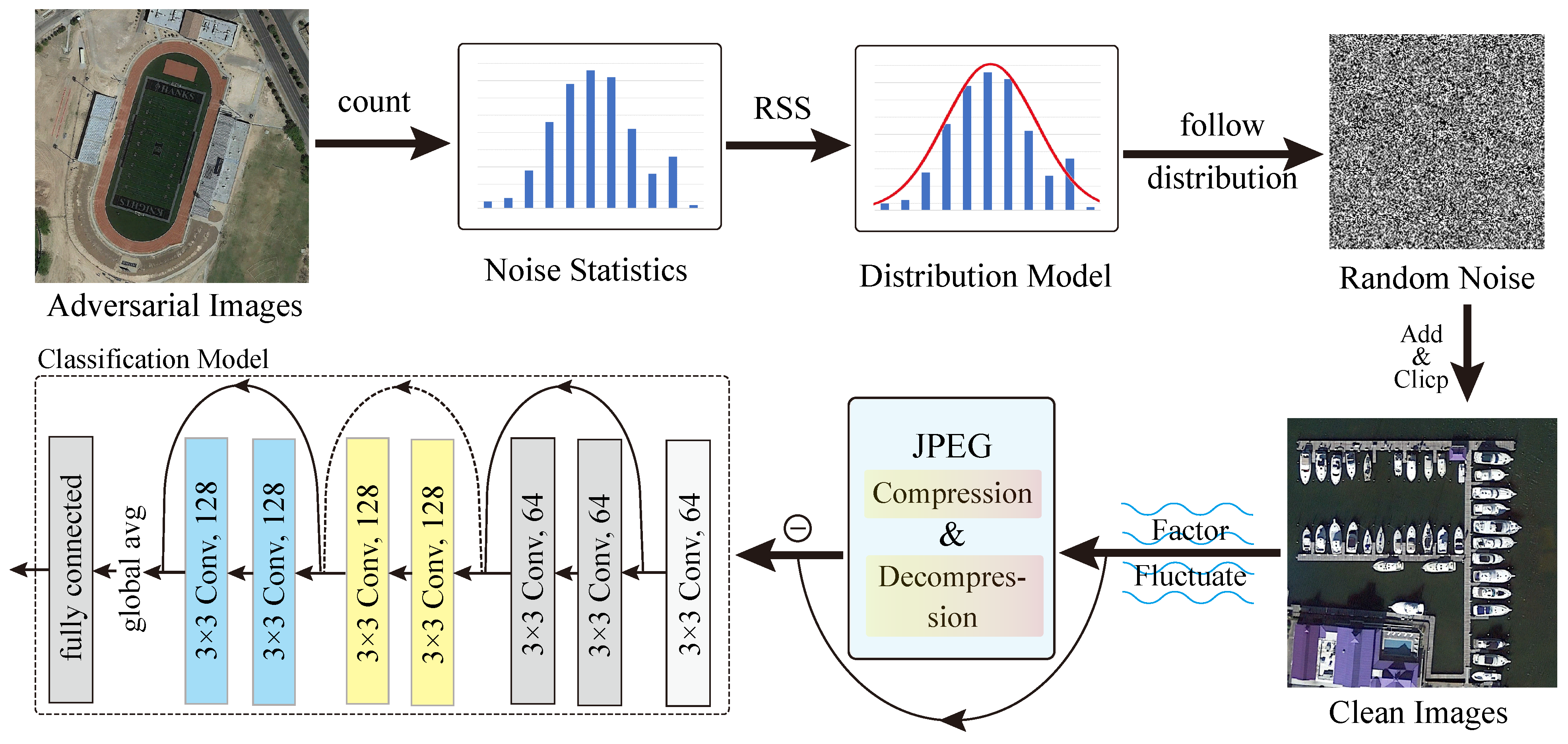
- Pseudoadversarial examples are generated through simulation to train the detector so that the training model no longer requires many real adversarial examples. A small amount of real adversarial noise is used to fit the distribution, and pseudoadversarial examples are generated based on this distribution;
- A dynamic simulation training strategy for the entire detector training process is proposed based on pseudoadversarial examples. With the cooperation of a small number of real examples, JPEG error input, and compression factor fluctuation, the dynamic simulation training strategy helps common classification models to detect adversarial examples;
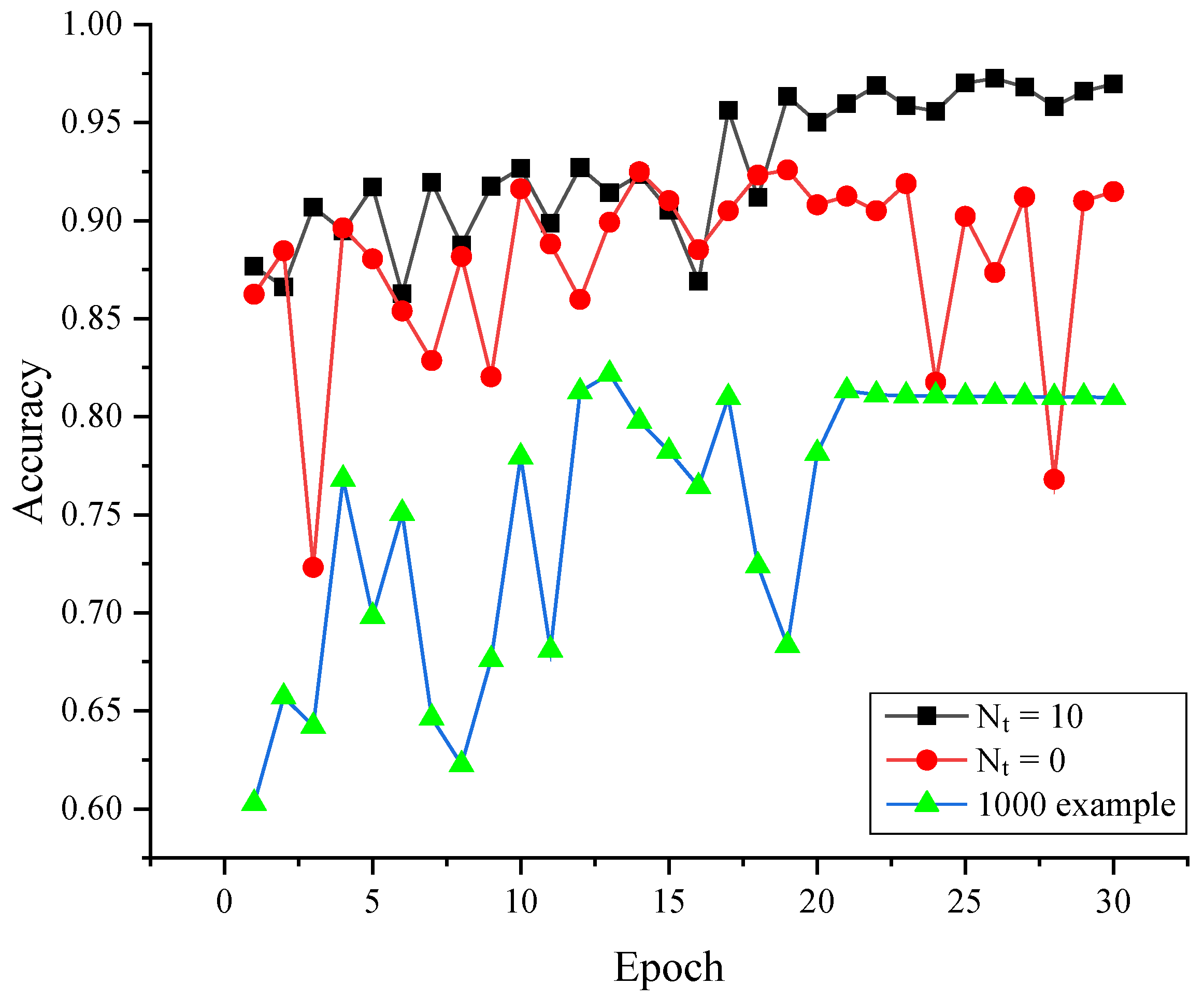
- Because pseudoadversarial examples are generated in real time during the training process of the detection model and the noise generated in each epoch is different, the serious overfitting phenomenon is avoided. Benefiting from this, the common classification model performs well in adversarial example detection.
2. Related Works
2.1. Adversarial Example Generation
2.2. Defense of Adversarial Examples
3. Prior Knowledge
3.1. JPEG Encoding and Decoding
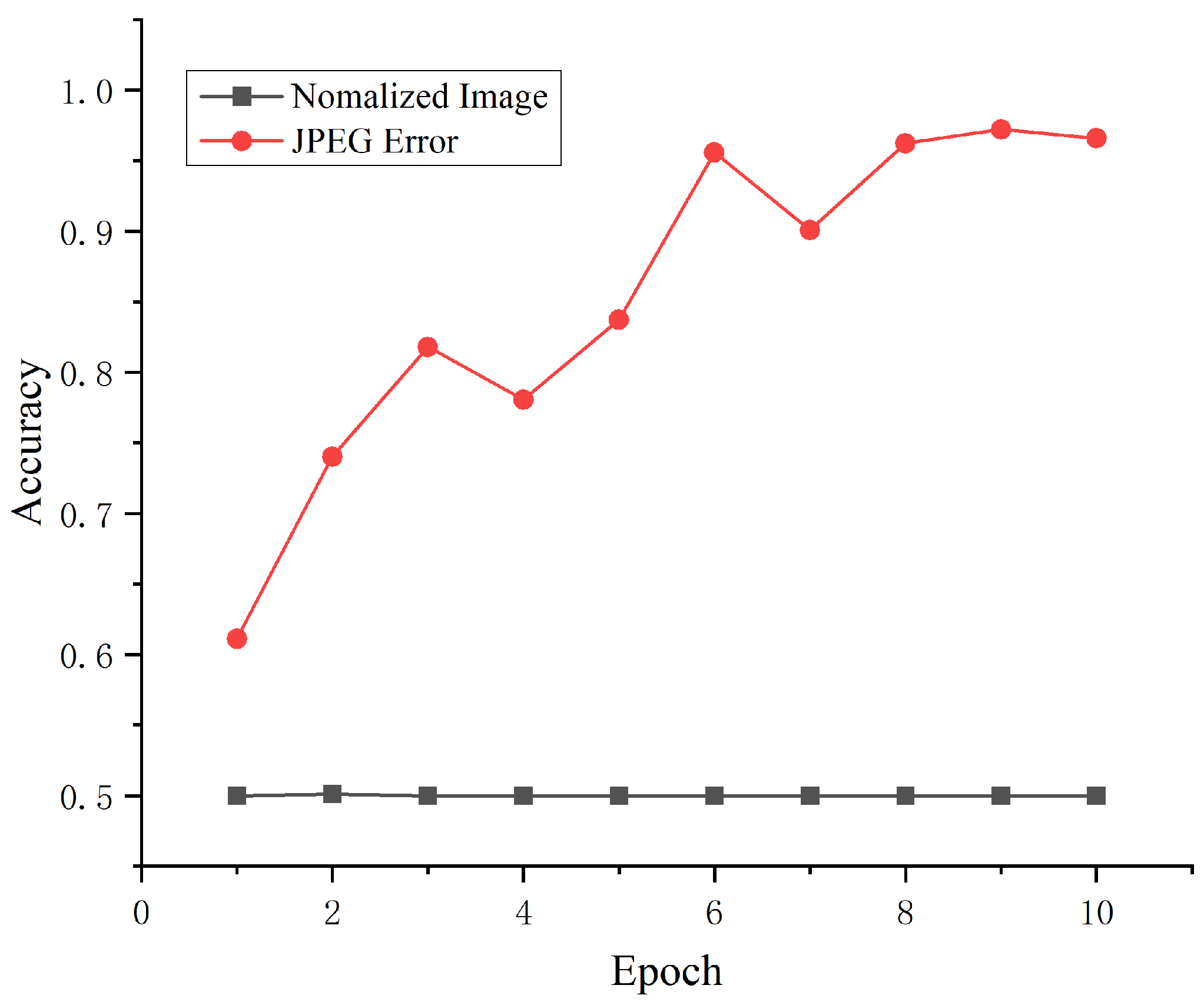
3.2. JPEG Error and Adversarial Example Detection
4. Dynamic Simulation Training Strategy
4.1. Problem Description
4.2. Overall Process
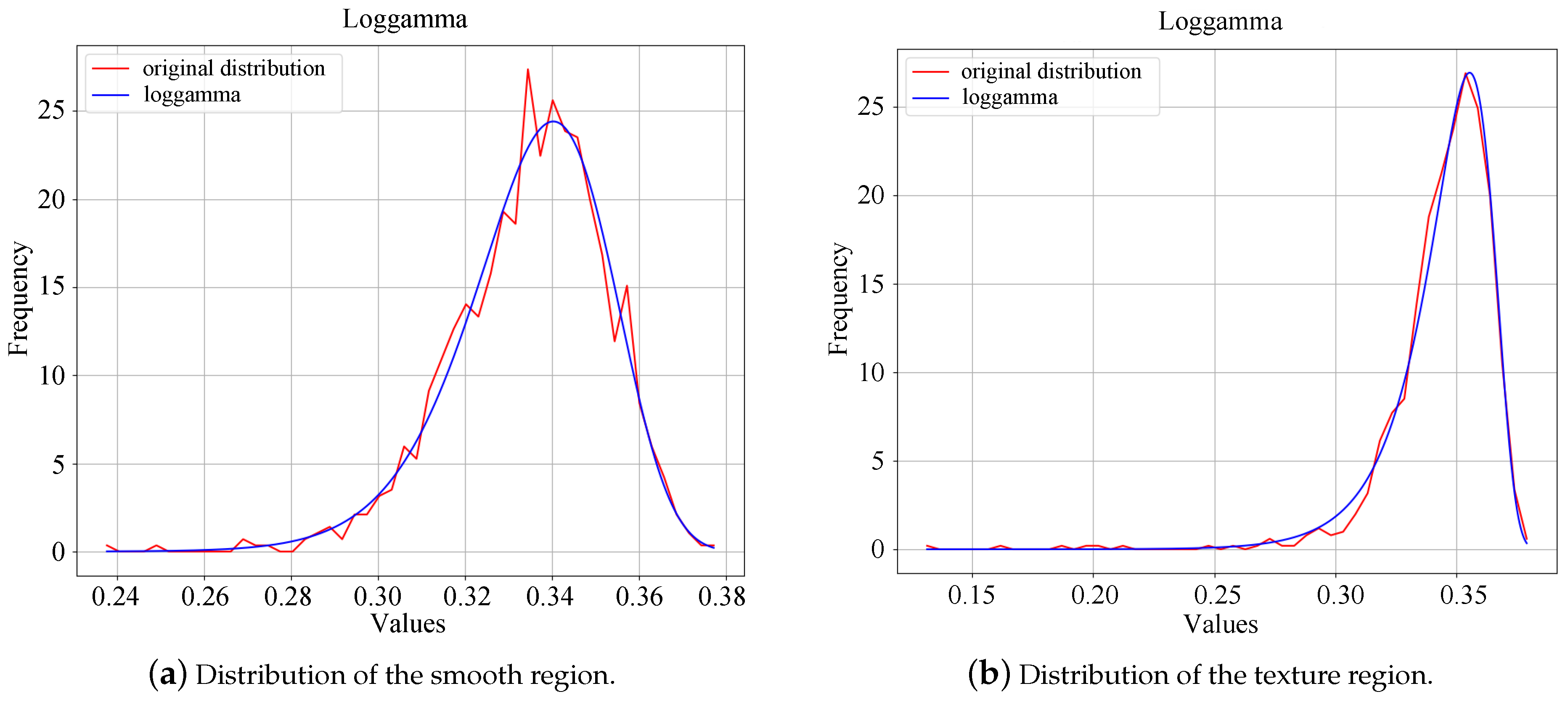
4.3. Characteristic Analysis
4.3.1. Single Sample Characteristics
4.3.2. Cross-Sample Characteristics
4.4. Preprocessing Method


- : repeat step 1;
- : ;
- : .
4.5. Training Algorithm

5. Results
5.1. Experimental Settings
5.1.1. Dataset Introduction
5.1.2. Experimental Environment
5.2. Performance Evaluation
5.2.1. Performance of Different Models
5.2.2. Performance of Each Dataset
5.3. Comparison and Analysis
5.4. Experiments across Datasets
5.4.1. Cross-Coefficient Test
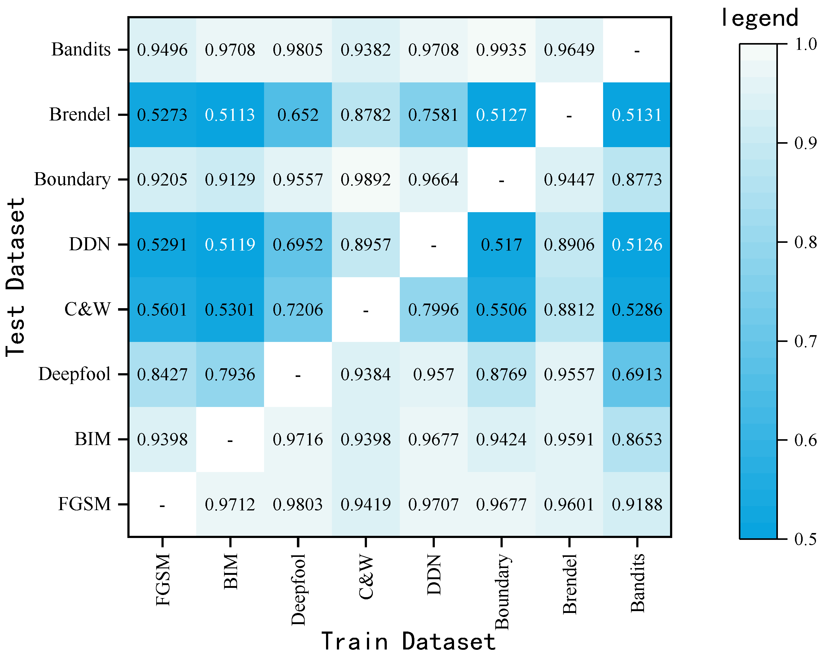
5.4.2. Cross-Attack Method Test
5.5. Multidataset Experiment
5.5.1. Multicoefficient Test
5.5.2. Multimethod Test
6. Conclusions
Author Contributions
Funding
Data Availability Statement
Acknowledgments
Conflicts of Interest
References
- Yang, J.; Zhao, L.; Dang, J.; Wang, Y.; Yue, B.; Gu, Z. A Semantic Segmentation Method for High-resolution Remote Sensing Images Based on Encoder-Decoder. In Proceedings of the 2022 Tenth International Conference on Advanced Cloud and Big Data (CBD), Guilin, China, 4–5 November 2022; pp. 98–103. [Google Scholar] [CrossRef]
- Chen, Z.; Zhao, J.; Deng, H. Global Multi-Attention UResNeXt for Semantic Segmentation of High-Resolution Remote Sensing Images. Remote Sens. 2023, 15. [Google Scholar] [CrossRef]
- Sun, L.; Cheng, S.; Zheng, Y.; Wu, Z.; Zhang, J. SPANet: Successive Pooling Attention Network for Semantic Segmentation of Remote Sensing Images. IEEE J. Sel. Top. Appl. Earth Obs. Remote Sens. 2022, 15, 4045–4057. [Google Scholar] [CrossRef]
- Sun, L.; Ma, C.; Chen, Y.; Zheng, Y.; Shim, H.J.; Wu, Z.; Jeon, B. Low Rank Component Induced Spatial-Spectral Kernel Method for Hyperspectral Image Classification. IEEE Trans. Circuits Syst. Video Technol. 2020, 30, 3829–3842. [Google Scholar] [CrossRef]
- Cheng, G.; Xie, X.; Han, J.; Guo, L.; Xia, G.S. Remote Sensing Image Scene Classification Meets Deep Learning: Challenges, Methods, Benchmarks, and Opportunities. IEEE J. Sel. Top. Appl. Earth Obs. Remote Sens. 2020, 13, 3735–3756. [Google Scholar] [CrossRef]
- Sun, L.; Zhao, G.; Zheng, Y.; Wu, Z. Spectral-Spatial Feature Tokenization Transformer for Hyperspectral Image Classification. IEEE Trans. Geosci. Remote Sens. 2022, 60, 5522214. [Google Scholar] [CrossRef]
- Sun, L.; Fang, Y.; Chen, Y.; Huang, W.; Wu, Z.; Jeon, B. Multi-Structure KELM With Attention Fusion Strategy for Hyperspectral Image Classification. IEEE Trans. Geosci. Remote Sens. 2022, 60, 5539217. [Google Scholar] [CrossRef]
- Kim, M.; Jeong, J.; Kim, S. ECAP-YOLO: Efficient Channel Attention Pyramid YOLO for Small Object Detection in Aerial Image. Remote Sens. 2021, 13, 4851. [Google Scholar] [CrossRef]
- Wu, X.; Li, W.; Hong, D.; Tao, R.; Du, Q. Deep Learning for Unmanned Aerial Vehicle-Based Object Detection and Tracking: A survey. IEEE Geosci. Remote Sens. Mag. 2022, 10, 91–124. [Google Scholar] [CrossRef]
- Goodfellow, I.J.; Shlens, J.; Szegedy, C. Explaining and Harnessing Adversarial Examples. In Proceedings of the 3rd International Conference on Learning Representations (ICLR), San Diego, CA, USA, 7–9 May 2015. [Google Scholar]
- Madry, A.; Makelov, A.; Schmidt, L.; Tsipras, D.; Vladu, A. Towards Deep Learning Models Resistant to Adversarial Attacks. In Proceedings of the 6th International Conference on Learning Representations (ICLR), Vancouver, BC, Canada, 30 April–3 May 2018. [Google Scholar]
- Carlini, N.; Wagner, D.A. Towards Evaluating the Robustness of Neural Networks. In Proceedings of the 2017 IEEE Symposium on Security and Privacy (SSP), San Jose, CA, USA, 22–24 May 2017; pp. 39–57. [Google Scholar] [CrossRef]
- Wang, J.; Zhao, J.; Yin, Q.; Luo, X.; Zheng, Y.; Shi, Y.; Jha, S.K. SmsNet: A New Deep Convolutional Neural Network Model for Adversarial Example Detection. IEEE Trans. Multimed. 2022, 24, 230–244. [Google Scholar] [CrossRef]
- Zhao, J.; Wang, J. Lightweight DCT-Like Domain Forensics Model for Adversarial Example. In Proceedings of the 19th International Workshop on Digital Forensics and Watermarking (IWDW), Melbourne, Australia, 25–27 November 2020. [Google Scholar]
- Grosse, K.; Manoharan, P.; Papernot, N.; Backes, M.; McDaniel, P.D. On the (Statistical) Detection of Adversarial Examples. arXiv 2017, arXiv:1702.06280. [Google Scholar]
- Li, X.; Li, F. Adversarial Examples Detection in Deep Networks with Convolutional Filter Statistics. In Proceedings of the IEEE International Conference on Computer Vision (ICCV), Venice, Italy, 22–29 October 2017; pp. 5775–5783. [Google Scholar] [CrossRef]
- Liu, J.; Zhang, W.; Zhang, Y.; Hou, D.; Liu, Y.; Zha, H.; Yu, N. Detection Based Defense Against Adversarial Examples From the Steganalysis Point of View. In Proceedings of the IEEE Conference on Computer Vision and Pattern Recognition (CVPR), Long Beach, CA, USA, 15–20 June 2019; pp. 4825–4834. [Google Scholar] [CrossRef]
- Moosavi-Dezfooli, S.; Fawzi, A.; Frossard, P. DeepFool: A Simple and Accurate Method to Fool Deep Neural Networks. In Proceedings of the IEEE Conference on Computer Vision and Pattern Recognition (CVPR), Las Vegas, NV, USA, 27–30 June 2016; pp. 2574–2582. [Google Scholar] [CrossRef]
- Rony, J.; Hafemann, L.G.; Oliveira, L.S.; Ayed, I.B.; Sabourin, R.; Granger, E. Decoupling Direction and Norm for Efficient Gradient-Based L2 Adversarial Attacks and Defenses. In Proceedings of the IEEE Conference on Computer Vision and Pattern Recognition (CVPR), Long Beach, CA, USA, 15–20 June 2019; pp. 4322–4330. [Google Scholar] [CrossRef]
- Li, Y.; Wu, B.; Feng, Y.; Fan, Y.; Jiang, Y.; Li, Z.; Xia, S. Semi-supervised robust training with generalized perturbed neighborhood. Pattern Recognit. 2022, 124, 108472. [Google Scholar] [CrossRef]
- Zhang, J.; Xu, X.; Han, B.; Niu, G.; Cui, L.; Sugiyama, M.; Kankanhalli, M.S. Attacks Which Do Not Kill Training Make Adversarial Learning Stronger. In Proceedings of the 37th International Conference on Machine Learning (ICML), Virtual, 13–18 July 2020; Volume 119, pp. 11278–11287. [Google Scholar]
- Song, C.; Fan, Y.; Yang, Y.; Wu, B.; Li, Y.; Li, Z.; He, K. Regional Adversarial Training for Better Robust Generalization. arXiv 2021, arXiv:2109.00678. [Google Scholar]
- Kurakin, A.; Goodfellow, I.J.; Bengio, S. Adversarial examples in the physical world. In Proceedings of the 5th International Conference on Learning Representations (ICLR), Toulon, France, 24–26 April 2017. [Google Scholar]
- Dong, Y.; Liao, F.; Pang, T.; Su, H.; Zhu, J.; Hu, X.; Li, J. Boosting Adversarial Attacks with Momentum. In Proceedings of the IEEE Conference on Computer Vision and Pattern Recognition (CVPR), Salt Lake City, UT, USA, 18–22 June 2018; pp. 9185–9193. [Google Scholar] [CrossRef]
- Ilyas, A.; Engstrom, L.; Madry, A. Prior Convictions: Black-box Adversarial Attacks with Bandits and Priors. In Proceedings of the 7th International Conference on Learning Representations (ICLR), New Orleans, LA, USA, 6–9 May 2019. [Google Scholar]
- Brendel, W.; Rauber, J.; Bethge, M. Decision-Based Adversarial Attacks: Reliable Attacks Against Black-Box Machine Learning Models. In Proceedings of the 6th International Conference on Learning Representations (ICLR), Vancouver, BC, Canada, 30 April–3 May 2018. [Google Scholar]
- Wu, J.; Wang, J.; Zhao, J.; Luo, X.; Ma, B. ESGAN for generating high quality enhanced samples. Multim. Syst. 2022, 28, 1809–1822. [Google Scholar] [CrossRef]
- Xiao, C.; Li, B.; Zhu, J.; He, W.; Liu, M.; Song, D. Generating Adversarial Examples with Adversarial Networks. In Proceedings of the Twenty-Seventh International Joint Conference on Artificial Intelligence (IJCAI), Stockholm, Sweden, 13–19 July 2018; pp. 3905–3911. [Google Scholar] [CrossRef]
- Mangla, P.; Jandial, S.; Varshney, S.; Balasubramanian, V.N. AdvGAN++: Harnessing latent layers for adversary generation. In Proceedings of the IEEE/CVF International Conference on Computer Vision (ICCV), Seoul, Republic of Korea, 27 October–2 November 2019. [Google Scholar]
- Feinman, R.; Curtin, R.R.; Shintre, S.; Gardner, A.B. Detecting Adversarial Samples from Artifacts. arXiv 2017, arXiv:1703.00410. [Google Scholar]
- Schöttle, P.; Schlögl, A.; Pasquini, C.; Böhme, R. Detecting Adversarial Examples—A Lesson from Multimedia Forensics. arXiv 2018, arXiv:1803.03613. [Google Scholar]
- Jia, X.; Wei, X.; Cao, X.; Foroosh, H. ComDefend: An Efficient Image Compression Model to Defend Adversarial Examples. In Proceedings of the IEEE Conference on Computer Vision and Pattern Recognition (CVPR), Long Beach, CA, USA, 15–20 June 2019; pp. 6084–6092. [Google Scholar] [CrossRef]
- Zhao, J.; Wang, J. Recovery of Adversarial Examples based on SmsGAN. J. Zhengzhou Univ. Eng. Sci. 2021, 42, 50–55. [Google Scholar]
- Xu, W.; Evans, D.; Qi, Y. Feature Squeezing: Detecting Adversarial Examples in Deep Neural Networks. In Proceedings of the 25th Annual Network and Distributed System Security Symposium (NDSS), San Diego, CA, USA, 18–21 February 2018. [Google Scholar]
- Kannan, H.; Kurakin, A.; Goodfellow, I.J. Adversarial Logit Pairing. arXiv 2018, arXiv:1803.06373. [Google Scholar]
- Wang, J.; Wang, H.; Li, J.; Luo, X.; Shi, Y.; Jha, S.K. Detecting Double JPEG Compressed Color Images with the Same Quantization Matrix in Spherical Coordinates. IEEE Trans. Circuits Syst. Video Technol. 2020, 30, 2736–2749. [Google Scholar] [CrossRef]
- Wang, H.; Wang, J.; Luo, X.; Zheng, Y.; Ma, B.; Sun, J.; Jha, S.K.J. Detecting Aligned Double JPEG Compressed Color Image with Same Quantization Matrix Based on the Stability of Image. IEEE Trans. Circuits Syst. Video Technol. 2022, 32, 4065–4080. [Google Scholar] [CrossRef]
- Simonyan, K.; Zisserman, A. Very Deep Convolutional Networks for Large-Scale Image Recognition. In Proceedings of the 3rd International Conference on Learning Representations (ICLR), San Diego, CA, USA, 7–9 May 2015. [Google Scholar]
- Brendel, W.; Rauber, J.; Kümmerer, M.; Ustyuzhaninov, I.; Bethge, M. Accurate, reliable and fast robustness evaluation. In Proceedings of the Annual Conference on Neural Information Processing Systems 2019 (NIPS), Vancouver, BC, Canada, 8–14 December 2019; pp. 12841–12851. [Google Scholar]
- He, K.; Zhang, X.; Ren, S.; Sun, J. Deep Residual Learning for Image Recognition. In Proceedings of the IEEE Conference on Computer Vision and Pattern Recognition (CVPR), Las Vegas, NV, USA, 27–30 June 2016; pp. 770–778. [Google Scholar] [CrossRef]
- Zagoruyko, S.; Komodakis, N. Wide Residual Networks. In Proceedings of the Proceedings of the British Machine Vision Conference 2016 (BMVC), York, UK, 19–22 September 2016. [Google Scholar]
- Huang, G.; Liu, Z.; van der Maaten, L.; Weinberger, K.Q. Densely Connected Convolutional Networks. In Proceedings of the IEEE Conference on Computer Vision and Pattern Recognition (CVPR), Honolulu, HI, USA, 21–26 July 2017; pp. 2261–2269. [Google Scholar] [CrossRef]
- Gao, S.; Cheng, M.; Zhao, K.; Zhang, X.; Yang, M.; Torr, P.H.S. Res2Net: A New Multi-Scale Backbone Architecture. IEEE Trans. Pattern Anal. Mach. Intell. 2021, 43, 652–662. [Google Scholar] [CrossRef]


| adversarial example(s) | |
| clean example corresponding to adversarial example | |
| clean example | |
| label(s) of | |
| x[i] | the ith element in matrix x |
| JPEGquality factor used when testing | |
| number of training epochs with | |
| multiplication of corresponding elements in matrices | |
| back propagation | |
| combine the input data | |
| statistical cleaning | |
| cross entropy of and | |
| generate random numbers that follow the x distribution | |
| JPEG compression and decompression with quality factor f | |
| number of elements in matrix x | |
| select a batch of data from x | |
| classification model with input x | |
| all-1 matrix with the same size as x | |
| randomly select an element from x | |
| natural number sequence from 0 to x | |
| all-0 matrix with the same size as x |
| ResNet18 | ResNet34 | ResNet50 | ResNet101 | Res2Net50 | ||
| = 2 | 99.07% | 98.65% | 97.86% | 97.99% | 97.89% | |
| 100.39% | 99.87% | 99.85% | 100.21% | 99.65% | ||
| = 4 | 99.54% | 99.35% | 99.52% | 99.04% | 99.03% | |
| 99.83% | 99.63% | 99.88% | 102.61% | 101.23% | ||
| = 6 | 99.92% | 99.83% | 99.89% | 99.64% | 99.70% | |
| 100.03% | 100.01% | 100.05% | 99.81% | 100.41% | ||
| = 8 | 99.91% | 99.94% | 99.87% | 99.89% | 99.94% | |
| 99.98% | 100.02% | 99.98% | 99.96% | 100.02% | ||
| WideResNet50 | WideResNet101 | DenseNet169 | VGG11 | VGG16 | ||
| = 2 | 97.38% | 98.11% | 96.92% | 97.05% | 97.72% | |
| 98.47% | 99.03% | 99.28% | 98.22% | 99.45% | ||
| = 4 | 99.70% | 99.42% | 99.02% | 98.37% | 99.50% | |
| 99.83% | 99.56% | 99.61% | 98.75% | 100.13% | ||
| = 6 | 99.92% | 99.85% | 99.80% | 99.13% | 99.65% | |
| 100.20% | 99.96% | 99.98% | 99.31% | 99.80% | ||
| = 8 | 99.91% | 99.98% | 99.83% | 99.88% | 99.87% | |
| 100.02% | 100.01% | 99.90% | 100.23% | 100.03% | ||
| ResNet18 | ResNet34 | ResNet50 | ResNet101 | Res2Net50 | ||
| = 2 | 96.25% | 96.69% | 95.78% | 96.13% | 95.84% | |
| 98.96% | 99.21% | 98.55% | 98.65% | 98.67% | ||
| = 4 | 98.41% | 98.01% | 98.62% | 98.27% | 97.84% | |
| 99.35% | 99.15% | 99.91% | 99.48% | 99.30% | ||
| = 6 | 99.28% | 98.96% | 99.08% | 98.81% | 99.06% | |
| 99.85% | 99.59% | 99.99% | 99.63% | 99.74% | ||
| = 8 | 99.54% | 99.59% | 99.47% | 99.25% | 99.23% | |
| 99.86% | 99.93% | 99.84% | 99.75% | 99.69% | ||
| WideResNet50 | WideResNet101 | DenseNet169 | VGG11 | VGG16 | ||
| = 2 | 96.47% | 96.09% | 92.16% | 95.96% | 92.40% | |
| 98.90% | 98.51% | 100.45% | 98.66% | 121.77% | ||
| = 4 | 98.33% | 97.71% | 97.80% | 97.78% | 98.33% | |
| 99.30% | 98.74% | 99.83% | 98.68% | 114.54% | ||
| = 6 | 99.21% | 99.45% | 99.46% | 99.30% | 99.07% | |
| 99.54% | 99.73% | 100.65% | 99.84% | 101.29% | ||
| = 8 | 99.37% | 99.49% | 98.57% | 98.98% | 99.27% | |
| 99.59% | 99.83% | 99.18% | 99.31% | 101.12% | ||
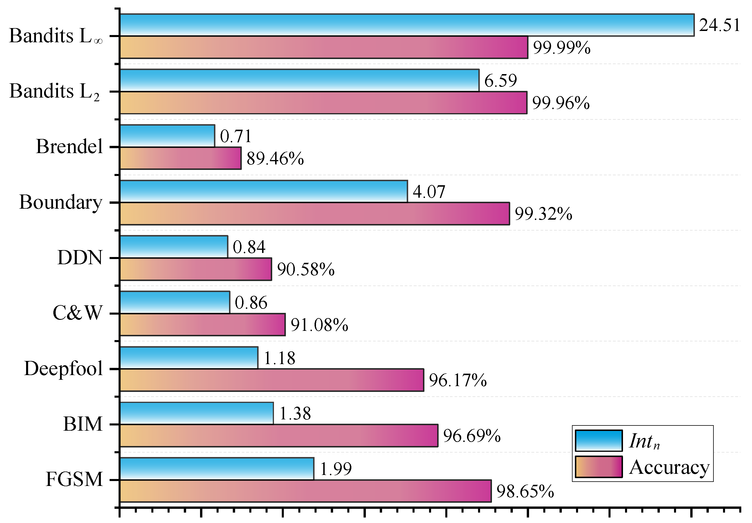
| FGSM | 1.99 | 3.97 | 5.93 | 7.91 |
| BIM | 1.38 | 2.29 | 3.15 | 3.68 |
| Ours | ESRM [17] | SmsNet [13] | DCT-Like [14] | |
|---|---|---|---|---|
| FGSM | 98.65% | 98.10% | 98.49% | 99.64% |
| BIM | 96.69% | 97.14% | 99.27% | 99.18% |
| Deepfool | 96.17% | 95.13% | 98.26% | 99.07% |
| C&W | 91.08% | 92.87% | 93.83% | 95.02% |
| Test | = 2 | = 4 | = 6 | = 8 | |
|---|---|---|---|---|---|
| Train | |||||
| FGSM | |||||
| = 2 | accuracy | - | 99.07% | 98.78% | 98.92% |
| recall | - | 99.91% | 99.82% | 99.86% | |
| = 8 | accuracy | 51.14% | 86.87% | 99.57% | - |
| recall | 3.23% | 74.22% | 99.84% | - | |
| BIM | |||||
| = 2 | accuracy | - | 97.16% | 97.27% | 97.37% |
| recall | - | 99.96% | 99.98% | 99.97% | |
| = 8 | accuracy | 85.89% | 92.61% | 98.99% | - |
| recall | 83.32% | 86.59% | 99.65% | - | |
| = 2 | = 4 | = 6 | = 8 | Overall | |
|---|---|---|---|---|---|
| FGSM | 98.63% | 99.32% | 99.31% | 98.53% | 99.20% |
| BIM | 96.15% | 98.97% | 99.36% | 99.21% | 98.42% |
| FGSM | BIM | Deepfool | C&W | |
| Accuracy | 97.20% | 96.98% | 96.24% | 97.36% |
| DDN | Boundary | Brendel | Bandits | |
| Accuracy | 87.82% | 96.81% | 84.08% | 97.12% |
Disclaimer/Publisher’s Note: The statements, opinions and data contained in all publications are solely those of the individual author(s) and contributor(s) and not of MDPI and/or the editor(s). MDPI and/or the editor(s) disclaim responsibility for any injury to people or property resulting from any ideas, methods, instructions or products referred to in the content. |
© 2023 by the authors. Licensee MDPI, Basel, Switzerland. This article is an open access article distributed under the terms and conditions of the Creative Commons Attribution (CC BY) license (https://creativecommons.org/licenses/by/4.0/).
Share and Cite
Zhao, J.; Wu, J.; Adeke, J.M.; Qiao, S.; Wang, J. Detecting High-Resolution Adversarial Images with Few-Shot Deep Learning. Remote Sens. 2023, 15, 2379. https://doi.org/10.3390/rs15092379
Zhao J, Wu J, Adeke JM, Qiao S, Wang J. Detecting High-Resolution Adversarial Images with Few-Shot Deep Learning. Remote Sensing. 2023; 15(9):2379. https://doi.org/10.3390/rs15092379
Chicago/Turabian StyleZhao, Junjie, Junfeng Wu, James Msughter Adeke, Sen Qiao, and Jinwei Wang. 2023. "Detecting High-Resolution Adversarial Images with Few-Shot Deep Learning" Remote Sensing 15, no. 9: 2379. https://doi.org/10.3390/rs15092379