Improving Semantic Segmentation of Roof Segments Using Large-Scale Datasets Derived from 3D City Models and High-Resolution Aerial Imagery

Abstract

Advances in deep learning techniques for remote sensing as well as the increased availability of high-resolution data enable the extraction of more detailed information from aerial images. One promising task is the semantic segmentation of roof segments and their orientation. However, the lack of annotated data is a major barrier for deploying respective models on a large scale. Previous research demonstrated the viability of the deep learning approach for the task, but currently, published datasets are small-scale, manually labeled, and rare. Therefore, this paper extends the state of the art by presenting a novel method for the automated generation of large-scale datasets based on semantic 3D city models. Furthermore, we train a model on a dataset 50 times larger than existing datasets and achieve superior performance while applying it to a wider variety of buildings. We evaluate the approach by comparing networks trained on four dataset configurations, including an existing dataset and our novel large-scale dataset. The results show that the network performance measured as intersection over union can be increased from 0.60 for the existing dataset to 0.70 when the large-scale model is applied on the same region. The large-scale model performs superiorly even when applied to more diverse test samples, achieving 0.635. The novel approach contributes to solving the dataset bottleneck and consequently to improving semantic segmentation of roof segments. The resulting remotely sensed information is crucial for applications such as solar potential analysis or urban planning.

1. Introduction

In recent years, much attention has been devoted to and significant advances have been made in the application of deep learning (DL) techniques to the semantic segmentation of remote sensing imagery in general and the extraction of building footprints in particular [1,2,3]. The obtained spatial information enables manifold applications in environmental and urban analysis and planning, but their manual acquisition is time-consuming and therefore costly. Challenges that are encountered in this area of research include the variety and semantics of visible objects, the spatiotemporal variability in their appearance, occlusions by other image contents, resulting difficulties in accurately separating objects and identifying their boundaries, highly imbalanced class distributions, and the availability of annotated training data [3,4,5].

The extraction of building footprints is a task that is addressed frequently, and various innovative methods have been explored that tackle the described problems. While the application of DL for the semantic segmentation of building footprints in remote sensing images promises a cost-effective automation of a previously laborious manual process, effective training of DL models requires large amounts of annotated data, which by itself is costly and time-consuming to procure if labeling is performed manually. Solution approaches to reduce labeling costs focus either on improving training efficiency with the limited data available (model-centric) or on finding ways to cost-efficiently generate larger annotated datasets (data-centric), and in some cases a combination of both is investigated. In the former category, Kang et al. [6] and Hua et al. [7] propose semi-supervised learning methods where only a limited amount of the training data is labeled. In the latter category, several studies investigate the use of publicly available data (e.g., OpenStreetMap) to automatically generate large-scale datasets for training and evaluation of neural networks [5,8,9,10,11,12,13]. Nevertheless, a prevalent weakness of these approaches is a certain misalignment between the derived labels and the remote sensing images.

As semantic segmentation of building footprints matures, researchers turn to the task of extracting even more detailed building information from aerial images. Some authors use classic computer vision approaches to identify individual roof segments and their orientation in aerial images [14,15]. To the best of our knowledge, three more recent publications apply semantic segmentation by means of DL for this task [16,17,18]. A popular application of this information is solar potential analysis, but mapped roof segments and their orientation can be useful for other fields such as urban planning as well. However, a major barrier for DL approaches remains the availability of datasets.

Lee et al. [16] introduced and first applied the manually labeled DeepRoof dataset. They distinguish sixteen azimuth classes for sloped segments in 22.5${}^{\circ }$ bins and one class for flat segments. Krapf et al. [17] also used the DeepRoof dataset and additionally explored the semantic segmentation of roof superstructures. In a subsequent work, Krapf et al. [19] published RID (the roof information dataset), which includes labels for roof segments as well as roof superstructures. Li et al. [18] used RID, designed a multi-task network architecture, and reduced the number of classes for sloped roof segments to four, based on the insight that sixteen classes disproportionately deteriorate model performance while four classes reduce this problem and are still sufficient for accurate solar potential estimation.

To the best of our knowledge, the only datasets for semantic segmentation of roof segments are the DeepRoof dataset [16] and the RID [19]. They feature 2274 and 1880 buildings with 4312 and >4500 manually labeled roof segments, respectively. In both cases, the labeled aerial images are sourced from small geographic regions and the diversity of roof geometries, building contexts, lighting conditions, and image quality is limited. The applicability of models trained on these rather homogeneous datasets to regions with different properties is therefore limited [19]. A larger and more heterogeneous dataset comprising labeled imagery from diverse regions and settings could improve model performance and applicability, but, as in the case of building footprints and semantic segmentation datasets in general, such data is costly and time-consuming to produce manually [20].

Accordingly and similar to the problem of building footprint extraction and training of artificial neural networks in general, the shortage of annotated training data hampers a further improvement of the models’ performance. Contrary to the case of building footprints, on the other hand, publicly available map data cannot be used to automatically generate large-scale training datasets because they do not contain information about roof segments. However, semantic 3D city models according to the CityGML standard [21,22] are today available for many towns and cities worldwide. In many cases, they are published by public authorities and are openly accessible free of charge [23]. They represent detailed building data with roof and wall surfaces described both semantically and geometrically, which could be used to derive roof segment labels for aerial images and, thus, to cost-efficiently generate more heterogeneous large-scale datasets featuring a wider variety of roof geometries and other properties. Based on this insight, this paper presents a novel approach for cost-effectively generating a versatile large-scale dataset for semantic segmentation of roof segments from aerial images using 3D city models, representing a wide range of geometrical and geographical conditions. To evaluate the dataset, this paper investigates the effectiveness of the automatically created large-scale dataset in comparison to the existing, manually labeled RID by training convolutional neural networks (CNNs) on both datasets.

The aims of the present study can be summarized into the following research questions, which are answered and discussed throughout this article:

1.

How can semantic 3D city models be used to generate heterogeneous large-scale datasets of roof segment labels for aerial images?

2.

Which label characteristics and potential inaccuracies must be expected when using such an approach?

3.

How does the segmentation performance of a convolutional neural network model differ when trained on small-scale, homogeneous, manually labeled data compared to large-scale, heterogeneous, automatically labeled data?

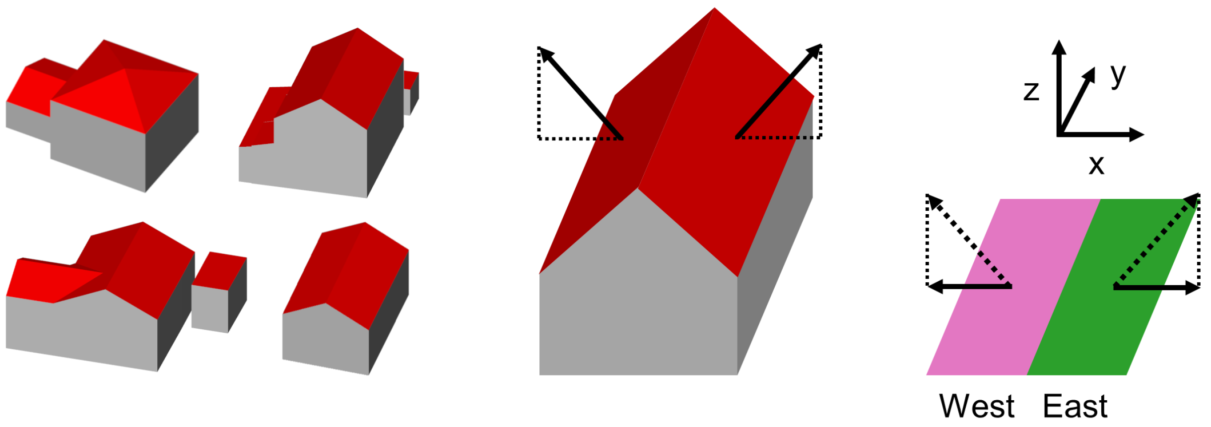
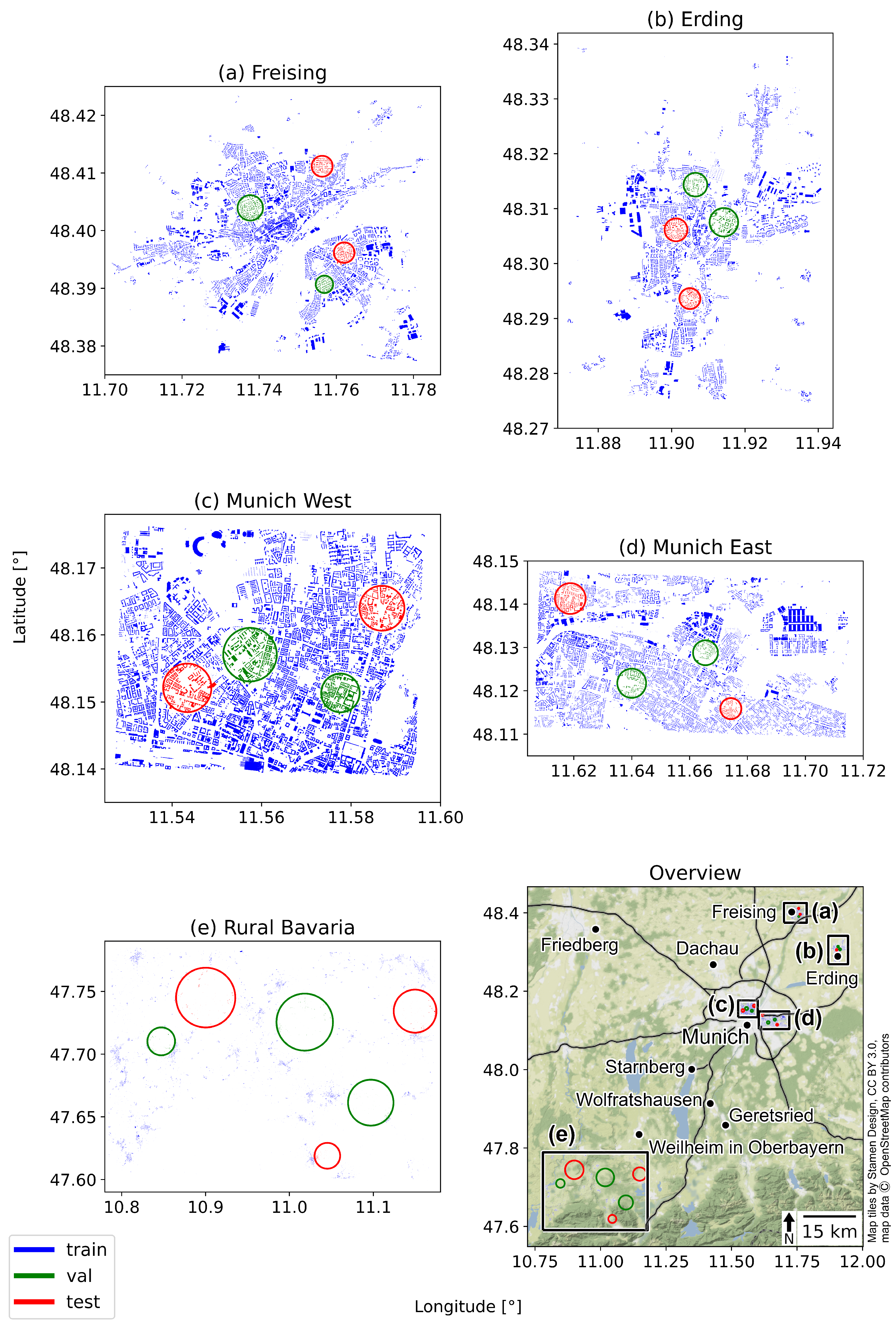
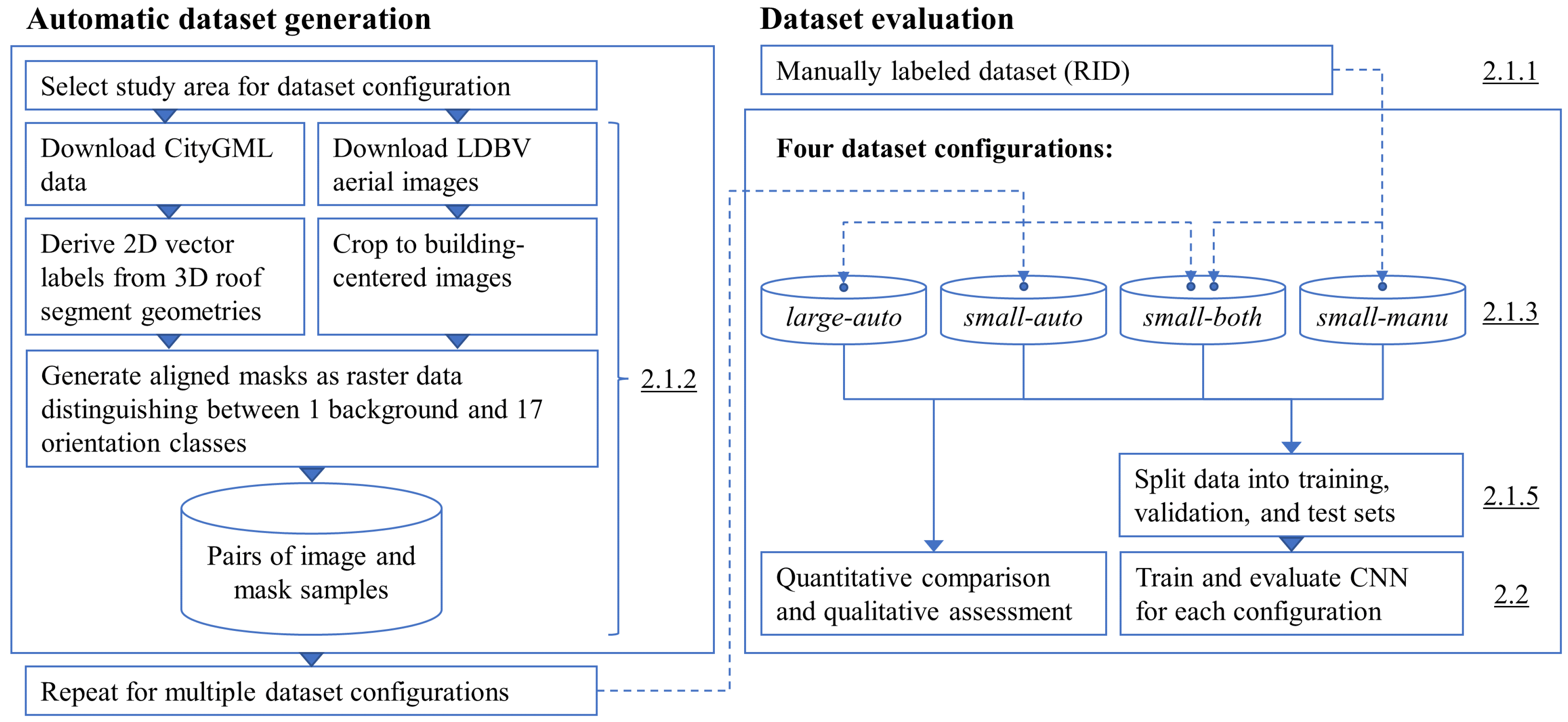
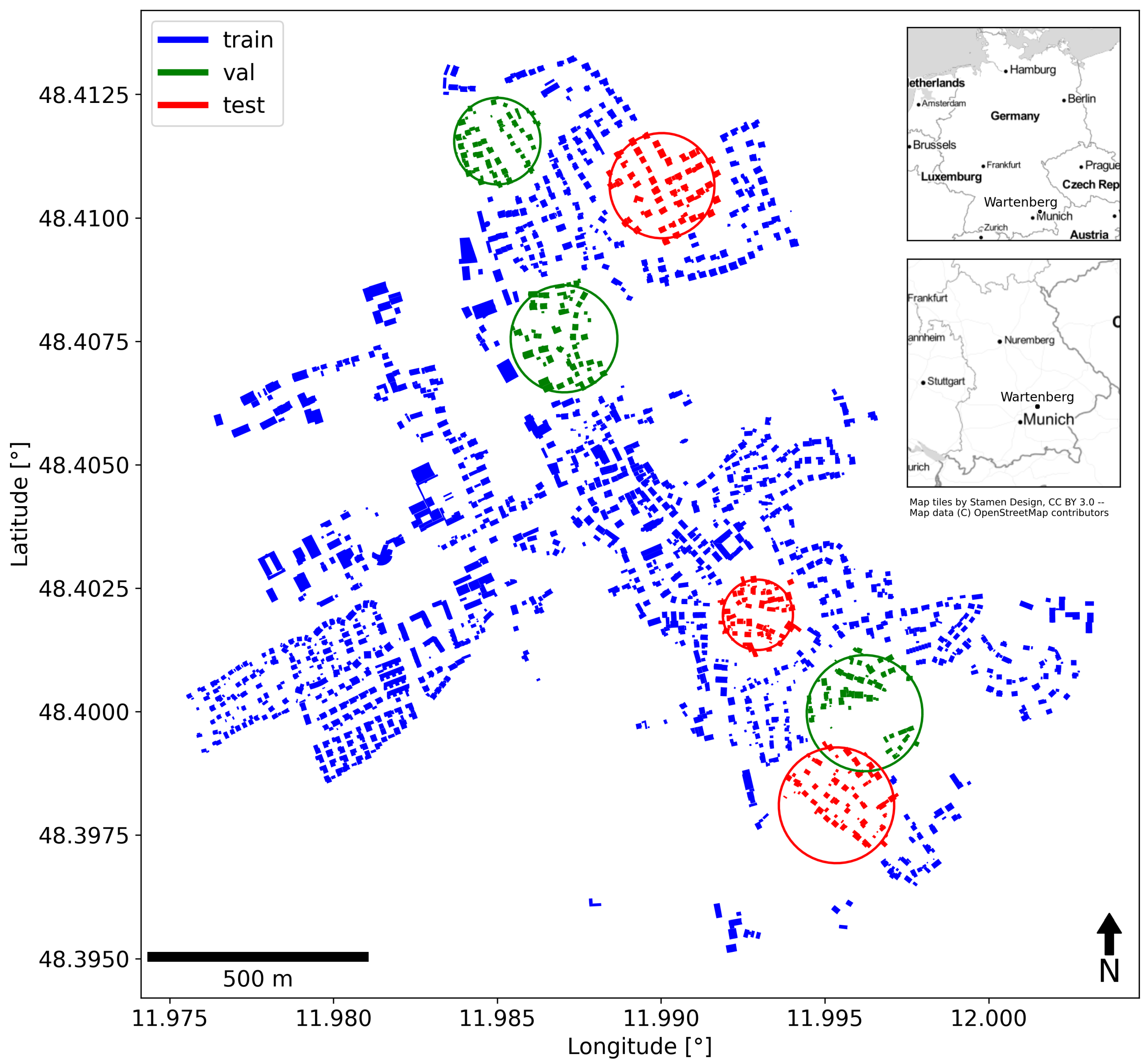
To this end, a set of study areas in southern Germany was selected that reflects diverse settlement conditions. Using a 3D city model, we created a large-scale training dataset in the form of digital orthophotos and roof segments masks reflecting 18 classes, similarly to DeepRoof [16] and RID [19]. Additionally, the manually labeled RID [19] was recreated in an automated fashion using this study’s novel approach. Both the original and the recreated RID served as comparison to evaluate our large-scale dataset and the model that was trained on it. The datasets were split into subsets for training, validation, and testing with the aim to reduce the introduction of a spatial bias. With regard to research question 1, the approach to dataset generation and all configurations are described in Section 2.1. A convolutional neural network adopting the U-Net architecture [24] was trained on each of the datasets. Details about the hyperparameters, training procedure, and evaluation metrics are provided in Section 2.2. The results comprise a detailed comparison between the manually and automatically generated datasets with respect to research question 2 (Section 3.1). Furthermore, and in response to research question 3, an evaluation of the networks’ semantic segmentation performance (Section 3.2) and exemplary model predictions are examined (Section 3.3). The discussion (Section 4) provides further answers to questions 2 and 3 by reviewing implications and limitations of the findings and giving suggestions for improvements as well as a comparison to the state of the art.

The contributions of this article include:

• A novel approach for generating labeled datasets from 3D city models and aerial images for semantic segmentation of roof segments,
• The exemplary generation of such a large-scale dataset that is more than 50 times as large as the state of the art,
• A model that predicts roof segments and their orientation with a mean IoU of 0.70, which surpasses the state of the art, is capable of generalizing to a significantly larger variety of roofs, and distinguishes more orientation classes,
• A discussion of opportunities and challenges in using 3D city models for automatically generating such datasets.

2. Materials and Methods

Figure 1 gives an overview of the methodology and indicates in which sections the respective steps are described in detail. The following Section 2.1 explains the approach to automatically generate large-scale datasets of roof segment labels from aerial images using 3D city models and thereby provides an answer to research question 1. Subsequently, Section 2.2 covers the neural network architecture, hyperparameters, and metrics used for training and evaluation.

2.1. Datasets and Configurations

2.1.1. Manually Labeled Baseline Dataset

The RID (Roof Information Dataset for Computer Vision-Based Photovoltaic Potential Assessment [19]) was used as a baseline configuration. It features manually annotated, georeferenced polygon geometries for all roof segments of 1880 buildings in the German village of Wartenberg based on Google aerial imagery at 0.1 m px${}^{-1}$ resolution. Additionally, for each building it provides a building-centered $512\times 512$ px aerial image crop and a corresponding mask with labels.

The masks were generated by rasterization and pixel-wise classification of the segments’ geometries. Three sets of masks are available where, depending on their azimuth, sloped roof segments are assigned to one of 4, 8, or 16 classes. In all cases, flat roof segments are represented by a separate class, and all other areas are labeled as background. For the present study, the set of masks with the finest subdivision of sloped roofs into 16 azimuth classes was used, which accordingly distinguishes between a total of 18 different semantic classes (see

Table 1. Pixel-level classification of samples: background, 16 orientation classes for sloped roof segments with the corresponding azimuth ranges, flat roof class.

ID	Class Name	Abbr.	Azimuth Range [°]
			Min	Max
0	Background	BG	-	-
1	North	N	−11.25	11.25
2	North-northeast	NNE	11.25	33.75
3	Northeast	NE	33.75	56.25
4	East-northeast	ENE	56.25	78.75
5	East	E	78.75	101.25
6	East-southeast	ESE	101.25	123.75
7	Southeast	SE	123.75	146.25
8	South-southeast	SSE	146.25	168.75
9	South	S	168.75	191.25
10	South-southwest	SSW	191.25	213.75
11	Southwest	SW	213.75	236.25
12	West-southwest	WSW	236.25	258.75
13	West	W	258.75	281.25
14	West-northwest	WNW	281.25	303.75
15	Northwest	NW	303.75	326.25
16	North-northwest	NNW	326.25	348.75
17	Flat	Flat	-	-

).

To ensure conformity with the aerial imagery used for the automatically labeled samples as described in the following, each RID sample was resized to $256\times 256$ px.

2.1.2. Automated Annotation of Aerial Images Using 3D City Models

CityGML is a data modeling standard for semantic 3D cities and landscape models. It represents spatial objects on five different levels of detail and comprises information on their geometry, semantics, topology, and appearance [21,22]. The geometry of city objects is described by boundary representation (B-rep), where solids are defined by an aggregation of their bounding surfaces. Hence, all roof segments are modeled separately as constituting boundary surfaces of the respective buildings.

For the selected study areas (see Section 2.1.3), 3D city data according to the CityGML specification were available at level of detail 2 (LOD2), which includes roof structures. Each planar roof segment is represented by a single, equally planar polygon. Therefore, projection of the roof segment polygons onto the two-dimensional, horizontal plane enables the generation of labels for digital orthophotos. Their orientation in space allows deduction of their azimuth and slope for classification of the labels. This is performed by computing each segment’s normal vector and translating its horizontal (x and y) components into an angle relative to the north direction: the azimuth. Subsequently, an orientation class is assigned to the roof segments which corresponds to a discretization of the continuous azimuth. Figure 2 illustrates this approach.

Both the CityGML data and the corresponding true orthophotos at 0.2 m px${}^{-1}$ resolution were obtained from the Bavarian Agency for Digitisation, High-Speed Internet and Surveying LDBV (Landesamt für Digitalisierung, Breitband und Vermessung) [25]. The geometric accuracy of the 3D building models in the source CityGML data is determined by their generation method: Building footprints are sourced from the official German cadastral land register ALKIS (Amtliches Liegenschaftskatasterinformationssystem); their absolute accuracy is better than 5 cm. The 3D building model is then automatically generated using airborne laser-scanning 3D point cloud data and the commercial software BuildingReconstruction (its method is explained in [26]), available from virtualcitysystems GmbH, and roof geometry is generalized according to CityGML LOD2 (no dormers, no chimneys).

For processing, the CityGML data were imported to a PostgreSQL database with PostGIS extension and a 3DCityDB [27,28] instance for processing. 3DCityDB is an open source implementation of CityGML as data model for spatial relational databases. The roof segments were queried and exported with their required attributes:

• The segment’s identifier (ID),
• The ID of the associated building,
• The projected, two-dimensional segment polygon geometry,
• The segment’s azimuth and slope as computed from its normal vector using a custom function in Procedural Language/PostgreSQL (PL/pgSQL),
• The roof generation method (see Section 2.1.4).

All further processing was performed in Python. The samples were generated as pairs of $256\times 256$ px LDBV aerial image crops and masks containing the labels, centered on the building centroids. At this size, most buildings were contained completely within the image and only few very large buildings extended beyond the image boundaries. Depending on their azimuth and slope, roof segments were assigned to one of 17 classes: sloped roofs were categorized into 16 orientation classes, subdividing the 360${}^{\circ }$ range into 22.5${}^{\circ }$ slices, and flat roofs into a separate class. All other areas were labeled as background, amounting to a total of 18 different semantic classes (see Table 1), which corresponds to the labeling logic used in the RID dataset. The code used to generate the datasets is available at [29].

2.1.3. Dataset Configurations and Study Areas

Table 2. Dataset configurations and data splits: numbers of samples in total and in training, validation, and test sets, and number of geographical positions from which validation and test samples were selected.

	Number of Samples				Number of Positions
Configuration	Total	Training	Validation	Test	Validation	Test
small-manu	1878	1364	180	180	3	3
small-auto	1878	1364	180	180	3	3
small-both	3756	2728	360	360	3	3
large-auto	94,490	84,312	4500	4500	11	11

presents the dataset and training configurations with sample numbers and details about the data split, which is discussed further in Section 2.1.5. Figure 3 and Figure 4 provide a visualization of the data and study areas. The manually labeled RID dataset, as introduced in Section 2.1.1, served as a baseline configuration (small-manu). For a second configuration, the RID dataset was recreated based on 3D city data and LDBV aerial images to obtain a structurally identical, but automatically labeled dataset with equal number (1878) and spatial distribution of building samples (small-auto). This enables evaluating the influence of the different aerial imagery sources used in the manual and automatic labeling approaches on training outcome.

The potential of the approach to derive roof segment labels for aerial images from semantic 3D city data lies in the possibility to automatically generate large and diverse datasets. To leverage this potential, a large-scale dataset (large-auto) was created from a variety of regions in southern Bavaria, which were selected with the aim to maximize the diversity of building types present in the data. For this purpose, the Regional Statistical Spatial Typology for Mobility and Transport Research (RegioStaR) by the German Federal Ministry for Digital and Transport BMDV (Bundesministerium für Digitales und Verkehr) was used, and in particular, the combined regional statistical spatial type RegioStaR 17 [30]. Areas with a total of 123,050 buildings were selected that are distributed as follows: 58,580 buildings from central Munich (types 111 metropolis and 112 large city from regional type 11 metropolitan urban region), 30,808 buildings from the regional towns of Erding and Freising (type 113 medium-sized city from regional type 11 metropolitan urban region), and 33,662 buildings from a large rural area southwest of Munich (types 225 small-town area, village area and 224 urban area from regional type 22 peripheral rural region).

For a fourth configuration, the RID dataset and the identically structured, automatically generated dataset were combined (small-both). Aerial images from Google and LDBV differ in terms of time of day (shadows), camera angle, contrast, etc. This adds to the difference between manual and automatic annotation and results in different samples for the same building. The aim of this configuration is to examine to what extent a neural network trained only on one of these two types of datasets specializes on them or is capable of generalizing to the other type of dataset, compared to a network that was trained using data from both approaches.

2.1.4. Pre-Processing of the Large-Scale Dataset

In the case of the large-scale dataset large-auto, an additional preparatory step was required due to the properties of the underlying 3D city data. Each roof’s geometry is generated by an algorithm that attempts to identify it from an airborne laser-scanning 3D point cloud which, upon failure, assigns a default flat roof at a height derived from other parameters. This leads to a corresponding number of buildings for which the roof representation in the data likely does not match their real geometry and, therefore, incorrect roof segment labels would be created from the 3D city data. A generic attribute indicates the roof generation method of each CityGML building and allows identification of buildings to which a default flat roof geometry was assigned [31].

As shown in

Table 3. Distribution of the large-scale dataset by roof generation method of the 3D city data: numbers of buildings and single roof segments for each method. Classification according to [31].

Roof Generation Method		Object Count
Value	Description	Buildings	Segments
1000	Identification algorithm (automatic)	61,581	98,776
2000	Identification algorithm (semi-automatic, edited)	54,560	196,308
3100	Unidentified: Flat roof with minimum height	1398	1398
3210	Unidentified: Flat roof with derived height (automatic)	3425	3425
3220	Unidentified: Flat roof with derived height (edited)	1855	1855
4000	Manual input of roof geometry	0	0
9999	Unknown	231	542
	Sum	123,050	302,304

, for a total of 6678 (5.4%) of the 123,050 buildings the roof geometry could not be identified reliably and a flat roof was assigned consequently (values 3100, 3210, 3220). To ensure validity of all automatically generated labels appearing in samples, all samples intersecting any of these buildings had to be discarded. Of the original number of 123,050 samples in the large-scale dataset, 94,490 samples remained following this pre-processing step. All roof geometries were identified correctly in the case of the small-scale dataset small-auto.

2.1.5. Dataset Split Considering Spatial Overlap

For each configuration, all data were subdivided into datasets for training, validation, and testing of the respective neural network model. Due to the samples being centered on building centroids and their spatial distribution, in some cases buildings appear fully or partially in more than one sample. Therefore, if a sample is assigned to one of the subsets, it must be ensured that no sample intersecting it is assigned to any of the other subsets to warrant that the sets are disjointed.This can be achieved by defining the three subsets consecutively and, in an intermediate step after the definition of each set, discarding all samples intersecting the ones assigned to the respective set. Several approaches to sample selection for subset definition are conceivable. A completely random selection would be ideal to achieve three identically distributed subsets without spatial bias. However, a comparatively large number of samples would have to be discarded in this case to ensure that the sets are disjoint.

Therefore, in order to maximize the number of samples that can be used for training, validation, and testing while minimizing spatial bias, a spatially based data split was performed as follows. Within the data region, several positions were chosen for both the test and validation set along with a specific number of buildings to be selected around each of these positions. First, around each test position, this pre-defined number of buildings was identified within a circular area whose radius was determined iteratively. These buildings were then subtracted from the main dataset. To ensure that the datasets are entirely disjoint, i.e., that no parts of buildings contained fully or partially in the test set are depicted in any of the other sets, all buildings intersecting the extent of the samples selected for the test set were also subtracted from the source dataset. Based on the remaining buildings, the identical procedure was then repeated for the chosen validation positions to find the buildings for the validation set. Following that, all remaining buildings comprised the training set. Because of the approach that was used to ensure that the datasets are disjointed as described here, the sum of the numbers of training, validation, and test set samples is smaller than the total number of samples for a given configuration.

Table 2 shows numbers of subset samples for each of the configurations. For the RID dataset small-manu and the identically structured, automatically generated dataset small-auto, three positions were selected for both the validation and test set. Sizes of validation and test set were selected to account for approximately 10% of the total number of samples, resulting in a split ratio of approximately 80:10:10. For the composite dataset small-both, the sets were combined. As described in Section 2.1.3, the large-scale dataset large-auto consists of data from several regions in Bavaria. A total of 11 positions for both the validation and test set were selected and distributed across these regions: four in the rural area southwest of Munich, three in the central Munich area, and two each in the smaller cities of Erding and Freising. For each region, the numbers of validation and test set samples were chosen to account for approximately 5% of the respective region’s total number of samples, resulting in a split ratio of approximately 90:5:5.

Table 4. Distribution of validation and test set samples across the regions in the large-scale dataset.

Large-Scale	Number of Samples
Dataset Region	Total (Relative)		Test	Validation	Per Position	Positions Per Set
Rural Bavaria	25,128	(0.27)	1200	1200	400	3
Munich	41,945	(0.44)	2000	2000	500	4
Erding, Freising	27,417	(0.29)	1300	1300	325	4
All	94,490	(1.00)	4500	4500

gives an overview of this. Figure 3 and Figure 4 show a geographical representation of the datasets and their corresponding training, validation, and test set areas.

2.2. Dataset Evaluation and Semantic Segmentation Training

The quality of the datasets generated as described in the previous sections is evaluated in three ways: first, by means of a quantitative comparison in terms of mean IoU to the manually labeled dataset (which is possible for the configurations small-auto and small-manu), as well as a qualitative comparison between the two. Second, by a thorough qualitative assessment of label characteristics and potential random and systematic inaccuracies. Third, the datasets are evaluated with respect to their intended application: The training of neural networks for the task of semantic segmentation of roof segments in aerial imagery. An analysis of the resulting models’ performance enables the identification of strengths and weaknesses compared to the manually labeled dataset, the influence of dataset and label characteristics, and, hence, an informed discussion of the datasets’ applicability for the designated task.

2.2.1. Neural Network Architecture and Hyperparameters

For each comparison configuration, a convolutional neural network (CNN) was trained for 40 epochs. Similar to Krapf et al. [17], we selected the U-Net architecture [24] with a ResNet-152 backbone [32] in an implementation following [33]. This study takes a data-centric approach, where the main focus is investigating the influence of different datasets on the training outcome, and therefore neglects the implementation of a specialized network architecture. Several loss functions designed to handle highly imbalanced class distributions (e.g., in the automatically labeled small-scale dataset, 79% of all pixels belong to the background class) were explored [34,35], and the categorical focal loss was found to deliver the best results. Due to hardware limitations and network depth, the batch size could only be set as high as 8 samples. Adam was used as an optimizer [36] and learning rate was set to ${10}^{-4}$ and decreased by a factor of 10 whenever a plateau was reached during training.

2.2.2. Data Augmentation

To decrease overfitting and improve the network’s ability to generalize, the training data was augmented in the following ways during training while preserving the validity of the orientation labels: resizing and shifting, addition of Gaussian noise, change of brightness, contrast, saturation, and gamma value, sharpening, and blurring.

2.2.3. Neural Network Performance Evaluation

Intersection over union (IoU) was used as a metric for the evaluation of model performance. It is is defined as

$$IoU=\frac{TP}{TP+FP+FN},$$

(1)

where $TP$, $FP$, and $FN$ refer to the numbers of true positives, false positives, and false negatives, respectively. On the image level, IoU is first computed for each class, then the average of all class IoU values is taken. Similarly, on the dataset level, IoU is computed for each class across the dataset and the average of all class IoU values is taken. This corresponds to a macro average (as opposed to a weighted macro or micro average [37]) and ensures that each class is weighted equally in the final IoU value, which delivers more informative results considering the imbalanced class distribution in the datasets used here. In either case, IoU values for classes that are absent in the image and whose absence is predicted correctly (i.e., union is zero) are excluded from the average, as opposed to setting IoU to one for these classes and including it. With regard to the large number of classes, this approach enables a more meaningful representation of segmentation performance on classes that are actually present. It does, however, in many cases result in lower scores.

3. Results

The first section of the results chapter aims to answer research question 2 by identifying characteristics and potential inaccuracies of the generated roof segment labels. Following it, the results in terms of semantic segmentation performance are presented and illustrated with exemplary model predictions, which provide a comprehensive answer to research question 3.

3.1. Automatically Generated Labels and Their Quality

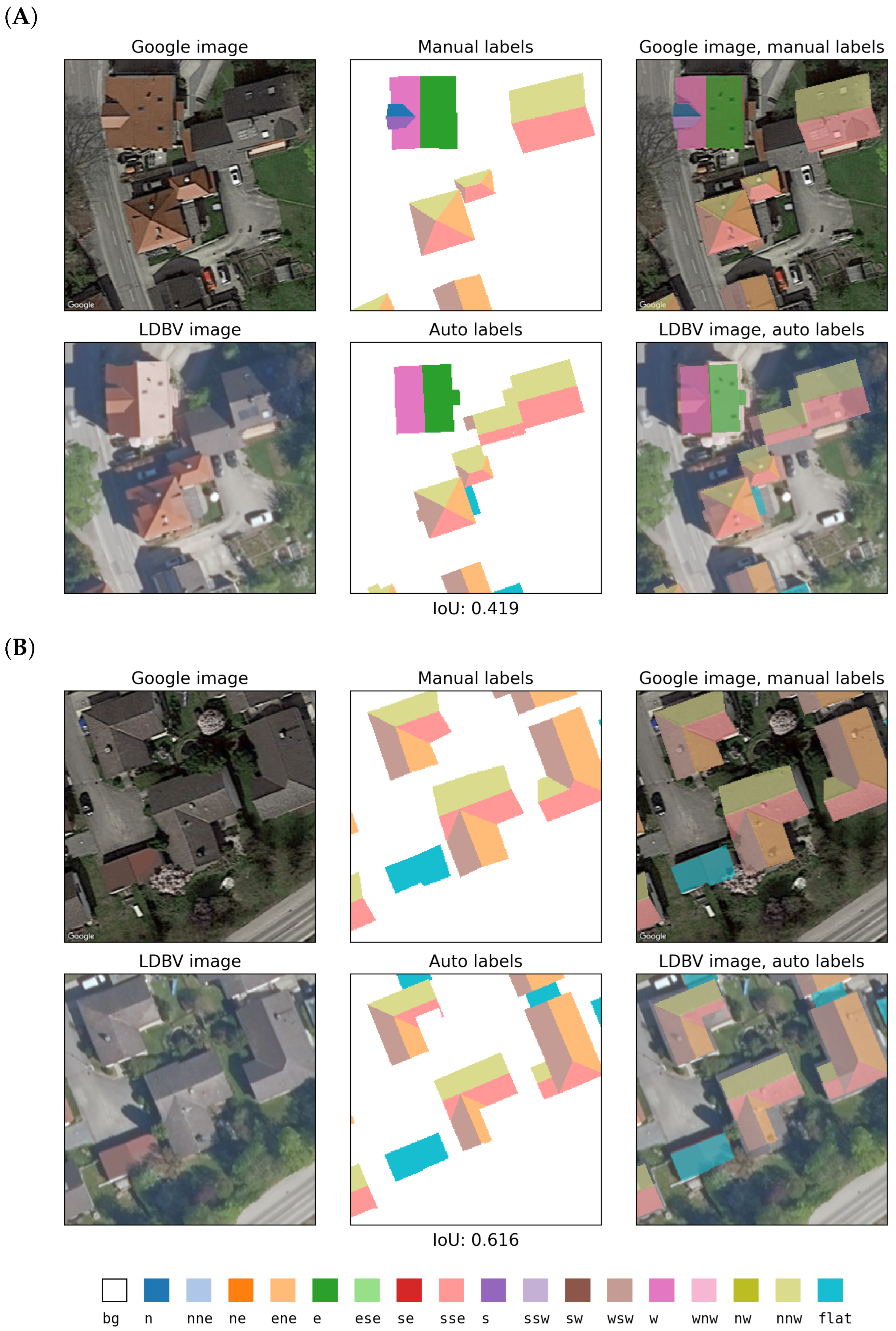
Because the samples of the two corresponding configurations small-manu and small-auto cover the same area around identical locations (the building centroids), it is possible to compare them with respect to their quality and consistency. Figure 5 gives an exemplary graphical comparison showing two training samples from both datasets. Overall, the automatically generated labels are well aligned to the roofs as depicted in the aerial imagery, and their representation of the roof geometries is largely very accurate. This points to their suitability for the training of neural networks.

The manually labeled RID dataset is based on Google aerial imagery, while the automatically labeled datasets use LDBV true orthophotos to warrant congruence with the 3D city data. Hence, a certain degree of misalignment between the two is to be expected. To obtain a quantitative measure, their IoU was computed and found to be 0.49. While this indicates some degree of consistency, several sources for discrepancies between the two datasets and, thus, their labels can be identified. They are described in the following and can be observed in the samples shown in Figure 5, which were selected to illustrate them.

For both datasets there are cases where one provides more detailed labels than the other; for instance, with respect to the individual delineation of dormers or their omission. Qualitative assessment of random samples indicates that, generally, dormers are more often delineated individually in the manual dataset. Furthermore, roof geometries in the LOD2 3D city model in some cases are simplified to an extent that leads to an incorrect representation of some roof parts in the derived labels, particularly for cross-gabled buildings with one or several wings. The manual dataset in general only has labels for visible roofs, while the automatically generated labels also cover roof areas that may be hidden underneath vegetation in the LDBV images.

Because the LOD2 3D city data used here do not model roof overhangs whereas they are of course visible in the aerial imagery, the automatic labels in many cases do not cover the depicted roofs completely, i.e., to their edges. The effect of this systematic inaccuracy on the performance of the models could, for instance, be investigated by labeling a certain amount of LDBV image samples manually including roof overhangs, training a model on these data, and comparing its results to those of a model trained on 3D-city-data-derived labels.

Finally, there are cases in which the assignment of an orientation class differs between the manual and automatic datasets. This occurs when a roof segment’s orientation is at the boundary between two classes. Then, the outcome of the manual labeling process may fall in one orientation class while the orientation computed from the segment’s normal vector in the 3D city data results in the other orientation class. Potential effects on segmentation performance are unclear and could be investigated separately in the future, but are considered likely to be negligible because of the small number of cases and the fact that, at the boundary between two classes, the orientation of a segment is not always unambiguous between the datasets due to small differences in angles. Therefore, the assignment of either class cannot with certainty be considered wrong taking into account the context of the underlying data. Similarly, either model output could be considered correct within the margins of uncertainty.

3.2. Semantic Segmentation Performance

3.2.1. Mean Intersection over Union

Table 5. Intersection over union of all four models evaluated on each of the four test datasets (names in italics), computed as described in Section 2.2.3.

	Dataset
Model	small-manu	small-auto	small-both	large-auto
small-manu	0.603	0.425	0.513	0.366
small-auto	0.369	0.584	0.470	0.411
small-both	0.602	0.616	0.609	0.467
large-auto	0.504	0.700	0.597	0.635

lists the performance of all four models in terms of intersection over union as described in Section 2.2.3, evaluated on each of the four configurations’ test sets. One finds a clear separation between the model trained on manually labeled samples and those trained on automatically labeled samples, but also between the small-scale models and the model trained on the large-scale dataset. The same holds true for the corresponding test datasets and the models’ results on these.

With an IoU of 0.603 and 0.602, respectively, the models small-manu and small-both are the best performers on the manually labeled dataset small-manu. The first was trained on this particular dataset and, therefore, can be expected to be specialized on it. The latter, which was trained on the combined small-scale datasets (both manually and automatically labeled), achieves practically equal, but not superior performance. Additional exposure to automatically labeled LDBV images during training seems not to have translated into an improvement in its ability to segment Google imagery, but also not to have impeded it. The large-scale model large-auto with an IoU of 0.504 scores higher than the model small-auto (0.369) only trained on the automatically labeled small-scale dataset, indicating an improvement from training on an extended LDBV image dataset when required to generalize to Google data with manual labels.

With respect to the dataset small-auto, the large-scale model large-auto scores highest at 0.700, again providing evidence for the benefit arising from dataset extension. The models small-both and small-auto, which were trained on automatically labeled data as well, achieve IoU values of 0.616 and 0.584, respectively. The first performs slightly better, which might be attributed to its exposure to additional, albeit manually labeled Google imagery during training. The worst performing model on the automatically labeled small-scale dataset unsurprisingly is the one that was not exposed to any corresponding training data, but only to manually labeled data: small-manu with an IoU of 0.425.

On the dataset small-both combining both the manually and automatically labeled small-scale datasets, the corresponding model that was trained on this exact dataset scores highest at 0.609. It is closely followed by the model large-auto with an IoU of 0.597. While this may at first glance appear to indicate that training on an extended, automatically labeled dataset also enhances segmentation performance on manually labeled data, the large-auto model’s results on the datasets small-manu and small-auto tell otherwise, where it performs rather poorly on the first and very good on the second. This illustrates the fact that evaluation on a combined dataset can be misleading, since the same mean IoU value may be achieved by different distributions of performance across the included image sources.

The evaluation results on the large-auto test dataset show the lowest IoU scores on average. This could be expected considering that it is the most challenging dataset with very heterogeneous data from rural and urban areas across Bavaria, where especially the urban parts differ significantly from the rural small-town area represented in the small-scale datasets. The model large-auto trained on the corresponding training data achieves the highest score at 0.635. Among the remaining three models, the one that was exposed to both manually and automatically labeled data in training (small-both) performs best at 0.467, again indicating a carryover effect from increased training data heterogeneity even if the source of the additional data is different. It is followed by the model small-auto, achieving an IoU of 0.411. Finally, the model small-manu, which was trained only on the small and manually labeled dataset, shows the poorest performance with an IoU of 0.366.

With respect to the main diagonal in Table 5, which represents the evaluation of the four models on their own test datasets, it is noteworthy that the model large-auto performs best, considering that it was both trained and tested on the most diverse, heterogeneous, and, therefore, challenging configuration.

Regarding the small-scale models and in view of the performance on the manually labeled test dataset small-manu, it appears that combining manually and automatically labeled training data does not translate into a performance improvement compared to training only with manually labeled data. Conversely, if evaluated on an automatically labeled dataset (small-auto or large-auto), a model that during training was exposed to both manually and automatically labeled data outperforms one that was trained exclusively on automatically labeled data. Overall, one can observe a significant degree of specialization among the models on the data used for training and only limited ability to generalize to data of different composition and quality, but also a clear improvement in model versatility from combining heterogeneous data during training.

3.2.2. Confusion Matrices

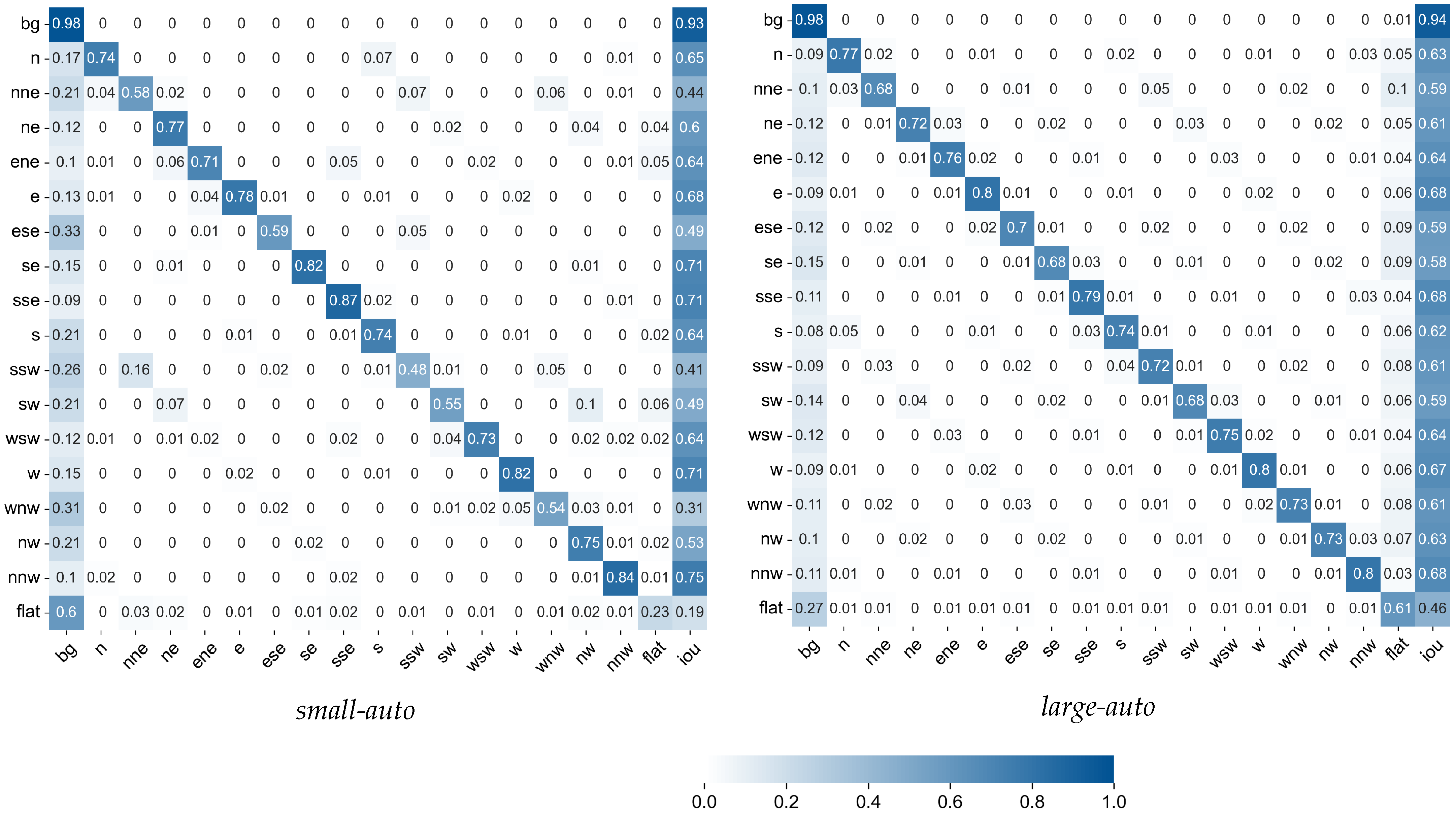
Figure 6 compares confusion matrices of the models small-auto and large-auto evaluated on their own test sets. Several notable observations can be made: in both cases, the background class is the one that is identified most reliably, followed by the sloped roof segment classes. Flat roofs pose a challenge to both models, and the model small-auto classifies the majority as background, which is reflected in a low class IoU of 0.19. The model large-auto also has difficulties identifying flat roofs but performs significantly better.

While the background class is identified very well, it is also the one that is most frequently assigned falsely to pixels that belong to roof segments. This points to the problem arising from the highly imbalanced class distribution. Although a loss function suitable for such data was used in training, it nevertheless could not completely prevent the development of a model bias to predict the background class with higher frequency. Another observable pattern is that sloped roof segments are with some, however lesser, frequency classified as flat.

Both models have a slight tendency to confuse sloped roof segment classes with orthogonal azimuths. For example, while most north-facing roof segments are identified correctly, a certain number is also classified as facing east, south, or west. This is understandable considering that such roof segments would mainly differ by lighting, whereas any textures such as roof tile patterns would have a similar orientation.

Across all these characteristics, the model small-auto shows a higher variability than the model large-auto, which is mainly due to the small dataset in which not all classes are represented equally. Variability aside, the model large-auto performs better overall, confirming the finding in terms of mean IoU described in Section 3.2.1.

3.3. Model Prediction Examples

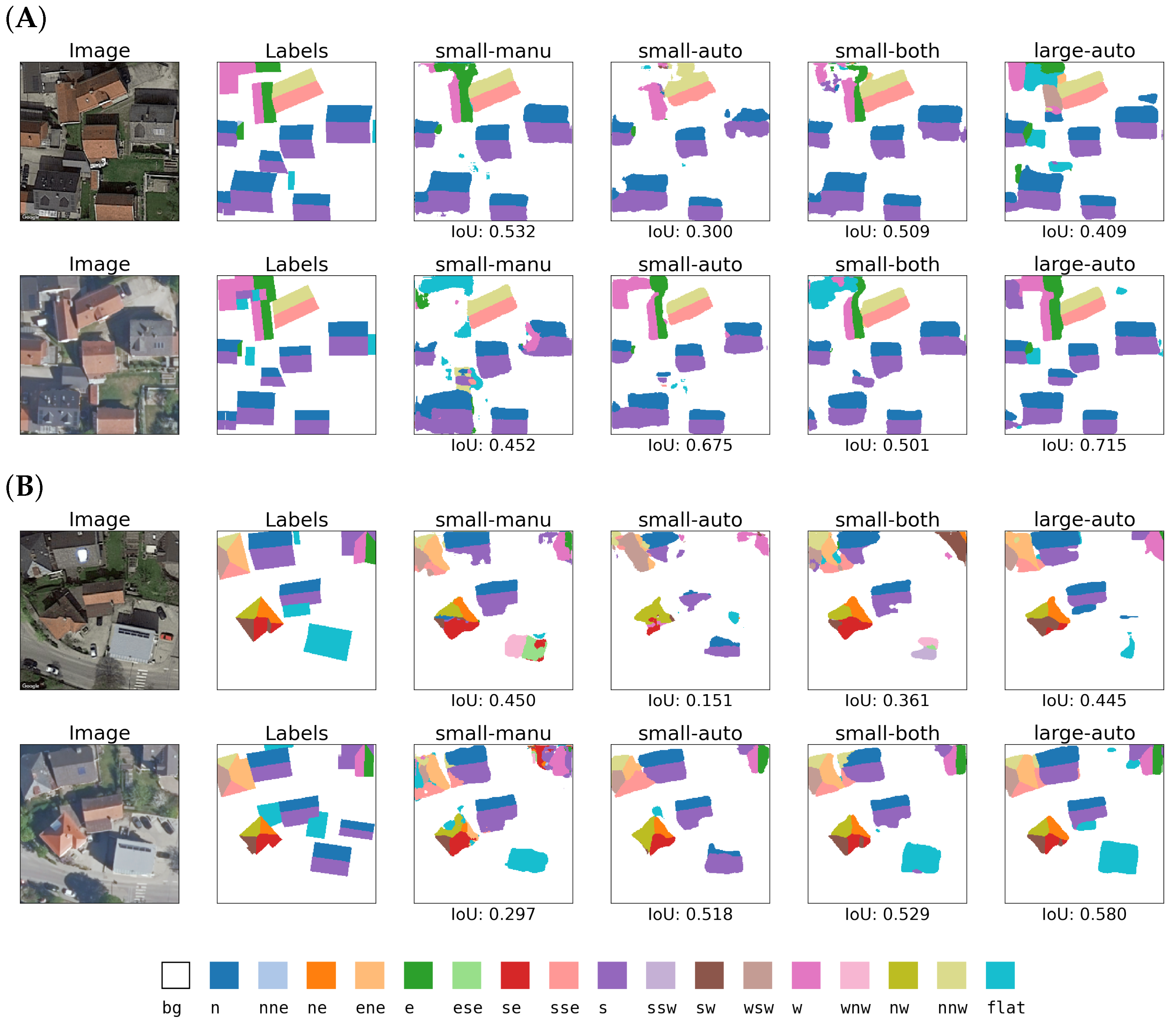
Figure 7 shows predictions of all four models when evaluated on samples from the manually and automatically labeled small-scale datasets at identical locations. They illustrate similarities and differences in model behavior and between the data sources. It is immediately apparent that the image quality differs, with the Google image crops being slightly sharper and higher in contrast compared to the LDBV imagery. A possible reason could be a post-processing of the Google images that enhances these attributes.

The samples from location (A) contain residential buildings with roofs predominantly sloped towards north and south. Manual and 3D-city-data-derived labels show good consistency overall, with the manual labels omitting a few small roof areas in the north-western part of the sample. The models small-manu and small-both perform best on the Google image (upper row), the first scoring slightly higher in terms of IoU. Both models trained solely on automatically labeled data score lower. The large-auto model’s prediction delivers better roof outlines, but a higher IoU score is hindered mainly by predictions of flat roofs that are not present in the labels and failure to accurately detect the roof structures at the north-western position.

Roof segments in the corresponding LDBV image (lower row) at the same location are predicted best by the large-scale model large-auto. It is the only one capable of correctly identifying and outlining several of the smaller roof structures in the picture. The models small-auto and small-both follow in this order sorted by performance, correlated inversely to the number of samples they were trained on. The model small-manu, trained exclusively on manually labeled Google images, clearly has difficulties interpreting the LDBV image, delivering largely inaccurate segment predictions, which is reflected in its IoU being the lowest among all examples from this location.

Location (B) contains two pyramid roofs, which generally pose a greater challenge to the networks due to their lower frequency in the training data. Comparison of the labels at the location reveals a roof that was falsely classified as flat in the manual data. The available two-dimensional information did not allow the labeling person to identify its gable geometry. The automatically generated labels, on the other hand, contain an additional gable roof where in the LDBV image only a parking lot is visible, possibly due to outdated data. Regarding predictions on the Google image (upper row), none of the models manages to deliver convincing results, in particular with respect to the pyramid roofs. Quantitatively, the models small-manu and large-auto score highest, but their predictions do not seem sufficient for practical application.

In view of the predictions on the LDBV image sample (lower row) at location (B), one can observe that three of the models underlie the same misinterpretation as the human labeler, classifying the roof in the south-eastern corner of the sample as flat. The pyramid roofs are outlined well by the models large-auto and small-both, while the other two have difficulties. The model small-manu, not exposed to automatically labeled LDBV images in training, manages to identify some segments but fails with many, which is reflected in the lowest IoU score. The discrepancy between the ground truth labels and the objects actually visible in the LDBV image crop leads to overall lower IoU values in this example.

These examples confirm the observation made in the overall results that there is significant specialization on the data source the models were trained on, and this is comprehensible considering the systematic differences in image and label quality. The results of the models small-both and large-auto illustrate that both a more diverse training dataset composed from both sources and an extended, purely automatically labeled dataset can lead to an improvement in segmentation performance on either data source.

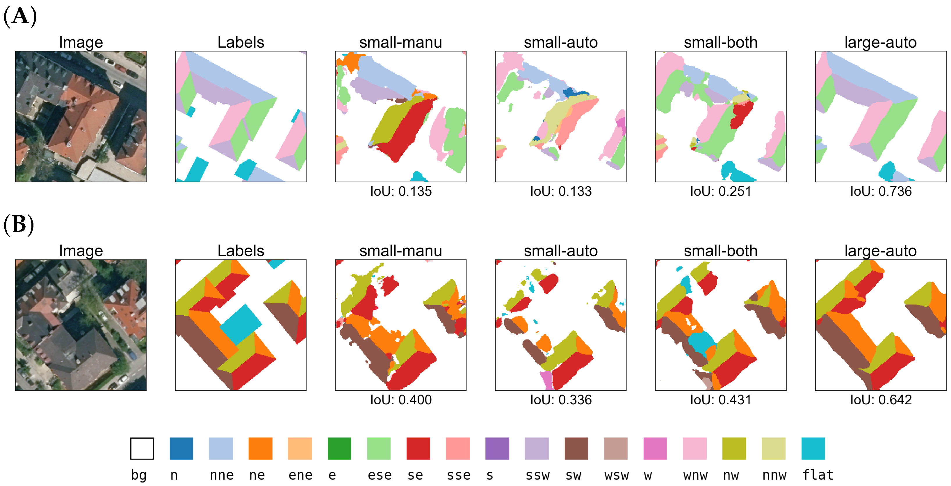
Figure 8 provides predictions from all four models on two samples from the large-scale dataset large-auto showing buildings from an urban residential environment in Munich, reflected in larger and more coherent roof structures. Since manually labeled samples are not available at these locations, a comparison between automatically and manually labeled samples as provided for the small-scale datasets is not possible here.

At both locations (A) and (B), the model large-auto scores highest by a significant margin, which meets the expectations considering that only this model was trained on data from similar environments. Qualitatively, it is capable of delivering very accurate outlines of the individual roof segments and of identifying their orientations correctly. The flat roofs that are present in the labels at the south-western corner of location (A) and centrally at location (B) are not predicted because they are hardly visible or covered by vegetation in the corresponding images, which also limits the maximum achievable IoU on these samples. The three models that were trained on the small-scale datasets largely fail to produce usable results. In many cases, they manage to identify correct orientations but fail to detect complete segments. Notably, the model small-both scores highest among the three in both examples, again indicating an improvement in capability to generalize from training on mixed data.

4. Discussion

The first part of this chapter provides further insights with respect to research question 2 by discussing properties of the automatically generated datasets. The second part reviews the observed semantic segmentation performance in a wider context and is therefore relevant to research question 3.

4.1. Generation of Datasets from Semantic 3D City Model Data

4.1.1. Characteristics of the Derived Labels

As described in Section 3.1, qualitative and quantitative assessment of the 3D-city-data-derived roof segment labels shows good consistency with the corresponding aerial images as well as compared to the manually labeled dataset. This validates the applicability of semantic 3D city models for the task and allows for an effective training of neural networks, as is substantiated by the results presented here.

Nevertheless, roof segment labels that were derived from semantic 3D city data can exhibit certain characteristics that reflect properties of the data source and may be disadvantageous. In the case of the data used here, a drawback is their oftentimes incomplete coverage of visible roof areas due to roof overhangs not being represented in the 3D city model. While the discrepancy is small in most cases, it can become a problem from two perspectives. First, IoU as a performance measure loses meaning: a perfect IoU of predictions with respect to the labels would not imply perfect model performance in the desired manner, but rather that many roof segments are predicted incompletely. Conversely, a perfect model performance in extracting roof segments would not be reflected in a perfect IoU. Second, one could argue that, in these cases, the 3D-city-data-derived labels do not teach the model to identify roof segments but to predict the extent of the underlying building footprint. The manifestation of this is visible in some of the example prediction masks provided in Section 3.3, where the model small-manu predicts slightly larger roof segments than the models small-auto and large-auto. Semantic 3D city models that include roof overhangs could solve this problem. The availability of such datasets is more limited, but may improve in the future. For instance, the Swiss dataset swissBUILDINGS3D 2.0 already provides nation-wide coverage of building models with roof overhangs for Switzerland [38]. In addition, if manual labels were available for a part of the automatically labeled imagery, this would allow performance quantification with respect to the actual prediction target, i.e., complete roof segments.

To further improve the quality of the automatically generated labels, a threshold value could be implemented for the distinction between flat and sloped roofs. So far, any roof with non-zero slope as computed from its normal vector was classified as sloped. Among all 123,050 (302,304) buildings (segments) in the original large-scale CityGML data, 59,532 segments from 45,333 buildings are not sloped (including the 6678 buildings for which a default flat roof was assigned because their roof geometry could not be identified), 4199 segments from 2733 buildings have a slope smaller 5${}^{\circ }$, and 17,637 segments from 11,118 buildings have a slope smaller than 10${}^{\circ }$. It is conceivable that many of these barely sloped roofs are hard to distinguish from flat roofs in the images. This would suggest a potential further improvement in training effectiveness and model performance if they were classified as flat in the label generation process.

4.1.2. Implications of the Approach to Splitting the Datasets

Moreover, there is room for improvement concerning the approach to splitting the datasets into subsets for training, validation, and testing. Under ideal conditions, all datasets would follow the same distribution, but this is difficult to achieve with spatially heterogeneous data. The approach used in this study was selected for several reasons.

Firstly, it aims at reducing spatial bias by allowing the selection of several locations for each of the subsets around which their samples are selected, instead of only one location. While this helps reduce the bias somewhat, it certainly does not eliminate it entirely. It would be better to select the subset samples completely at random. This would, however, lead to a greater reduction of usable samples than the lumped approach taken here, because all samples intersecting buildings (or rather, segments) that themselves intersect validation or test set samples cannot be used in any of the other sets. Another promising approach could be to generate grid-based instead of roof-centered samples. By means of shifting the grid by a fraction of the cell size one could further increase the number of samples, equaling a pre-training augmentation strategy.

Secondly, the used approach was thought to best reflect the real-world application of the neural network model in identification of a building’s roof segments, where they would appear in the image center. Further, it would ensure that most buildings could be depicted fully within the spatial extent of their training sample, whereas in a grid-based dataset, the likelihood of buildings being cut off at the image edges is, on average, higher.

4.1.3. Scalability of the Data Generation Approach

Finally, the dataset of LDBV images with labeled roof segments that was generated and investigated here is, with 94,490 samples, considerably larger than the manually labeled datasets DeepRoof by Lee et al. [16] and RID by Krapf et al. [19]. Nevertheless, the wide availability of aerial imagery and semantic 3D city data in many countries would enable the generation of datasets that could be larger by an order of magnitude and further increase the diversity of represented contexts. This could help to establish whether the discussed shortcomings of the 3D-city-data-based labels is a limiting factor or if segmentation performance could be improved further.

Moreover, it would allow us to investigate to which degree the model that was trained here is capable of generalizing to data from other cities and regions. This is a question that, as of now, cannot be answered due to the lack of datasets with semantically labeled roof segments (other than DeepRoof and RID), which is a gap that this study aims to fill. Subsequent work could shed light on this matter by preparing and generating such datasets using the approach introduced here.

4.2. Semantic Segmentation Performance

4.2.1. Overall Performance Evaluation and Its Limitations

Overall, the models trained on the automatically labeled datasets deliver good results. The model small-auto performs comparably to the model small-manu when evaluated on their own test datasets, and the model large-auto performs superior both on the small-scale test dataset and its own, large-scale test dataset, which features a significantly increased variety of roof geometries. However, the specialization of the models on the corresponding type of training data (Google and LDBV aerial imagery, respectively) impedes ideal comparability between them. In order to unambiguously identify any improvements achieved by using a large-scale, 3D-city-data-based dataset with its potential drawbacks instead of a smaller but manually labeled dataset, it would be better if the latter were based on the same image material, i.e., LDBV imagery. This would enable identification of the impact of label characteristics that are introduced by properties of the 3D city data as described above, and to separate this from the additional effect of network specialization on data source.

Furthermore, any interpretation of the results depends on the measure used for their quantification and comparison. There are several ways to compute the seemingly unambiguous intersection over union metric, and they emphasize different qualities in the predictions [37]. The results must therefore be interpreted with respect to the method of computation. Depending on the scenario at hand, one metric’s advantage can become a drawback, and vice versa. For instance, a micro-averaged IoU has the advantage that a weighting of classes by their frequency is implied, which helps avoid the influence of very small classes that are predicted badly if the larger classes show good results. On the other hand, if there is one class (like the background class) that is exceedingly more frequent than all other classes, a model that mostly predicts this class obtains a result that is good in terms of this measure but not meaningful. For this reason, a macro-averaged mean IoU was used here that weights the results of all classes equally.

The importance of an appropriate application and interpretation of object detection and segmentation performance metrics in consideration of their inherent limitations is also being discussed in recent literature [39,40]. Further, IoU as a performance measure cannot be optimized directly in training because it is non-differentiable in some cases. Several new, IoU-derived loss functions that aim to circumvent this problem were proposed in recent work, both for object detection [41] and semantic segmentation, such as an adaptation by van Beers et al. [42] or a generalized IoU for pixelwise prediction (PixIoU) by Yu et al. [43].

4.2.2. Possibilities to Improve Segmentation Performance

Considering the finding that the neural networks show a significant specialization on the data source they were trained on and that data augmentation alone does not suffice to overcome this limitation, one could try to find approaches that allow better generalization to other sources of remote sensing imagery. This was already investigated in a first attempt by combining the datasets small-manu and small-auto into a single dataset small-both and, indeed, it helped the corresponding neural network to achieve good performance on data from both Google and LDBV aerial images. A next step could be to apply the same approach to the large-scale model.

Similar methods were successfully employed in the case of building footprint extraction from aerial imagery: Maggiori et al. [9] trained a fully convolutional network (FCN) first on a high volume of less accurate data generated using OpenStreetMap (OSM) and, in a second step, on a small set of manually labeled data. This fine-tuning step improved the IoU score achieved by their FCN from 0.48 to 0.66. Kaiser et al. [8] report promising results after conducting a variety of experiments using manually annotated data and Google images with OSM labels. They trained FCNs either exclusively on automatically or hand-labeled data, or pre-train on the former and fine-tune on the latter.

A problem that can be observed in the exemplary prediction masks presented in Section 3.3 are inaccurate roof segment boundaries. Frequently, the presence, approximate location, and orientation of roof segments are predicted correctly, but the models have difficulties identifying accurate outlines and predict rather irregular shapes. This hampers practical applicability and is reflected in lower performance metrics.

The same problem is encountered in the related task of building footprint extraction, has been investigated in numerous studies, and various innovative methods were explored that tackle it and may be transferable to the segmentation of roof segments. Successful model-centric approaches propose a novel loss function focusing on the boundaries [44], the use of generative adversarial networks (GANs) [45,46], a combination of various neural network architectures with holistically nested edge detection (HED) [47,48], a combination of several differently structured neural networks for different sub-tasks [49,50], or the use of other fine-tuned segmentation and post-processing pipelines, based, for instance, on FCNs [51] or the U2-Net model [52,53].

Recently, transformer-based neural networks managed to outperform convolutional neural networks on standard semantic segmentation tasks [54,55,56]. From a model-centric perspective, it will be valuable to explore their potential for the semantic segmentation of remote sensing imagery, particularly in conjunction with automatically generated, large-scale datasets and their advantages as proposed here. This provides another starting point for future research.

4.2.3. Comparison to the State of the Art

Krapf et al. [17] used the DeepRoof dataset by Lee et al. [16] to train a U-Net for semantic segmentation of roof segments in the same classification that was used here. They report an IoU of 0.84 on this task. Unfortunately, their results are not directly comparable: the used dataset is much smaller (444 images) and more homogeneous than the ones used here. In addition, the authors use a different way of computing IoU, where the image-level IoU values of absent classes whose absence is predicted correctly by the network are set to one instead of being excluded (cf. Section 2.2.3). This leads to a strong positive bias in dataset-level IoU if many classes frequently do not appear in samples and, simultaneously, are not predicted, as is the case in the investigated data. Furthermore, the DeepRoof publication does not consider spatial overlap when splitting the dataset. Consequently, some test images overlap with training images, which can additionally increase the network performance on the test set.

At the time of writing this article, there is only one study available that also uses the Roof Information Dataset (RID) [19] for semantic segmentation of roof segments. Li et al. [18] designed a multi-task learning network that separates the tasks of identifying roof footprints on the one hand and roof segments and their azimuth on the other hand. In contrast to this study, they used only four azimuth classes corresponding to the four cardinal directions with the aim to decrease class confusion and improve performance. As part of their analysis, they compared their architecture’s performance to those of other common neural network architectures, among them a U-Net with slightly different configuration and hyperparameters than were used here. They compute mean IoU identically as in this study. For the U-Net architecture and the proposed multi-task learning network, the authors report a mean IoU of 0.639 and 0.686, respectively, on the RID with four azimuth classes. Both are superior to the 0.603 IoU achieved here by the model small-manu on the same dataset, which, however, distinguishes sixteen azimuth classes. The model large-auto only achieves an IoU of 0.504 on the RID configuration small-manu, which can be attributed in large part to the discussed specialization on the automatically generated training data. On the dataset small-auto, however, which is a structurally identical reproduction of the RID dataset using the automatic labeling approach, the model large-auto achieves an IoU of 0.700. Furthermore, it attains an IoU of 0.635 on the large-scale dataset large-auto, which features a significantly higher diversity of roof geometries. Note that the comparability between these numbers is somewhat limited because of the mentioned differences in classification, model hyperparameters (backbone, loss function), and different allocation of samples for training and testing. Nevertheless, these results highlight the potential of the proposed method here and indicate that a combination of both approaches could result in a further improvement in model performance.

5. Conclusions

This study demonstrates that semantic 3D city models are a valuable resource for the generation of large-scale training datasets for the semantic segmentation of individual roof segments in aerial imagery. Further, evidence was presented showing that artificial neural networks trained on such datasets compare very favorably to models trained on smaller manually or automatically labeled datasets, but significant specialization on the training data source was found. In a first attempt to overcome this problem, data from both generation approaches were combined in training and the results point to an improvement in model versatility.

This paper exposes various starting points that call for further research. From a model-centric perspective, it appears worthwhile to explore loss functions that are even more suitable for semantic segmentation with highly imbalanced class distributions, such as generalized IoU loss functions [42,43], and to apply network architectures that are tailored more specifically to the problem at hand, such as successfully demonstrated by Li et al. [18]. From a data-centric point of view, promising strategies include the combination of manually and automatically labeled data to improve the networks’ generalizability, either prior to training or in consecutive training steps. In addition, this publication’s approach can be applied in future work to generate even larger and more diverse datasets from 3D city data as their availability continues to improve (for instance, the state of Bavaria released all its LOD2 CityGML assets as open data as of 2023 [57], comprising around 8.6 million semantically labeled building models; moreover, a comprehensive but not exhaustive list of openly available datasets can be found at [23]). To improve comparability between the models trained on manually or automatically labeled data and to isolate any effects stemming from the characteristics of the 3D-city-data-derived labels, it will be pivotal to obtain a manually labeled dataset based on the same imagery as the automatically labeled data. These data could also serve to investigate the annotation agreement of human labels with the automated, 3D-city-data-based labels.

In recent years, semantic segmentation of building footprints from aerial images received a significant research interest. The maturity of the respective algorithms and the increased availability of high-resolution aerial images enable the extraction of even more detailed building information. To this end, this study contributes to the task of semantic segmentation of roof segments. The results can be used to better understand our built environment and to design more efficient, livable, and sustainable cities.

References

1. Ball, J.E.; Anderson, D.T.; Chan, C.S. Comprehensive survey of deep learning in remote sensing: Theories, tools, and challenges for the community. J. Appl. Remote Sens. 2017, 11, 1. [Google Scholar] [CrossRef] [Green Version]
2. Neupane, B.; Horanont, T.; Aryal, J. Deep Learning-Based Semantic Segmentation of Urban Features in Satellite Images: A Review and Meta-Analysis. Remote Sens. 2021, 13, 808. [Google Scholar] [CrossRef]
3. Yuan, X.; Shi, J.; Gu, L. A review of deep learning methods for semantic segmentation of remote sensing imagery. Expert Syst. Appl. 2021, 169, 114417. [Google Scholar] [CrossRef]
4. Diakogiannis, F.I.; Waldner, F.; Caccetta, P.; Wu, C. ResUNet-a: A deep learning framework for semantic segmentation of remotely sensed data. ISPRS J. Photogramm. Remote Sens. 2020, 162, 94–114. [Google Scholar] [CrossRef] [Green Version]
5. Tran, A.; Zonoozi, A.; Varadarajan, J.; Kruppa, H. PP-LinkNet: Improving Semantic Segmentation of High Resolution Satellite Imagery with Multi-stage Training. In Proceedings of the 2nd Workshop on Structuring and Understanding of Multimedia heritAge Contents, Seattle, WA, USA, 12–16 October 2020; Gouet-Brunet, V., Khokhlova, M., Kosti, R., Chen, L., Yin, X.C., Eds.; ACM: New York, NY, USA; pp. 57–64. [Google Scholar] [CrossRef]
6. Kang, J.; Wang, Z.; Zhu, R.; Sun, X.; Fernandez-Beltran, R.; Plaza, A. PiCoCo: Pixelwise Contrast and Consistency Learning for Semisupervised Building Footprint Segmentation. IEEE J. Sel. Top. Appl. Earth Obs. Remote Sens. 2021, 14, 10548–10559. [Google Scholar] [CrossRef]
7. Hua, Y.; Marcos, D.; Mou, L.; Zhu, X.X.; Tuia, D. Semantic Segmentation of Remote Sensing Images With Sparse Annotations. IEEE Geosci. Remote Sens. Lett. 2022, 19, 1–5. [Google Scholar] [CrossRef]
8. Kaiser, P.; Wegner, J.D.; Lucchi, A.; Jaggi, M.; Hofmann, T.; Schindler, K. Learning Aerial Image Segmentation From Online Maps. IEEE Trans. Geosci. Remote Sens. 2017, 55, 6054–6068. [Google Scholar] [CrossRef]
9. Maggiori, E.; Tarabalka, Y.; Charpiat, G.; Alliez, P. Convolutional Neural Networks for Large-Scale Remote-Sensing Image Classification. IEEE Trans. Geosci. Remote Sens. 2017, 55, 645–657. [Google Scholar] [CrossRef] [Green Version]
10. Yuan, J. Learning Building Extraction in Aerial Scenes with Convolutional Networks. IEEE Trans. Pattern Anal. Mach. Intell. 2018, 40, 2793–2798. [Google Scholar] [CrossRef]
11. Li, W.; He, C.; Fang, J.; Zheng, J.; Fu, H.; Yu, L. Semantic Segmentation-Based Building Footprint Extraction Using Very High-Resolution Satellite Images and Multi-Source GIS Data. Remote Sens. 2019, 11, 403. [Google Scholar] [CrossRef] [Green Version]
12. Zhang, Z.; Guo, W.; Li, M.; Yu, W. GIS-Supervised Building Extraction With Label Noise-Adaptive Fully Convolutional Neural Network. IEEE Geosci. Remote Sens. Lett. 2020, 17, 2135–2139. [Google Scholar] [CrossRef]
13. Touzani, S.; Granderson, J. Open Data and Deep Semantic Segmentation for Automated Extraction of Building Footprints. Remote Sens. 2021, 13, 2578. [Google Scholar] [CrossRef]
14. Bergamasco, L.; Asinari, P. Scalable methodology for the photovoltaic solar energy potential assessment based on available roof surface area: Application to Piedmont Region (Italy). Sol. Energy 2011, 85, 1041–1055. [Google Scholar] [CrossRef] [Green Version]
15. Mainzer, K.; Killinger, S.; McKenna, R.; Fichtner, W. Assessment of rooftop photovoltaic potentials at the urban level using publicly available geodata and image recognition techniques. Sol. Energy 2017, 155, 561–573. [Google Scholar] [CrossRef] [Green Version]
16. Lee, S.; Iyengar, S.; Feng, M.; Shenoy, P.; Maji, S. DeepRoof: A Data-Driven Approach For Solar Potential Estimation Using Rooftop Imagery. In Proceedings of the 25th ACM SIGKDD International Conference on Knowledge Discovery & Data Mining, Anchorage, AK, USA, 4–8 August 2019; Association for Computing Machinery: New York, NY, USA, 2019; pp. 2105–2113. [Google Scholar] [CrossRef]
17. Krapf, S.; Kemmerzell, N.; Khawaja Haseeb Uddin, S.; Hack Vázquez, M.; Netzler, F.; Lienkamp, M. Towards Scalable Economic Photovoltaic Potential Analysis Using Aerial Images and Deep Learning. Energies 2021, 14, 3800. [Google Scholar] [CrossRef]
18. Li, Q.; Krapf, S.; Shi, Y.; Zhu, X.X. SolarNet: A convolutional neural network-based framework for rooftop solar potential estimation from aerial imagery. Int. J. Appl. Earth Obs. Geoinf. 2023, 116, 103098. [Google Scholar] [CrossRef]
19. Krapf, S.; Bogenrieder, L.; Netzler, F.; Balke, G.; Lienkamp, M. RID—Roof Information Dataset for Computer Vision-Based Photovoltaic Potential Assessment. Remote Sens. 2022, 14, 2299. [Google Scholar] [CrossRef]
20. Zhang, Y.; Ling, H.; Gao, J.; Yin, K.; Lafleche, J.F.; Barriuso, A.; Torralba, A.; Fidler, S. DatasetGAN: Efficient Labeled Data Factory with Minimal Human Effort. In Proceedings of the 2021 IEEE/CVF Conference on Computer Vision and Pattern Recognition (CVPR), Nashville, TN, USA, 20–25 June 2021; pp. 10140–10150. [Google Scholar] [CrossRef]
21. Kolbe, T.H. Representing and Exchanging 3D City Models with CityGML. In 3D Geo-Information Sciences; Lee, J., Zlatanova, S., Eds.; Lecture Notes in Geoinformation and Cartography; Springer: Berlin, Germany; London, UK, 2009; pp. 15–31. [Google Scholar] [CrossRef]
22. Open Geospatial Consortium. OGC City Geography Markup Language (CityGML) Encoding Standard Version 2.0.0; Open Geospatial Consortium: Arlington, VA, USA, 2012. [Google Scholar]
23. Wysocki, O.; Schwab, B.; Willenborg, B. OloOcki/awesome-citygml: Release. Zenodo 2022. [Google Scholar] [CrossRef]
24. Ronneberger, O.; Fischer, P.; Brox, T. U-Net: Convolutional Networks for Biomedical Image Segmentation. In Medical Image Computing and Computer-Assisted Intervention—MICCAI 2015; Navab, N., Hornegger, J., Wells, W.M., Frangi, A.F., Eds.; LNCS Sublibrary: SL6—Image Processing, Computer Vision, Pattern Recognition, and Graphics; Springer: Cham, Switzerland, 2015; Volume 9351, pp. 234–241. [Google Scholar] [CrossRef]
25. Landesamt für Digitalisierung, Breitband und Vermessung. Available online: https://www.ldbv.bayern.de/ (accessed on 30 January 2023).
26. Kada, M.; Mckinley, L. 3D building reconstruction from LiDAR based on a cell decomposition approach. Int. Arch. Photogramm. Remote Sens. Spat. Inf. Sci. 2009, 38, W4. [Google Scholar]
27. Yao, Z.; Nagel, C.; Kunde, F.; Hudra, G.; Willkomm, P.; Donaubauer, A.; Adolphi, T.; Kolbe, T.H. 3DCityDB—A 3D geodatabase solution for the management, analysis, and visualization of semantic 3D city models based on CityGML. Open Geospat. Data Softw. Stand. 2018, 3, 5. [Google Scholar] [CrossRef] [Green Version]
28. 3D City Database: The Open Source CityGML Database. Available online: https://github.com/3dcitydb (accessed on 30 January 2023).
29. Faltermeier, F.L. tum-gis/citygml-roof-segment-labels: Generate datasets of roof segment labels for aerial imagery derived from CityGML semantic 3D city models for semantic segmentation. Zenodo 2023. [Google Scholar] [CrossRef]
30. Bundesministerium für Digitales und Verkehr (BMDV). Regionalstatistische Raumtypologie (RegioStaR) des BMVI für die Mobilitäts- und Verkehrsforschung: Arbeitspapier Version V1.1 (06.06.2018); Bundesministerium für Digitales und Verkehr (BMDV): Berlin, Germany, 2018. [Google Scholar]
31. Bayerische Vermessungsverwaltung. Kundeninformation LoD2 Gebäudemodelle: Stand 3/2018; Bayerische Vermessungsverwaltung: Munich, Germany, 2018. [Google Scholar]
32. He, K.; Zhang, X.; Ren, S.; Sun, J. Deep Residual Learning for Image Recognition. In Proceedings of the 2016 IEEE Conference on Computer Vision and Pattern Recognition (CVPR), Las Vegas, NV, USA, 27–30 June 2016; pp. 770–778. [Google Scholar] [CrossRef] [Green Version]
33. Yakubovskiy, P. Segmentation Models. Available online: https://github.com/qubvel/segmentation_models (accessed on 14 November 2022).
34. Jadon, S. A survey of loss functions for semantic segmentation. In Proceedings of the 2020 IEEE Conference on Computational Intelligence in Bioinformatics and Computational Biology (CIBCB), Via del Mar, Chile, 27–29 October 2020; pp. 1–7. [Google Scholar] [CrossRef]
35. Sugino, T.; Kawase, T.; Onogi, S.; Kin, T.; Saito, N.; Nakajima, Y. Loss Weightings for Improving Imbalanced Brain Structure Segmentation Using Fully Convolutional Networks. Healthcare 2021, 9, 938. [Google Scholar] [CrossRef] [PubMed]
36. Kingma, D.P.; Ba, J. Adam: A Method for Stochastic Optimization. arXiv 2014, arXiv:1412.6980. [Google Scholar]
37. Sokolova, M.; Lapalme, G. A systematic analysis of performance measures for classification tasks. Inf. Process. Manag. 2009, 45, 427–437. [Google Scholar] [CrossRef]
38. Swiss Confederation Federal Office of Topography Swisstopo. swissBUILDINGS3D 2.0: 3D Building Models of Switzerland. Available online: https://www.swisstopo.admin.ch/en/geodata/landscape/buildings3d2.html (accessed on 10 February 2023).
39. Kofler, F.; Ezhov, I.; Isensee, F.; Balsiger, F.; Berger, C.; Koerner, M.; Paetzold, J.; Li, H.; Shit, S.; McKinley, R.; et al. Are we using appropriate segmentation metrics? Identifying correlates of human expert perception for CNN training beyond rolling the DICE coefficient. arXiv 2021, arXiv:2103.06205. [Google Scholar] [CrossRef]
40. Reinke, A.; Tizabi, M.D.; Sudre, C.H.; Eisenmann, M.; Rädsch, T.; Baumgartner, M.; Acion, L.; Antonelli, M.; Arbel, T.; Bakas, S.; et al. Common Limitations of Image Processing Metrics: A Picture Story. arXiv 2021, arXiv:2104.05642. [Google Scholar] [CrossRef]
41. Rezatofighi, H.; Tsoi, N.; Gwak, J.; Sadeghian, A.; Reid, I.; Savarese, S. Generalized Intersection Over Union: A Metric and a Loss for Bounding Box Regression. In Proceedings of the 2019 IEEE/CVF Conference on Computer Vision and Pattern Recognition (CVPR), Long Beach, CA, USA, 15–20 June 2019; pp. 658–666. [Google Scholar] [CrossRef] [Green Version]
42. van Beers, F.; Lindström, A.; Okafor, E.; Wiering, M. Deep Neural Networks with Intersection over Union Loss for Binary Image Segmentation. In Proceedings of the ICPRAM 2019, Prague, Czech Republic, 19–21 February 2019; de Marsico, M., Di Sanniti Baja, G., Fred, A., Eds.; SCITEPRESS—Science and Technology Publications Lda: Sétubal, Portugal, 2019; pp. 438–445. [Google Scholar] [CrossRef]
43. Yu, J.; Xu, J.; Chen, Y.; Li, W.; Wang, Q.; Yoo, B.; Han, J.J. Learning Generalized Intersection Over Union for Dense Pixelwise Prediction. In Proceedings of the 38th International Conference on Machine Learning, Virtual Event, 18–24 July 2021; Meila, M., Zhang, T., Eds.; Volume 139, pp. 12198–12207. [Google Scholar]
44. Bischke, B.; Helber, P.; Folz, J.; Borth, D.; Dengel, A. Multi-Task Learning for Segmentation of Building Footprints with Deep Neural Networks. In Proceedings of the 2019 IEEE International Conference on Image Processing (ICIP), Taipei, Taiwan, 22–25 September 2019; pp. 1480–1484. [Google Scholar] [CrossRef] [Green Version]
45. Abdollahi, A.; Pradhan, B.; Gite, S.; Alamri, A. Building Footprint Extraction from High Resolution Aerial Images Using Generative Adversarial Network (GAN) Architecture. IEEE Access 2020, 8, 209517–209527. [Google Scholar] [CrossRef]
46. Collier, E.; Mukhopadhyay, S.; Duffy, K.; Ganguly, S.; Madanguit, G.; Kalia, S.; Shreekant, G.; Nemani, R.; Michaelis, A.; Li, S.; et al. Semantic Segmentation of High Resolution Satellite Imagery using Generative Adversarial Networks with Progressive Growing. Remote Sens. Lett. 2021, 12, 439–448. [Google Scholar] [CrossRef]
47. He, C.; Li, S.; Xiong, D.; Fang, P.; Liao, M. Remote Sensing Image Semantic Segmentation Based on Edge Information Guidance. Remote Sens. 2020, 12, 1501. [Google Scholar] [CrossRef]
48. Jung, H.; Choi, H.S.; Kang, M. Boundary Enhancement Semantic Segmentation for Building Extraction From Remote Sensed Image. IEEE Trans. Geosci. Remote Sens. 2022, 60, 1–12. [Google Scholar] [CrossRef]
49. Li, Z.; Xin, Q.; Sun, Y.; Cao, M. A Deep Learning-Based Framework for Automated Extraction of Building Footprint Polygons from Very High-Resolution Aerial Imagery. Remote Sens. 2021, 13, 3630. [Google Scholar] [CrossRef]
50. Zhu, Y.; Liang, Z.; Yan, J.; Chen, G.; Wang, X. E-D-Net: Automatic Building Extraction From High-Resolution Aerial Images With Boundary Information. IEEE J. Sel. Top. Appl. Earth Obs. Remote Sens. 2021, 14, 4595–4606. [Google Scholar] [CrossRef]
51. Wei, S.; Ji, S.; Lu, M. Toward Automatic Building Footprint Delineation From Aerial Images Using CNN and Regularization. IEEE Trans. Geosci. Remote Sens. 2020, 58, 2178–2189. [Google Scholar] [CrossRef]
52. Qin, X.; Zhang, Z.; Huang, C.; Dehghan, M.; Zaiane, O.R.; Jagersand, M. U2-Net: Going deeper with nested U-structure for salient object detection. Pattern Recognit. 2020, 106, 107404. [Google Scholar] [CrossRef]
53. Wei, X.; Li, X.; Liu, W.; Zhang, L.; Cheng, D.; Ji, H.; Zhang, W.; Yuan, K. Building Outline Extraction Directly Using the U2-Net Semantic Segmentation Model from High-Resolution Aerial Images and a Comparison Study. Remote Sens. 2021, 13, 3187. [Google Scholar] [CrossRef]
54. Strudel, R.; Garcia, R.; Laptev, I.; Schmid, C. Segmenter: Transformer for Semantic Segmentation. In Proceedings of the 2021 IEEE/CVF International Conference on Computer Vision, Montreal, QC, Canada, 10–17 October 2021; Mortensen, E., Ed.; IEEE: Piscataway, NJ, USA, 2021; pp. 7242–7252. [Google Scholar] [CrossRef]
55. Xie, E.; Wang, W.; Yu, Z.; Anandkumar, A.; Alvarez, J.M.; Luo, P. SegFormer: Simple and Efficient Design for Semantic Segmentation with Transformers. In Proceedings of the Advances in Neural Information Processing Systems, Virtual, 6–14 December 2021; Ranzato, M., Beygelzimer, A., Dauphin, Y., Liang, P.S., Wortman Vaughan, J., Eds.; Curran Associates, Inc.: Red Hook, NY, USA, 2021; Volume 34, pp. 12077–12090. [Google Scholar]
56. Zheng, S.; Lu, J.; Zhao, H.; Zhu, X.; Luo, Z.; Wang, Y.; Fu, Y.; Feng, J.; Xiang, T.; Torr, P.H.; et al. Rethinking Semantic Segmentation from a Sequence-to-Sequence Perspective with Transformers. In Proceedings of the 2021 IEEE/CVF Conference on Computer Vision and Pattern Recognition (CVPR), Nashville, TN, USA, 20–25 June 2021; pp. 6877–6886. [Google Scholar] [CrossRef]
57. Bayerische Vermessungsverwaltung. Kostenfreie Geodaten (OpenData). Available online: https://geodaten.bayern.de/opengeodata/ (accessed on 30 January 2023).
Figure 1. A graphical representation of the methodology used in this study. Numbers to the right point to the respective sections in this article where further details can be found.
Remotesensing 15 01931 g001
Figure 2. A graphical example of the approach to derive two-dimensional roof segment labels from 3D building models for the case of a simple gable roof. (Left): Exemplary 3D building models from the dataset. Center: The 3D representation of a building with the roof segments’ normal vectors. (Right): The resulting roof segment labels after projection onto the two-dimensional plane and assignation of an orientation class according to a chosen mapping from the continuous azimuth to discrete bins. The axes x and y refer to longitude and latitude, respectively.
Remotesensing 15 01931 g002
Figure 3. Data split of the small-scale datasets small-manu and small-auto (identical number, location, and size of training samples) with areas containing training (train), validation (val), and test data. The datasets are based on the German village of Wartenberg. Its location within Bavaria and Germany, respectively, is indicated in the overview maps.
Remotesensing 15 01931 g003
Figure 4. Data split of the large-scale dataset large-auto with areas containing training (train), validation (val), and test data. One detailed map for each region (ae) and one overview map that illustrates their spatial relation: (a) Freising in the very north; (b) Erding in the very east; (c,d) two areas in Munich centrally; (e) sparsely populated rural area in the south-west.
Remotesensing 15 01931 g004
Figure 5. Exemplary comparison of manual and automatic samples from the small-scale datasets. IoU is given. (A) Manual labels identify dormer, auto labels do not; on the other hand, auto labels identify segments missing in manual dataset. (B) Auto labels do not cover roof overhangs and sometimes wrongly represent roof geometry, as for the cross-gabled building to the right.
Remotesensing 15 01931 g005
Figure 6. Confusion matrices of the models small-auto and large-auto evaluated on their own test sets. Rows are ground truth, columns are predictions. Rows are normalized to total number of predictions, but do not always sum up to one due to rounding to two digits. Last column shows IoU of each class.
Remotesensing 15 01931 g006
Figure 7. Test samples from the small-scale datasets small-manu and small-auto at two locations (A,B), and corresponding predictions from all models. For each location, the upper sample is from small-manu (Google image, manual labels) and the lower sample is from small-auto (LDBV image, auto labels). IoU with respect to labels is given for each prediction.
Remotesensing 15 01931 g007
Figure 8. Test samples from the large-scale dataset large-auto at two locations (A,B), and corresponding predictions from all models. IoU with respect to labels is given for each prediction.
Remotesensing 15 01931 g008