Article

On Surface Waves Generated by Extra-Tropical Cyclones—Part II: Simulations

by
Vahid Cheshm Siyahi
1,*,
Vladimir Kudryavtsev
1,2,
Maria Yurovskaya
1,2,
Fabrice Collard
3 and
Bertrand Chapron
4
1
Satellite Oceanography Laboratory, Russian State Hydrometeorological University, 195196 St. Petersburg, Russia
2
Marine Hydrophysical Institute RAS, 299011 Sevastopol, Russia
3
OceanDataLab, 29280 Locmaria-Plouzané, France
4
Laboratoire d’Océanographie Physique et Spatiale (LOPS), Institut Français de Recherche pour l’Exploitation de la Mer, 29280 Plouzané, France
*
Author to whom correspondence should be addressed.
Remote Sens. 2023, 15(9), 2377; https://doi.org/10.3390/rs15092377
Submission received: 14 March 2023 / Revised: 24 April 2023 / Accepted: 27 April 2023 / Published: 30 April 2023

Abstract

:
In the previous companion study, satellite data were used to describe peculiar characteristics of ocean surface wave fields, generated by two extra-tropical cyclones (ETCs) rapidly propagating in the North Atlantic. Based on a 2D parametric wave model, further details are now provided to analyse and interpret the spatio-temporal evolution of very intense ETC-generated waves. Significant wave height and wavelength values are shown to reach extreme values, 18 m and 500 m, respectively. Resulting energetic swell systems waves then radiate in the whole eastern part of the North Atlantic, and more particularly in the Norwegian sea region. Moving to higher latitudes, wind forcing characteristics of ETCs evolve, with the shape of the wind field changing from quasi-cyclonic to “air jets/Icelandic lows”. In this paper, the resulting swell generation and propagation, after the deformation of an individual ETC, were studied, as well. Confirmed with comparisons with multi-satellite observations, the application of the parametric-2D wave-ray model was demonstrated to provide robust and highly detailed information on wave generation under very complex wind regime changes.

1. Introduction

While the structure of extra-tropical cyclones (ETCs) varies significantly compared to tropical cyclones (TCs), typically exhibiting cold and warm fronts, the different storm regions have been reported to provide similar conditions to explain varying directional wave developments [1,2]. In the North Atlantic, significant wave heights larger than 20 m were reported by [3]. Extreme wave heights have then further been found to appear in the region of ETCs, where wind and wave directions align with the motion direction of the ETC [4]. In addition, the region of strongest wave growth has also been observed to vary during different development stages of ETCs [2]. In the North Pacific, the rear left region of the ETC was revealed to be comprised of swell and wind sea propagating in different directions [5]. The dependency of amplitude and the period of intense swell events reaching the coastlines, on all ETC parameters, such as its motion, size, lifetime, and wind speeds, was argued in [6], and they found that the storm’s movement and its peak wind speed compress the wave energy to a small area, which then appears as a swell source location in the open ocean [6].
These swell fronts, generated by intense storms, dominate the sea state and impact harbour safety, coastal flooding, and beach erosion [7,8,9,10,11]. Swell events are generally considered to be long-crested linear wave systems, capable of propagating across the entire ocean basin [12,13,14]. Nowadays, swell waves are routinely observed by synthetic aperture radar (SAR) images [15,16] and real aperture radar measurements [17,18].
Moreover, spectral wave models, such as WAVEWATCHIII [19], WAM [20], and SWAN [21], generally and successfully forecast wave fields under extreme wind conditions [22]. Their sensitivity and dependence on spatial and time resolution, and the precision of the wind forcing field, is demonstrated in, e.g., [23,24,25,26,27,28]. In addition, it was reported in [29] that the predictions of extreme wind-induced swell, obtained from these wave-forecast models, are inaccurate, both in terms of wave amplitude and, particularly, arrival time.
For waves generated by rapidly evolving wind systems, relatively simpler 2D parametric models can be more applicable [30,31]. Parametric models aim at describing a limited number of sea state parameters such as energy, spectral peak frequency, and direction. Equations predicting the evolution of these parameters are derived from the basic equations of the conservation of wave spectral density and momentum. The main principle is that the sources of energy and momentum must be specified to reproduce the classical 1D self-similarity fetch laws [32], derived for spatially homogeneous winds. More recently, such a 2D parametric wave model has been developed to rapidly characterize wave developments under spatio-temporal varying hurricane winds [33,34,35,36]. The modification of this 2D model includes the dependence of the drag coefficient on wind speed and atmospheric stratification, and the effect of low air temperature on the air density [37]. This 2D wave model thus provides a simple, fast, easy-to-use, and acceptably accurate tool to rapidly estimate wave parameters under very complex spatio-temporal varying wind fields.
Already discussed in the companion paper [38] (hereinafter referred as PART I), wind fields inside ETC cases selected for this study were definitely extremely variable in both time and space. This suggests applying and testing the simulation procedure suggested in [37] to simulate surface wave characteristics induced by ETCs, and the resulting swell systems.
In this second part of the study “On Surface Waves Generated by Extra-Tropical Cyclones”, we first, in Section 2.1, briefly recall the selected ETC cases and space-borne data, already reported in PART I. In Section 2.2, the 2D parametric model, simulation procedure, and the different types of model outputs are shortly described. The overall comparisons and validation of model-based parameters with space-borne measurements are presented in Section 2.3. The analysis of the main characteristics of ETC-induced waves with cross-sections of significant wave heights (SWH) inside the storm area are presented in Section 3. The resulting swell propagation properties, on different sides of the North Atlantic basin, are discussed in Section 4, comparing results from the 2D wave model and CFOSAT-SWIM satellite measurements. In Section 5, the analysis was performed using in situ measurements. The conclusion section summarizes the different results.

2. Materials and Methods

2.1. ETCs and Satellite Data

This paper is the second part of the study dedicated to the investigation of surface waves generated by two extra-tropical cyclones (ETCs) in the North Atlantic using multi-satellite data. Unlike PART I, numerical simulations were performed using a 2D parametric wave model [33,37].
The two selected ETCs traveled over the North Atlantic during the period of 11 to 15 February 2020. The hourly fields of wind velocity at a height of 10 m above the sea surface were taken from the National Centres for Environmental Prediction Climate Forecast System version 2 [39] (hereinafter NCEP/CFSv2), and were used to identify and trace the evolution of the selected ETCs. The first ETC (ETC#1) appeared on 11 February 2020, in the west of the basin at 48°N, and then moved east until it reached the coast of Ireland on the morning of 13 February 2020. The second ETC (ETC#2) originated in about the same area but slightly later, at noon on 12 February 2020. Unlike ETC#1, it moved to the northeast, and when it reached 60°N, adjoining Iceland, at noon on 14 February 2020, it lost its initial shape, turning into an “air jet” along the southeast coast of Greenland (follow the wind fields in Animation 1) or Animation 2, and see Section 2.1 in PART I [38]).
Data on significant wave heights (SWH/Hs) of surface waves were obtained from measurements by satellite altimeters Sentinel-3A, Sentinel-3B, AltiKa, CryoSat-2, and JASON-3. In addition, more wave data, namely, SWH, spectral peak parameters, and wave spectra, were obtained from the China-France Ocean Satellite for Surface Wave Investigation and Monitoring (CFOSAT-SWIM). In total, 130 altimeter tracks and 37 CFOSAT-SWIM tracks were collected over the study area during the life span of both ETCs (see Figures 3 and 4 in PART I [38], where coverage of the study area by satellite data and the trajectories of ETCs are shown).

2.2. Model Tool

In PART I [38], the satellite measurements of surface waves in the storm area of ETCs were analysed using classical self-similar laws of wave growth within the extended fetch/duration framework. Although the applicability of these simplified laws is limited to spatially uniform and steady wind conditions, they are reported to be capable of reproducing the time evolution of maximal values of SWH and wavelength in the storm area during the ETC lifespan.
In the present study, the 2D parametric wave-ray model (hereinafter 2D model) developed in [33] and modified in [37] was adapted to simulate the generation and evolution of surface waves under wind field, rapidly varying in both 2D space and time. By construction, this 2D model reproduces the classical laws of wave growth/duration under uniform and steady wind conditions. With the use of space-borne data, this 2D model can be considered as quite a convenient tool for performing investigations with which to understand and characterise the space–time distribution of waves generated by ETC.
A description of the 2D model, its equations, and the simulation procedure are given in [33,34,35,37]. Here, we solely provide a short summary. The model equations are written in the characteristic form, which describes the evolution of wave energy, e (Equation (1)), spectral peak frequency ω p (correspondingly, peak wavenumber, k p , and the peak group velocity, c g p , Equation (2)), and direction, φ p (Equation (3)), of the wave trains along their trajectories given as in Equation (4).
d d t ln c g e = ω p S e α , k 2 e + c g G n ,
d d t c g p = g S g k 2 e ,
d d t φ p = ω p S φ α , φ w φ p ,
d d t x i = κ i c g .
In these equations, S e is a dimensionless energy source, representing wind energy input minus wave breaking dissipation; c g G n is the rate of energy change due to the ray convergence/divergence; S g is a source driving the low-frequency downshift of the spectral peak frequency due to non-linear wave interactions; S φ is the source of the spectral peak direction change due to a change in the wind direction φ w ; c g is the mean group velocity, averaged over the wave spectrum of the wave train linked to c g p as c g = 0.9 c g p ; κ i is a unit wavenumber vector; x i is the wave train coordinate, and subscript i takes the values i = 1 , 2 .
To run the model, the hourly wind fields at 10 m above the sea surface, taken from the NCEP/CSFv2 database, are used. In the present study, the ice mask in the northern part of the basin was applied. This mask was based on daily ice concentration data provided by Bremen University, where the ice concentration of 20% is considered as the ice edge.
Model simulations were performed following the procedure described in [37]. First, wave-trains started from the jth ( j = 1 M ) spatial grid nod on each nth ( n = 1 N ) time interval, which coincides with the hourly maps of NCEP/CSFv2 with a resolution of 0 . 2 × 0 . 2 . In the results, M × N families of wave-trains formed a 3D space–time volume of wave parameters, which traveled over the North Atlantic during the study time period. In order to describe the time evolution of spatial fields of wave parameters, all the trains which fit into the given space–time cell with a size of Δ x × Δ y × Δ t were selected. All the trains caught in a given space–time cell represent different wave systems (wind waves and/or swell). The parameters of each wave system, such as energy, wavelength, and direction, can strongly differ from other ones. An example of the histogram of the distribution of such wave-trains parameters is given in Section 4.1.
There are two options for dealing further with these histograms. As an option, following [34], the wave-train with the maximal wavelength (or optionally with maximal SWH) can be chosen and treated as the primary (dominant) wave system, while other trains falling into the given cell were not taken into account. Here, unlike [34], a wave-train with maximal SWH was addressed as the primary wave. The other option, suggested in [37], aimed at separating waves into several wave systems as primary-, secondary-, or tertiary- … Correspondingly, in each spatial grid cell, the total energy, e T , is defined as the sum of energy of all wave systems, and the corresponding SWH as H s T = 4 e T . The mean wavelength, λ ¯ , and direction φ ¯ in each of the cells are then defined as the quantities weighted over the energy of the different wave systems (see Equation (12) in [37]).

2.3. Validation of Model Tool

The hourly maps of the wind field, modeled as SWH, H s p , the wavelength of primary wave system λ p and its direction, φ p , during 11–15 February 2020, are illustrated in the Animation 1. The Animation 2 represents the evolution of the same wind fields but fields of wave parameters weighted over different wave systems: H s T , λ ¯ , and φ ¯ . In general, wave parameters related to the primary wave system and combination of wave systems are very similar, suggesting that the primary wave system has a governing role in the final formation of wave fields generated by ETC.
Before representing the detailed results on the characteristics of waves generated by ETCs, it is worth demonstrating that the model is reasonably accurate according to the available observation data. To that end, we compared the simulation results of the 2D model with measurements from all altimeter and CFOSAT-SWIM tracks covering the North Atlantic during the study period. In total, 130 altimeter tracks (see Figure 3 in PART I [38]) and 37 CFOSAT-SWIM tracks (see Figure 4 in PART I [38]) were used to perform this comparison. Figure 1 demonstrates the scatter plots of “observed-vs-modeled” SWH ( H s T ) for all tracks crossing the North Atlantic during the lifespans of ETC#1 and ETC#2. The H s T vs. H s o b s comparison, Figure 1a, demonstrates that the combination of different wave systems, suggested in [37] (see their Section 4.1 step#3), quantitatively reproduces the H s o b s with a normalised bias, NBI = 0.10 , and a symmetrically normalised root mean square error, HH = 0.26 . The NBI represents the mean error, NBI = S i O i / O i , and the HH proposed by [40], HH = S i O i 2 / S i O i 1 / 2 , examines the scattering of simulated values, S i , vs. observed values, O i . Due to the negative NBI value, the model apparently underestimates the measured SWHs. However, the correlation coefficient, R , shows that the model provides an overall good accuracy in reproducing wave heights under highly temporal–spatial changing wind fields.
Similar comparisons were performed for the spectral peak wavelength and direction, available from the SWIM measurement, Figure 1b,c. According to high points density, shown in the scatterplot of Figure 1b, the modelled and measured λ p are well consistent. The NBI shows that the model underestimates the measurements by about 11%. The scatterplot in Figure 1c shows excellent agreements between the modelled and measured peak directions.

3. Results: Wave Development within ETC Stormy Area

The hourly maps of SWH, H s p , peak wavelength, λ p , and direction, φ p , for the primary wave system generated by ETCs during 11–15 February 2020, are illustrated in the Animation 1. The other animation, Animation 2, represents the hourly maps of H s T , mean wavelength λ ¯ , and mean direction φ ¯ of the wave fields resulting from the full combination of primary-, secondary-, and tertiary-wave systems.
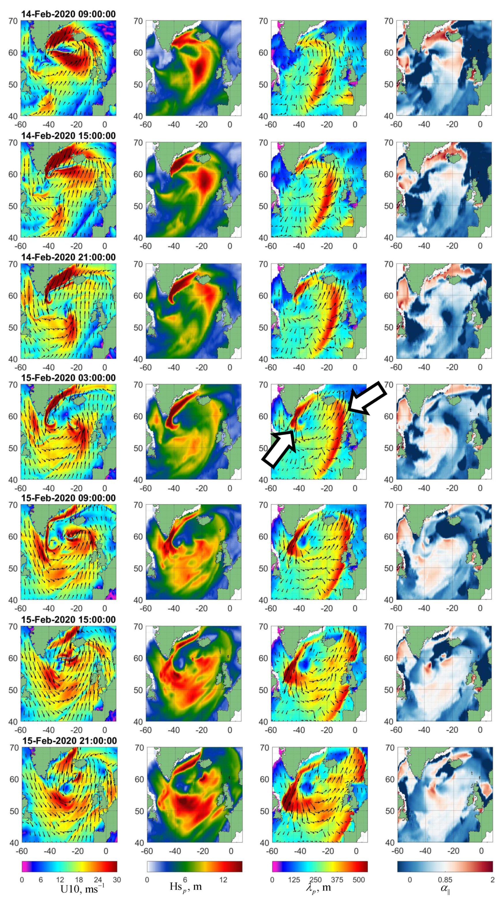
To gain deeper insight into the characteristics of wind wave generation by ETCs, the 6-hourly fields of the surface wave parameters, including H s p , λ p , wave-minus-wind direction ( Δ φ = φ p φ w ), and local inverse wave age ( α | | = u cos ( Δ φ ) / λ g / 2 π ) within the storm area are shown in Figure 2 and Figure 3, for ETC#1 and ETC#2, respectively. All these fields are presented in a moving orthogonal coordinate system with the origin tied to the ETC eye, defined by the minimum of the surface pressure.

3.1. Waves under ETC#1

Modelling the wind wave development starts at the origin of the low pressure area, ending (after eight hours) with the formation of ETC#1 and ETC#2 (see, e.g., Figure 1 from PART I [38]). This allows us to follow the space–time wave development under the ETCs from the very beginning. At the initial stage of ETC#1 evolution, as it moves to the east and acquires a completely cyclonic form, areas with continuous growth of SWH and wavelength are clearly obtained in the right sector of the ETC (Figure 2). Based on inverse wave age fields, waves can be divided into the waves developing under wind, α | | > 0.85 , fully developed, α | | = 0.85 , and swells, α | | < 0.85 . After careful inspection of the inverse wave age maps, in Figure 2, one may find that the development of wind waves begins at the front boundary of the storm area. Since developing waves are slow compared to the ETC’s translation velocity, they move backward relative to the moving ETC in the course of their development. During the first half of ETC#1’s lifespan, fully developed waves ( α | | 0.85 ) with direction aligned to the wind direction ( Δ φ 0 ) can be locally found in the mid of the right sector. In the second half of its lifespan, the area of fully-developed waves is shifted to the rear-right sector. The second and third columns in Figure 2 exhibit clear time growth in SWH and the wavelength of waves generated in the storm area. This fact corresponds to the satellite observations of the linear growth of wave energy in the storm area reported in PART I.
From the maps describing wavelength and direction characteristics, a wave system with λ > 300 m in front of the ETC#1’s forward sector can be easily recognized. The wave direction for this system largely differs from the wind direction. The associated SWHs are much lower than the ETC-generated wave ones. This wave system is not related to ETC#1, and was probably generated prior to ETC#1. Animations 1 and 2 illustrate the origin of this wave system and its evolution.

3.2. Waves under ETC#2

The simulation of ETC#2-generated waves was also considered from the first hours of its formation and is illustrated in Figure 3. The movement direction of ETC#2, shown by red arrows, changes from 30° to 110°, with reference to a trigonometric circle centred in the cyclone’s eye, between the initial hours and the last hours of its life, respectively.
As discussed in PART I, both ETC#1 and ETC#2 are fast-moving atmospheric systems in the sense that their translation velocities are larger than the group velocity of generated wind waves. As a result, the generation of wind waves begins when the front boundary of the storm appears at a given location in the ocean. Then, in the process of their development, the generated waves move backward relative to the ETC, reaching their maximum development at the rear boundary of the storm and, finally, leaving the ETC in the form of swell systems. These peculiar wave developments are clearly exhibited in Figure 3. From the inverse wave age maps shown in the last column, the youngest waves (the largest values of α | | ) are first located along the frontal boundary of the storm. The inverse wave age then gradually decreases towards the storm core, where the developing waves are propagating. Second, similar to the satellite observations (see PART I), the largest value of SWH and wavelength of generated waves are observed in the right and the rear-right sector. This fact suggests that, in the right sector, waves stay under wind forcing for more time than in other sectors. Waves become fully developed, running out of the storm region as swell systems. This finding coincides with the results of self-similar analyses of SWH measurements, discussed in PART I, which confirms the efficiency of the extended fetch/duration mechanism when wind and developing wave directions coincide with the ETC movement direction.
At the last stage of the ETC#2 lifetime, the SWH and wavelength reach 17 m and 500 m, respectively. It corresponds to phenomenal sea conditions, defined by the World Meteorological Organization (WMO) as having an SWH larger than 14 m. A remarkable point is that at the final stage of ETC#2’s lifespan, the waves with H s p > 9 m and λ > 350 m in the rear-left sector occupy a radial range of 300 < r < 1200 km. This indicates the creation of a huge wave front, which can cause a very dangerous situation for marine navigation.
Another interesting feature shown in Figure 3 is the presence of ETC#1’s swell after its lifespan. In the upper-right corner of the wind and wavelength fields, before 13 February 2020 15:00, we see the tail of ETC#1 and the resulting waves. However, there is no sign of ETC#1 in the wind fields after 13 February 2020 15:00. At the same time, swell generated by ETC#1 until 14 February 2020 09:00 is recognized in the lower-right corner of the wavelength fields. These swells can be revealed as a core of locally large λ p , propagating with α | | 0.85 , in the far zone of the forward sector of ETC#2. The area of sudden drop in the inverse wave age values, from α | | 2 to α | | 0 in the forward sector, can be treated as a separation boundary for the waves developing under ETC#2 and swells emitted from other wind systems, including ETC#1.

3.3. Model vs. Observations

Fields of wave parameters and discussion of their characteristics, presented in Section 3.1 and Section 3.2, are based on the outputs of the 2D model. Figure 1, shown in Section 2.3, already demonstrates a “general” validity, over all data covering the North Atlantic during the study period. In this section, more specific satellite sensor tracks, crossing the storm area of ETC#2, were used. Both types of model outputs were considered, namely, the SWH of primary waves system ( H s p ) and the SWH of mixed seas H s T .
Cross sections of H s p and H s T , as a function of latitudes along the altimeter tracks crossing ETC#2, are shown in Figure 4, together with observed SWH, H s o b s . In Figure 4, the geographical location of the tracks is superimposed on the map with wind speed contours and the coloured map of H s T . The altimeter tracks cover various parts of ETC#2, Figure 4. Comparing the H s o b s , H s p , and H s T profiles, a rather good overall consistency is found between model simulations and observations. However, some differences can be notified, e.g., model underestimation of SWH highest values around 15 m at 13:00 and 23:00. On the other hand, after careful inspection, these underestimations, at least at 23:00, are apparently related to the spatial shift of the maximal model values of SWH from the altimeter track. Notice that the model values of H s T and H s p in the storm area of ETC are almost the same, but a bit different outside, where the existence of the mixed seas is likely plausible.

4. Results: Evolution of Swell after the ETC Lifespan

On 14 February 2020 around 09:00, ETC#2 stopped moving to the northeast, changed direction and ceased to exist. Instead, a strong wind jet formed along Greenland at a speed of about 35 ms 1 . This wind jet triggered the generation of a new wind wave system developing along the coast of Greenland, which further radiated into the “open ocean” from Cape Farewell, Figure 5. At the same time, after ETC#2 ceasing, the wind waves which were generated in its storm area continued to evolve as a system of swell waves, traveling northeast, see Figure 5. Both these wave systems, swell emitting from Cape Farewell, and swell traveling northeast from ETC#2, are indicated by arrows in Figure 5. The two systems represent the main subject of investigation in this section, using the spectral information from SWIM off-nadir measurements, synthetic aperture radar (SAR) images, the altimeters observations, and the model outputs.

4.1. Evolution of the Northeastward Swell

Referring to the last row of Figure 3 and the first row of Figure 5, a front of waves is observed on 14 February 2020 morning, with λ 300 m, H s 10 m, and α | | 0.85 . These waves occupy a very large area in the rear-left sector of ETC#2 (see last row of Figure 3). Travelling eastward, this wave front can reach the Celtic Sea and subarctic seas, such as the Norwegian Sea. In Figure 6, the spatio-temporal evolution of this front is illustrated at times, when the SWIM tracks crosses part of the front. First row of Figure 6 is associated with the final moments of ETC#2 life, shown in the last two rows of Figure 3. The SWIM tracks are superimposed on the synchronous field of SWH and the wavelength is obtained from the 2D model.
Going forward in time (from up to down rows of Figure 5 and Figure 6), the east–northeastward propagation of this wave front is easily recognisable. The measurements of SWH, λ p , and φ p also confirm this front propagation. Based on simulations and measurements, following Figure 6, the spatio-temporal evolution of swell in the eastern side of the North Atlantic Ocean is thus found to influence the European coasts and subarctic seas for a long time after the disappearance of ETC#2. On the maps, Figure 6, the maximal SWH levels decrease from about 17 m on 14 February 2020 09:00 to 8 m on 15 February 2020 20:00, following energy dissipation, while the maximal wavelength is >450 m.
The 2D wavenumber spectra derived from SWIM data in the area of wind waves (box I in the first row of Figure 6) and in the area of swell front (box II in the third row of Figure 6) are shown in Figure 7. The SWIM wave spectra were taken from the IFREMER database (ftp.ifremer.fr, accessed on 20 March 2022). The second column of Figure 7 displays the omnidirectional spectra S ( k ) , scaled by e / k p , i.e., k p S ( k ) / e , as a function of k / k p , where e is the energy (integral of S over k) and k p is the spectral peak wavenumber. The green lines show the JONSWAP [41] spectra with similar scaling. The measured spectrum for the the wind waves is very similar to the empirical JONSWAP one, except for some differences in the slope of the spectral tail. In the swell front area, a combination of a dominant swell system and much shorter wind waves can be revealed. The presence of wind waves noticeably changes the omnidirectional spectrum due to the addition of energy in the tail of the spectrum, at frequencies above the peak frequency of the wind waves. Nevertheless, shape of the scaled total spectrum (where swell dominates) is again surprisingly close to that of the JONSWAP spectrum. This observation is similar to what was reported by [42,43] under hurricane conditions; the shape of the dominant wave spectra, regardless of whether they are wind waves or swells, is very close to the shape of the JONSWAP spectrum.
Histograms of the model energy distributions of wave-trains over wavelength and directions shown in the third column serve as a good proxy for 2D spectra. Comparing the first and third columns in Figure 7, model spectral distributions of wave-trains are indeed found to be consistent with the measured 2D spectra. The travel time histogram (last column) gives an idea of the history of wave packets (wind driven and swell) forming a wave pattern at a given time and at a given point.
Figure 8 shows time evolution of the peak wavelength (SWIM data) and energy collected from all the altimeter tracks crossing the swell front traveling northeastward. The time count starts from 14 February 2020 09:00, which is considered the end of the life of ETC#2. Although the wavelength measurements by SWIM are very limited, they nevertheless demonstrate expected stationary behaviour or slow growth, as predicted by the 2D model. In contrast, the energy of the swell at the front, measured by altimeters, decreases rather quickly. After 40 h of travel (which is equivalent to a distance of about 2000 km), the energy drops by about four times. This observed energy decay is consistent with model simulations of the total wave energy, co-located with altimeter measurements (open circles), with maximal values at the part of swell front which moves northeastward.
The red dashed curve in Figure 8 shows swell energy attenuation due to the divergence of wave-rays which reads:
e / e 0 = 1 + c g G n 0 t 1 ,
where G n 0 is the initial value of cross-ray gradient of swell direction. Relationship (5) represents a straightforward solution of Equation (1), for which the effect of the energy source S e on swell evolution is ignored, with the swell wavelength kept constant. A full solution for swell energy and wavelength evolution due to the effect of dissipation, non-linear waves interactions and wave-rays convergence/divergence can be found in [35,36]. Here, we considered only the effect of wave-ray divergence, which seems to be the governing mechanism. The initial value of the cross-ray gradient in Equation (5) can be evaluated as G n 0 = 1 / R f with R f the radius of the swell front curvature. The red dashed curve shown in Figure 8 corresponds to R f = 500 km, which is about the radius of ETC#2. The observed attenuation of swell energy, e t 1 , is remarkably faster than that predicted by the effect of the swell energy dissipation in [33]: e t 1 / 2 , by non-linear wave–wave interactions in [44]: e t 1 / 3 , and that reported by [12] due to the interaction of swell with the airflow.

4.2. Southward Swell

According to the wind fields in Figure 5, a strong wind jet formed along Greenland at a speed of about 35 ms 1 . This wind jet resulted from the deformation of the frontal part of ETC#2. It provided more than 1200 km of fetch length for wave development over a period of more than 12 h. The waves, which were developing in the frontal part of ETC#2, becoming fully developed, reached a phenomenal SWH and wavelength of 18 m and 600 m, respectively, and consequently further propagated as swell. Although the wind field in the basin became quite complex, this wave front further radiated into the “open ocean” from Cape Farewell, which is clearly visible in Figure 5.
Some fragments illustrating the development of the wave system along the Greenland coast, leading to the formation of the radiated swell, were captured with SWIM measurements, shown in Figure 9. Model simulations of H s , λ p and φ p are consistent with these measurements, suggesting the model’s capability of realistically reproducing the wave development and swell evolution. Referring to Figure 5 and Figure 9, the swell front, associated with λ p > 500 m and H s > 13 m, originating on 14 February 2020 21:00 at a latitude of 56°N can be easy identified. This swell front then further moved southward, achieving 48°N on 15 February 2020 21:00 (see inverse wave age and wavelength plots on the fore-said dates in Figure 5).
An SAR image in HH-polarisation from https://sentinel.esa.int/ (Sentinel-1B, accessed on 20 February 2022) acquired over Cape Farewell on 14 February 2020 evening, when the swell front was reaching the open ocean, shown in Figure 10a. To derive distributions of wavelength/direction of waves over this SAR scene, we applied Fast Fourier Transform (FFT) to each of the image boxes with a size of 256 × 256 pixels (e.g., Figure 10b,d), which were spread over the whole SAR image, to obtain a 2D wavenumber ( k x , k y ) image spectra; two examples are demonstrated in Figure 10c,e. The spectral level of the SAR image can potentially be converted to the wave elevation spectrum, but this procedure is not straightforward, and we leave this issue out of the scope of this paper. Instead, focusing on wave kinematics, we considered only the SAR detected wavelength and direction. In order to remove ambiguity, we used the wave direction from the 2D model outputs.
The resulting field of wavenumber vectors derived from the SAR image is shown in Figure 11a. This field exhibits a spectacular swell front moving southward, over which the wavelength rapidly changes from 500 m to 250 m. In addition, the existence of the western boundary of the swell was confirmed by synchronous SWIM measurements shown in the same figure. Additionally, SWIM measurements a day later, see Figure 9 bottom row, revealed a similar rapid drop of the spectral peak wavelength and SWH over this swell front; however, it had already shifted southward. The model field of the swell front, see Figure 11b, is consistent, in general, with the measurements, providing a similar change of wavelengths over the front and its location. However, the existence of an area filled with “shorter” waves in the eastern part of the model scene (coinciding with the low-wind speed area) is not confirmed by the measurements.
SWIM-derived 2D wavenumber spectra on a different side of the swell front (box III and box IV in the last row of Figure 9) are shown in Figure 12. The spectrum inside the swell area, illustrated in the first row of Figure 12, displays the superposition of the dominant swell system and the system of shorter wind waves. The spectrum outside the swell front exhibits a wave system of remarkably shorter waves (as compared with swell in box III) with a wide angular spread. Similar to the case with northeast swell, the scaled omnidirectional spectra, k p S ( k ) / e , on different sides of the swell front are very similar and consistent with the shape of the scaled JONSWAP spectrum, again confirming the experimental finding by [42,43] for waves in hurricanes. The histograms of distribution of the model energy of wave-trains over wavelength and directions, shown in the third column of Figure 12, are also consistent with 2D SWIM spectra. The travel time histogram (last column) gives the history of wave packets (wind driven and swell) forming a wave pattern at a given time and at a given point.

5. In Situ Data

In situ buoy measurements complement the description of waves generated by ETCs, to perform additional validation of the proposed model. The hourly time series of wind speed at height 1 m, significant wave height (SWH), and wave period (equal to average zero crossing period) measurements taken from the buoy “NO TS MO 6400045” located between Iceland and Ireland, on 11.4°W and 59.1°N for the period from 11 February 12:00 to 15 February 23:00, 2020, are shown in Figure 13. Note that, to be consistent with SWIM data, we further used λ z instead of T z which is calculated using the dispersion relation, λ z = g T z 2 / ( 2 π ) , which is shown in Figure 13c instead of T z . For additional comparison, the NCEP/CFSv2 10-m wind speed and model SWH and wave frequency (wavelength via the dispersion relation) at the buoy location were also plotted.
To compare in situ measurements with model estimates, the measured average zero crossing period of wave, T z (or equivalent frequency ω z = 2 π / T z ), was converted to the spectral peak period (frequency, ω p ). Following [45], ω z is expressed through the spectral moments as:
ω z 2 = m 2 m 0 = ω 2 F ( ω ) d ω F ( ω ) d ω ,
where the m j is the jth moment of the wave elevation spectrum F ( ω ) . As found, the shape of the observed wave spectra is very similar to the JONSAWAP spectrum [46], see Figure 7 and Figure 12. In this case, the link between ω z and ω p can be found by substituting the JONSWAP spectrum in (6), leading to ω z = 1.3 ω p . Following this, an estimate of the spectral peak wavelength based on the buoy measurements of wave period (frequency ω z ) is λ p = 1 . 3 2 2 π g / ω z 2 .
Due to its location, the buoy should record the passage of ETC#2-generated waves from the North Atlantic to the subarctic seas, similar to what follows from the model simulations in Animation 3. Following Figure 13a, a wind speed of u 10 26 ms 1 was recorded on 14 February 2020 03:00 and 14 February 2020 12:00 that, according to Animation 3, corresponded to the passage of the right section of ETC#2 through the buoy location. Going back in time from 14 February 2020 03:00, the wind speed increase began on 13 February 2020 16:00. However, the increase for SWH and wavelength occurred about 8 h later. As Animation 3 shows, the growth of SWH and λ on 14 February 2020 00:00 is associated with the swell front radiating out from ETC#2, which resulted in maximal values observed between 14 February 2020 18:00 and 15 February 2020 06:00. According to the evolution of wave characteristics from 14 February 2020 00:00 to 15 February 2020 12:00, one may find that the swells produced by ETC#2 took 36 h to pass the location of the buoy. Nevertheless, the high wind related to ETC#2 passed the buoy location earlier (during 13 February 2020 18:00 and 14 February 2020 20:00) and in a shorter time.
Buoy measurements of wave parameters thus well support the satellite data and further confirm the model’s validity. The synergistic use of multi-sensor satellite and in situ measurements of wave parameters and modelling can thus provide a very detailed and consistent description of the wave field generated by fast moving cyclones both in the inner storm area and for radiating the swell system to the far zone after the ETC passage and dissipation.

6. Conclusions

With these two companion papers, we thoroughly investigated the main characteristics of the phenomenal sea state generated by fast-moving ETCs in the North Atlantic. We demonstrated that a suite of data from different sources—a combination that may not be typical in forecasting environments—can give a remarkably coherent characterisation of an extreme storm event and associated wave fields. The present study indeed combined multi-satellite and in situ observations, with simplified 1D and 2D parametric models which conceptually follow self-similarity principles to quantify wave developments.
Simulations were performed to describe the spatio-temporal evolution of surface wave fields in the North Atlantic, spanning 7 days from 9 00:00 UTC to 15 23:00 UTC, February, 2020. In total, 130 altimeter tracks crossed the computational domain during this period. A rather high level of correlation between the model and the measured SWH (correlation coefficient is about 0.87) was found, justifying the use of the proposed simplified model framework to describe wave properties generated by ETCs.
The selected ETCs were fast-moving storms, for which the resonance (synchronism) between group velocities of generated waves and the ETC translation velocity was impossible. Satellite observations and model simulations confirm that the ETC storm areas are indeed filled with wind-developing waves, with wave generation starting when the front-boundary of the storm crosses a given location in the ocean.
In the course of their development, wind waves move backward relative to the storm and grow in time under the strong wind forcing. Waves then attain maximal development (maximal values of SWH up to 17 m and wavelengths up to 500 m) in the rear-right ETC sectors. Spatial distributions of observed and simulated wave fields in the inner storm area of ETC are thus remarkably different from those generally associated with a TC, where waves are usually enhanced in the right-front sector.
The fast-moving nature of the ETCs further leads to the formation of swell systems, generated from the rear-right sector and trailing behind the ETC. At the precise time the ETC#2 ceased, the swell SWH and its wavelength attained abnormal phenomenal values of 17 m and 450 m, respectively. This swell front then propagated over the eastern part of the North Atlantic and the Norwegian sea. Satellite observations of the evolution of this swell front (during 40 h or at a distance of about 2000 km) confirmed that the swell wavelength remained practically unchanged, while the swell SWH attenuated gradually with the distance. Waves thus closely follow principles of geometrical optics, with a constant wave period along geodesics, when following a wave packet at the group speed [14,16]. Yet, close to their source point, initially steep swell systems rapidly attenuate. Observed estimates of the swell energy attenuation were found to be proportional to the inverse travel distance. Such a decay remarkably exceeds model estimates predicted by the wave energy dissipation and/or non-linear wave–wave interactions mechanisms. This non-linear behaviour may possibly be postulated to trace the transition from a laminar to a turbulent air-side boundary layer [12]. However, in the present study, observed attenuation of swell energy appeared to be more consistently explained by the effect of wave-ray divergence caused by the initial curvature of the swell front [47].
Another spectacular wave field feature related to ETC#2 (more precisely when it ceases) is the generation of abnormally high waves in the Greenland coastal region. These waves are caused by the ETC#2 transformation to become an along-coastal wind jet. This jet occurred as part of newly-formed Icelandic lows, following the end of ETC#2. According to the satellite observations and model results, sea state parameters in this local high-wind-speed region also reached very high values—an SWH of 18 m and a wavelength of about 600 m.
At the southern tip of Greenland (Cape Farewell), these huge waves turned into a swell system that moved southward to the open ocean. Satellite measurements and model simulations captured the swell front and its southward motion, also displaying large wavelength changes over the swell front, i.e., from 600 m to 250 m.
We are certainly encouraged by these results, reporting our ability to both model and observe extreme wave events. The proposed analysis framework shall now provide an improved understanding of spatio-temporal storm characteristics for extra-tropical swell systems, and may not only help to identify biases in swell forecast models but also help improve air-sea fluxes and upper-ocean mixing estimations.

Author Contributions

Conceptualization, V.K. and B.C.; Methodology, V.C.S., V.K., M.Y., F.C. and B.C.; Software, V.C.S.; Validation, V.C.S. and F.C.; Formal analysis, V.C.S., V.K., M.Y. and B.C.; Investigation, F.C.; Writing—original draft, V.C.S.; Writing—review & editing, V.K., M.Y. and B.C.; Visualization, V.C.S.; Supervision, V.K.; Project administration, V.K. All authors have read and agreed to the published version of the manuscript.

Funding

The core support for this work was provided by the Russian Science Foundation through Project No. 21-47-00038. The support of the Ministry of Science and Education of the Russian Federation under State Assignment No. FNNN-2021-0004 at MHI RAS and State Assignment No. 0763-2020-0005 at RSHU is gratefully acknowledged.

Data Availability Statement

The data supporting reported results are extracted as following: Sentinel-3A and B https://finder.creodias.eu (accessed on 20 March 2022); AltiKa and JASON-3 and SWIM l2 products https://aviso-data-center.cnes.fr (accessed on 20 March 2022); CryoSat-2 ftp://science-pds.cryosat.esa.int (accessed on 20 March 2022); SWIM l2s products ftp://ftp.ifremer.fr (accessed on 20 March 2022); NCEP/CFSv2 https://rda.ucar.edu/ (accessed on 20 March 2022); Sentinel-1B SAR images https://sentinel.esa.int/ (accessed on 20 February 2022); observations at buoy “NO TS MO 6400045” https://data.marine.copernicus.eu/ (accessed on 8 June 2022); ice concentration https://seaice.uni-bremen.de/ (accessed on 12 August 2022). The simulation results, obtained from the 2D model are presented on Animation 1 and Animation 2.

Acknowledgments

CFOSAT-SWIM measurements were provided by IFREMER Wind and Wave Operational Center (IWWOC), co-funded by CNES and IFREMER. NCEP/CFSv2 data provided by the OAA/OAR/ESRL PSD, Boulder, CO, USA, from their Web site at NCEP/CFSv2 website. We also acknowledge the ESA MAXSS Project 4000132954/20/I-NB.

Conflicts of Interest

The authors declare no conflict of interest.

Abbreviations

The following abbreviations are used in this manuscript:
1D, 2D and 3DOne, two and three Dimensional
SWH/HsSignificant Wave Height
ETCExtra-Tropical Cyclone
TCTropical Cyclone
CFOSATChinese-French Oceanographic Satellite
SWIMSurface Wave Exploration and Monitoring
NCEPNational Centers for Environmental Prediction
CFSv2Climate Forecast System Version 2
IFREMERInstitut Français de Recherche pour l’Exploitation de la Mer,
French Research Institute for Exploitation of the Sea
JONSWAPJoint North Sea Wave Project
SARSynthetic Aperture Radar
FFTFast Fourier Transformation
NBINormalized Bias
WMOWorld Meteorological Organization

References

  1. Hewson, T.D.; Neu, U. Cyclones, windstorms and the IMILAST project. Tellus A Dyn. Meteorol. Oceanogr. 2015, 67, 27128. [Google Scholar] [CrossRef]
  2. Ponce de León, S.; Bettencourt, J. Composite analysis of North Atlantic extra-tropical cyclone waves from satellite altimetry observations. Adv. Space Res. 2021, 68, 762–772. [Google Scholar] [CrossRef]
  3. Hanafin, J.A.; Quilfen, Y.; Ardhuin, F.; Sienkiewicz, J.; Queffeulou, P.; Obrebski, M.; Chapron, B.; Reul, N.; Collard, F.; Corman, D.; et al. Phenomenal Sea States and Swell from a North Atlantic Storm in February 2011: A Comprehensive Analysis. Bull. Am. Meteorol. Soc. 2012, 93, 1825–1832. [Google Scholar] [CrossRef]
  4. de León, S.P.; Soares, C.G. Extreme wave parameters under North Atlantic extratropical cyclones. Ocean Model. 2014, 81, 78–88. [Google Scholar] [CrossRef]
  5. Kita, Y.; Waseda, T.; Webb, A. Development of waves under explosive cyclones in the Northwestern Pacific. Ocean Dyn. 2018, 68, 1403–1418. [Google Scholar] [CrossRef]
  6. Hell, M.C.; Ayet, A.; Chapron, B. Swell Generation under Extra-Tropical Storms. J. Geophys. Res. Oceans 2021, 126, e2021JC017637. [Google Scholar] [CrossRef]
  7. Enríquez, A.R.; Marcos, M.; Álvarez-Ellacuría, A.; Orfila, A.; Gomis, D. Changes in beach shoreline due to sea level rise and waves under climate change scenarios: Application to the Balearic Islands (western Mediterranean). Nat. Hazards Earth Syst. Sci. 2017, 17, 1075–1089. [Google Scholar] [CrossRef]
  8. Ferreira, Ó. Storm groups versus extreme single storms: Predicted erosion and management consequences. J. Coast. Res. 2005, 221–227. Available online: http://www.jstor.org/stable/25736987 (accessed on 20 March 2022).
  9. Hunt, I.A. Design of Sea-Walls and Breakwaters. Trans. Am. Soc. Civ. Eng. 1961, 126, 542–570. [Google Scholar] [CrossRef]
  10. Morison, M.L.; Imberger, J. Water-Level Oscillations in Esperance Harbour. J. Waterw. Port Coast. Ocean Eng. 1992, 118, 352–367. [Google Scholar] [CrossRef]
  11. Russell, P.E. Mechanisms for beach erosion during storms. Cont. Shelf Res. 1993, 13, 1243–1265. [Google Scholar] [CrossRef]
  12. Ardhuin, F.; Chapron, B.; Collard, F. Observation of swell dissipation across oceans. Geophys. Res. Lett. 2009, 36, 37030. [Google Scholar] [CrossRef]
  13. Munk, W.; Snodgrass, F. Measurements of southern swell at Guadalupe Island. Deep Sea Res. 1957, 4, 272–286. [Google Scholar] [CrossRef]
  14. Snodgrass, F.E.; Hasselmann, K.F.; Miller, G.R.; Munk, W.H.; Powers, W.H.; Deacon, G.E.R. Propagation of ocean swell across the Pacific. Philos. Trans. R. Soc. Lond. Ser. A Math. Phys. Eng. Sci. 1966, 259, 431–497. [Google Scholar] [CrossRef]
  15. Chapron, B.; Johnsen, H.; Garello, R. Wave and wind retrieval from sar images of the ocean. Ann. Des Télécommun. 2001, 56, 682–699. [Google Scholar] [CrossRef]
  16. Collard, F.; Ardhuin, F.; Chapron, B. Monitoring and analysis of ocean swell fields from space: New methods for routine observations. J. Geophys. Res. 2009, 114, C07023. [Google Scholar] [CrossRef]
  17. Hauser, D.; Tourain, C.; Hermozo, L.; Alraddawi, D.; Aouf, L.; Chapron, B.; Dalphinet, A.; Delaye, L.; Dalila, M.; Dormy, E.; et al. New Observations From the SWIM Radar On-Board CFOSAT: Instrument Validation and Ocean Wave Measurement Assessment. IEEE Trans. Geosci. Remote Sens. 2021, 59, 5–26. [Google Scholar] [CrossRef]
  18. Aouf, L.; Wang, J.; Hauser, D.; Chapron, B.; Tourain, C. On the Assimilation of Wide Swath Significant Wave Height and Directional Wave Observations in Wave Model: Perspective for Operational Use. In Proceedings of the IGARSS 2022—2022 IEEE International Geoscience and Remote Sensing Symposium, Kuala Lumpur, Malaysia, 17–22 July 2022; pp. 6772–6774. [Google Scholar] [CrossRef]
  19. Tolman, H.L. User Manual and System Documentation of WAVEWATCH III TM Version 3.14; Technical Note No. 276; MMAB Contribution; U.S. Department of Commerce: Camp Springs, MD, USA, 2009.
  20. Group, T.W. The WAM Model—A Third Generation Ocean Wave Prediction Model. J. Phys. Oceanogr. 1988, 18, 1775–1810. [Google Scholar] [CrossRef]
  21. Booij, N.; Ris, R.C.; Holthuijsen, L.H. A third-generation wave model for coastal regions: 1. Model description and validation. J. Geophys. Res. 1999, 104, 7649–7666. [Google Scholar] [CrossRef]
  22. Kalourazi, M.Y.; Siadatmousavi, S.M.; Yeganeh-Bakhtiary, A.; Jose, F. WAVEWATCH-III source terms evaluation for optimizing hurricane wave modeling: A case study of Hurricane Ivan. Oceanologia 2021, 63, 194–213. [Google Scholar] [CrossRef]
  23. Durrant, T.H.; Greenslade, D.J.; Simmonds, I. The effect of statistical wind corrections on global wave forecasts. Ocean Model. 2013, 70, 116–131. [Google Scholar] [CrossRef]
  24. Feng, H.; Vandemark, D.; Quilfen, Y.; Chapron, B.; Beckley, B. Assessment of wind-forcing impact on a global wind-wave model using the TOPEX altimeter. Ocean Eng. 2006, 33, 1431–1461. [Google Scholar] [CrossRef]
  25. Janssen, P.A.; Bidlot, J.R. Progress in Operational Wave Forecasting. Procedia IUTAM 2018, 26, 14–29. [Google Scholar] [CrossRef]
  26. Ponce, S.; Ocampo-Torres, F.J. Sensitivity of a wave model to wind variability. J. Geophys. Res. 1998, 103, 3179–3201. [Google Scholar] [CrossRef]
  27. Stopa, J.E.; Cheung, K.F. Intercomparison of wind and wave data from the ECMWF Reanalysis Interim and the NCEP Climate Forecast System Reanalysis. Ocean Model. 2014, 75, 65–83. [Google Scholar] [CrossRef]
  28. Abdolali, A.; Roland, A.; van der Westhuysen, A.; Meixner, J.; Chawla, A.; Hesser, T.J.; Smith, J.M.; Sikiric, M.D. Large-scale hurricane modeling using domain decomposition parallelization and implicit scheme implemented in WAVEWATCH III wave model. Coast. Eng. 2020, 157, 103656. [Google Scholar] [CrossRef]
  29. Babanin, A.V.; Rogers, W.E.; de Camargo, R.; Doble, M.; Durrant, T.; Filchuk, K.; Ewans, K.; Hemer, M.; Janssen, T.; Kelly-Gerreyn, B.; et al. Waves and Swells in High Wind and Extreme Fetches, Measurements in the Southern Ocean. Front. Mar. Sci. 2019, 6, 361. [Google Scholar] [CrossRef]
  30. Hasselmann, K.; Sell, W.; Ross, D.B.; Müller, P. A Parametric Wave Prediction Model. J. Phys. Oceanogr. 1976, 6, 200–228. [Google Scholar] [CrossRef]
  31. Gunther, H.; Rosenthal, W.; Weare, T.J.; Worthington, B.A.; Hasselmann, K.; Ewing, J.A. A hybrid parametrical wave prediction model. J. Geophys. Res. 1979, 84, 5727–5738. [Google Scholar] [CrossRef]
  32. Kitaigorodskii, S. Application of the theory of similarity to the analysis of wind-generated wave motion as a stochastic process. Izv. Geophys. Ser. Acad. Sci. USSR 1962, 1, 105–117. [Google Scholar]
  33. Kudryavtsev, V.; Yurovskaya, M.; Chapron, B. 2D Parametric Model for Surface Wave Development under Varying Wind Field in Space and Time. J. Geophys. Res. Oceans 2021, 126, e2020JC016915. [Google Scholar] [CrossRef]
  34. Kudryavtsev, V.; Yurovskaya, M.; Chapron, B. Self-Similarity of Surface Wave Developments under Tropical Cyclones. J. Geophys. Res. Oceans 2021, 126, e2020JC016916. [Google Scholar] [CrossRef]
  35. Yurovskaya, M.; Kudryavtsev, V.; Mironov, A.; Mouche, A.; Collard, F.; Chapron, B. Surface Wave Developments under Tropical Cyclone Goni (2020): Multi-Satellite Observations and Parametric Model Comparisons. Remote Sens. 2022, 14, 2032. [Google Scholar] [CrossRef]
  36. Yurovskaya, M.; Kudryavtsev, V.; Chapron, B. A self-similar description of the wave fields generated by tropical cyclones. Ocean Model. 2023, 183, 102184. [Google Scholar] [CrossRef]
  37. Kudryavtsev, V.; Cheshm Siyahi, V.; Yurovskaya, M.; Chapron, B. On Surface Waves in Arctic Seas. Bound.-Layer Meteorol. 2022. [Google Scholar] [CrossRef]
  38. Cheshm Siyahi, V.; Kudryavtsev, V.; Yurovskaya, M.; Collard, F.; Chapron, B. On Surface Waves Generated by Extra-Tropical Cyclones—Part I: Multi-Satellite Measurements. Remote Sens. 2023, 15, 1940. [Google Scholar] [CrossRef]
  39. Saha, S.; Moorthi, S.; Wu, X.; Wang, J.; Nadiga, S.; Tripp, P.; Behringer, D.; Hou, Y.T.; Chuang, H.Y.; Iredell, M.; et al. NCEP Climate Forecast System Version 2 (CFSv2) Selected Hourly Time-Series Products; Research Data Archive at the National Center for Atmospheric Research, Computational and Information Systems Laboratory: Boulder, CO, USA, 2011. [Google Scholar] [CrossRef]
  40. Hanna, S.R.; Heinold, D.W. Simple Statistical Methods for Comparative Evaluation of Air Quality Models. In Air Pollution Modeling and Its Application V; De Wispelaere, C., Schiermeier, F.A., Gillani, N.V., Eds.; Springer: Boston, MA, USA, 1986; pp. 441–452. [Google Scholar] [CrossRef]
  41. Donelan, M.A.; Hamilton, J.; Hui, W.H.; Stewart, R.W. Directional spectra of wind-generated ocean waves. Philos. Trans. R. Soc. Lond. Ser. A Math. Phys. Eng. Sci. 1985, 315, 509–562. [Google Scholar] [CrossRef]
  42. Young, I.R. Directional spectra of hurricane wind waves. J. Geophys. Res. 2006, 111, C08020. [Google Scholar] [CrossRef]
  43. Le Merle, E.; Hauser, D.; Yang, C. Wave Field Properties in Tropical Cyclones from the Spectral Observation of the CFOSAT/SWIM Spaceborne Instrument. J. Geophys. Res. Oceans 2023, 128, e2022JC019074. [Google Scholar] [CrossRef]
  44. Badulin, S.I.; Zakharov, V.E. Ocean swell within the kinetic equation for water waves. Nonlinear Process. Geophys. 2017, 24, 237–253. [Google Scholar] [CrossRef]
  45. Cartwright, D.E.; Longuet-Higgins, M.S. The statistical distribution of the maxima of a random function. Proc. R. Soc. Lond. Ser. A Math. Phys. Eng. Sci. 1956, 237, 212–232. [Google Scholar] [CrossRef]
  46. Hasselmann, K.; Barnett, T.P.; Bouws, E.; Carlson, H.; Cartwright, D.E.; Enke, K.; Ewing, J.; Gienapp, A.; Hasselmann, D.; Kruseman, P.; et al. Measurements of wind-wave growth and swell decay during the Joint North Sea Wave Project (JONSWAP). Ergaenzungsheft Dtsch. Hydrogr. Z. Reihe A 1973. Available online: https://hdl.handle.net/21.11116/0000-0007-DD3C-E (accessed on 20 March 2022).
  47. Delpey, M.T.; Ardhuin, F.; Collard, F.; Chapron, B. Space-time structure of long ocean swell fields. J. Geophys. Res. 2010, 115, C12037. [Google Scholar] [CrossRef]
Figure 1. Comparison of measured and modelled H s T vs. H s o b s (a), λ p (b) and φ (c) with normalised bias (NBI), normalised root-mean-square error (HH) and correlation coefficient (R). The comparisons were accomplished for the period of 11–15 February 2020 in the region 30°N–38°N 75°W–20°E.
Remotesensing 15 02377 g001
Figure 2. Six-hour fields of the wind velocity and the model wave parameters in a moving orthogonal coordinate system with the origin at the eye of ETC#1. Columns from left to right: wind field, significant wave height ( H s p ), wavelength ( λ p ), and wave direction ( φ p ), wave-wind directions difference ( Δ φ = φ p φ w ), and local inverse wave age ( α | | = u cos ( φ p φ w ) / c p ). The red arrow in the centre of each panel indicates the movement direction of ETC#1. Circle radii start at 200 km in 200 km increments.
Remotesensing 15 02377 g002
Figure 3. The same as Figure 2, but for ETC#2.
Remotesensing 15 02377 g003
Figure 4. The modelled vs. measured profiles of SWH. First and third rows: altimeter tracks superimposed on maps of wind speed (contour lines) and model SWH, H s T (colour) for ETC#2. Second and fourth rows: cross section of H s o b s (black curves), H s p (blue curves), and H s T (red curves) along the altimeter tracks as a function of latitude.
Remotesensing 15 02377 g004
Figure 5. Six-hour fields of the wind velocity and the model wave parameters in geographical coordinates after cessation of ETC#2. Columns from left to right: wind velocity, significant wave height ( H s p ), wavelength ( λ p ), wave direction ( φ p ), and local inverse wave age ( α | | = u cos ( φ p φ w ) / c p ). Two white arrows indicate the two swell fronts considered in the text.
Remotesensing 15 02377 g005
Figure 6. Spatio-temporal evolution of waves, after disappearance of ETC#2, when the CFOSAT-SWIM tracks cross eastward moving swell front. Columns from left to right: geographical location of SWIM tracks superimposed on colour-maps of modelled λ p , where the arrows show φ p ; cross section of λ p o b s (black circles) and λ p (blue asterisks); cross section of φ p o b s (black circles) and φ p (blue asterisks); SWIM nadir tracks superimposed on colour-maps of modelled H s T ; cross section of H s o b s (black curves) and modelled H s T (blue curves).
Remotesensing 15 02377 g006
Figure 7. Two-dimensional (2D) directional wave spectra derived from SWIM inside boxes I and II. Locations of these boxes are shown in the first and third rows of Figure 6 (left columns). The second column: scaled omnidirectional spectra, k p S ( k ) / e , (red circles) as a function of k / k p compared to scaled JONSWAP spectra (green curves). The third and fourth columns are model histograms of SWH and travel time distributions over wavelength and directions; purple arrow indicates wind direction.
Remotesensing 15 02377 g007
Figure 8. (a) Time evolution of swell energy: red circles are altimeter measurements, open circles are the model values at the point of the measurements, black curve shows maximal values of the model energy at the front, the red dashed curve is obtained from (5) with G n 0 = 1 / 500   km . (b) Time evolution of swell wavelength: red points are SWIM measurements, black curve is the model.
Remotesensing 15 02377 g008
Figure 9. The same as Figure 6, but when the CFOSAT-SWIM tracks cross the southward radiating swell front.
Remotesensing 15 02377 g009
Figure 10. (a) Sentinel-1B Synthetic aperture radar (SAR) image on HH polarisation on 14 February 2020 evening in the south of Greenland. (b,d) zoom on SAR image for areas indicated by red and blue boxes in (a). (c,e) are the SAR image wavenumber ( k x , k y ) spectra of (b,d) zooms. The circles in (c,e) indicate the wavelength, λ = 2 π / k , with radii start at 200 m (the biggest circle) in 100 m increment.
Remotesensing 15 02377 g010
Figure 11. (a) Spatial distributions of dominant wavelengths (color) and directions (arrows) derived from the SAR image shown in Figure 11a, with the SWIM off-nadir measurements of λ p and φ p . (b) The model fields of wavelength (color) and directions (arrows) of primary wave system; white lines indicate the contour of SAR image.
Remotesensing 15 02377 g011
Figure 12. The same as Figure 7 but for boxes III and IV indicated in Figure 9.
Remotesensing 15 02377 g012
Figure 13. (a) Wind speed, (b) significant wave height, (c) wavelength at location of buoy “NO TS MO 6400045”. The designation of the lines is given in the legends to the plots. Buoy wavelength, λ z = g T z 2 / ( 2 π ) , is derived from the measured wave period T z using the dispersion relation, and buoy-peak-wavelength is λ p = 1 . 3 2 λ z . Wind speed on 10-m height is derived from the measured wind speed (1-m height) using the logarithmic wind profile with C D 10 = 0.0015 . The animation, which shows the waves passing the buoy location, can be found in Animation 3.
Remotesensing 15 02377 g013
Disclaimer/Publisher’s Note: The statements, opinions and data contained in all publications are solely those of the individual author(s) and contributor(s) and not of MDPI and/or the editor(s). MDPI and/or the editor(s) disclaim responsibility for any injury to people or property resulting from any ideas, methods, instructions or products referred to in the content.

