BSFCDet: Bidirectional Spatial–Semantic Fusion Network Coupled with Channel Attention for Object Detection in Satellite Images

Abstract

Due to the increasing maturity of deep learning and remote sensing technology, the performance of object detection in satellite images has significantly improved and plays an important role in military reconnaissance, urban planning, and agricultural monitoring. However, satellite images have challenges such as small objects, multiscale objects, and complex backgrounds. To solve these problems, a lightweight object detection model named BSFCDet is proposed. First, fast spatial pyramid pooling (SPPF-G) is designed for feature fusion to enrich the spatial information of small targets. Second, a three-layer bidirectional feature pyramid network (BiFPN-G) is suggested to integrate the deep feature’s semantic information with the shallow feature’s spatial information, thus improving the scale adaptability of the model. Third, a novel efficient channel attention (ECAM) is proposed to reduce background interference. Last, a new residual block (Resblock_M) is constructed to balance accuracy and speed. BSFCDet achieves high detection performance while satisfying real-time performance, according to experimental results.

1. Introduction

Remote sensing technology refers to technology that collects electromagnetic radiation information on Earth objects via aviation, aerospace, or artificial satellites and recognizes the Earth’s environment and resources. Due to the increasing maturity of the aviation industry, the count and quality of remote sensing images (RSIs) have improved significantly, and it is important to explore how to obtain and utilize the information in RSIs [1]. Remote sensing object detection (RSOD) is a popular study interest in RSI processing, with the aim of identifying the categories of objects of interest in RSIs and detecting the locations of objects [2]. Compared to natural scene images, RSIs have higher resolution, wider coverage, and contain more information. Based on the above advantages, RSOD is widely utilized in the following fields:

• In military reconnaissance, RSOD techniques can detect aircraft, missiles, and other military equipment and facilities, which is convenient for the rapid acquisition of military intelligence and is an important part of the modern military system.
• In urban planning, the relevant departments use RSOD techniques to quickly obtain urban topography, traffic conditions, and other data, which is conducive to the coordination of urban spatial layouts and the rational use of urban land.
• In agricultural monitoring, RSOD techniques are used to monitor crop growth, pests, and other information to take preventive measures to reduce economic losses.

Due to the increasing maturity of deep learning, the performance of RSOD has significantly improved. However, there are still some challenges in RSOD, as described below:

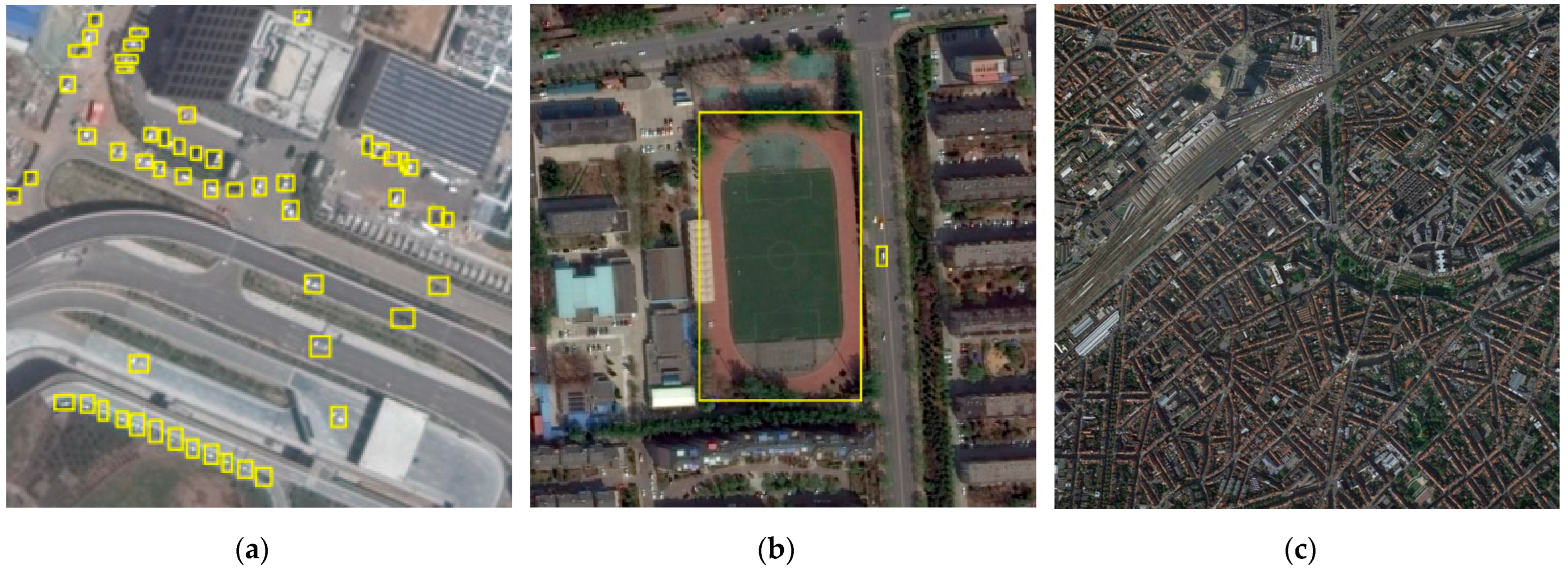
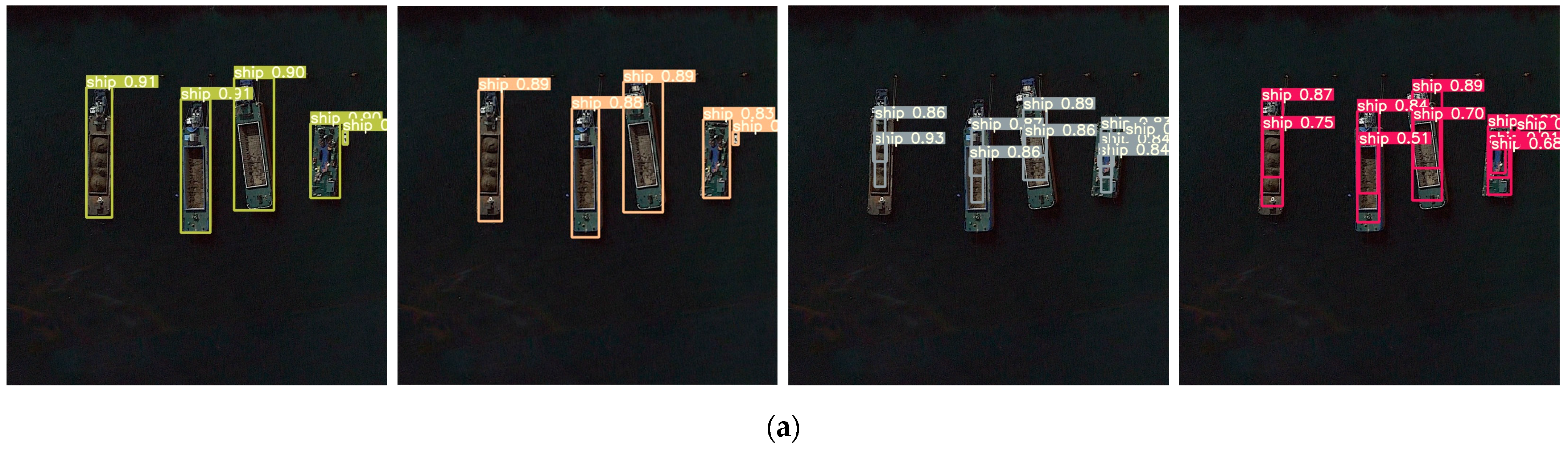
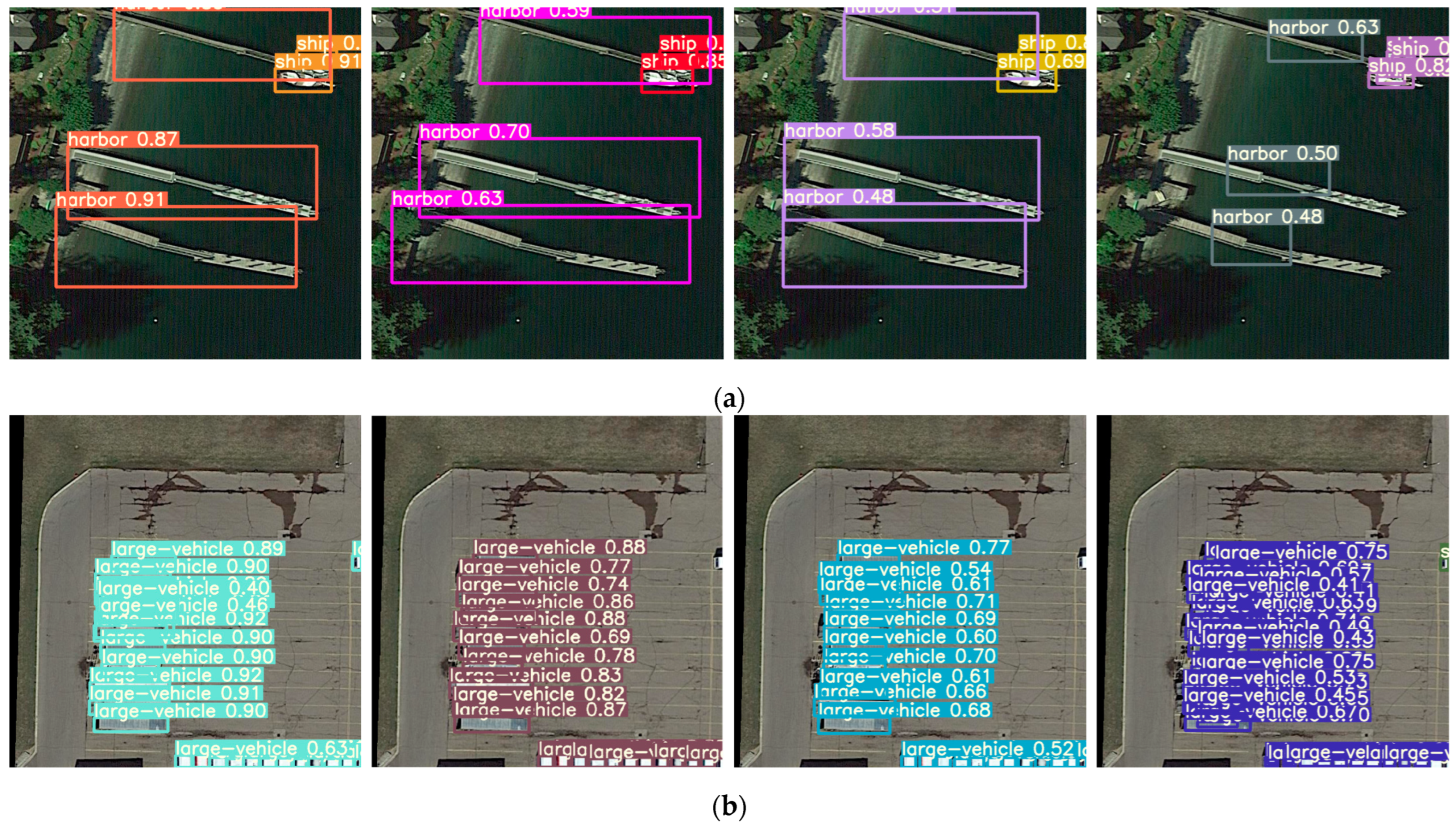
• The proportion of small objects is large. Small objects are easily missed due to a lack of feature information, which affects the detection effect. For example, there are more small targets in Figure 1a, which creates challenges in RSOD.
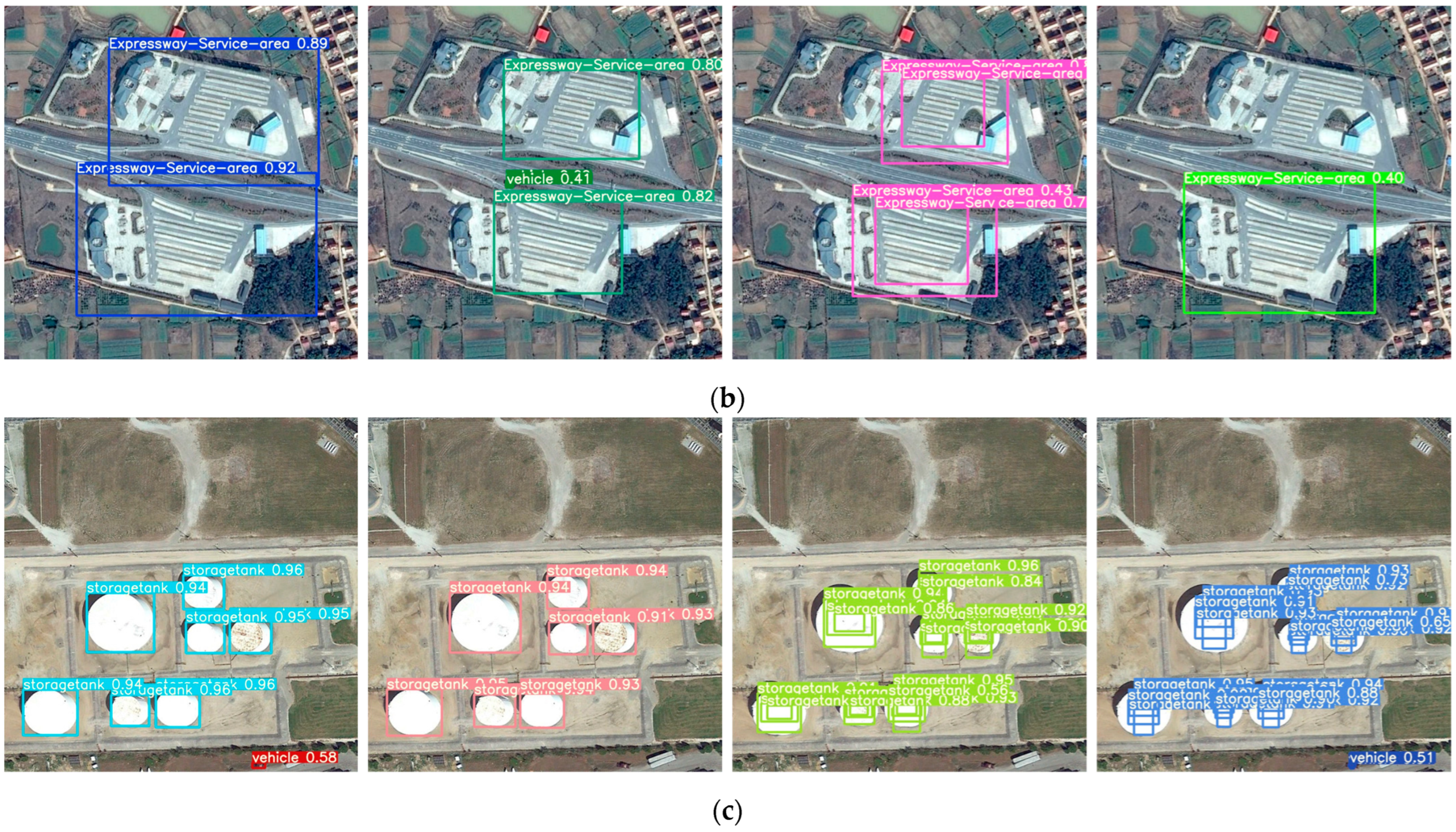
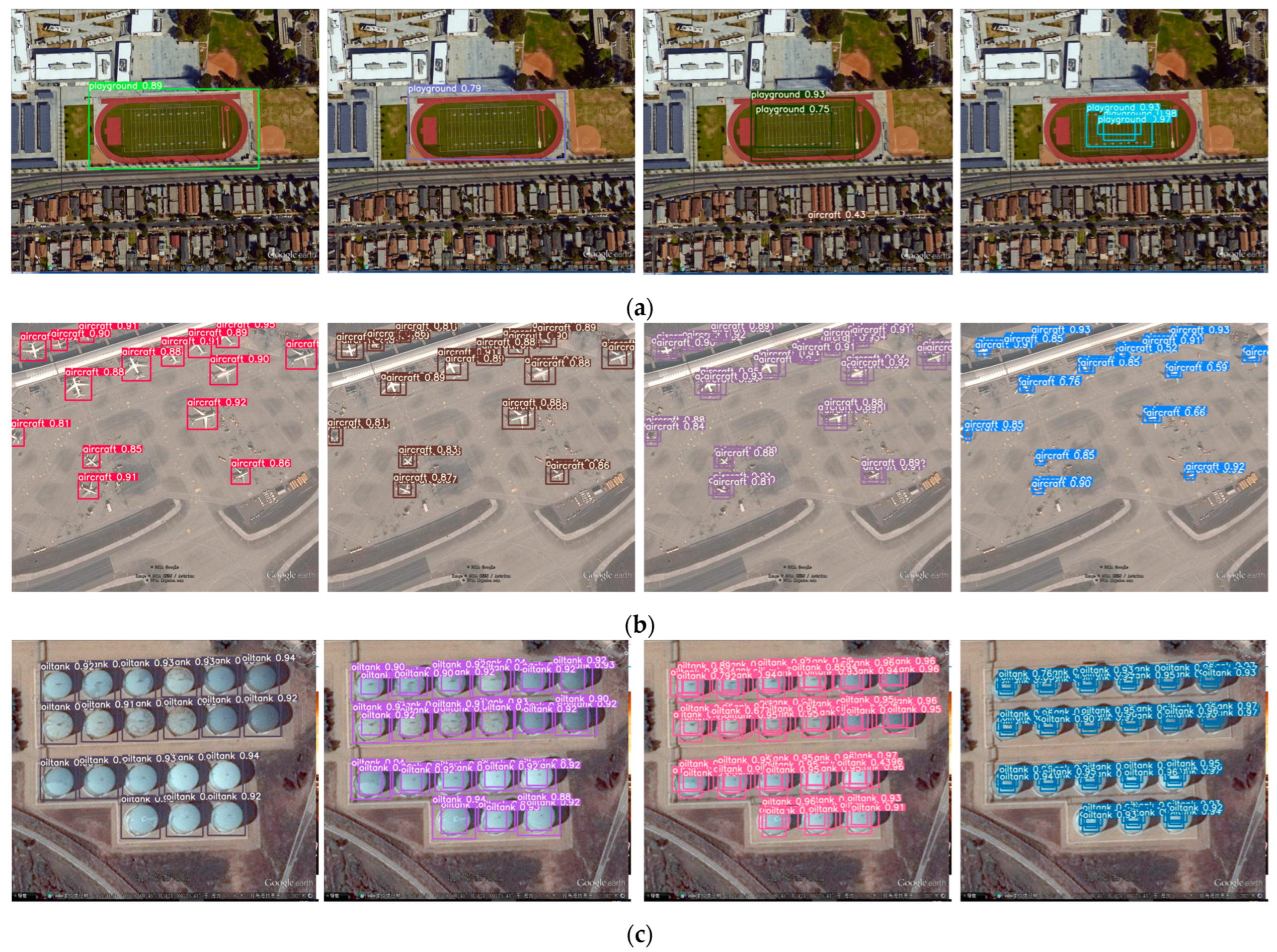
• The scales of objects greatly vary. Objects of the same category or different categories in RSIs are quite different in scale, and the scales presented by the same object may vary at different resolutions. As shown in Figure 1b, the scale of the playground is large, while that of the car is small, which requires the detection algorithm to have strong scale adaptability.
• The background is complex. As shown in Figure 1c, remote sensing imaging is influenced by light, weather, and terrain, which increases the background noise of RSIs and makes the objects hard to detect.

As traditional detection methods, the VJ Detector [3], the histogram of oriented gradients (HOG) [4], and the deformable parts model (DPM) [5] are mainly based on the manual extraction of features, and have high computational complexity. Deep learning-based methods can automatically extract features and have better performance. As two-stage methods, R-CNN [6], SPPNet [7], Fast R-CNN [8], and Faster R-CNN [9] have relatively high accuracy and low detection speed. One-stage algorithms, such as YOLO [10,11,12,13], improve the detection speed but are less accurate than two-stage algorithms. In recent years, one-stage algorithms have been migrated to the field of satellite observation and have obtained good detection performance. However, these methods are devised based on natural scene images. Compared to natural images, RSIs are obtained from remote distances, covering a wider range, and are influenced by factors such as lighting, weather, and terrain. Therefore, RSIs have more small objects, more multiscale objects, and more complex backgrounds. In this regard, some detection methods for RSIs have been proposed.

To enrich object features, Chen et al. [14] combined the shallowest features with semantic info and then enhanced and fused them with deep features. However, background noise was introduced. To reduce noise interference, Fu et al. [15] applied a balancing factor to balance the weight of feature fusion. However, this method is less robust to different tasks. Schilling et al. [16] used deconvolution to enlarge the scale of deep features and combined them with shallow features. Hou et al. [17] suggested a fusion tactic of cascade features, which fuses spatial features and semantic features to fuse the features of each layer and strengthen the cascade impression. Qu et al. [18] devised an efficient feature fusion network using extended convolution to enhance the effective perception field of deep features. Although the above methods ameliorate the problem of small targets in RSIs, they reduce the inference speed.

FPNs [19] fuse underlying visual characteristics with high-level semantic features and can predict on various scales. Yang et al. and Zou et al. [20,21,22] employed a dense feature pyramid based upon the FPN to additionally enhance the connection among characteristics of diverse scales. Fu et al. [23] increased an additional bottom-up connection after the top-down FPN to fuse the bottom features with the high-level visual features, which further enhanced feature expression ability. FMSSD [24] used the FPN and multiple sampling rates to form a spatial feature pyramid that fuses context information into multiscale features. These methods improve the performance of multiscale object detection. Nevertheless, the equilibrium between accuracy and velocity cannot be achieved well.

To reduce the background interference, Zhang et al. [25] extracted the feature mask of the objects and the background and introduced the pixel attention mechanism to weight the classes. However, this approach relies on prior knowledge and lacks universality. After extracting multiscale features, Li et al. [26] utilized the attention mechanism to enhance the features of each feature map. SCRDet [27] proposed a supervised attention network to decrease background noise. Li et al. [28] designed a salience pyramid fusion strategy to suppress background noise and introduced global attention mechanisms to enhance semantic information. Although attentional mechanisms can effectively weaken background information, they introduce additional mask calculations. Lightweight convolution is often used to reduce computational costs. Li et al. [29] proposed a lightweight convolutional called GSConv. Although this method requires more training data and increases tuning difficulty, the sparse connectivity and group convolution adopted lighten the model and maintain accuracy. Luo et al. [30] improved inference speed by improving the neck layer of YOLOv5 with GSConv.

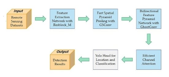
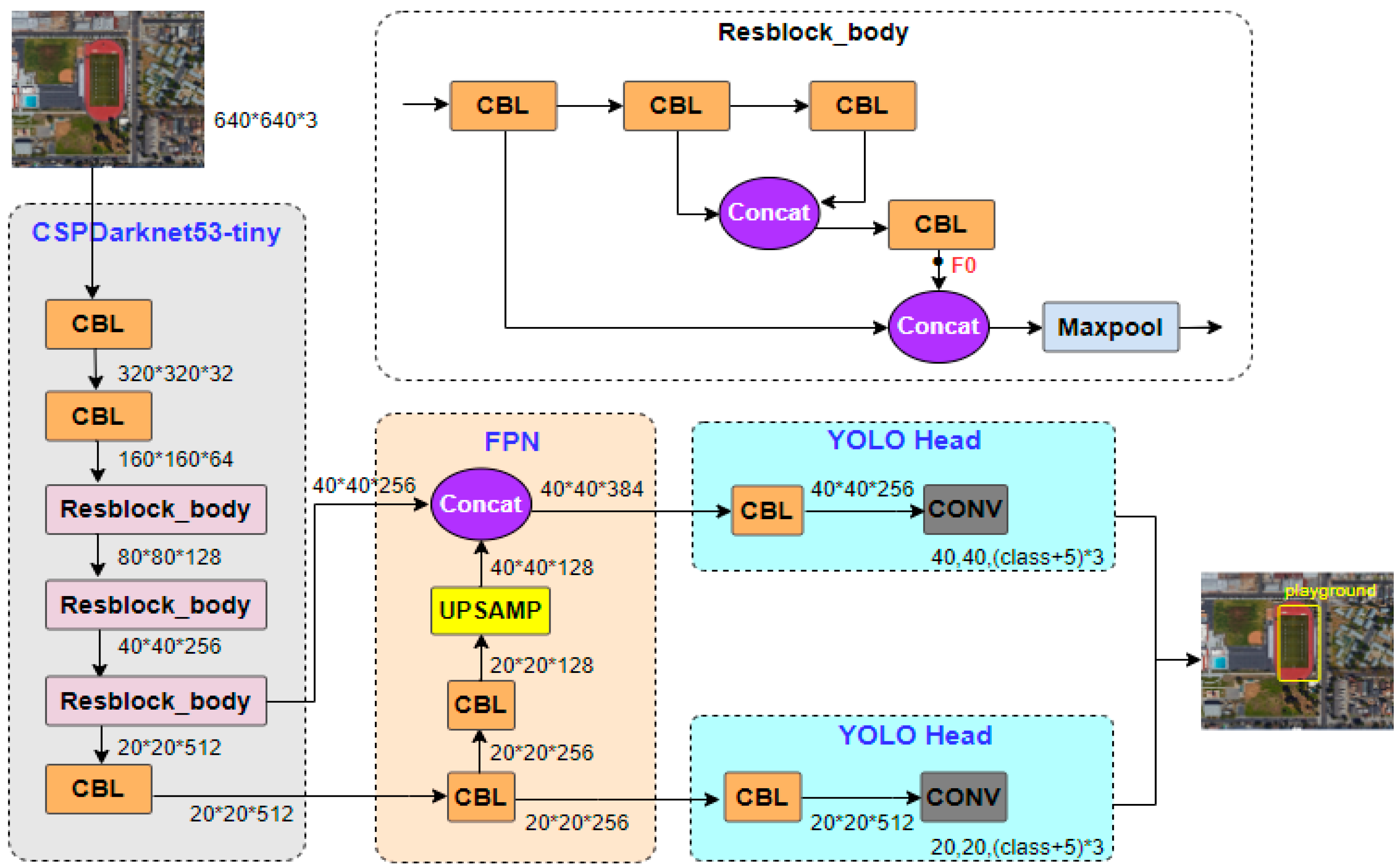
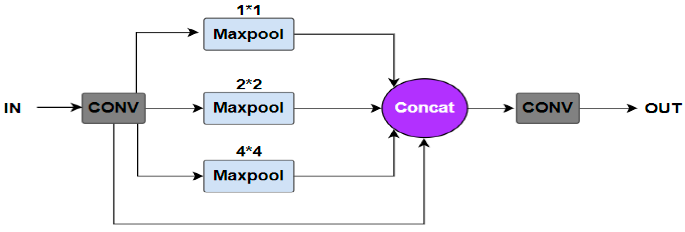
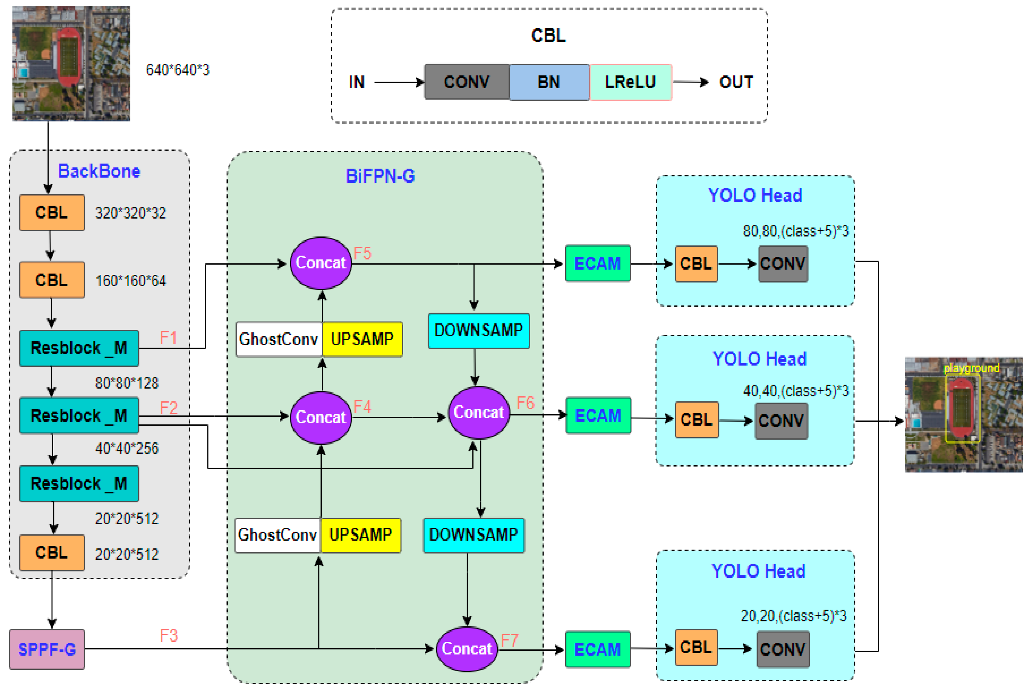
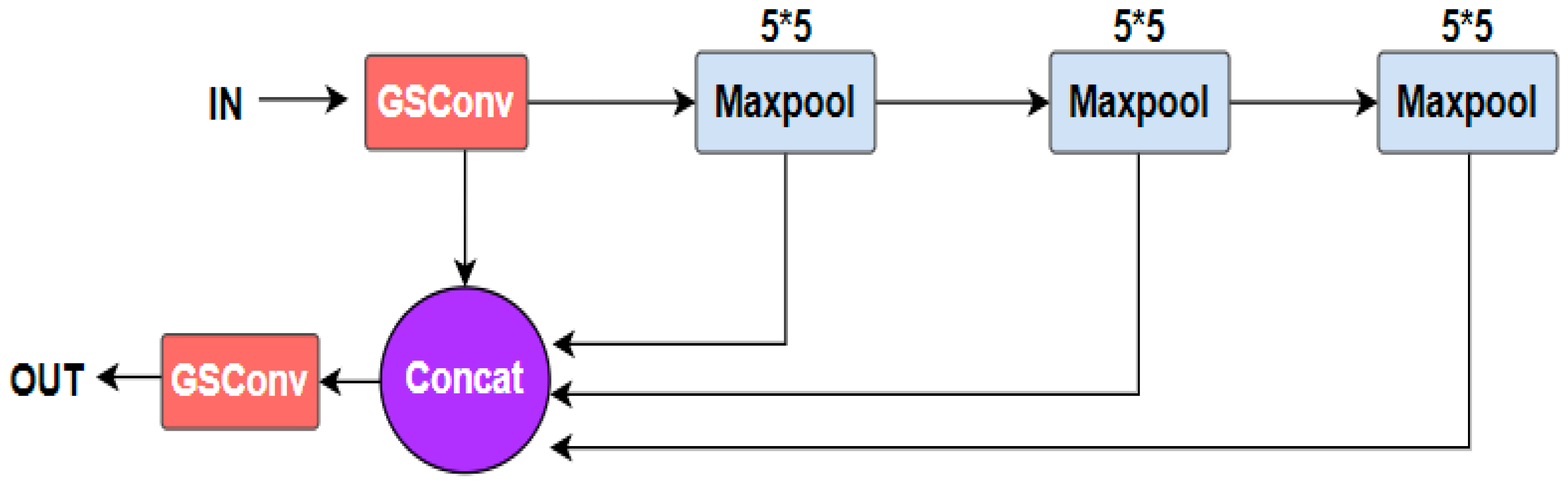
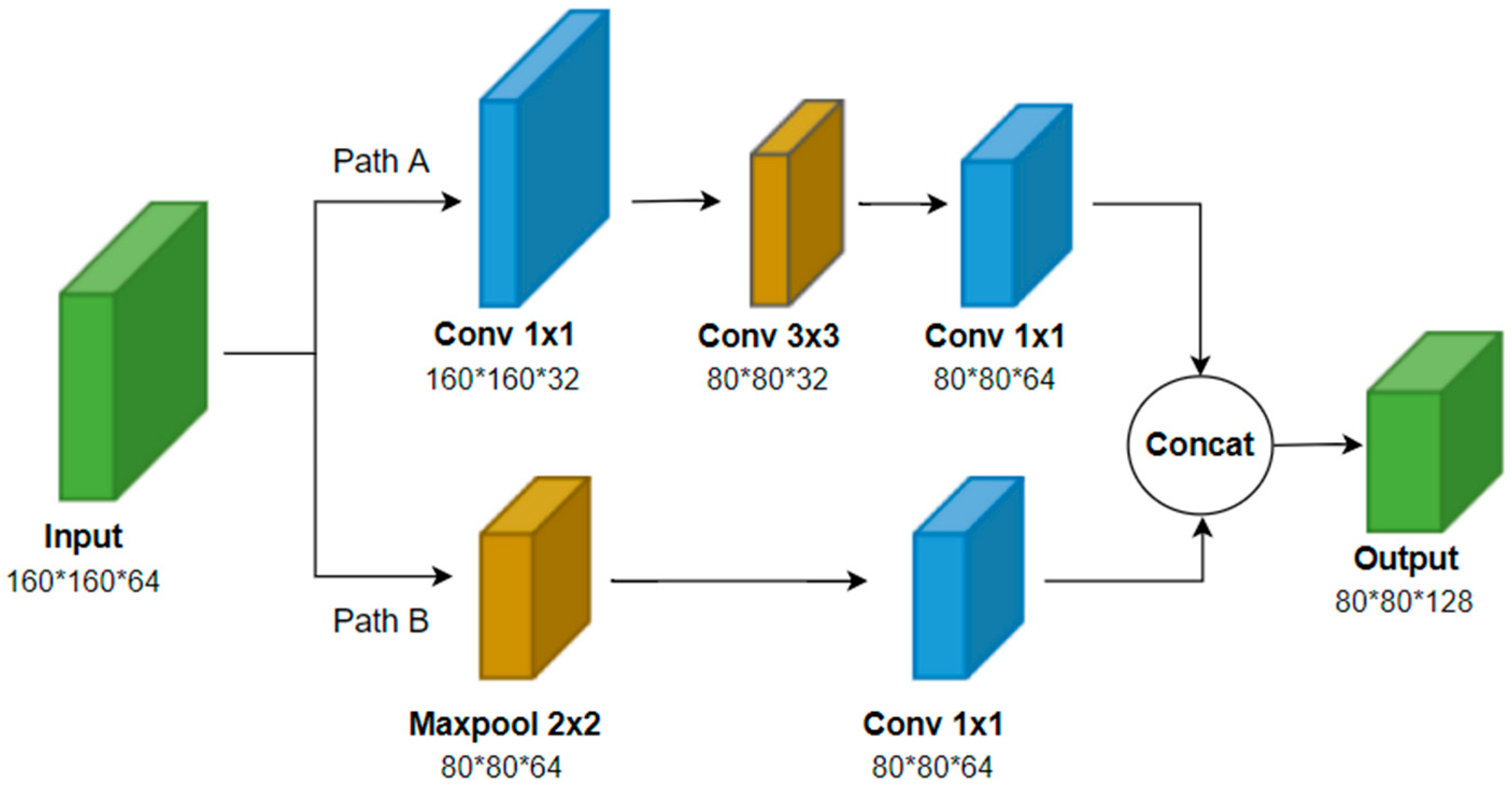
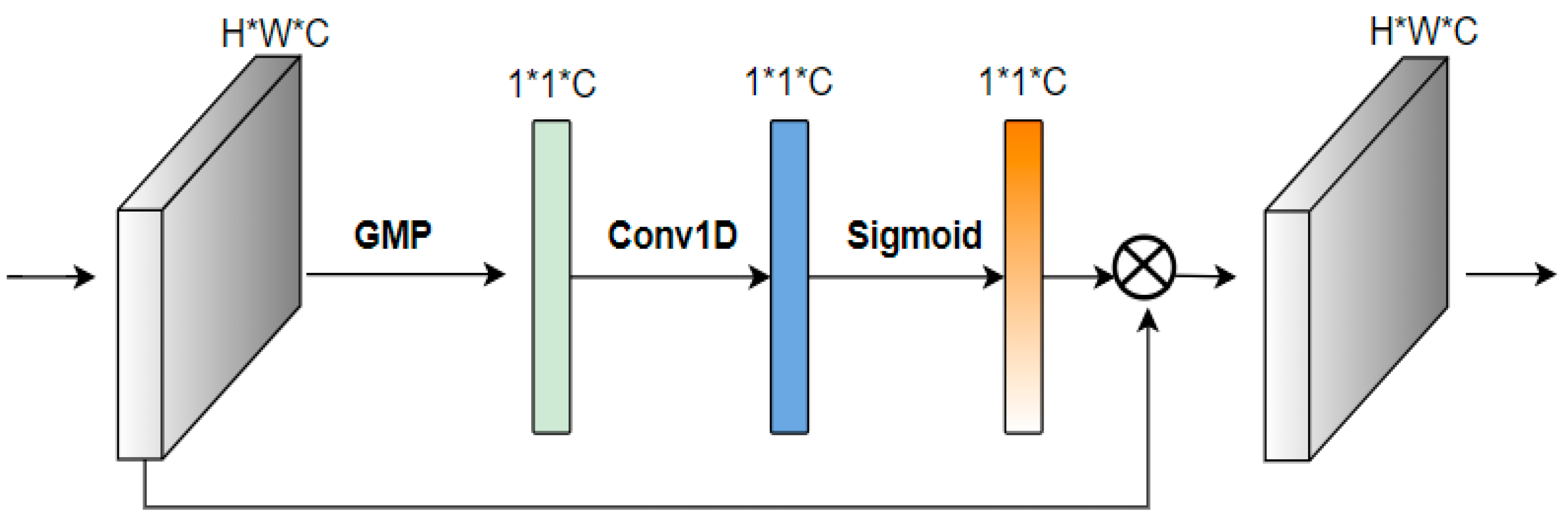
Inspired by the above methods, we propose a lightweight model that combines channel attention with multiscale feature fusion. First, we designed a fast spatial pyramid pooling incorporating GSConv (SPPF-G) for feature fusion [7], which fleshes out the spatial features of small targets. Second, the three-layer bidirectional feature pyramid network (BiFPN-G) [31] is suggested to integrate the deep semantic information with the shallow spatial information and to output the feature maps of different scales, which improves the scale adaptation ability of the model. Last, a novel efficient channel attention (ECAM) [32] is suggested to reduce background interference. The above methods reduce the inference speed; we constructed a new residual block (Resblock_M) [33] in the backbone to balance accuracy and speed.

The following are the contributions of this thesis:

• We designed SPPF-G for feature fusion, which fleshes out the spatial features of small targets and improves the detection accuracy of small objects.
• We modified the two-layer feature pyramid network (FPN) [19] to a three-layer BiFPN-G to integrate the deep semantic information with the shallow spatial information, thus improving the detection ability of the model for multiscale objects.
• We proposed the ECAM to enhance object information and suppress background noise and proposed a less computational residual block named Resblock_M to balance accuracy with speed.

The remainder of the paper is arranged as follows: Section 2 presents the relevant existing methods and our proposed method. Section 3 presents the experimental results obtained on different datasets. Section 4 is a discussion of the experimental results and future work. Section 5 is the summarization and future prospects of our work.

2. Methods

2.1. The Existing Methods

2.1.1. YOLOv4-Tiny

We used YOLOv4-tiny as the baseline. The model is faster than most algorithms and has few parameters, which is conducive to deployment on small devices with limited resources and is suitable for real-time RSOD. Figure 2 reveals the architecture of YOLOv4-tiny. The size of the input image is 640 × 640. As shown in Figure 2, the third residual block has two branches, one of which is nested with a residual block. The feature map with a size of 40 × 40 output by this branch is named $F_0$. The feature map with a size of 20 × 20 output from the last CBL in the backbone passes through two CBLs with a step size of 1 and upsampling, and the obtained feature map with a size of 40 × 40 is concatenated with $F_0$. YOLO Head is used for localization and classification, where the step size of both CBL and convolution is 1. If the step size is greater than 1, the input feature will be downsampled according to that step size during convolution, thereby reducing the size of the output feature map. If the step size is 1, the size of the feature map will not be changed.

2.1.2. Spatial Pyramid Pooling

The objects in RSIs are usually small and dense. Spatial pyramid pooling (SPP) [7] can realize feature fusion and solve the above problems. The architecture of SPP is revealed in Figure 3.

For an input image of any size, it first undergoes a convolution. Second, the feature map is grouped into 21 subblocks by the maximum pooling of 1 × 1, 2 × 2, and 4 × 4. Third, the maximum values are extracted from the 21 subblocks, thus transforming the input feature map of arbitrary size into a 21-dimensional feature of fixed size. Last, the 21-dimensional features are concatenated and convolved.

2.2. The Proposed Methods

2.2.1. Structure of BSFCDet

Figure 4 is the architecture of BSFCDet. BSFCDet proposes SPPF-G, the three-layer BiFPN-G, ECAM, and Resblock_M based on YOLOv4-tiny. The scale of the input image is 640 × 640. First, we input the picture and used the backbone to extract the feature map, where the designed residual block is less computed, which can improve the inference speed. Second, SPPF-G was employed to fuse the feature maps of various receptive fields after the backbone to enrich the expression power of the feature maps. Third, to boost the scale adaptation capacity, a three-layer BiFPN-G is suggested to integrate the spatial info of superficial layer feature maps and semantic info of in-depth feature maps and produce feature maps of separate measures. Fourth, the ECAM was built for the three scales of the feature map output of the BiFPN-G to further enrich the characteristics of the targets. Last, the feature regression prediction was made via the prediction output end. The decoding format is (class + 5) × 3, class represents the number of categories, 5 denotes the information about the anchor boxes: centre coordinates (x, y), width (w), height (h), and confidence, and 3 is the number of anchor boxes.

2.2.2. SPPF-G

However, the parallel pooling mode adopted by SPP requires processing multiple maximum pooling simultaneously, which increases computational time and memory usage. The pooling at different scales is carried out independently, which may extract similar features, leading to feature redundancy. As shown in Figure 5, to reduce feature redundancy, SPPF-G uses a serial structure, which involves sequentially performing maximum pooling; the results of each pooling are used as input for the next pooling, reducing the burden of processing multiple pooling simultaneously, thereby reducing computational time and memory consumption. Unifying the pooling kernels of different sizes of SPP into 5 × 5 makes features of different scales have same receptive fields for better feature fusion and detection. Larger pooling kernels can capture broader contextual information, more accurately represent the shape and structure of the objects, and require less computation, so SPPF-G uses the maximum pooling of size 5 × 5.

Traditional convolution uses dense connection, where each input channel is connected to each output channel. GSConv [29] uses sparse connectivity and group convolution, where input channels are grouped and each group is independently convolved, and each group is only connected to a portion of the output channels, which can reduce the computational complexity. GSConv uses the adaptive receptive field mechanism to dynamically adjust the size of the convolution kernel according to the spatial distribution of the input feature map, which enhances the diversity and expression ability of features, and the network’s adaptability to challenges such as complex scenes and small objects. So, SPPF-G uses GSConv instead of the traditional convolution.

As shown in

Table 1. Performance comparison between SPPF-G and SPP.

	GPU_mem (GB)	Forward (ms)	Backward (ms)	Input	Output
SPPF-G	4.401	54.84	114.3	(16,1024,64,64)	(16,1024,64,64)
SPP	4.586	80.9	171.2	(16,1024,64,64)	(16,1024,64,64)

, the forward and reverse calculation speed of SPPF-G is approximately 1.5 times higher than that of SPP. Experiments have shown that the calculation time of SPPF-G is shorter than that of SPP. After the backbone, we use more efficient SPPF-G to fuse the feature maps, which enlarges the receptive field of the picture, enriching the spatial features and detection effect of the small objects. Specifically, SPPF-G only reduces the calculation time of SPP rather than BSFCDet. Introducing SPPF-G into the model will still increase the computational complexity of the model, but it will increase less than SPP.

2.2.3. BiFPN-G

The objects’ scales vary greatly in RSIs. However, the FPN [19] is too simple, with only one upsampling and a single channel direction from top to bottom, and the output feature maps only have two scales, which easily lose the spatial info of superficial layer features and are not conducive to multiscale object detection. Therefore, we modified the FPN to a three-layer BiFPN-G, which outputs feature maps of three different scales.

In Figure 4, the feature map of the export of the first residual block in the backbone is named $F_1$ (80 × 80), the feature map of the export of the second residual block is named $F_2$ (40 × 40), and the feature map of the export of SPPF-G is named $F_3$(20 × 20). We carried out GhostConv [34] and upsampling of $F_3$ to enlarge the scale of the feature map to 40 × 40 and then concatenated it with $F_2$. The feature map after concatenation is named $F_4$ (40 × 40). A GhostConv and upsampling of $F_4$ are carried out to enlarge the scale of the feature map to 80 × 80 and then concatenate it with $F_1$. The feature map after concatenating is named $F_5$ (80 × 80). $F_5$ is subsampled once to change the scale of the feature graph to 40 × 40, and then it is concatenated with $F_2$ and $F_4$. The feature map after concatenation is named $F_6$ (40 × 40). $F_6$ is subsampled to change the scale of the feature graph to 20 × 20, and then it is concatenated with $F_3$. The feature map after concatenation is named $F_7$ (20 × 20). BiFPN-G outputs three different scale feature maps, $F_5$, $F_6$, and $F_7$, which advances detection accuracy for multi-scale objects.

Compared with the single-channel direction of the FPN from top to bottom, BiFPN-G adopts bidirectional transmission to combine the spatial info of superficial features and the semantic info of in-depth characteristics, which enhances the characterization ability of the backbone, avoids the loss of the spatial communication of superficial characteristics, and improves the fusion speed. This bidirectional structure can use not only the deep features transmitted by upsampling as the classification basis, but also the shallow spatial information transmitted by downsampling as the positioning basis. Small objects have only a small amount of info in the in-depth feature graph, so BiFPN-G adds a layer of output in the shallow layer to improve the recognition rate of small targets.

The number of convolution kernels of GhostConv is half that of the conventional convolution, which improves the inference speed of the model. GhostConv divides the channels of the input feature maps into main path and ghost path. The main path uses larger convolution kernels, while the ghost path uses smaller convolution kernels. This method of grouping feature channels can reduce the number of parameters. The ghost path repeatedly utilizes the feature maps in the main path for calculation, reducing computational complexity while enhancing the expression ability of the features.

2.2.4. ECAM

Influenced by light and other factors, the background info of RSIs is more complex. Furthermore, after multiple convolutions, the iterative accumulation of the background produces numerous redundant info, thus increasing the difficulty of detection. Many works sufficiently address these issues through attention mechanisms. The mechanism can not only preserve temporal location information but also obtain the differences among the feature maps in different channels and spatial dimensions and enhance the features of the objects. However, most attention modules have higher complexity. Compared with other attention mechanisms, the ECA [32] has higher efficiency while improving performance through the local cross-channel interaction strategy without dimensionality reduction.

However, the global average pooling (GAP) used by ECA is more suitable for large objects, while there are many small objects in the RSIs and the background is complex. The GAP will retain the background information, thus affecting the detection results. Therefore, GMP is applied to improve the ECA to obtain the ECAM, which requires less computation. We built three ECAMs after BiFPN-G to address the output feature maps of three scales, namely, $F_5$, $F_6$, and $F_7$. The structure of ECAM is shown in Figure 6.

First, GMP is performed on the input feature map to gain channel weights, and the scale of the resulting feature map is 1 × 1 × C. Second, to avoid dimension reduction, the local cross-channel interaction is realized with a 1D convolution with kernel size $k$, the dependence between channels is extracted, and the weight ($\omega$) of every channel is attained through the sigmoid activation function. The formula is presented as follows:

$$\omega =\sigma \left(C1D_k\left(y\right)\right)$$

(1)

where C1D represents 1D convolution, $\sigma$ represents the sigmoid activation function, and $y$ represents the feature map after GMP. The weights $\omega$ are multiplied channel-by-channel with the original input feature map to obtain features with channel attention. The ECAM not only weakens the background noise but also has minimal impact on the network processing speed due to the few parameters.

2.2.5. Resblock_M

Adding SPPF-G, BiFPN-G, and ECAM to the network can improve detection accuracy while increasing the number of layers and computational complexity of the network. Therefore, we replaced the residual blocks in the backbone with residual blocks with less computation, named Resblock_M, to balance accuracy and speed.

In Figure 7, Branch A performs a 1 × 1 convolution as well as a 3 × 3 convolution of the import feature map to halve the measurements of feature map, whereupon it performs a 1 × 1 convolution. Branch B performs a 2 × 2 maximum pooling on the input feature map to halve the measurements of feature map, whereupon it performs a 1 × 1 convolution. A feature map with half the size is obtained via concatenating the export feature maps of these two parts. Maximum pooling is utilized as it requires less computation than average pooling and does not retain background information. Compared to the residual block CSPBlock in YOLOv4-tiny, Resblock_M uses the 1 × 1 convolution of branch A instead of the 3 × 3 convolution in CSPBlock, reducing computation. Although Resblock_M adds two layers at branch B, the computation is still less than that of CSPBlock.

3. Results

3.1. Dataset and Preprocessing

Three datasets from the remote sensing fields, namely, DIOR [35], RSOD [36], and DOTAv1.0 [37], were selected. Moreover, to prove the universality of BSFCDet, non-remote sensing dataset PASCAL VOC2012 [38] was also selected.

Table 2. Specifics of the datasets.

Dataset	Categories	Images	Instances	Year	Proportion
DIOR	20	23,463	192,472	2018	1:1:2
RSOD	4	976	6950	2017	7:1:2
DOTAv1.0	15	20,889	188,282	2017	7:1:2
VOC12	20	17,125	40,138	2012	7:1:2

displays the details of each dataset. In addition to DIOR’s training set, verification data, and test data, which are stochastically grouped in a proportion of 1:1:2, the other three datasets are stochastically separated in a proportion of 7:1:2.

DIOR [35] is a large-scale dataset for object detection in optical RSIs, with 23,463 images and 192,472 instances, covering 20 types of objects. This dataset has the advantages of rich object scale and diverse images, which facilitates testing the performance of models in multiscale objects and complex backgrounds. RSOD [36] is an open dataset, including four object types: aircraft, playground, oil tank, and overpass. The dataset contains 976 images, covering 6950 objects. DOTAv1.0 [37] is an aerial image dataset annotated with horizontal boxes. Compared with other datasets, the data size of DOTA is larger, and the image resolution is higher. Since the aspect ratio of some pictures is too large to be directly utilized for training, we cut each picture into multiple 600 × 600 size pictures and generated corresponding annotation information for each cut picture. Then, we deleted the label files and corresponding pictures that did not meet the requirements, such as when an object is empty and out of bounds. The final dataset yielded a total of 20,889 images, 188,282 instances, and 15 object categories. VOC2012 [38] is a commonly employed object detection dataset with 20 object categories, 17,125 images, and 40,138 instances.

There is no fixed size ratio between small and large targets in RSIs. Some datasets have relatively larger size ratios, while others have relatively smaller size ratios, which can affect the setting of parameters of the proposed algorithm on each dataset. However, this impact is not significant. For example, to obtain optimal training results, appropriate training epochs and anchor boxes need to be set for each dataset. We used the static data analysis method k-means clustering to cluster the datasets before the training, obtaining a set of fixed-size anchor boxes as the initial prediction boxes, which is beneficial to accelerate the regression of the prediction boxes and increase the positioning precision.

Table 3. Anchor boxes used for the different datasets.

Dataset	Anchor
DIOR	(7,7)(8,16)(14,28)(19,11)(26,47)(36,20)(57,60)(107,128)(278,280)
RSOD	(14,15)(22,23)(30,29)(36,39)(47,48)(55,62)(68,74)(80,92)(223,275)
DOTAv1.0	(11,10)(20,22)(29,41)(43,25)(44,98)(47,45)(78,63)(100,106)(169,202)
VOC12	(21,40)(52,68)(62,141)(97,272)(159,155)(177,380)(303,495)(372,267)(549,556)

presents the anchor boxes used by BSFCDet on different datasets. Furthermore, to flesh out the image background, we used mosaic data augmentation as well as image flipping. The input pictures are randomly flipped, and then four images are selected for random cropping and spliced into an image as training data.

3.2. Experimental Setup and Comparative Methods

Our approach involves many parameters. The dimension of the entered picture during training is set to 640 × 640, and the batch size is 64. The dynamic learning rate method was adopted. The initial learning rate is 0.01, and the cosine annealing hyperparameter is 0.1. The momentum parameter of the gradient descent is 0.937. To prevent overfitting, the weight attenuation coefficient is 0.0005. During the training phase, the epochs for datasets DIOR, VOC12, RSOD, and DOTA are 300, 300, 1000, and 500.

Table 4. Experimental environment.

Parameter	Configuration
Operating System	Ubuntu 18.04
CPU	Intel Core i9-9900X CPU @3.50 GHz × 20
GPU	NVIDIA RTX 2080 Ti
Language	Python 3.8
Frame	PyTorch

unveils the experimental environment that we set up.

To validate the performance of BSFCDet, we compared BSFCDet with YOLOv4-tiny. In addition, in the comparative experiments, we also performed a comparison with classical and recent methods. In the DIOR dataset, we compared 22 methods, including R-CNN [6], Faster R-CNN [9], SSD [39], YOLOv5, YOLOv4 [13], YOLOv3-tiny [12], CSFF [40], and AFADet [41]. In the RSOD dataset, we compared 10 methods, including CenterNet [42], FANet [43], YOLOv3 [12], and YOLOv5s. For the datasets DOTA and VOC12, we compared the methods of YOLOv4, YOLOv3, and YOLOv3-tiny.

3.3. Evaluation Metrics

The IOU indicates the overlap of the prediction box and ground truth; the larger the IOU is, the more accurate the positioning. The object is generally detected when the IOU is not less than 0.5. The formula is presented as follows, where $A$ is the prediction box and $B$ is the ground truth:

$$IOU=\frac{A\cap B}{A\cup B}.$$

(2)

Precision is used to measure the probability of predicting true examples, and recall refers to the percentage of whole positives in test data that are aright recognized. The formulas are presented as follows:

$$Precision=\frac{TP}{TP+FP}.$$

(3)

$$Recall=\frac{TP}{TP+FN}.$$

(4)

where TP is the true-positive sample, FP is the false-positive sample, and FN is the false-negative sample. Precision and recall reflect two aspects of classifier performance; however, relying only on a single metric does not comprehensively evaluate the performance of a classifier. In order to consider precision and recall comprehensively, we introduced $F_1$ as a comprehensive indicator, inspired by Michael Buzzy et al. [44], which is the harmonic average of precision and recall. The formula is presented as follows:

$$F_1=\frac{2\times precision\times recall}{precision+recall}{.}_{}$$

(5)

Average precision (AP) is the specific value of the volume of aright identified objects to the sum of identified objects. A graph with precision as the ordinate and recall as the abscissa was constructed. The acreage encircled is AP. The mean of every class of AP is the mean average precision (mAP). The mAP at an IOU threshold of 0.5 is referred to as mAP@0.5. The IOU threshold ranges from 0.5 to 0.95, and the average mAP obtained with a step size of 0.05 is referred to as mAP@0.5:0.95. Frames per second (FPS) is the number of pictures recognized per second, which is a commonly employed indicator to assess the inference speed. Note that since the values of FPS are not unique per test, all of the values of FPS shown in this paper are the average values obtained after 50 experiments. The evaluation metrics utilized in this paper are mainly mAP@0.5, mAP@0.5:0.95, and FPS.

3.4. Ablation Experiment

To verify the importance of SPPF-G (S), BiFPN-G (B), ECAM (E), and Resblock_M (R), we performed an ablation experiment on the DIOR dataset, where the baseline is YOLOv4-tiny. The results are shown in

Table 5. Results of the ablation experiment.

	Baseline	+S	+S+B	+S+B+E	+S+B+E+R
Precision	42.5	49.8	50.5	51	44.6
Recall	61.4	66.2	69.7	71.4	68.4
F1	50.2	56.8	58.6	59.5	54
mAP@0.5	53	62.5	65.5	66.6	63.2
mAP@0.5:0.95	30.2	35.4	38	39.2	36.5
FPS	270	258	220	209	222

, where SPPF-G, BiFPN-G, and ECAM improve the recognition rate and Resblock_M improves the inference velocity.

From Table 5, it can be seen that the F1 score of YOLOv4-tiny is 50.2. SPPF-G increases F1 by 6.6, with the most significant improvement effect. BiFPN-G further increases F1 by 1.8, ECAM further increases F1 by 0.9, and Resblock_M sacrifices the F1 of 5.5 to improve detection speed. Compared with the baseline, BSFCDet’s F1 is 3.8 higher, with a significant improvement effect. Compared to the baseline, BSFCDet improves mAP@0.5 and mAP@0.5:0.95 by 10.2% and 6.3%, maintaining high real-time performance. Since the dataset that we chose mainly has problems with small objects, SPPF-G used to raise the recognition rate of tiny targets has the most significant effect. BiFPN-G enhanced mAP@0.5 and mAP@0.5:0.95 by 3% and 2.6%. Due to the simple ECAM structure and few computations, the increase in accuracy is not significant, but the lowest speed decreased compared to SPPF-G and BiFPN-G. These three modules also reduce the detection speed while improving accuracy, so the table shows that Resblock_M increases the FPS by 13 without much reduction in accuracy.

3.5. Comparative Experiments

YOLOv4, YOLOv3, YOLOv4-tiny, and YOLOv3-tiny are used as the comparison methods for all four datasets. Different comparison methods are also selected for different datasets. This is because different datasets have different representative algorithms, better-performing algorithms, and methods that have been widely studied and validated. Different datasets have different characteristics and challenges, some methods perform better on specific datasets while performing poorly on others; choosing more adaptable comparison methods can provide a more accurate and comprehensive performance comparison, thereby better demonstrating the improvement effects of our proposed method.

3.5.1. Comparative Experiments on DIOR

Table 6. Comparison of the detection speed of each algorithm.

Methods	Backbone	mAP@0.5	mAP@0.5:0.95	FPS	GPU	Year
Simple-CNN	VGG16	66.5	—	13	GT710	2021
CSFF	ResNet-101	68.0	—	15	RTX-3090	2021
CF2PN [47]	VGG16	67.3	—	20	RTX2080Ti	2021
AFADet	VGG16	66.1	—	26	RTX2080Ti	2022
YOLOv5l	—	71.2	45.8	28	GTX1070Ti	2020
ASSD-Lite [48]	MobileNetv2	63.3	—	35	GTX1080Ti	2021
YOLOv5m	Focus-CSP-SPP	69.8	44.6	46	GTX1070Ti	2020
AFADet-300	VGG16	57.4	—	61	RTX2080Ti	2022
YOLOv4	CSPDarkNet53	74.4	51.4	62	RTX2080Ti	2020
LO-Det	MobileNetv2	58.7	—	65	RTX3090	2021
YOLOv3	DarkNet53	57.1	49.9	89	RTX2080Ti	2018
YOLOv5s	CSP Focus	65.4	39.0	118	GTX1070Ti	2020
FANet	17-layer-CNN	56.5	—	228	RTX2080Ti	2021
YOLOv4-tiny	CSPDarkNet53tiny	53.0	30.2	270	RTX2080Ti	2020
YOLOv3-tiny	—	51.0	26.0	275	RTX2080Ti	2018
BSFCDet	CSPDarkNet53tiny-R	63.2	36.5	222	RTX2080Ti	2022

compares BSFCDet in terms of speed with other mainstream methods. According to the table, the FPS of BSFCDet is 222, which substantially exceeds Simple-CNN [45], CSFF [40], and other methods despite a slight decrease in accuracy, and the FPS of our algorithm is 209 higher than that of Simple-CNN [45]. Moreover, the accuracy and speed of BSFCDet surpass those of YOLOv3 [12], AFADet-300 [41], and LO-Det [46]. Although the accuracy of BSFCDet does not exceed that of the optimal YOLOv4 [13], the FPS of BSFCDet is 160 higher than the FPS of the optimal YOLOv4. Although FANet [43], YOLOv4-tiny [13], and YOLOv3-tiny [12] have a higher speed, BSFCDet has more advantages in relation to the detection effect. Otherwise, the other algorithms are slower than BSFCDet.

Table 7. Comparison of the detection accuracy of each algorithm.

	R-CNN	RICNN [49]	RICAOD [50]	YOLOv3-Tiny	YOLOv4-Tiny	Faster R-CNN
Backbone	VGG16	VGG16	VGG16	—	CSPDarkNet53tiny	VGG16
Airplane	35.6	39.1	42.2	73.3	58.7	53.6
Airport	43.0	61.0	69.7	25.5	56.1	49.3
Expressway toll station	33.5	36.6	49.3	50.2	48.7	55.2
Basketball court	62.3	66.3	79.0	82.5	74.4	66.2
Bridge	15.6	25.3	27.7	22.1	22.5	28.0
Chimney	53.7	63.3	68.9	71.7	72.0	70.9
Dam	33.7	41.1	50.1	22.7	47.5	62.3
Expressway service area	50.2	51.7	60.5	44.0	54.7	69.0
Baseball field	53.8	60.1	62.0	75.1	71.8	78.8
Golf course	50.1	55.9	64.4	28.5	60.4	68.0
Overpass	30.9	39.0	46.8	40.7	46.8	50.1
Harbor	39.5	43.5	42.3	34.8	51.3	50.2
Ground track field	49.3	58.9	65.3	56.5	64.5	56.9
Tennis court	54.0	63.5	70.3	81.8	79.8	75.2
Stadium	60.8	61.1	53.5	63.7	55.4	73.0
Storage tank	18.0	19.1	24.5	52.7	37.0	39.8
Ship	9.1	9.1	11.7	66.7	42.2	27.7
Train station	36.1	46.1	53.3	22.7	36.3	38.6
Vehicle	9.1	11.4	20.4	33.0	26.5	23.6
Windmill	16.4	31.5	56.2	72.4	52.6	45.4
mAP	37.7	44.2	50.9	51.0	53.0	54.1
	RIFD-CNN [51]	YOLOv3	SSD	Faster RCNN with FPN		BSFCDet
Backbone	VGG16	DarkNet53	VGG16	ResNet-50		CSPDarkNet53tiny-R
Airplane	56.6	72.2	59.5	54.1		79.0
Airport	53.2	29.2	72.7	71.4		62.7
Expressway toll station	56.0	54.4	53.1	62.1		57.4
Basketball court	69.0	78.6	75.7	81.0		86.0
Bridge	29.0	31.2	29.7	42.6		29.7
Chimney	71.5	69.7	65.8	72.5		74.0
Dam	63.1	26.9	56.6	57.5		39.9
Expressway service area	69.0	48.6	63.5	68.7		62.5
Baseball field	79.9	74.0	72.4	63.3		82.0
Golf course	68.9	31.1	65.3	73.1		65.4
Overpass	51.1	49.7	48.1	56.0		50.8
Harbor	51.2	44.9	49.4	42.8		50.2
Ground track field	62.4	61.1	68.6	76.5		66.6
Tennis court	79.5	87.3	76.3	81.2		85.5
Stadium	73.6	70.6	61.0	57.0		67.2
Storage tank	41.5	68.7	46.6	53.5		63.8
Ship	31.7	87.4	59.2	71.8		83.8
Train station	40.1	29.4	55.1	53.0		44.1
Vehicle	28.5	48.3	27.4	43.1		42.1
Windmill	46.9	78.7	65.7	80.9		71.7
mAP	56.1	57.1	58.6	63.1		63.2

(the red number is the highest value in each line, and the blue number is the second highest value in each line) compares the mAP@0.5 of each algorithm and AP values for 20 kinds of objects, which covers the classical algorithms, the most recent algorithms, and the algorithms for RSIs. It is not difficult to determine that BSFCDet achieves 63.2% mAP, outperforming other algorithms. Furthermore, BSFCDet has a 25.5% higher mAP than the classical R-CNN [6], a 10.2% higher mAP than YOLOv4-tiny [13], and a 12.2% higher mAP than YOLOv3-tiny [12].

Tennis courts, chimneys, basketball courts, and baseball fields are mainly shot from high altitudes, with complex backgrounds. Storage tanks and airplanes are also small and dense. However, the detection effect of BSFCDet ranks first on the airplane, basketball court, baseball field, and chimney, followed by expressway toll station, ship, storage tank, and tennis court. BSFCDet effectively improves the problems of RSOD, such as small objects and complex backgrounds.

To further prove the effectiveness of BSFCDet, we visualized the detection results. Figure 8 shows the representative detection examples of BSFCDet compared to other algorithms on the dataset DIOR. BSFCDet can more accurately locate complete objects and has higher accuracy. Compared to other algorithms, the proposed algorithm does not generate redundant boxes, and there is no omission or misdetection.

3.5.2. Comparative Experiments on RSOD

To verify the generalization of BSFCDet, we tested another dataset, RSOD. This dataset has many challenges, including small objects and complex backgrounds, which is beneficial to test the robustness of the network.

Table 8. Performance contrast of the different models on RSOD.

Methods	AI	OI	OV	PL	mAP@0.5	mAP@0.5:0.95	FPS
CenterNet	—	—	—	—	75.4	—	88
YOLOv3-tiny	90.7	92.2	61.3	88.9	83.3	51.2	276
SSD300	70.1	90.3	78.4	100	84.7	—	54
FANet	87.1	99.0	56.6	97.9	85.1	—	228
YOLOv4-tiny	90.9	91.8	68.0	90.0	85.2	53.7	274
Faster R-CNN	86.4	88.3	80.2	91.2	86.5	—	18
AFADet-300	69.8	96.9	93.4	99.9	90.0	—	61
YOLOv3	97.4	97.6	71.0	94.6	90.1	64.0	80
YOLOv5s	—	—	—	—	90.8	—	79
YOLOv4	98.4	98.5	76.3	98.4	92.9	65.7	60
BSFCDet	95.7	97.8	81.7	96.0	92.8	58.5	227

compares the performance of different models on RSOD where aircraft (AI), oil tank (OI), overpass (OV), and playground (PL) are the four types of objects. The red figure is the maximum in every column, and the blue figure shows the second largest value in every column.

Compared to YOLOv4-tiny, BSFCDet improves mAP@0.5 and mAP@0.5:0.95 by 7.6% and 4.8%, while maintaining a certain detection speed. Since the attention mechanism reduces background interference and the missing detection and misdetection rates, the detection effect of BSFCDet on the four types of objects has been greatly improved. The AP value of the overpass increases the most, which is the second largest value in all the results, only second to AFADet-300 [41]. Due to the lightweight design, BSFCDet is slightly inferior to YOLOv4 and YOLOv3 in terms of accuracy, but the FPS was improved by 167 and 147, respectively. The ECAM, SPPF-G, and BiFPN-G increase the computation amount of the network, and the detection speed of BSFCDet is not higher than that of YOLOv4-tiny and YOLOv3-tiny, but we obtained a more significant detection effect. The remaining algorithms, even the latest YOLOv5s, lag behind BSFCDet on precision and rate due to the lack of an attention mechanism and lightweight design. In conclusion, BSFCDet surpasses most algorithms, with strong generalization and robustness. In the face of the RSOD dataset with small objects and a complex background, BSFCDet achieves better performance and high real-time performance, effectively solves some challenges in the field of RSOD, and obtains the optimal balance between precision and pace.

Figure 9 shows the detection examples of BSFCDet compared to other algorithms on the dataset RSOD. BSFCDet has the best detection performance, especially when facing small and dense targets; BSFCDet still maintains better robustness.

3.5.3. Comparative Experiments on DOTA

Table 9. Performance contrast of the different models on DOTAv1.0.

Methods	mAP@0.5	mAP@0.5:0.95	FPS
YOLOv4	95.1	77.3	61
YOLOv3	93.2	75.6	86
YOLOv4-tiny	85.3	57.6	263
YOLOv3-tiny	84.3	52	280
BSFCDet	91.3	61.4	240

shows the performance contrast of the various algorithms on DOTAv1.0. DOTA has the advantages of rich object types and a large scale, which facilitates the training of the model. According to the table, BSFCDet increases the mAP@0.5 and mAP@0.5:0.95 of YOLOv4-tiny by 6% and 3.8%. Compared with YOLOv3-tiny, the mAP@0.5 and mAP@0.5:0.95 of BSFCDet are improved by 7% and 9.4%. Moreover, BSFCDet’s FPS exceeds YOLOv4’s and YOLOv3’s by 179 and 154, with a higher detection speed. Therefore, BSFCDet is undoubtedly optimal when considering precision and pace.

Figure 10 provides the detection examples of BSFCDet compared to other algorithms on the dataset DOTA. Most vehicles are small, and the distribution is relatively dense. However, SPPF-G reinforces the spatial info of tiny targets. Therefore, BSFCDet adequately locates these objects with high confidence. In addition, due to the multiscale fusion strategy, BSFCDet still achieves the best detection results in the face of harbors and ships with significant differences in size.

3.5.4. Comparative Experiments on VOC12

To enhance the universality of BSFCDet and demonstrate that BSFCDet is not only applicable to RSIs, we conducted experiments on a publicly available natural image dataset, VOC12.

Table 10. Performance comparison of the different models on VOC12.

Methods	mAP@0.5	mAP@0.5:0.95	FPS
YOLOv3-tiny	44	20.7	283
YOLOv4-tiny	46.5	23.3	284
R-CNN	53.3	—	50
YOLOv1	57.9	—	95
SPP-Net	58.1	—	51
YOLOv3	66	47	78
YOLOv4	68.3	49.1	71
BSFCDet	58.5	36.3	238

shows a performance comparison of the different models on VOC12. While maintaining high real-time performance, the mAP@0.5 and mAP@0.5:0.95 of BSFCDet are 12% and 13% higher than those of YOLOv4-tiny and 14.5% and 15.6% higher than those of YOLOv3-tiny, respectively. Compared to the classical R-CNN, YOLOv1, and SPP-Net, BSFCDet has more superiorities in both precision and speed. Compared with YOLOv3 and YOLOv4, we greatly improved the inference pace with only a mild reduction in precision. In conclusion, BSFCDet has strong universality, which not only achieves a good detection effect on remote sensing datasets but is also applicable to other datasets and has the most significant improvement effect on VOC12.

Figure 11 shows the detection examples of BSFCDet compared to other algorithms on the dataset VOC12. BSFCDet also has the best detection effect on non-RSIs.

4. Discussion

In this paper, we demonstrate that BSFCDet can maintain a better balance between detection accuracy and detection speed. The results may be attributed to the following facts. SPPF-G is used to achieve feature fusion, in which the serial pooling method reduces feature redundancy, and the size of maximum pooling is unified to 5 × 5, which increases the receptive field of the images and enriches the spatial information of small objects. GSConv improves the diversity of features and robustness of the network to small objects and complex backgrounds. The three-layer BiFPN-G integrates the semantic information of deep features and spatial information of shallow features, improving the detection ability of the model for multiscale objects. Adding an output layer in the shallow layer preserves more features of small objects, improving the recognition rate of small objects. ECAM reduces background interference and enhances object features. A residual block with smaller computational complexity balances the detection accuracy and speed of the model.

However, some limitations of this study still exist. Firstly, SPPF-G, BiFPN-G, and ECAM ignore the increase in parameter quantity, which reduces the detection speed, especially when the model introduces BiFPN-G with high computational complexity, resulting in a significant decrease in detection speed. Secondly, to balance accuracy and speed, Resblock_M loses some accuracy, but does not increase the speed too much. Finally, our method only considers small objects, multiscale objects, and complex backgrounds, without considering other issues such as object occlusion in RSIs.

In summary, in the future work, we will focus on accelerating the model by designing more lightweight networks to improve both the accuracy and inference speed of the model [52]. We will study the mixed use of non-maximum suppression (NMS) and Soft-NMS [53] in image post-processing, integrating the advantages of both, removing redundant bounding boxes, and improving the model’s robustness to object occlusion. Specifically, two thresholds, N1 and N2, are set. When IOU is higher than N1, traditional NMS is directly executed for filtering. When IOU is between N1 and N2, Soft-NMS is executed to reduce the confidence of overlapping anchor boxes. When IOU is lower than N2, no operation is performed.

5. Conclusions

In this paper, a lightweight RSOD method that combines channel attention and multiscale feature fusion is proposed. First, we propose SPPF-G to fuse the abstracted features and enrich the spatial info of small objects. Second, the two-layer single-channel structure of FPN [19] is modified to a three-layer BiFPN-G, which strengthens the detection capacity for multiscale targets. Third, by constructing the ECAM, the expressive ability of object features is enhanced. Last, Resblock_M, a lightweight residual block, is suggested to achieve a slight balance between accuracy and speed. We have performed tests on several datasets, and the data display that BSFCDet has strong generalization and robustness. In the future, we will research more lightweight models to attain improvements in both accuracy and speed, and improve the robustness of the model to object occlusion.

References

1. Wang, Y.; Bashir, S.M.A.; Khan, M.; Ullah, Q.; Wang, R.; Song, Y.; Guo, Z.; Niu, Y. Remote sensing image super-resolution and object detection: Benchmark and state of the art. Expert Syst. Appl. 2022, 197, 116793. [Google Scholar] [CrossRef]
2. Ma, W.; Li, N.; Zhu, H.; Jiao, L.; Tang, X.; Guo, Y.; Hou, B. Feature Split–Merge–Enhancement Network for Remote Sensing Object Detection. IEEE Trans. Geosci. Remote Sens. 2022, 60, 5616217. [Google Scholar] [CrossRef]
3. Viola, P.; Jones, M. Rapid object detection using a boosted cascade of simple features. In Proceedings of the 2001 IEEE Computer Society Conference on Computer Vision and Pattern Recognition, Kauai, HI, USA, 8–14 December 2001. [Google Scholar]
4. Dalal, N.; Triggs, B. Histograms of oriented gradients for human detection. In Proceedings of the 2005 IEEE Computer Society Conference on Computer Vision and Pattern Recognition (CVPR’05), San Diego, CA, USA, 20–25 June 2005; IEEE: San Diego, CA, USA, 2005; Volume 1, pp. 886–893. [Google Scholar]
5. Felzenszwalb, P.; McAllester, D.; Ramanan, D. A discriminatively trained, multiscale, deformable part model. In Proceedings of the IEEE Conference on Computer Vision & Pattern Recognition, Anchorage, AK, USA, 23–28 June 2008; pp. 1–8. [Google Scholar]
6. Girshick, R.; Donahue, J.; Darrell, T.; Malik, J. Rich Feature Hierarchies for Accurate Object Detection and Semantic Segmentation. In Proceedings of the IEEE Conference on Computer Vision and Pattern Recognition, Columbus, OH, USA, 23–28 June 2014; pp. 580–587. [Google Scholar] [CrossRef] [Green Version]
7. He, K.; Zhang, X.; Ren, S.; Sun, J. Spatial Pyramid Pooling in Deep Convolutional Networks for Visual Recognition. IEEE Trans. Pattern Anal. Mach. Intell. 2015, 37, 1904–1916. [Google Scholar] [CrossRef] [Green Version]
8. Girshick, R. Fast r-cnn. In Proceedings of the IEEE International Conference on Computer Vision, Santiago, Chile, 7–13 December 2015; pp. 1440–1448. [Google Scholar]
9. Ren, S.; He, K.; Girshick, R.; Sun, J. Faster R-CNN: Towards real-time object detection with region proposal networks. IEEE Trans. Pattern Anal. Mach. Intell. 2017, 39, 1137–1149. [Google Scholar] [CrossRef] [PubMed] [Green Version]
10. Redmon, J.; Divvala, S.; Girshick, R.; Farhadi, A. You only look once: Unified, real-time object detection. In Proceedings of the IEEE Conference on Computer Vision and Pattern Recognition, Las Vegas, NV, USA, 27–30 June 2016; pp. 779–788. [Google Scholar]
11. Redmon, J.; Farhadi, A. YOLO9000: Better, faster, stronger. In Proceedings of the IEEE Conference on Computer Vision and Pattern Recognition, Honolulu, HI, USA, 21–26 July 2017; pp. 7263–7271. [Google Scholar]
12. Redmon, J.; Farhadi, A. Yolov3: An incremental improvement. arXiv 2018, arXiv:1804.02767. [Google Scholar]
13. Bochkovskiy, A.; Wang, C.-Y.; Liao, M.H. YOLOv4: Optimal Speed and Accuracy of Object Detection. arXiv 2020, arXiv:2004.10934. [Google Scholar]
14. Chen, S.; Zhan, R.; Zhang, J. Geospatial Object Detection in Remote Sensing Imagery Based on Multiscale Single-Shot Detector with Activated Semantics. Remote Sens. 2018, 10, 820. [Google Scholar] [CrossRef] [Green Version]
15. Fu, Y.; Wu, F.; Zhao, J. Context-Aware and Depthwise-based Detection on Orbit for Remote Sensing Image. In Proceedings of the 2018 24th International Conference on Pattern Recognition (ICPR), Beijing, China, 20–24 August 2018. [Google Scholar]
16. Schilling, H.; Bulatov, D.; Niessner, R.; Middelmann, W.; Soergel, U. Detection of Vehicles in Multisensor Data via Multibranch Convolutional Neural Networks. IEEE J. Sel. Top. Appl. Earth Obs. Remote Sens. 2018, 11, 4299–4316. [Google Scholar] [CrossRef]
17. Hou, L.; Lu, K.; Xue, J.; Hao, L. Cascade detector with feature fusion for arbitrary-oriented objects in remote sensing images. In Proceedings of the 2020 IEEE International Conference on Multimedia and Expo (ICME), London, UK, 6–10 July 2020. [Google Scholar]
18. Qu, J.; Su, C.; Zhang, Z.; Razi, A. Dilated Convolution and Feature Fusion SSD Network for Small Object Detection in Remote Sensing Images. IEEE Access 2020, 8, 82832–82843. [Google Scholar] [CrossRef]
19. Lin, T.-Y.; Dollár, P.; Girshick, R.; He, K.; Hariharan, B.; Belongie, S. Feature pyramid networks for object detection. In Proceedings of the IEEE Conference on Computer Vision and Pattern Recognition (CVPR), Honolulu, HI, USA, 21–26 July 2017; pp. 2117–2125. [Google Scholar]
20. Yang, X.; Sun, H.; Sun, X.; Yan, M.; Guo, Z.; Fu, K. Position Detection and Direction Prediction for Arbitrary-Oriented Ships via Multitask Rotation Region Convolutional Neural Network. IEEE Access 2018, 6, 50839–50849. [Google Scholar] [CrossRef]
21. Yang, X.; Sun, H.; Fu, K.; Yang, J.; Sun, X.; Yan, M.; Guo, Z. Automatic Ship Detection in Remote Sensing Images from Google Earth of Complex Scenes Based on Multiscale Rotation Dense Feature Pyramid Networks. Remote Sens. 2018, 10, 132. [Google Scholar] [CrossRef] [Green Version]
22. Zou, F.; Xiao, W.; Ji, W.; He, K.; Yang, Z.; Song, J.; Zhou, H.; Li, K. Arbitrary-oriented object detection via dense feature fusion and attention model for remote sensing super-resolution image. Neural Comput. Appl. 2020, 32, 14549–14562. [Google Scholar] [CrossRef]
23. Fu, K.; Chang, Z.; Zhang, Y.; Xu, G.; Zhang, K.; Sun, X. Rotation-aware and multi-scale convolutional neural network for object detection in remote sensing images. ISPRS J. Photogramm. Remote Sens. 2020, 161, 294–308. [Google Scholar] [CrossRef]
24. Wang, P.; Sun, X.; Diao, W.; Fu, K. FMSSD: Feature-Merged Single-Shot Detection for Multiscale Objects in Large-Scale Remote Sensing Imagery. IEEE Trans. Geosci. Remote Sens. 2019, 58, 3377–3390. [Google Scholar] [CrossRef]
25. Zhang, Y.; You, Y.; Wang, R.; Liu, F.; Liu, J. Nearshore vessel detection based on Scene-mask R-CNN in remote sensing image. In Proceedings of the 2018 International Conference on Network Infrastructure and Digital Content (IC-NIDC), Guiyang, China, 22–24 August 2018; pp. 76–80. [Google Scholar]
26. Li, Q.; Mou, L.; Jiang, K.; Liu, Q.; Wang, Y.; Zhu, X.X. Hierarchical Region Based Convolution Neural Network for Multiscale Object Detection in Remote Sensing Images. In Proceedings of the IGARSS 2018–2018 IEEE International Geoscience and Remote Sensing Symposium, Valencia, Spain, 22–27 July 2018; pp. 4355–4358. [Google Scholar]
27. Yang, X.; Yang, J.; Yan, J.; Zhang, Y.; Zhang, T.; Guo, Z.; Sun, X.; Fu, K. SCRDet: Towards more robust detection for small, cluttered and rotated objects. In Proceedings of the IEEE International Conference on Computer Vision (ICCV), Seoul, Korea, 27 October–3 November 2019; pp. 8232–8241. [Google Scholar]
28. Li, C.; Luo, B.; Hong, H.; Su, X.; Wang, Y.; Liu, J.; Wang, C.; Zhang, J.; Wei, L. Object Detection Based on Global-Local Saliency Constraint in Aerial Images. Remote Sens. 2020, 12, 1435. [Google Scholar] [CrossRef]
29. Li, H.; Li, J.; Wei, H.; Liu, Z.; Zhan, Z.; Ren, Q. Slim-neck by GSConv: A better design paradigm of detector architectures for autonomous vehicles. arXiv 2022, arXiv:2206.02424. [Google Scholar]
30. Luo, W.; Zhang, Z.; Fu, P.; Wei, G.; Wang, D.; Li, X.; Shao, Q.; He, Y.; Wang, H.; Zhao, Z.; et al. Intelligent Grazing UAV Based on Airborne Depth Reasoning. Remote Sens. 2022, 14, 4188. [Google Scholar] [CrossRef]
31. Tan, M.; Pang, R.; Le, Q.V. Efficientdet: Scalable and efficient object detection. In Proceedings of the IEEE Conference on Computer Vision and Pattern Recognition (CVPR 2020), Washington, DC, USA, 14–19 June 2020; pp. 10781–10790. [Google Scholar]
32. Wang, Q.; Wu, B.; Zhu, P.; Li, P.; Zuo, W.; Hu, Q. Supplementary material for “ECA-Net: Efficient channel attention for deep convolutional neural networks”. In Proceedings of the 2020 IEEE/CVF Conference on Computer Vision and Pattern Recognition, IEEE, Seattle, WA, USA, 13–19 June 2020; pp. 11531–11539. [Google Scholar]
33. Jiang, Z.; Zhao, L.; Li, S.; Jia, Y. Real-time object detection method for embedded devices. In Proceedings of the Computer Vision and Pattern Recognition, Virtual, 14–19 June 2020. [Google Scholar]
34. Han, K.; Wang, Y.H.; Tian, Q.; Guo, J.Y.; Xu, C.J.; Xu, C. GhostNet: More Features from Cheap Operations. In Proceedings of the IEEE Conference on Computer Vision and Pattern Recognition (CVPR), Seattle, WA, USA, 14–19 June 2020; pp. 1577–1586. [Google Scholar]
35. Li, K.; Wan, G.; Cheng, G.; Meng, L.; Han, J. Object detection in optical remote sensing images: A survey and a new benchmark. ISPRS J. Photogramm. Remote Sens. 2020, 159, 296–307. [Google Scholar] [CrossRef]
36. Long, Y.; Gong, Y.; Xiao, Z.; Liu, Q. Accurate Object Localization in Remote Sensing Images Based on Convolutional Neural Networks. IEEE Trans. Geosci. Remote Sens. 2017, 55, 2486–2498. [Google Scholar] [CrossRef]
37. Xia, G.S.; Bai, X.; Ding, J.; Zhu, Z.; Belongie, S.; Luo, J.; Datcu, M.; Pelillo, M.; Zhang, L. DOTA: A Large-Scale Dataset for Object Detection in Aerial Images. In Proceedings of the 2018 IEEE/CVF Conference on Computer Vision and Pattern Recognition, Salt Lake City, UT, USA, 18–22 June 2018. [Google Scholar]
38. Everingham, M.; Eslami, S.M.A.; Van Gool, L.; Williams, C.K.I.; Winn, J.; Zisserman, A. The Pascal Visual Object Classes Challenge: A Retrospective. Int. J. Comput. Vis. 2014, 111, 98–136. [Google Scholar] [CrossRef]
39. Liu, W.; Anguelov, D.; Erhan, D.; Szegedy, C.; Reed, S.; Fu, C.; Berg, A.C. Ssd: Single shot multibox detector. In Proceedings of the European Conference on Computer Vision (ECCV), Amsterdam, The Netherlands, 8–16 October 2016; pp. 21–37. [Google Scholar]
40. Cheng, G.; Si, Y.; Hong, H.; Yao, X.; Guo, L. Cross-Scale Feature Fusion for Object Detection in Optical Remote Sensing Images. IEEE Geosci. Remote Sens. Lett. 2020, 18, 431–435. [Google Scholar] [CrossRef]
41. Wang, J.; Gong, Z.; Liu, X.; Guo, H.; Yu, D.; Ding, L. Object Detection Based on Adaptive Feature-Aware Method in Optical Remote Sensing Images. Remote Sens. 2022, 14, 3616. [Google Scholar] [CrossRef]
42. Duan, K.; Bai, S.; Xie, L.; Qi, H.; Huang, Q.; Tian, Q. CenterNet: Keypoint triplets for object detection. In Proceedings of the IEEE International Conference on Computer Vision (ICCV), Seoul, Korea, 27 October–3 November 2019; pp. 6568–6577. [Google Scholar]
43. Lang, L.; Xu, K.; Zhang, Q.; Wang, D. Fast and Accurate Object Detection in Remote Sensing Images Based on Lightweight Deep Neural Network. Sensors 2021, 21, 5460. [Google Scholar] [CrossRef] [PubMed]
44. Buzzy, M.; Thesma, V.; Davoodi, M.; Velni, J.M. Real-Time Plant Leaf Counting Using Deep Object Detection Networks. Sensors 2020, 20, 6896. [Google Scholar] [CrossRef] [PubMed]
45. Arriaga, O.; Valdenegro-Toro, M.; Plöger, P. Real-time Convolutional Neural Networks for Emotion and Gender Classification. arXiv 2017, arXiv:1710.07557. [Google Scholar]
46. Huang, Z.; Li, W.; Xia, X.-G.; Wang, H.; Jie, F.; Tao, R. LO-Det: Lightweight Oriented Object Detection in Remote Sensing Images. IEEE Trans. Geosci. Remote. Sens. 2021, 60, 3067470. [Google Scholar] [CrossRef]
47. Wei, H.; Zhang, Y.; Chang, Z.; Li, H.; Wang, H.; Sun, X. Oriented objects as pairs of middle lines. ISPRS J. Photogramm. Remote Sens. 2020, 169, 268–279. [Google Scholar] [CrossRef]
48. Xu, T.; Sun, X.; Diao, W.; Zhao, L.; Fu, K.; Wang, H. ASSD: Feature Aligned Single-Shot Detection for Multiscale Objects in Aerial Imagery. IEEE Trans. Geosci. Remote Sens. 2021, 60, 3089170. [Google Scholar] [CrossRef]
49. Cheng, G.; Zhou, P.; Han, J. Learning Rotation-Invariant Convolutional Neural Networks for Object Detection in VHR Optical Remote Sensing Images. IEEE Trans. Geosci. Remote Sens. 2016, 54, 7405–7415. [Google Scholar] [CrossRef]
50. Li, K.; Cheng, G.; Bu, S.; You, X. Rotation-Insensitive and Context-Augmented Object Detection in Remote Sensing Images. IEEE Trans. Geosci. Remote Sens. 2017, 56, 2337–2348. [Google Scholar] [CrossRef]
51. Cheng, G.; Zhou, P.; Han, J. Rifd-cnn: Rotation-invariant and fisher discriminative convolutional neural networks for object detection. In Proceedings of the IEEE Conference on Computer Vision and Pattern Recognition (CVPR), Las Vegas, NV, USA, 26 June–1 July 2016; pp. 2884–2893. [Google Scholar]
52. Zou, Z.; Chen, K.; Shi, Z.; Guo, Y.; Ye, J. Object Detection in 20 Years: A Survey. arXiv 2019, arXiv:1905.05055. [Google Scholar] [CrossRef]
53. Bodla, N.; Singh, B.; Chellappa, R.; Davis, L.S. Soft-nms—Improving object detection with one line of code. In Proceedings of the IEEE International Conference on Computer Vision (ICCV) 2017, Venice, Italy, 22–29 October 2017; pp. 2380–7504. [Google Scholar]
Figure 1. Challenges of RSOD. The object to be detected is surrounded by the yellow box. RSIs where the objects are (a) small, (b) multiscale, and (c) difficult to distinguish from the background.
Remotesensing 15 03213 g001
Figure 2. Structure of YOLOv4-tiny.
Remotesensing 15 03213 g002
Figure 3. Structure of SPP.
Remotesensing 15 03213 g003
Figure 4. Structure of BSFCDet.
Remotesensing 15 03213 g004
Figure 5. Structure of SPPF-G.
Remotesensing 15 03213 g005
Figure 6. Structure diagram of the ECAM.
Remotesensing 15 03213 g006
Figure 7. Structure diagram of Resblock_M.
Remotesensing 15 03213 g007
Figure 8. Detection examples of BSFCDet compared to other algorithms on the dataset DIOR. (a) Comparison of detection examples for image 1; (b) Comparison of detection examples for image 2; (c) Comparison of detection examples for image 3. The algorithms corresponding to each row from left to right are BSFCDet, YOLOv3, YOLOv4-tiny, and YOLOv3-tiny.
Remotesensing 15 03213 g008aRemotesensing 15 03213 g008b
Figure 9. Detection examples of BSFCDet compared to other algorithms on the dataset RSOD. (a) Comparison of detection examples for image 1; (b) Comparison of detection examples for image 2; (c) Comparison of detection examples for image 3. The algorithms corresponding to each row from left to right are BSFCDet, YOLOv3, YOLOv4-tiny, and YOLOv3-tiny.
Remotesensing 15 03213 g009
Figure 10. Detection examples of BSFCDet compared to other algorithms on the dataset DOTA. (a) Comparison of detection examples for image 1; (b) Comparison of detection examples for image 2; (c) Comparison of detection examples for image 3. The algorithms corresponding to each row from left to right are BSFCDet, YOLOv3, YOLOv4-tiny, and YOLOv3-tiny.
Remotesensing 15 03213 g010aRemotesensing 15 03213 g010b
Figure 11. Detection examples of BSFCDet compared to other algorithms on the dataset VOC12. (a) Comparison of detection examples for image 1; (b) Comparison of detection examples for image 2; (c) Comparison of detection examples for image 3. The algorithms corresponding to each row from left to right are BSFCDet, YOLOv3, YOLOv4-tiny, and YOLOv3-tiny.
Remotesensing 15 03213 g011