Article

Application of a New Hybrid Deep Learning Model That Considers Temporal and Feature Dependencies in Rainfall–Runoff Simulation

School of Geography and Planning, Sun Yat-sen University, Guangzhou 510275, China
*
Author to whom correspondence should be addressed.
Remote Sens. 2023, 15(5), 1395; https://doi.org/10.3390/rs15051395
Submission received: 7 January 2023 / Revised: 23 February 2023 / Accepted: 28 February 2023 / Published: 1 March 2023

Abstract

:
Runoff forecasting is important for water resource management. Although deep learning models have substantially improved the accuracy of runoff prediction, the temporal and feature dependencies between rainfall–runoff time series elements have not been effectively exploited. In this work, we propose a new hybrid deep learning model to predict hourly streamflow: SA-CNN-LSTM (self-attention, convolutional neural network, and long short-term memory network). The advantages of CNN and LSTM in terms of data extraction from time series data are combined with the self-attention mechanism. By considering interdependences of the rainfall–runoff sequence between timesteps and between features, the prediction performance of the model is enhanced. We explored the performance of the model in the Mazhou Basin, China; we compared its performance with the performances of LSTM, CNN, ANN (artificial neural network), RF (random forest), SA-LSTM, and SA-CNN. Our analysis demonstrated that SA-CNN-LSTM demonstrated robust prediction with different flood magnitudes and different lead times; it was particularly effective within lead times of 1–5 h. Additionally, the performance of the self-attention mechanism with LSTM and CNN alone, respectively, was improved at some lead times; however, the overall performance was unstable. In contrast, the hybrid model integrating CNN, LSTM, and the self-attention mechanism exhibited better model performance and robustness. Overall, this study considers the importance of temporal and feature dependencies in hourly runoff prediction, then proposes a hybrid deep learning model to improve the performances of conventional models in runoff prediction.

Graphical Abstract

1. Introduction

Floods are among the most common natural disasters, and extreme precipitation is often the main cause of flood disasters. Thus, the rainfall–runoff model is important for studies of basin hydrological processes with the goal of preventing flood disasters [1,2,3]. However, runoff prediction is highly complex, dynamic, and unstable; thus, it remains challenging for hydrologists to achieve efficient and accurate runoff prediction [4,5,6]. Models for runoff prediction can be divided into two categories: physical process-based and data-driven [7,8].
Physical process-based models are mathematical models that systematically describe the hydrological processes of a basin. They can be subdivided into lumped and distributed types. Lumped models generalize and assume the hydrological processes of a basin. Such models perform calculations for the entire basin but they do not consider spatial heterogeneity with respect to climate and underlying surface factors. Examples of lumped models include HEC-HMS [9,10], HBV [11], and XAJ [12]. Distributed models solve the problem of homogenization of watershed physical characteristics that exists in lumped models. The watershed is divided into fine meshes for calculations of runoff generation and concentration that can fully reflect the watershed physical characteristics and rainfall spatial distribution. Examples of distributed models include SWAT [13,14], SHE [15,16], and Liuxihe [17,18,19]. Although distributed hydrological models have been applied to watershed hydrological forecasting, they have some limitations. These models attempt to simulate physical mechanisms of the hydrological process, thus improving interpretability; however, the increase in model complexity creates a need for additional input data and physical parameters, which leads to poor model portability and an increasing need for high-precision physical property data [20]. Additionally, some processes of the hydrological cycle cannot be accurately described, leading to necessary simplifications in the hydrological model calculation process and the inevitable introduction of simulation error [21,22].
Compared with process-based hydrological models, data-driven models are completely based on internal relationships between the data fitting input and the output; because such models lack a clear understanding of the internal physical mechanisms, they avoid generalization of the hydrological runoff generation and concentration processes [23,24,25]. These models have been widely used for runoff prediction. In early research regarding data-driven hydrological models, ARMA and its improved models were often used to predict runoff time series [26,27]. However, because these models are linear, they have considerable limitations in complex hydrological applications. Nonetheless, advances in machine learning allowed some nonlinear models to become popular. In 1986, Rumelhart proposed a backpropagation algorithm to train the network, which solved the problem of artificial neural network (ANN) parameter training [28]. Thus, ANN models have been widely used in hydrological forecasting [29,30]. However, ANNs have problems such as overfitting, gradient disappearance, and sequence information loss; accordingly, these simple models are inappropriate for complex hydrological processes [31]. With the exponential growth of sample data and improvements in computing power, complex deep learning models (e.g., convolutional neural network [CNN] and long short-term memory network [LSTM]) have demonstrated strong capabilities and robust performance in the field of hydrology. Because of their excellent feature extraction abilities, CNNs can extract repetitive patterns hidden in hydrology time series [32,33]. Recurrent neural networks (RNNs) transform hidden nodes into a cyclic structure, serialize the input data when learning nonlinear relationships between input and output, and adequately capture temporal dynamics [34]. However, RNNs are susceptible to problems of gradient disappearance or gradient explosion during backpropagation. A variant of the RNN approach, LSTM models use a gate mechanism and introduce memory cells to store long-term memory, thereby solving the RNN bottleneck involving long-term dependence; accordingly, LSTMs have been studied in the field of hydrology [35,36,37]. Kratzert et al. tested the effect of LSTM in ungauged watersheds using K-fold cross-validation in the CAMELS dataset. The experiment showed that the data-driven model had better performance than the traditional physical model under out-of-sample conditions [38]. Mao et al. proved the importance of hydrological hysteresis to LSTM runoff simulation by experiments [39].
In recent years, with the continuous development of research on rainfall–runoff data-driven models, some ensemble models or hybrid models began to appear. Francesco et al. proposed a novel simpler model based on the stacking of the Random Forest and Multilayer Perceptron algorithms, which performed similar to the excellent performance of the bidirectional LSTM, but had the notable advantage of much shorter computation times than the bidirectional LSTM [40]. Kao et al. proposed a Long Short-Term Memory based Encoder-Decoder (LSTM-ED), and compared it with a feed forward neural network-based Encoder-Decoder (FFNN-ED) model to prove the superiority of the model for multi-step-ahead flood forecasting [41]. Cui et al. developed a data-driven model by integrating singular spectrum analysis (SSA) and a light gradient boosting machine (LightGBM) to achieve the high-accuracy, real-time prediction of regional urban runoff [42]. Yin et al. proposed a novel data-driven model named LSTM-based multi-state-vector sequence-to-sequence (LSTM-MSV-S2S) rainfall–runoff model, which contained m multiple state vectors for m-step-ahead runoff predictions, and compared it with two LSTM-S2S models by testing them on CAMELS data set. The results showed that LSTM-MSV-S2S model has better performance [43]. Chang et al. proposed a novel urban flood forecast methodology framework by integrating the advantages of Principal Component Analysis (PCA), Self-Organizing Map (SOM), and Nonlinear Autoregressive with Exogenous Inputs (NARX) to mine the spatial–temporal features between rainfall patterns and inundation maps for making multi-step-ahead regional flood inundation forecasts [44].
Although the new proposed hybrid rainfall–runoff models constantly has greatly improved the accuracy of runoff prediction, previous research regarding data-driven models has not effectively used temporal and feature dependencies between rainfall–runoff time series elements. Temporal dependencies reflect the importance of variation in time series data according to time frequency. Additionally, rainfall station observations, an important input feature, often indicate that rainfall frequency is closer when the distance is smaller. To improve model accuracy, temporal and feature dependencies should be exploited, rather than ignored [45,46,47].
In this study, we consider temporal and feature dependencies. CNN and LSTM models are used to extract the characteristics of rainfall–runoff, and explore the temporal and feature dependencies of rainfall–runoff input with the self-attention mechanism. We propose a new hybrid streamflow prediction model, namely SA-CNN-LSTM, that considers interdependences between timesteps and features of the rainfall–runoff series; this model can improve the performance of hourly predicted runoff.

2. Methodologies

2.1. Self-Attention Mechanism

The attention mechanism is currently widely used in various deep learning tasks, such as natural language processing, image recognition, and speech recognition [48,49,50]. In accordance with the selective attention aspect of human vision, it considers extensive available information, then selects information that is more relevant to the current task goal by assigning different weights [51]. In this study, the self-attention mechanism was used in the output matrix of LSTM and CNN to extract interdependences between timesteps and features. The attention mechanism can be regarded as the contribution of source to target, which represents the mapping of a query vector to a series of key-value pair vectors [52]. The process can be divided into three steps: (1) calculation of similarity between query and key vectors to obtain target weight; (2) normalization of weight; and (3) multiplication of the value vector by the weight vector to assign weight. The special case in which the source equals the target constitutes the self-attention mechanism.
Suppose that an output vector h R m × k of LSTM is selected as the input of the self-attention mechanism. In the expression, m represents the number of features in a single timestep, and k represents the number of timesteps.
h m × k = h m 1 , h m 2 , h m i , , h m k
The attention weight α of each hidden layer output vector is computed by
S i = F ( W q h m i , W k h m i )
α i = S o f t m a x S i = exp S i j = 1 k exp S j
V = W v h m 1 α 1 , W v h m 2 α 2 , W v h m i α i , , W v h m k α k
where W q ,   W k , and W v are the query, key, and value weight matrix, respectively (all obtained by training); F is usually a scaled dot product; α i is the weight of timestep I; and V represents the result of assigning weight to each timestep.

2.2. Neural Network

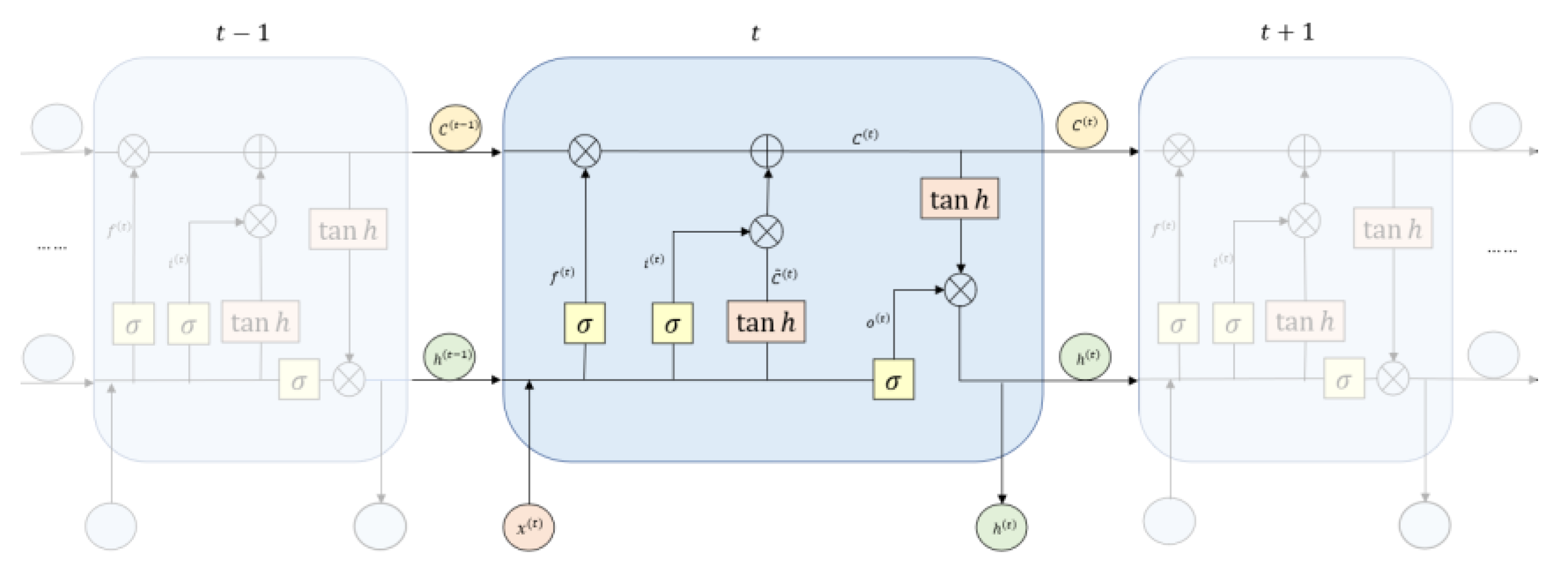
2.2.1. Long Short-Term Memory Network

LSTM models are RNN variants that add or delete time series memory information by adjusting gate states [53]. The LSTM unit calculation process contains three inputs: the memory cell state C t 1   and   hidden   state   ( h t 1 ) , passed down from the previous timestep, respectively, which represent long-term memory and short-term memory, as well as the current timestep,   X t . According to   X t and h t 1 , there are four internal states, z i ,   z f ,     z o , and   z , which are estimated as follows:
z = t a n h w x t + w h t 1 + b
z i = S i g m o i d w i x t + w i h t 1 + b i
z f = S i g m o i d w f x t + w f h t 1 + b f
z o = S i g m o i d w o x t + w o h t 1 + b o
In Equations (5)–(8), w and b represent the weight and the deviation, respectively; tanh and sigmoid represent the activation function; and z i ,   z f ,   z o ,   and z represent the input gate, forget gate, output gate, and input information, respectively. Figure 1 shows the internal structure of the LSTM, which mainly progresses through three stages:
Forget stage: z f , as the forget gate signal, controls the C t 1 passed down from the last timestep to perform selective forgetting.
Memory stage: z i , as the input gate signal, selectively remembers from the current timestep x t .
Output stage: z o , as the output gate signal, selectively outputs from the updated memory cell state   C t to obtain the hidden state   h t at the current timestep.
The mathematical expressions of processes in the three stages are as follows:
C t = z f C t 1 + z i z  
h t = z O tanh C t  
y t = s i g m o i d w t h t
where   C t and   h t   represent the updated memory cell state and updated hidden state in the current timestep, respectively; y t   is an output of the current timestep. ⊙ represents matrix multiplication.

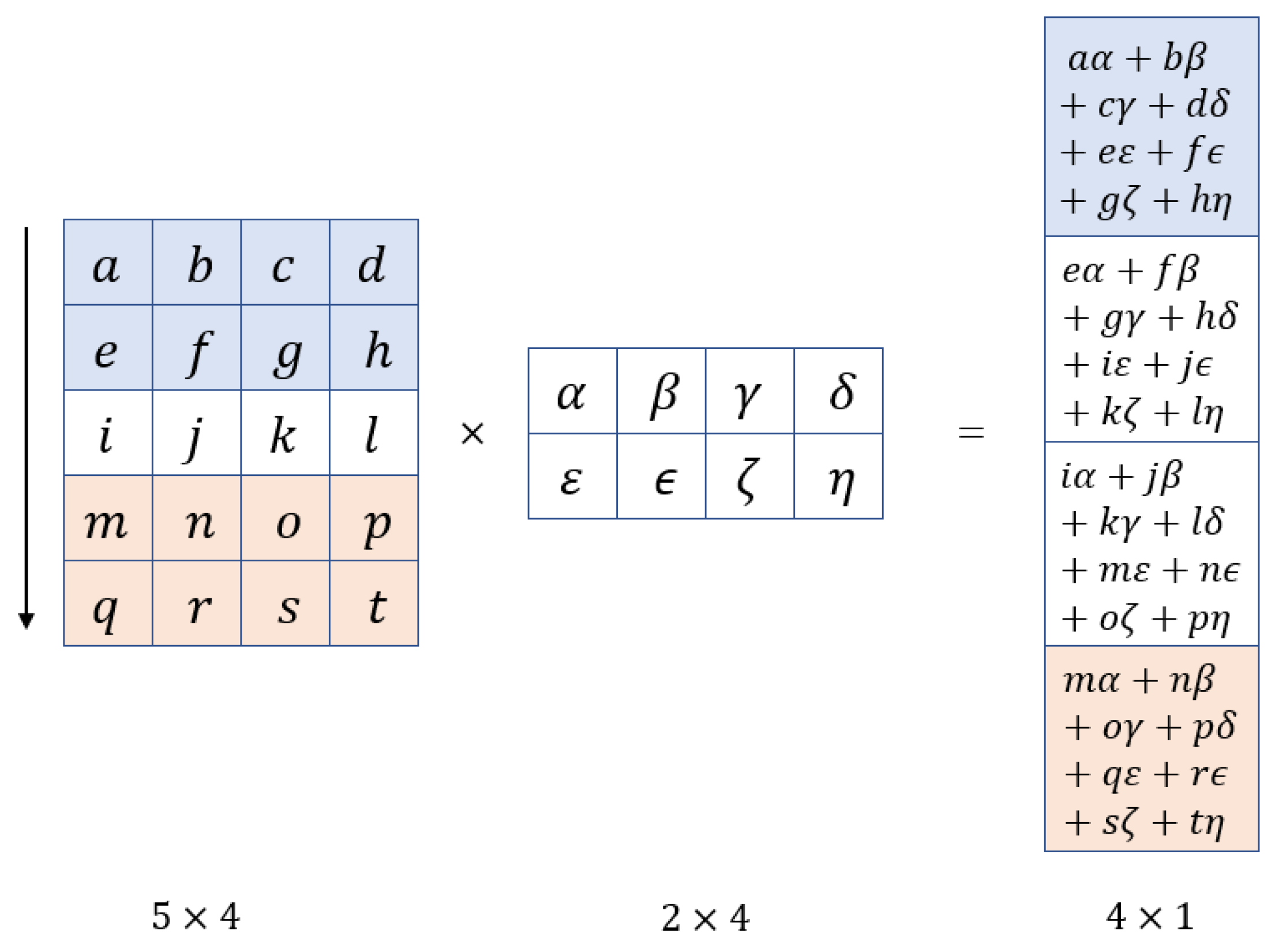
2.2.2. Convolutional Neural Network

CNNs are deep neural network models based on the cognitive mechanism of natural biological vision; they are particularly successful in image recognition [54] and object detection [55]. Sparse connection and parameter sharing are the most prominent features of CNNs, which have excellent feature extraction capabilities that distinguish them from conventional ANN models [56]. CNNs extract features through convolution operations, which usually scan entire datasets according to input order, as well as preset convolution core size, convolution stride size, and padding size. At each step of scanning, the convolution kernel and the input data of corresponding rows and columns are used for matrix multiplication and matrix addition. CNN-based time series prediction methods all use one-dimensional convolution operations to study the trend of the time series itself. The one-dimensional convolution operation process focused on time series data is shown in Figure 2.

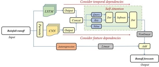
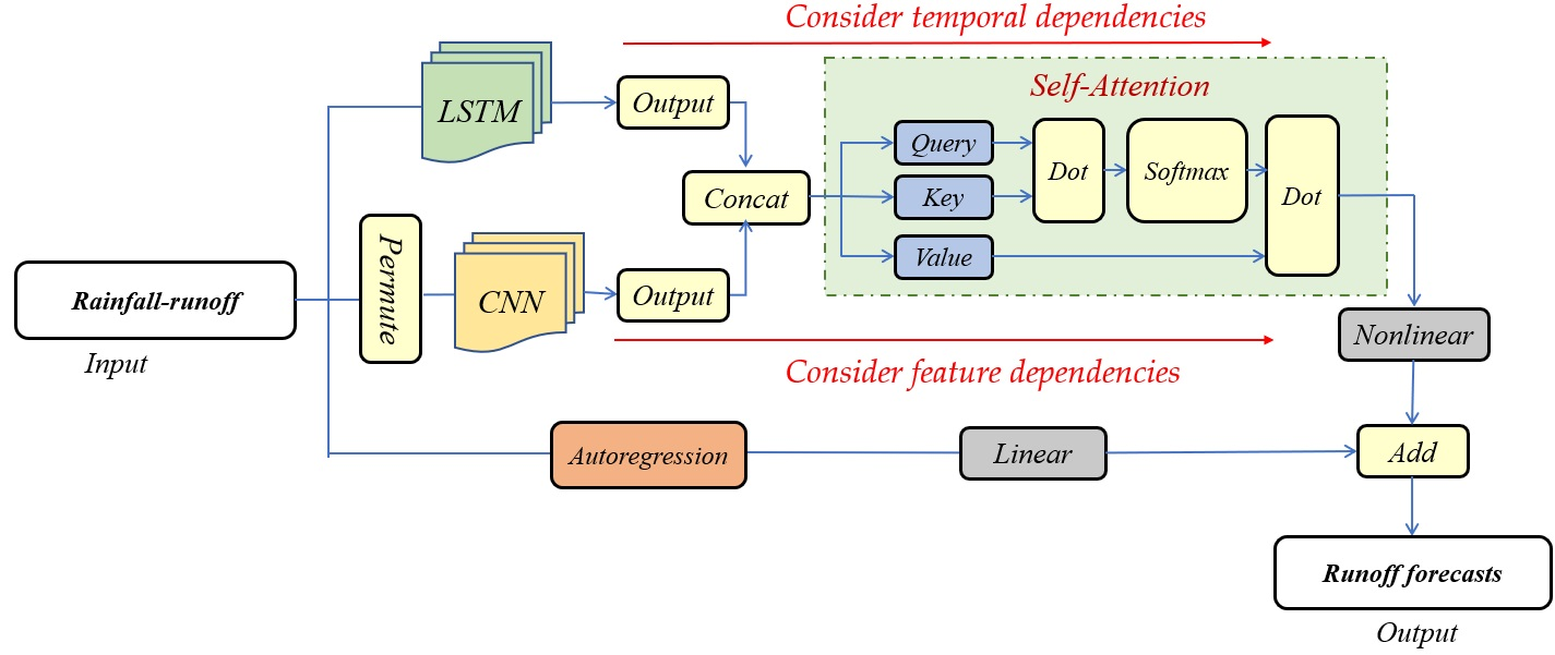
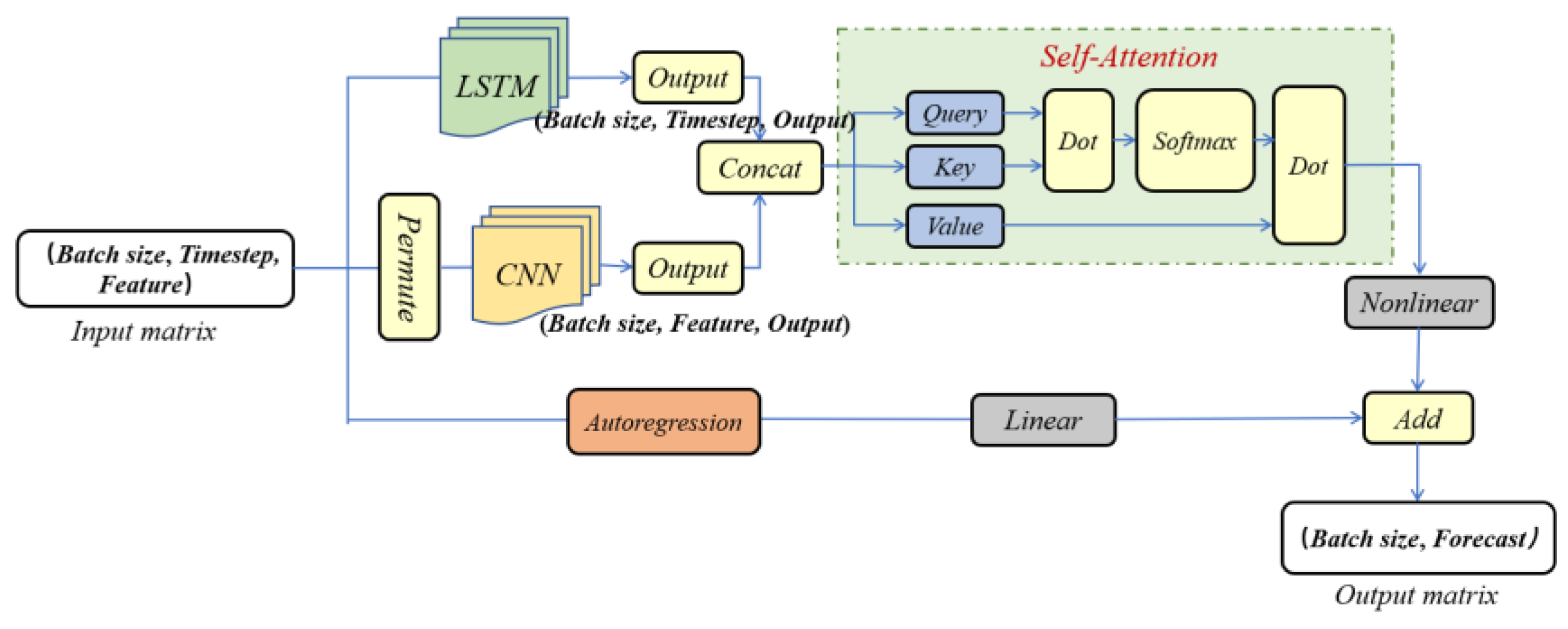
2.3. SA-CNN-LSTM Model

The SA-CNN-LSTM model integrates the excellent abilities of CNNs and LSTMs to extract feature patterns. The self-attention mechanism is used to learn temporal and feature dependencies from the output feature matrix, then assign weights. The model mainly progresses through two stages of processing from data input to output. In the first stage, the input matrix is sent to the LSTM to obtain information regarding each timestep; the transposed input matrix (timestep dimension and feature dimension transposition) is sent to the CNN for a one-dimensional convolution operation that yields information regarding each input feature. The self-attention mechanism is used to assign weights to features extracted by the two models. This mechanism assigns weights to the output matrices of the two models in their respective timesteps and feature dimensions. In the second stage, in addition to the above nonlinear relationship, the model adds an autoregressive layer to consider the linear relationship with respect to runoff [57,58]. Finally, the output results of the two stages are summed and input into the feedforward neural network to yield the final prediction results. A flowchart of the SA-CNN-LSTM is shown in Figure 3. In the Figure, the input matrix is a batch of data samples. A single input sample is I n p u t 1 = X 1 , X 2 , , X t , , X T , Q 1 , where X and Q represent meteorological and hydrological stations data, respectively, and T is the timestep. X = X 1 , X 2 , X 3 , , X T is the historical rainfall sequence of T timestep, and Q = Q 1 , Q 2 , Q 3 , , Q T is the historical runoff sequence of T timestep. The output matrix is a batch of prediction results. A single output sample is O u t p u t 1 = Y 1 , Y 2 , , Y m , where Y m represents the result of predicted runoff in the next m hours.

2.4. Network Structure Optimization

The time of confluence at the outlet point is closely related to the physical characteristics of the basin. To determine the timestep of the input model, the Pearson correlation coefficient is used to calculate the correlation between rainfall and runoff. The calculation formula is as follows:
R δ = i N F i + δ F ¯ R i R ¯ i N F i + δ F ¯ 2 i N R i R ¯ 2
where F , F ¯ , R , and R ¯ represent runoff, average runoff, precipitation, and average precipitation, respectively; δ represents the offset between runoff and rainfall time. The correlation coefficient curves of different offsets are shown in Figure 4. The impact of hourly rainfall on change in runoff first increases and then decreases; it eventually reaches the same magnitude as the starting point after 60 h, indicating that hourly rainfall can effectively influence the change in runoff in the basin over the next 60 h.
Based on the results of the correlation coefficient curve calculated above, we set the timestep to 60 h for prediction of runoff at the outlet of the basin in the next 7 h. The Adam optimizer was chosen as the model optimization algorithm [59,60], and mean square error was regarded as the loss function. Other super-parameters of the model (e.g., LSTM hidden layer dimension, CNN layer dimension, autoregression layer dimension, attention layer dimension, and learning rate) need to be set in advance before training. The parameter optimization of the deep learning model has always been a very complex problem. In this experiment, we choose to use the Hyperopt library provided by python to help optimize the super-parameters, where fmin() is the function to call the parameter optimization. This function mainly contains four parameters. The first parameter is to set the target function as MSE, the second parameter is to set the parameter optimization range, as shown in Table 1, the third parameter is to set the number of iterations as 1000, and the fourth parameter is to set the parameter optimization method as random search method.

2.5. Evaluation Statistics

In this study, the Nash efficiency coefficient (NSE), root mean square error (RMSE), mean absolute error (MAE), mean relative error (MRE), and peak error (PE) were used to evaluate the performance of the proposed model.
N S E = 1 i = 1 N O i P i 2 i = 1 N O i O ¯ 2
R M S E = 1 N i = 1 N O i P i 2
M A E = i = 1 N O i P i N
M R E = 1 N i = 1 N ( O i P i O i
P E = O f P f O f
where O i ,   O ¯ , P i , O f and   P f represent the runoff observation value, observation average value, prediction value, observation peak value, and prediction peak value, respectively. NSE is in the range of −∞ to one. When the value of NSE is >0.9, the model fit is perfect. An NSE value in the range of 0.8–0.9 is considered indicative of a fairly good model, whereas a value < 0.8 indicates an unsatisfactory model [61]. The RMSE represents the deviation between observation data and simulation data; the MAE and MRE represent the average absolute error and relative error between observation data and simulation data, respectively. When these values are closer to 0, the model simulation value is more consistent with the observed value [62]. PE is used to evaluate the prediction accuracy of peak flow in actual flood performance.

3. Case Study

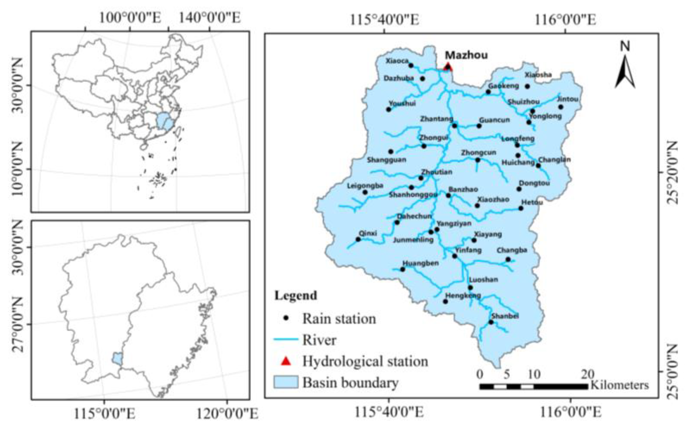
3.1. Study Area and Data

We tested the performance of the SA-CNN-LSTM model in the Mazhou Basin, Jiangxi Province, southeast China, which has a subtropical monsoon climate with high temperature and humidity. From March to June, frontal rain, sometimes persisting for >2 weeks, often occurs because of the influence of cold air moving from north to south. Typhoons, with heavy rainfall intensity, may affect the region from July to September. The Mazhou hydrological station (25°30′54′′N, 115°47′00′′E) was established in January 1958. It controls a basin area of 1758 km2, and the gradient of the main river is 1.53‰. The average annual flow at the Mazhou station is 47.3 m3/s, the average annual rainfall is 1560 mm, and the average annual evaporation is 1069 mm. The observation data used in this study include hourly precipitation data of 35 rainfall stations and the hourly runoff data of the Mazhou hydrological station, both acquired during the period of 2013–2021. The geographical location of the Mazhou watershed and the distribution of each station are shown in Figure 5.
The dataset was obtained by sliding the window in chronological order through the whole rainfall–runoff sequence. The size of the sliding window was set according to the timestep. The process of dataset preparation is shown in Figure 6. The dataset was divided into training and testing sets, which constituted 80% and 20% of the total records, respectively. The training set was used to calibrate the model parameters, whereas the testing set was used to evaluate model performance. To ensure consistent model input and enhance convergence speed during model training [63], the rainfall and streamflow were normalized before the training process:
D i N o r m = D i O r g D M I N O r g D M A X O r g D M I N O r g
where D i O r g is the original input data; D M A X and D M I N are the maximum and minimum values of the input data, respectively; and D i N o r m is the normalized input data.

3.2. Open-Source Software

This study relied on open-source libraries, including sklearn, NumPy, Math, and Matplotlib. Keras 2.1.5 and Python 3.7 were used to implement deep learning methods. The sklearn library was used to implement the random forest method. Matplotlib was used to draw figures. NumPy and Math were used for matrix operations. All experiments were conducted on a workstation equipped with an Intel E5-2680V3 CPU, 32 GB of RAM, and a NVIDIA GTX Geforce 2080 Ti GPU.

4. Results and Discussion

To explore the performance of the SA-CNN-LSTM model, four forecast models were compared: LSTM, CNN, ANN, and RF (random forest), along with the SA-LSTM and SA-CNN models. Additionally, SA-LSTM and SA-CNN models were used to discuss the impact of temporal and feature dependencies on runoff prediction respectively, and LSTM, CNN, ANN and RF were used as the benchmark models. Among these, the super-parameters of the CNN, LSTM, ANN, SA-LSTM, and SA-CNN models were optimized through the random search method; RF was set as the default recommended parameter.
In Section 4.1, the performance of the SA-CNN-LSTM model is compared with the performances of other models on the basis of different evaluation indicators. Comparisons of scatter plots and streamflow prediction in three categories are shown in Section 4.2 and Section 4.3, respectively. In Section 4.4, six selected flood events are used to evaluate the actual performance of the SA-CNN-LSTM model, compared with the performances of other models.

4.1. Comparisons of Evaluation Indicators

Comparisons of model performance according to evaluation indicator are shown in Table 2 and Table 3. The testing set result revealed that the prediction accuracy of each model decreased with increasing lead time. The SA-CNN-LSTM exhibited the best performance according to all evaluation indicators at the lead times of 1–5 h. Its performance at the lead times of 6–7 h was similar to the performances of the SA-LSTM and SA-CNN, although it remained better than the performance of the four benchmark models. From the results, the proposed model had better performance with short lead times, and the difference of indicators became smaller as the lead time increased. Notably, at the lead time of 1 h, the RMSE of the SA-CNN-LSTM was 51%, 55%, 61%, and 83% lower than the respective RMSE of the CNN, LSTM, ANN, and RF.
Comparison of performance among the four data-driven models revealed that RF performed the worst at each lead time, followed by ANN. This result indicated that the LSTM and CNN have a stronger ability to extract time series features, compared with ANN and RF, because of their specific network structures. At the lead times of 1–2 h, the predictive ability of the CNN was better than the predictive ability of the LSTM; subsequently, the performance of the LSTM was better. Tian et al. showed that whether a neural network model or a hydrological model is used for hydrological simulation, the basin with high station density will have more abundant data information and more accurate simulation results [64]. These above results may have occurred because the dense rainfall stations (50.25 km2/station) in the Mazhou watershed provided the CNN with rich rainfall features, which enhanced the prediction ability for the short forecast period. The LSTM exhibited outstanding forecast ability in the long forecast period because of its memory advantage in time series data.
In respective comparisons with the CNN and LSTM, the SA-CNN and SA-LSTM exhibited varying degrees of improved prediction accuracy with respect to the indicators. The RMSE of the SA-LSTM was 45% lower than the RMSE of the LSTM at the lead time of 1 h; the RMSE of the SA-CNN was 38% lower than the RMSE of the CNN at the lead time of 1 h. As indicated by the performances at different lead times, the SA-LSTM was always better than the LSTM as measured by the evaluation indicators; at the lead time of 7 h, it exhibited the best performance among all models. Notably, temporal dependencies improved the prediction performance of the LSTM, which was consistent with the conclusion of the articles proposed by Gao et al. [46,65] and Liu et al. [66]. However, their paper did not consider the impact of feature dependencies on runoff prediction. The SA-CNN had better prediction performance than the CNN only at the lead times of 1–2 h; it was less effective than the CNN at 3–7 h lead times. These results indicated that feature correlations help the CNN to perform better when predictions are made at a short lead time, but they have a negative effect on the CNN at longer lead times. This result may be related to the lack of memory ability of the CNN in time series, which leads to poor performance in more advanced prediction. However, the introduction of the self-attention mechanism increases model complexity and leads to reduced predictive ability. Based on the above results, temporal and feature dependencies can provide varying degrees of improvement in the predictive performances of conventional data-driven models. The self-attention mechanism has a more robust improvement effect on the LSTM, particularly in longer lead time forecasts; when combined with the self-attention mechanism, the CNN is more appropriate for short lead-time prediction, where it has better performance.
Chen et al. [46] developed the Self-Attentive Long Short-Term Memory (SA-LSTM), which achieved the best performance by comparing the four benchmark models, but the model only considered the temporal dependencies in the rainfall–runoff relationship and ignored importance of the feature dependencies. However, the SA-CNN-LSTM proposed by this study exhibited better comprehensive performance among all models in the prediction evaluation. This finding indicates that feature dependencies can further improve the prediction accuracy of the improved model considering only temporal dependencies, although its best performance only was observed with short lead times.

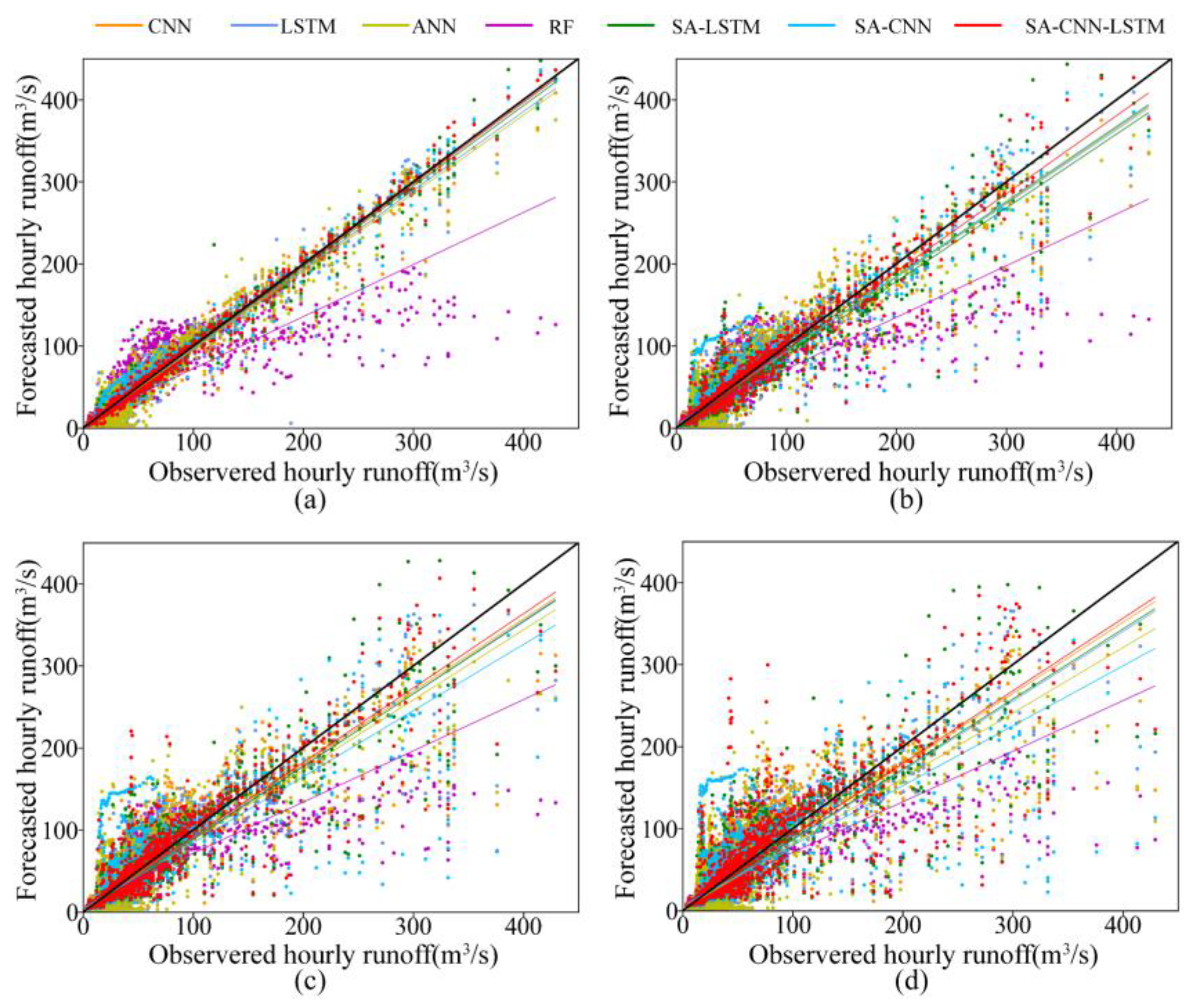
4.2. Comparison of Scatter Regression Plots

Figure 7 shows the scatter distributions of predicted and observed hourly runoff, along with the respective regression lines of each model, at lead times of 1, 3, 5, and 7 h. The regression line of the SA-CNN-LSTM is nearest to the ideal line (1:1) at different lead times, whereas RF is the model with the greatest deviation from the ideal line. At the lead time of 1 h, the ranking according to the distance from the ideal line is as follows: SA-CNN-LSTM < SA-CNN < SA-LSTM < LSTM < CNN < ANN < RF. This result indicates that the SA-CNN-LSTM model has the best forecasting ability, followed by the SA-CNN and SA-LSTM. However, the regression lines of the SA-CNN and SA-LSTM gradually fluctuate from the ideal line, indicating a lack of stability with increasing lead time. In contrast, the hybrid model integrating the CNN, LSTM, and the self-attention mechanism exhibits more stable performance. This result confirms that, after considering feature and temporal correlation, the combination of CNN, LSTM, and the self-attention mechanism has better robustness in terms of runoff prediction performance. The comparison of regression results further proves the importance of temporal and feature dependencies in improving runoff prediction.

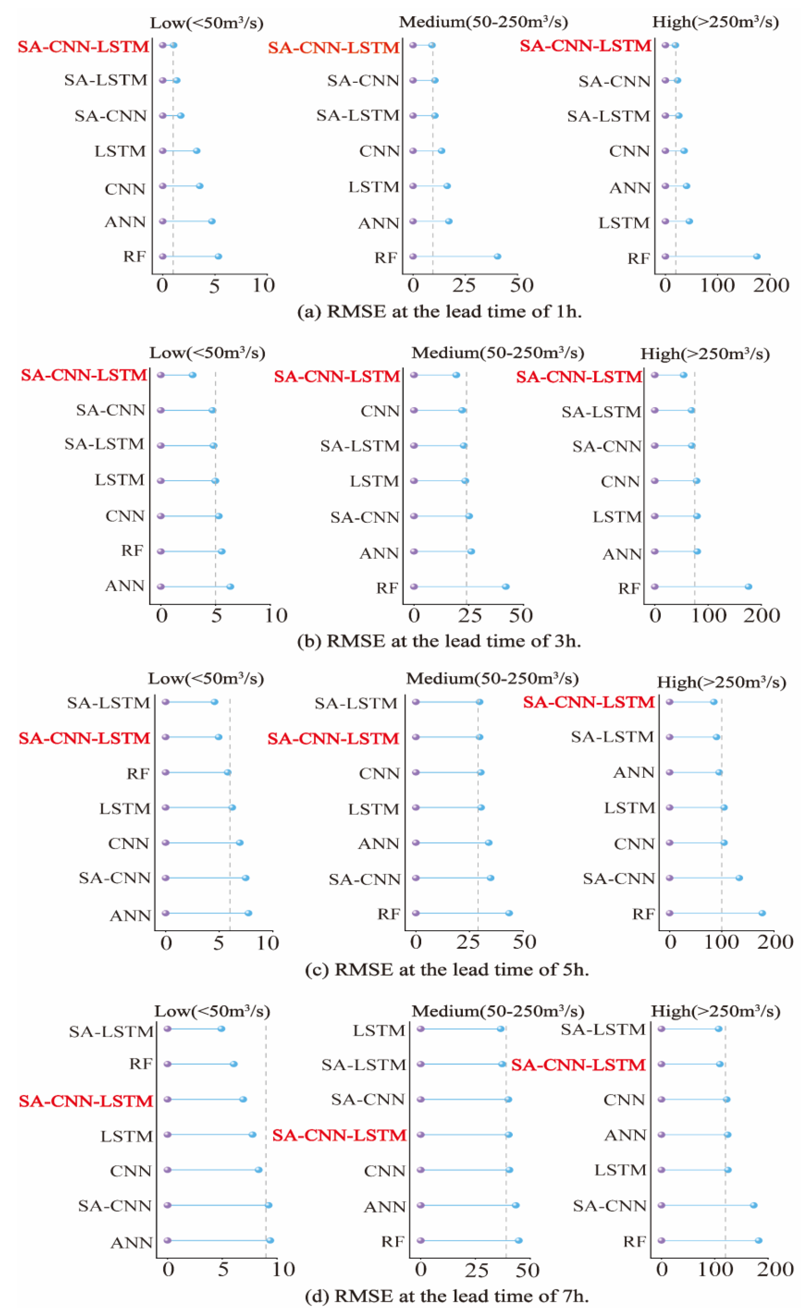
4.3. Comparisons of Streamflow in Three Categories

In terms of hydrology, high flow is important for flood forecasting, which can predict the impacts of potential floods and reduce the risks of economic loss. Low flow can affect the sustainable water supply for agricultural departments or groundwater recharge [67]. We divided streamflow into three categories according to flow value: low (0–50 m3/s), medium (50–250 m3/s), and high (>250 m3/s). We evaluated the performance of the SA-CNN-LSTM model with respect to prediction of streamflow in the different categories. Figure 8 shows the comparison of prediction results among models, according to RMSE, for the prediction periods of 1, 3, 5, and 7 h. The SA-CNN-LSTM exhibited excellent performance at various streamflow values. With increasing lead time, the model exhibited some degradation at low and medium flow values, but it maintained good performance at high flow values. These results indicate that the model is more stable with increasing lead time at high runoff flow values.

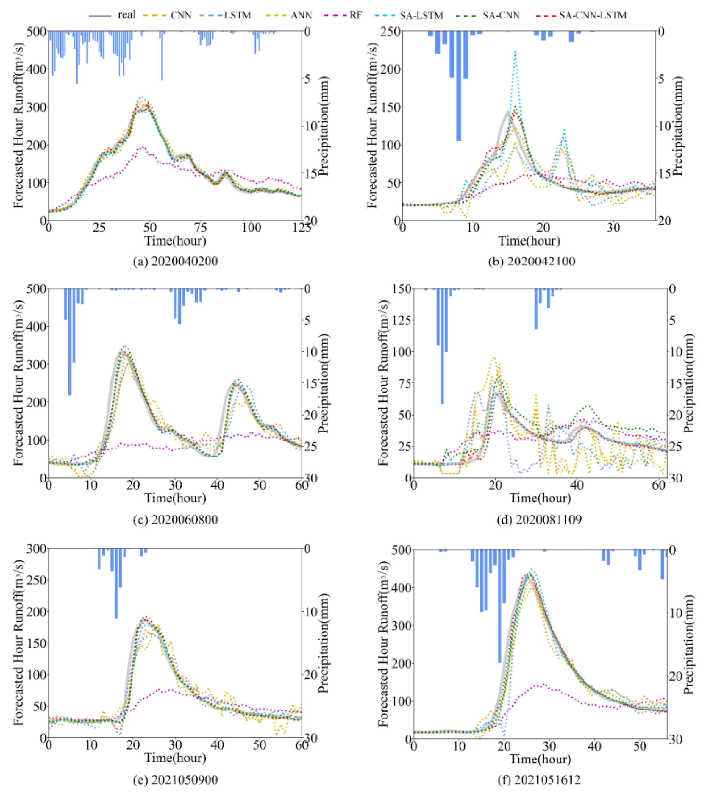
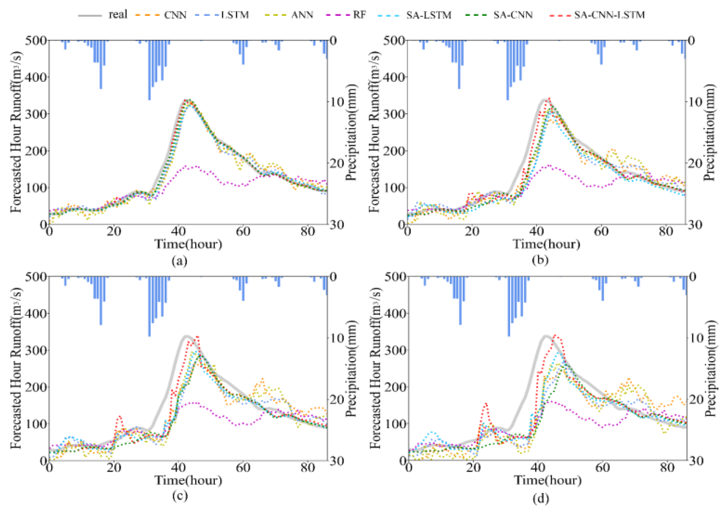
4.4. Comparisons of Performance during Actual Flood Events

As shown in Figure 9, six flood events were selected for evaluation of the SA-CNN-LSTM model’s performance during actual flood events; these events were 2020040200, 2020042100, 2020060800, 2020081109, 2021050900, and 2021051612. In addition, the evaluation indicators of these six floods were shown in Table 4, where PE was used to evaluate the performance of the flood peak predicted by the model. SA-CNN-LSTM showed the best performance in six flood events, and NSE of five floods was above 0.9. For the prediction of runoff peak, the PEs of SA-CNN-LSTM in six flood events were all within 3%, indicating that the flood peak prediction was also effective.
According to the flood process in Figure 9, the flood events 2021050900 and 2021051612 revealed that data-driven models exhibited some lag with respect to the observed peak time. However, the lag intervals of the SA-CNN-LSTM, SA-LSTM, and SA-CNN were smaller than the lag intervals of the other models. This finding indicates that the self-attention mechanism can alleviate the time lag in terms of flood peak prediction, which is a problem for conventional data-driven models. Among the models, the SA-CNN-LSTM had the best performance in terms of predicting peak time, further supporting its superiority. The flood event of 2020081109 was a small flood; the prediction results of the SA-CNN-LSTM in terms of flood rise and fall almost fully conformed to the observed values. Other comparison models exhibited poor performance. For the flood event of 2021051612, a high peak-value flood, the SA-CNN-LSTM performed better than other models in terms of flood peak time and peak value prediction. The performances for different magnitudes of flood indicated that the proposed model has good prediction performance in terms of peak line time, peak prediction, and flood rise and fall. In addition to flood peak prediction, base flow prediction is also important. For the flood events of 2021051612, 2021050900, and 2021051612, the SA-CNN-LSTM demonstrated good prediction of base flow, whereas other models exhibited some fluctuation. In summary, the proposed model was superior to other models in the prediction of actual flood events.
In order to verify the flood performance under different lead times, we also selected a new flood event (2021053000) to compare the model performance under different lead time, as shown in Figure 10. SA-CNN-LSTM performed well in simulating the flood peak in four different lead times, while the performance of other models on the peak value decreased with the increase of lead time. Table 5 showed the flood (2021053000) evaluation indicators of each model under different lead times. All the evaluation indicators of SA-CNN-LSTM was the best among all models at the lead times of 1, 3, 5, and 7 h. Especially in the lead time of 7 h, the PE of SA-CNN-LSTM was still within 3%. However, the PE of other comparison models all exceeded 10%. It can be predicted from the results that the proposed model also has certain potential in long lead times.

5. Conclusions

Previous research regarding data-driven models did not effectively exploit temporal and feature dependencies between time series elements. Therefore, we proposed a hybrid model, SA-CNN-LSTM, to improve streamflow prediction by considering temporal and feature dependencies. Our model combines the respective advantages of the CNN and LSTM to extract the characteristics of rainfall runoff; it uses a self-attention mechanism to improve performance and robustness by considering interdependence among timesteps and features. We tested the performance of the proposed model in the Mazhou Basin of China. To explore the performance of the SA-CNN-LSTM model, the LSTM, CNN, ANN, RF, SA-LSTM, and SA-CNN models were compared at lead times of 1–7 h. The SA-LSTM and SA-CNN models were used to discuss the impact of temporal and feature dependencies on runoff prediction respectively, and LSTM, CNN, ANN, and RF were used as the benchmark models.
The experimental results indicated that the SA-CNN-LSTM was better than the four benchmark models within the lead times of 1–7 h, especially in the lead times of 1–5 h, it had the best performance among all the comparison models, which is measured by various evaluation indicators. In addition, the base flow, peak value, and peak time flood prediction performances were partially improved. It can be proved that the combination of CNN, LSTM, and self-attention mechanism can more fully extract the abilities of input features, thereby improving prediction performance and model robustness. Respectively, temporal and feature dependencies can provide some degree of improvement regarding the predictive performances of conventional data-driven models (LSTM, CNN). The self-attention mechanism has a more robust improvement effect on the LSTM, particularly in forecasts with a longer lead time; when combined with the self-attention mechanism, the CNN is more appropriate for short lead-time prediction, where it has better performance. However, this study did not include an evaluation of model interpretability and cannot confirm the advantages of the model with respect to interpretability theory. In future research, we plan to focus on the combination of interpretability and the rainfall–runoff model.

Author Contributions

Conceptualization, F.Z. and Y.C.; methodology, F.Z.; software, F.Z.; validation, F.Z.; formal analysis, F.Z.; investigation, J.L.; resources, F.Z.; data curation, J.L.; writing—original draft preparation, F.Z.; writing—review and editing, Y.C; visualization, F.Z.; supervision, Y.C.; project administration, Y.C.; All authors have read and agreed to the published version of the manuscript.

Funding

This research was funded by the Science and Technology Program of Guangdong Province (no. 2020B1515120079), and the National Natural Science Foundation of China (NSFC) (no. 51961125206).

Data Availability Statement

Data sharing is not applicable.

Conflicts of Interest

The authors declare no conflict of interest.

References

  1. Liu, J.; Yuan, X.; Zeng, J.; Jiao, Y.; Li, Y.; Zhong, L.; Yao, L. Ensemble streamflow forecasting over a cascade reservoir catchment with integrated hydrometeorological modeling and machine learning. Hydrol. Earth Syst. Sci. 2022, 26, 265–278. [Google Scholar] [CrossRef]
  2. Yin, H.; Wang, F.; Zhang, X.; Zhang, Y.; Chen, J.; Xia, R.; Jin, J. Rainfall-runoff modeling using long short-term memory based step-sequence framework. J. Hydrol. 2022, 610, 127901. [Google Scholar] [CrossRef]
  3. Luo, P.; Liu, L.; Wang, S.; Ren, B.; He, B.; Nover, D. Influence assessment of new Inner Tube Porous Brick with absorbent concrete on urban floods control. Case Stud. Constr. Mater. 2022, 17, e01236. [Google Scholar] [CrossRef]
  4. Nourani, V.; Baghanam, A.H.; Adamowski, J.; Kisi, O. Applications of hybrid wavelet–Artificial Intelligence models in hydrology: A review. J. Hydrol. 2014, 514, 358–377. [Google Scholar] [CrossRef]
  5. Hu, R.; Fang, F.; Pain, C.; Navon, I. Rapid spatio-temporal flood prediction and uncertainty quantification using a deep learning method. J. Hydrol. 2019, 575, 911–920. [Google Scholar] [CrossRef]
  6. Luo, P.; Luo, M.; Li, F.; Qi, X.; Huo, A.; Wang, Z.; He, B.; Takara, K.; Nover, D.; Wang, Y. Urban flood numerical simulation: Research, methods and future perspectives. Environ. Model. Softw. 2022, 156, 105478. [Google Scholar] [CrossRef]
  7. Lin, Y.; Wang, D.; Wang, G.; Qiu, J.; Long, K.; Du, Y.; Xie, H.; Wei, Z.; Shangguan, W.; Dai, Y. A hybrid deep learning algorithm and its application to streamflow prediction. J. Hydrol. 2021, 601, 126636. [Google Scholar] [CrossRef]
  8. Lv, N.; Liang, X.; Chen, C.; Zhou, Y.; Li, J.; Wei, H.; Wang, H. A long Short-Term memory cyclic model with mutual information for hydrology forecasting: A Case study in the xixian basin. Adv. Water Resour. 2020, 141, 103622. [Google Scholar] [CrossRef]
  9. Scharffenberg, W.; Harris, J. Hydrologic Engineering Center Hydrologic Modeling System, HEC-HMS: Interior Flood Modeling. In Proceedings of the World Environmental and Water Resources Congress 2008, Honolulu, HI, USA, 12–16 May 2008; pp. 1–3. [Google Scholar]
  10. Chu, X.; Steinman, A. Event and Continuous Hydrologic Modeling with HEC-HMS. J. Irrig. Drain. Eng. 2009, 135, 119–124. [Google Scholar] [CrossRef]
  11. Zhang, S.; Zhou, Y. The analysis and application of an HBV model. Appl. Math. Model. 2012, 36, 1302–1312. [Google Scholar] [CrossRef]
  12. Ren-Jun, Z. The Xinanjiang model applied in China. J. Hydrol. 1992, 135, 371–381. [Google Scholar] [CrossRef]
  13. Baker, T.J.; Miller, S.N. Using the Soil and Water Assessment Tool (SWAT) to assess land use impact on water resources in an East African watershed. J. Hydrol. 2013, 486, 100–111. [Google Scholar] [CrossRef]
  14. Zhou, F.; Xu, Y.; Chen, Y.; Xu, C.-Y.; Gao, Y.; Du, J. Hydrological response to urbanization at different spatio-temporal scales simulated by coupling of CLUE-S and the SWAT model in the Yangtze River Delta region. J. Hydrol. 2013, 485, 113–125. [Google Scholar] [CrossRef]
  15. Abbott, M.; Bathurst, J.; Cunge, J.; O’Connell, P.; Rasmussen, J. An introduction to the European Hydrological System—Systeme Hydrologique Europeen, “SHE”, 1: History and philosophy of a physically-based, distributed modelling system. J. Hydrol. 1986, 87, 45–59. [Google Scholar] [CrossRef]
  16. Abbott, M.B.; Bathurst, J.C.; Cunge, J.A.; O’Connell, P.E.; Rasmussen, J. An introduction to the European Hydrological System—Systeme Hydrologique Europeen, “SHE”, 2: Structure of a physically-based, distributed modelling system. J. Hydrol. 1986, 87, 61–77. [Google Scholar] [CrossRef]
  17. Xu, S.; Chen, Y.; Xing, L.; Li, C. Baipenzhu Reservoir Inflow Flood Forecasting Based on a Distributed Hydrological Model. Water 2021, 13, 272. [Google Scholar] [CrossRef]
  18. Zhou, F.; Chen, Y.; Wang, L.; Wu, S.; Shao, G. Flood forecasting scheme of Nanshui reservoir based on Liuxihe model. Trop. Cyclone Res. Rev. 2021, 10, 106–115. [Google Scholar] [CrossRef]
  19. Chen, Y.; Li, J.; Xu, H. Improving flood forecasting capability of physically based distributed hydrological models by parameter optimization. Hydrol. Earth Syst. Sci. 2016, 20, 375–392. [Google Scholar] [CrossRef] [Green Version]
  20. Lees, T.; Buechel, M.; Anderson, B.; Slater, L.; Reece, S.; Coxon, G.; Dadson, S.J. Benchmarking data-driven rainfall–runoff models in Great Britain: A comparison of long short-term memory (LSTM)-based models with four lumped conceptual models. Hydrol. Earth Syst. Sci. 2021, 25, 5517–5534. [Google Scholar] [CrossRef]
  21. Yaseen, Z.M.; Sulaiman, S.O.; Deo, R.C.; Chau, K.-W. An enhanced extreme learning machine model for river flow forecasting: State-of-the-art, practical applications in water resource engineering area and future research direction. J. Hydrol. 2018, 569, 387–408. [Google Scholar] [CrossRef]
  22. Nearing, G.S.; Kratzert, F.; Sampson, A.K.; Pelissier, C.S.; Klotz, D.; Frame, J.M.; Prieto, C.; Gupta, H.V. What Role Does Hydrological Science Play in the Age of Machine Learning? Water Resour. Res. 2021, 57, e2020WR028091. [Google Scholar] [CrossRef]
  23. Xu, Y.; Hu, C.; Wu, Q.; Jian, S.; Li, Z.; Chen, Y.; Zhang, G.; Zhang, Z.; Wang, S. Research on particle swarm optimization in LSTM neural networks for rainfall-runoff simulation. J. Hydrol. 2022, 608, 127553. [Google Scholar] [CrossRef]
  24. Yokoo, K.; Ishida, K.; Ercan, A.; Tu, T.; Nagasato, T.; Kiyama, M.; Amagasaki, M. Capabilities of deep learning models on learning physical relationships: Case of rainfall-runoff modeling with LSTM. Sci. Total. Environ. 2021, 802, 149876. [Google Scholar] [CrossRef] [PubMed]
  25. Xie, K.; Liu, P.; Zhang, J.; Han, D.; Wang, G.; Shen, C. Physics-guided deep learning for rainfall-runoff modeling by considering extreme events and monotonic relationships. J. Hydrol. 2021, 603, 127043. [Google Scholar] [CrossRef]
  26. Montanari, A.; Rosso, R.; Taqqu, M.S. A seasonal fractional ARIMA Model applied to the Nile River monthly flows at Aswan. Water Resour. Res. 2000, 36, 1249–1259. [Google Scholar] [CrossRef]
  27. Wang, W.-C.; Chau, K.-W.; Xu, D.-M.; Chen, X.-Y. Improving Forecasting Accuracy of Annual Runoff Time Series Using ARIMA Based on EEMD Decomposition. Water Resour. Manag. 2015, 29, 2655–2675. [Google Scholar] [CrossRef]
  28. Rumelhart, D.E.; Hinton, G.E.; Williams, R.J. Learning representations by back-propagating errors. Nature 1986, 323, 533–536. [Google Scholar] [CrossRef]
  29. Riad, S.; Mania, J.; Bouchaou, L.; Najjar, Y. Predicting catchment flow in a semi-arid region via an artificial neural network technique. Hydrol. Process. 2004, 18, 2387–2393. [Google Scholar] [CrossRef]
  30. Khalil, A.F.; McKee, M.; Kemblowski, M.; Asefa, T. Basin scale water management and forecasting using artificial neural networks. JAWRA J. Am. Water Resour. Assoc. 2005, 41, 195–208. [Google Scholar] [CrossRef]
  31. Gao, S.; Huang, Y.; Zhang, S.; Han, J.; Wang, G.; Zhang, M.; Lin, Q. Short-term runoff prediction with GRU and LSTM networks without requiring time step optimization during sample generation. J. Hydrol. 2020, 589, 125188. [Google Scholar] [CrossRef]
  32. Van, S.P.; Le, H.M.; Thanh, D.V.; Dang, T.D.; Loc, H.H.; Anh, D.T. Deep learning convolutional neural network in rainfall–runoff modelling. J. Hydroinformatics 2020, 22, 541–561. [Google Scholar] [CrossRef] [Green Version]
  33. Chen, C.; Hui, Q.; Xie, W.; Wan, S.; Zhou, Y.; Pei, Q. Convolutional Neural Networks for forecasting flood process in Internet-of-Things enabled smart city. Comput. Networks 2020, 186, 107744. [Google Scholar] [CrossRef]
  34. Onan, A. Bidirectional convolutional recurrent neural network architecture with group-wise enhancement mechanism for text sentiment classification. J. King Saud Univ. Comput. Inf. Sci. 2022, 34, 2098–2117. [Google Scholar] [CrossRef]
  35. Liu, D.; Jiang, W.; Mu, L.; Wang, S. Streamflow Prediction Using Deep Learning Neural Network: Case Study of Yangtze River. IEEE Access 2020, 8, 90069–90086. [Google Scholar] [CrossRef]
  36. Feng, D.; Fang, K.; Shen, C. Enhancing Streamflow Forecast and Extracting Insights Using Long-Short Term Memory Networks With Data Integration at Continental Scales. Water Resour. Res. 2020, 56, e2019wr026793. [Google Scholar] [CrossRef]
  37. Xiang, Z.; Yan, J.; Demir, I. A Rainfall-Runoff Model With LSTM-Based Sequence-to-Sequence Learning. Water Resour. Res. 2020, 56, e2019wr025326. [Google Scholar] [CrossRef]
  38. Kratzert, F.; Klotz, D.; Herrnegger, M.; Sampson, A.K.; Hochreiter, S.; Nearing, G.S. Toward Improved Predictions in Ungauged Basins: Exploiting the Power of Machine Learning. Water Resour. Res. 2019, 55, 11344–11354. [Google Scholar] [CrossRef] [Green Version]
  39. Mao, G.; Wang, M.; Liu, J.; Wang, Z.; Wang, K.; Meng, Y.; Zhong, R.; Wang, H.; Li, Y. Comprehensive comparison of artificial neural networks and long short-term memory networks for rainfall-runoff simulation. Phys. Chem. Earth Parts A/B/C 2021, 123, 103026. [Google Scholar] [CrossRef]
  40. Granata, F.; Di Nunno, F.; de Marinis, G. Stacked machine learning algorithms and bidirectional long short-term memory networks for multi-step ahead streamflow forecasting: A comparative study. J. Hydrol. 2022, 613, 128431. [Google Scholar] [CrossRef]
  41. Kao, I.F.; Zhou, Y.; Chang, L.C.; Chang, F.J. Exploring a Long Short-Term Memory based Encoder-Decoder framework for multi-step-ahead flood forecasting. J. Hydrol. 2020, 583, 124631. [Google Scholar] [CrossRef]
  42. Cui, Z.; Qing, X.; Chai, H.; Yang, S.; Zhu, Y.; Wang, F. Real-time rainfall-runoff prediction using light gradient boosting machine coupled with singular spectrum analysis. J. Hydrol. 2021, 603, 127124. [Google Scholar] [CrossRef]
  43. Yin, H.; Zhang, X.; Wang, F.; Zhang, Y.; Xia, R.; Jin, J. Rainfall-runoff modeling using LSTM-based multi-state-vector sequence-to-sequence model. J. Hydrol. 2021, 598, 126378. [Google Scholar] [CrossRef]
  44. Chang, L.-C.; Liou, J.-Y.; Chang, F.-J. Spatial-temporal flood inundation nowcasts by fusing machine learning methods and principal component analysis. J. Hydrol. 2022, 612, 128086. [Google Scholar] [CrossRef]
  45. Ding, Y.; Zhu, Y.; Feng, J.; Zhang, P.; Cheng, Z. Interpretable spatio-temporal attention LSTM model for flood forecasting. Neurocomputing 2020, 403, 348–359. [Google Scholar] [CrossRef]
  46. Chen, X.; Huang, J.; Han, Z.; Gao, H.; Liu, M.; Li, Z.; Liu, X.; Li, Q.; Qi, H.; Huang, Y. The importance of short lag-time in the runoff forecasting model based on long short-term memory. J. Hydrol. 2020, 589, 125359. [Google Scholar] [CrossRef]
  47. Wang, Y.K.; Hassan, A. Impact of Spatial Distribution Information of Rainfall in Runoff Simulation Using Deep-Learning Methods. Hydrol. Earth Syst. Sci. 2021, 26, 2387–2403. [Google Scholar] [CrossRef]
  48. Zheng, Z.; Huang, S.; Weng, R.; Dai, X.-Y.; Chen, J. Improving Self-Attention Networks With Sequential Relations. IEEE/ACM Trans. Audio Speech Lang. Process. 2020, 28, 1707–1716. [Google Scholar] [CrossRef]
  49. Guo, M.-H.; Xu, T.-X.; Liu, J.-J.; Liu, Z.-N.; Jiang, P.-T.; Mu, T.-J.; Zhang, S.-H.; Martin, R.R.; Cheng, M.-M.; Hu, S.-M. Attention mechanisms in computer vision: A survey. Comput. Vis. Media 2022, 8, 331–368. [Google Scholar] [CrossRef]
  50. Yan, C.; Hao, Y.; Li, L.; Yin, J.; Liu, A.; Mao, Z.; Chen, Z.; Gao, X. Task-Adaptive Attention for Image Captioning. IEEE Trans. Circuits Syst. Video Technol. 2021, 32, 43–51. [Google Scholar] [CrossRef]
  51. Huang, B.; Liang, Y.; Qiu, X. Wind Power Forecasting Using Attention-Based Recurrent Neural Networks: A Comparative Study. IEEE Access 2021, 9, 40432–40444. [Google Scholar] [CrossRef]
  52. Alizadeh, B.; Bafti, A.G.; Kamangir, H.; Zhang, Y.; Wright, D.B.; Franz, K.J. A novel attention-based LSTM cell post-processor coupled with bayesian optimization for streamflow prediction. J. Hydrol. 2021, 601, 126526. [Google Scholar] [CrossRef]
  53. Sherstinsky, A. Fundamentals of Recurrent Neural Network (RNN) and Long Short-Term Memory (LSTM) Network. Phys. D Nonlinear Phenom. 2020, 404, 132306. [Google Scholar] [CrossRef] [Green Version]
  54. Mei, S.; Ji, J.; Hou, J.; Li, X.; Du, Q. Learning Sensor-Specific Spatial-Spectral Features of Hyperspectral Images via Convolutional Neural Networks. IEEE Trans. Geosci. Remote Sens. 2017, 55, 4520–4533. [Google Scholar] [CrossRef]
  55. Li, Q.; Chen, Y.; Zeng, Y. Transformer with Transfer CNN for Remote-Sensing-Image Object Detection. Remote. Sens. 2022, 14, 984. [Google Scholar] [CrossRef]
  56. Yao, G.; Lei, T.; Zhong, J. A review of Convolutional-Neural-Network-based action recognition. Pattern Recognit. Lett. 2018, 118, 14–22. [Google Scholar] [CrossRef]
  57. Wei, X.; Lei, B.; Ouyang, H.; Wu, Q. Stock Index Prices Prediction via Temporal Pattern Attention and Long-Short-Term Memory. Adv. Multimedia 2020, 2020, 8831893. [Google Scholar] [CrossRef]
  58. Shih, S.-Y.; Sun, F.-K.; Lee, H.-Y. Temporal pattern attention for multivariate time series forecasting. Mach. Learn. 2019, 108, 1421–1441. [Google Scholar] [CrossRef] [Green Version]
  59. Wilson, A.C.; Roelofs, R.; Stern, M.; Srebro, N.; Recht, B. The Marginal Value of Adaptive Gradient Methods in Machine Learning. arXiv 2014. [Google Scholar] [CrossRef]
  60. Leslie, N.; Smith, N.T. Super-Convergence: Very Fast Training of Neural Networks Using Large Learning Rates. arXiv 2017. [Google Scholar] [CrossRef]
  61. Shamseldin, A.Y. Application of a neural network technique to rainfall-runoff modelling. J. Hydrol. 1997, 199, 272–294. [Google Scholar] [CrossRef]
  62. Krause, P.; Boyle, D.P.; Bäse, F. Comparison of different efficiency criteria for hydrological model assessment. Adv. Geosci. 2005, 5, 89–97. [Google Scholar] [CrossRef] [Green Version]
  63. Sergey Ioffe, C.S. Batch Normalization: Accelerating Deep Network Training by Reducing Internal Covariate Shift. arXiv 2015. [Google Scholar] [CrossRef]
  64. Tian, Y.; Xu, Y.-P.; Yang, Z.; Wang, G.; Zhu, Q. Integration of a Parsimonious Hydrological Model with Recurrent Neural Networks for Improved Streamflow Forecasting. Water 2018, 10, 1655. [Google Scholar] [CrossRef] [Green Version]
  65. Gao, S.; Zhang, S.; Huang, Y.; Han, J.; Luo, H.; Zhang, Y.; Wang, G. A new seq2seq architecture for hourly runoff prediction using historical rainfall and runoff as input. J. Hydrol. 2022, 612, 128099. [Google Scholar] [CrossRef]
  66. Liu, Y.; Zhang, T.; Kang, A.; Li, J.; Lei, X. Research on Runoff Simulations Using Deep-Learning Methods. Sustainability 2021, 13, 1336. [Google Scholar] [CrossRef]
  67. Li, Y.; Wang, G.; Liu, C.; Lin, S.; Guan, M.; Zhao, X. Improving Runoff Simulation and Forecasting with Segmenting Delay of Baseflow from Fast Surface Flow in Montane High-Vegetation-Covered Catchments. Water 2021, 13, 196. [Google Scholar] [CrossRef]
Figure 1. LSTM structure.
Remotesensing 15 01395 g001
Figure 2. One-dimensional convolution operation process.
Remotesensing 15 01395 g002
Figure 3. Flowchart of SA-CNN-LSTM model.
Remotesensing 15 01395 g003
Figure 4. Correlation coefficients between rainfall and runoff.
Remotesensing 15 01395 g004
Figure 5. Location of the Mazhou Basin (China) and distribution of stations in the basin.
Remotesensing 15 01395 g005
Figure 6. Process of dataset preparation.
Remotesensing 15 01395 g006
Figure 7. Scatter plots and fitting lines of prediction results for each model at lead times of 1 (a), 3 (b), 5 (c), and 7 (d) h.
Remotesensing 15 01395 g007
Figure 8. Comparisons of streamflow predictions in three categories of flow for each model at lead times of 1, 3, 5, and 7 h.
Remotesensing 15 01395 g008
Figure 9. Comparisons of the predictions from each model with a lead time of 1 h.
Remotesensing 15 01395 g009
Figure 10. Comparisons of the predictions of the flood event (2021053000) from each model at the lead times of 1 (a), 3 (b), 5 (c), and 7 (d) h.
Remotesensing 15 01395 g010
Table 1. Ranges of model super-parameters used in optimization.
Super-ParameterRange
LSTM layer8–256
Autoregressive layer8–256
CNN layer8–256
Attention layer8–256
Learning rate[0.1, 0.01, 0.001, 0.0001, 0.00001]
Table 2. Performances of each model in the training set.
Model/TrainLead Time of 1 hLead Time of 2 hLead Time of 3 h
NSEMAEMRERMSENSEMAEMRERMSENSEMAEMRERMSE
CNN0.9961.9410.1413.4240.9922.8550.2434.4770.9903.2780.2605.283
LSTM0.9942.1780.1633.8940.9913.0170.2224.9100.9902.9850.1975.217
ANN0.9942.5550.2224.0730.9912.9790.2344.8530.9903.1330.2495.062
RF0.9742.2340.0908.3400.9742.2600.0918.3360.9742.2860.0938.341
SA-CNN0.9931.1820.0344.2730.9861.8730.0616.1370.9762.5750.0868.002
SA-LSTM0.9941.1860.0353.8350.9892.2610.0995.3280.9734.9180.2418.439
SA-CNN-LSTM0.9941.3440.0593.9200.9901.7830.0565.2140.9852.5250.0996.343
Model/TrainLead Time of 4 hLead Time of 5 hLead Time of 6 h
NSEMAEMRERMSENSEMAEMRERMSENSEMAEMRERMSE
CNN0.9863.6740.2756.0560.9834.0310.2876.8300.9764.5720.3047.950
LSTM0.9883.4570.2555.7100.9853.4790.2256.3020.9814.0920.2837.065
ANN0.9903.2840.2575.2360.9893.4030.2615.3770.9873.6530.2695.901
RF0.9742.3140.0948.3650.9732.3440.0968.4090.9732.3820.0988.511
SA-CNN0.9653.0800.0779.7040.9503.8590.11011.5120.8685.0480.16618.742
SA-LSTM0.9793.1620.1257.4040.9723.9800.1318.5670.9664.4960.1629.544
SA-CNN-LSTM0.9802.8660.0827.2230.9763.4910.1437.9700.9724.0500.2098.703
Model/TrainLead Time of 7 h
NSEMAEMRERMSE
CNN0.9714.7700.3068.812
LSTM0.9774.3720.2927.844
ANN0.9844.0980.2836.582
RF0.9722.4280.1008.635
SA-CNN0.9264.9970.21714.074
SA-LSTM0.9634.5800.1939.965
SA-CNN-LSTM0.9674.5540.2599.437
Table 3. Performances of each model in the testing set.
Model/TestLead Time of 1 hLead Time of 2 hLead Time of 3 h
NSEMAEMRERMSENSEMAEMRERMSENSEMAEMRERMSE
CNN0.9652.6390.1364.9780.9362.9710.1346.7080.8993.7010.1678.441
LSTM0.9581.9690.0815.4160.9263.5130.1787.2190.8993.4980.1608.441
ANN0.9432.8110.1236.3070.9113.6930.1687.9280.8784.1500.1839.256
RF0.6964.3330.13614.6260.6904.4470.14114.7720.6844.5600.14614.918
SA-CNN0.9870.8260.0293.0800.9541.4200.0485.6640.8992.0610.0678.452
SA-LSTM0.9870.7990.0292.9720.9591.8790.0825.3460.9124.2570.2127.885
SA-CNN-LSTM0.9920.9010.0412.4350.9741.2370.0464.2710.9501.5980.0565.914
Model/TestLead Time of 4 hLead Time of 5 hLead Time of 6 h
NSEMAEMRERMSENSEMAEMRERMSENSEMAEMRERMSE
CNN0.8554.3290.19110.1130.8214.9380.21811.2200.7635.8760.26112.907
LSTM0.8653.6430.1499.7380.8333.8600.15010.8310.7875.2060.23412.231
ANN0.8404.7200.20810.6220.8015.0070.21211.8250.7485.5850.23213.316
RF0.6774.6720.15115.0830.6704.7800.15615.2500.6614.8930.16115.456
SA-CNN0.8292.7530.09310.9620.7553.3200.11213.1340.7792.8510.09112.478
SA-LSTM0.9092.2220.0767.9960.8753.4540.1439.3750.8533.2930.12210.169
SA-CNN-LSTM0.9172.2720.0837.6660.8752.5110.0849.3730.8342.9210.10010.818
Model/TestLead Time of 7 h
NSEMAEMRERMSE
CNN0.7275.9740.25113.868
LSTM0.7545.6500.25613.163
ANN0.6856.6900.29314.901
RF0.6495.0130.16615.719
SA-CNN0.6254.2040.14016.247
SA-LSTM0.8223.2600.11111.195
SA-CNN-LSTM0.7743.3950.11812.615
Table 4. Comparisons of evaluation indicators of six flood events from each model at the lead time of 1 h.
Flood SA-CNN-LSTMSA-LSTMSA-CNNLSTMCNNANNRF
2020040200NSE0.990.990.990.980.990.980.55
MAE4.865.984.887.366.427.7139.41
MRE0.040.050.040.060.050.060.29
RMSE6.497.886.229.728.8410.3150.82
PE
(305.6 m3/s)
1.7%
(311.04)
5%
(290.14)
2.2%
(298.82)
7%
(327.15)
1.6%
(310.54)
3%
(314.78)
36.4%
(195.23)
2020042100NSE0.870.310.850.450.750.350.21
MAE5.9711.985.9213.2210.0415.7215.67
MRE0.090.190.080.230.220.290.23
RMSE10.5624.6311.5722.0214.9023.8926.45
PE
(144 m3/s)
0.1%
(144.21)
55%
(223.7)
4.6%
(150.76)
24.6%
(108.49)
14.4%
(123.2)
27.7%
(104.01)
57%
(61.84)
2020060800NSE0.940.930.930.800.870.79−0.15
MAE11.8012.3212.6523.5418.5526.6860.45
MRE0.080.080.090.200.170.260.38
RMSE21.0722.0422.4637.2529.9737.9789.68
PE
(331.6 m3/s)
0.2%
(332.55)
1.9%
(325.18)
5.5%
(351.1)
8.2%
(304.35)
1%
(328.1)
5.7%
(312.42)
63.3%
(121.59)
2020081109NSE0.910.830.49−0.870.08−0.830.35
MAE2.142.778.9414.8210.2614.899.24
MRE0.080.130.340.580.400.580.37
RMSE4.365.8610.1719.4313.6119.2211.47
PE
(67.33 m3/s)
2.1%
(68.76)
0.02%
(67.31)
18.9%
(80.11)
12.8%
(77.29)
33.5%
(89.9)
42%
(95.65)
29.9%
(47.14)
2021050900NSE0.960.950.960.940.910.890.26
MAE4.074.774.258.469.9411.7623.06
MRE0.060.070.060.160.180.220.26
RMSE9.6510.779.9111.8714.5216.3842.06
PE
(186.6 m3/s)
1%
(188.58)
4.2%
(178.61)
3.1%
(192.41)
10.9%
(166.17)
4.8%
(177.52)
6.9%
(173.74)
58.5%
(77.34)
2021051612NSE0.990.980.980.900.960.950.19
MAE7.068.709.2719.1213.8818.6565.50
MRE0.060.060.070.150.150.160.31
RMSE11.7716.7417.8339.4523.3328.41110.34
PE
(429.1 m3/s)
1.7%
(436.48)
4.3%
(447.88)
1%
(433.61)
1.6%
(436.55)
3%
(415.83)
6.7%
(400.31)
65.8%
(146.4)
Table 5. Comparisons of evaluation indicators of flood event (2021053000) from each model at the lead times of 1, 3, 5, and 7 h.
Lead Time SA-CNN-LSTMSA-LSTMSA-CNNLSTMCNNANNRF
1 hNSE0.990.980.990.960.960.950.35
MAE4.407.894.6711.5513.4915.3944.65
MRE0.040.060.040.100.130.160.24
RMSE7.3212.838.1017.8018.4520.1870.24
PE
(336.8 m3/s)
0.01%
(336.85)
4.4%
(321.98)
0.7%
(339.38)
4.1%
(322.78)
1.1%
(332.89)
1.1%
(332.88)
52.6%
(159.35)
3 hNSE0.950.830.910.860.850.860.32
MAE12.2823.6314.2620.9324.5824.6746.29
MRE0.110.190.110.170.210.240.25
RMSE19.5635.8525.7033.0734.2132.7871.64
PE
(336.8 m3/s)
1.5%
(342.01)
9.8%
(303.75)
5%
(319.87)
8.9%
(306.63)
15%
(286.23)
7.7%
(310.86)
51.5%
(163.19)
5 hNSE0.860.780.740.710.690.700.29
MAE20.9625.1325.4829.6235.9233.4848.53
MRE0.190.200.190.230.300.290.27
RMSE32.2140.9644.7047.1648.1747.6973.58
PE
(336.8 m3/s)
1%
(340.22)
11.8%
(296.76)
15.1%
(285.69)
15.1%
(285.90)
21.8%
(263.25)
12.6%
(294.19)
52.5%
(159.72)
7 hNSE0.770.690.500.550.480.490.23
MAE27.4330.0834.9835.7048.8944.3850.76
MRE0.240.240.240.260.410.390.28
RMSE42.1948.8161.4158.5663.0262.0676.50
PE
(336.8 m3/s)
1.3%
(341.42)
13.4%
(291.59)
22.5%
(260.80)
19.8%
(269.93)
27.6%
(243.62)
21.4%
(264.51)
52.3%
(160.60)
Disclaimer/Publisher’s Note: The statements, opinions and data contained in all publications are solely those of the individual author(s) and contributor(s) and not of MDPI and/or the editor(s). MDPI and/or the editor(s) disclaim responsibility for any injury to people or property resulting from any ideas, methods, instructions or products referred to in the content.

