Absolute Calibration of the Chinese HY-2B Altimetric Mission with Fiducial Reference Measurement Standards

Abstract

This research and collaboration work aims at the calibration and validation (Cal/Val) of the Chinese HY-2B satellite altimeter based upon two permanent Cal/Val facilities: (1) the China Altimetry Calibration Cooperation Plan in Qingdao, Bohai Sea and the Wanshan islands, China and (2) the permanent facility for altimetry calibration established by the European Space Agency in Crete, Greece. The HY-2B satellite altimeter and its radiometer have been calibrated and monitored using uniform, standardized procedures, as well as protocols and best practices, and they also built upon trusted and indisputable reference standards at both Cal/Val infrastructures in Europe and China. The HY-2B altimeter is thus monitored in a coordinated, absolute, homogeneous, long-term and worldwide manner. Calibration of altimeters is accomplished by examining satellite observations in open seas against reference measurements. Comparisons are established through precise satellite positioning, water level observations, GPS buoys and reference models (geoid, mean dynamic topography, earth tides, troposphere and ionosphere), all defined at the Cal/Val sites. In this work, the final uncertainty for the altimeter bias will be attributed to several individual sources of uncertainty, coming from observations in water level, atmosphere, absolute positioning, reference surface models, transfer of heights from Cal/Val sites to satellite observations, etc. Through this project, the procedures, protocols and best practices, originally developed in the course of the ESA FRM4ALT project, are updated, upgraded and followed at both Cal/Val facilities in Europe and China. All in all, the HY-2B satellite altimeter observes the sea level quite well and within its specifications.

1. Introduction

The compelling environmental challenge humanity faces at present is climate change. To assess its impact, and especially that part induced by human activities, it requires continuous, indisputable, long standing and accurate monitoring of all hydrological, oceanic, atmospheric and geophysical variations caused by climate change at a global scale. One of the most important climate change indicators is the global mean sea level, as it directly threatens communities living around coastal regions and small islands (e.g., at a low elevation of less than 10 m) [1]. Moreover, climate change can cause extreme weather events that also impact the well-being and security of communities living further from the coast [2].

Global monitoring and assessment of the sea level rise is performed primarily by satellite altimetry. After more than four decades of operations and about 20 missions, satellite altimetry products are essential for any Earth observations program [3]. Altimetric satellites are designed to provide accurate measurements of various geophysical parameters related to the ocean state, near-coast sea state [4], inland waters [5] and ice caps’ monitoring. Some examples of products derived from altimetric observations are sea surface height, wave height, wind speed [6], ionospheric total electron content [7], sea and land ice coverage [8], and polar region topography [9]. On 21 November 2020, the current family of operational satellite altimetry missions (i.e., Sentinel-3A/3B, Jason-3, CryoSat-2, ICESat-2 and HY-2B/2C) welcomed its eighth member: the Copernicus Sentinel-6 Michael Freilich (MF) satellite mission [10]. The successful launch and operation of the Sentinel-6 MF satellite ensures the uninterrupted monitoring of the oceanic environment and acquisition of an accurate set of ocean observations. On 15 December 2022, the new US-French interferometric satellite SWOT [11] was also placed in orbit.

To successfully understand, prevent and mitigate the environmental and security risks caused directly or indirectly by climate change, bilateral as well as multilateral partnerships have been realized [12]. One such partnership, called the Dragon Program, among the European Space Agency (ESA), the Ministry of Science and Technology (MOST) of China and the National Remote Sensing Center of China (NRSCC) has been established since 2004.

The Dragon research initiative supports joint research activities between European and Chinese institutes, who exploit data from Earth observations using satellites. The sea level rise and coastal zone management along with calibration and validation (Cal/Val) of satellite products constitute two of the priorities of the ongoing Dragon 5 program.

Calibration and validation are fundamental and prerequisite to the successful operation of any satellite altimeter. They constitute a major task in all Earth observations and are routinely performed during Commissioning and throughout a satellite’s normal operation. The in-flight accuracy of both satellite observations and their associated geophysical products is accessed not only by the operating agencies, but also by external, independent and international research teams. High quality for the satellite observations establishes and leads to confidence and accuracy on the information presented to the public and assists policymakers towards proper decisions for mitigating the effects caused by climate change [13].

Along the lines of confidence building, the strategy for Fiducial Reference Measurements for Altimetry (FRM4ALT) was established by ESA. It leads to trustworthy measures and tools towards a uniform and absolute standardization for Cal/Val activities in satellite altimetry. Likewise, the Dragon 5 project (ID-59198, named FRM4ALT@CN) aims at bringing reliable measures and procedures for establishing Cal/Val uncertainty budgets, capable of being traced to metrology standards. Such procedures apply also to the two permanent Cal/Val sites in Europe and China and for all existing and upcoming European and Chinese satellite altimeters.

This paper presents the first joint Cal/Val results for the HY-2B satellite altimeter determined at the permanent Cal/Val sites in western Crete, Greece and in the Qingdao, Bohai Sea and Wanshan islands realized though the China Altimetry Calibration Cooperation Plan. The absolute calibration of the HY-2B altimeter was carried out by estimating its bias based upon sea level observations around the Cal/Val sites. The cross-calibration of HY-2B against Jason-3 and Sentinel-3A/3B is also performed at crossover points at sea. Finally, the Cal/Val of HY-2B geophysical products and its on-board instrumentation is complemented with an assessment of the HY-2B radiometric measurements to determine its radiometer bias.

Section 2 of this paper presents the key characteristics of the HY-2B satellite, and the infrastructure and instrumentation of the permanent Cal/Val sites operating since 2008 at the west coast of Crete and since 2018 in China. Section 3 provides information regarding the data sets (i.e., altimetric products, tide-gauge and positioning time series) used for the calibration of HY-2B. In Section 4, a detailed review of the Cal/Val methodologies is presented, which are employed to evaluate the performance of HY-2B.

The estimation of the Cal/Val uncertainty budget, following the FRM4ALT action plan [13], is also given. The uncertainty constituents and major sources of uncertainty are also examined, i.e., wet tropospheric delay and reference surfaces. The results of the absolute bias, relative bias and uncertainty budget analysis are presented in Section 5. Finally, a discussion of the results and the most important conclusions of this work are provided in Section 6 along with a description of future plans towards the accomplishment of the Dragon-5 research objectives.

2. The HY-2B Altimeter Satellite

The HY-2B altimeter was operated by the National Satellite Ocean Application Service (NSOAS). It is China’s second satellite altimetry mission and is dedicated to the spatio-temporal monitoring of the marine dynamic environment. Its launch was carried out by the China National Space Administration (CNSA) at the Taiyuan Satellite Launch Center using a Chang Zheng 4B carrier rocket [14] on 25 October 2018.

The orbit of the HY-2B satellite is sun-synchronous with an altitude of about 970 km and an inclination of 99.34${}^{\circ }$ (almost a polar orbit). The spacecraft was originally scheduled to maintain a 14-day period for oceanic applications in the first two years of its lifetime, and an 168-day period for geodetic applications afterwards [15,16]. Because of its high performance, the satellite still follows its oceanographic orbit with a period of 14 days.

The primary scientific objectives of HY-2B are to measure and monitor parameters which describe the marine dynamic environment, such as sea surface and significant wave height, sea-surface wind and sea-surface temperature [17]. The knowledge of how these parameters evolve in time and on a global scale has been proven to be beneficial for several disciplines, including oceanography, physical geodesy and climate change research.

In order to meet its end objectives, the HY-2B spacecraft is equipped with four main instruments: a dual-frequency radar altimeter operating in Ku and C bands, a Ku-band dual-point pencil beam rotating radar scatterometer, a five-band scanning microwave radiometer and a correction microwave radiometer. The radar altimeter is used for the estimation of sea-surface height and significant wave height by analyzing the mean return waveform of a repeatedly transmitted electromagnetic pulse [18,19,20]. The use of a dual-band altimetric system also allows the estimation of ionospheric delay corrections. More information on the HY-2B altimeter specifications can be found in [21]. Observations derived from the radar scatterometer are used in the estimation of sea-surface wind fields [22,23,24]. The scanning microwave radiometer is used for the estimation of sea-surface temperature [17,25] and the correction microwave radiometer for the estimation of tropospheric delay corrections. Precise orbit determination of HY-2B is also possible via Satellite Laser Ranging (SLR) and dual-frequency Global Navigation Satellite System (GNSS) tracking.

A major technological development since HY-2B’s predecessor mission, HY-2A, is the use of a rubidium atomic clock as a frequency reference that ensures an altimetric range drift of less than 0.1 mm/yr [21]. An assessment of the HY-2B satellite altimeter against Jason-2/3 altimeters demonstrated that the former already has more stable performance and a smaller noise level than the latter, whereas, all three missions produce significant wave heights of comparable accuracy [15]. The follow-up missions, HY-2C and HY-2D, are also part of China’s marine dynamic satellite constellation program, with the former one launched on 21 September 2020, and the latter one on 19 May 2021.

3. The Cal/Val Infrastructures

3.1. The Permanent Facility for Altimeter Calibration in Europe

The Permanent Facility for Altimeter Calibration (PFAC) in western Crete, Greece, is one of the few permanent facilities in the world dedicated to multi-mission satellite altimetry Cal/Val activities. Figure 1 shows the Cal/Val site distribution over the Crete and Gavdos islands and in relation to the Sentinel-3, Jason-3, HY-2B, SWOT [11] and Sentinel-6A MF ground track coverage.

Since its establishment in 2004, the PFAC has been providing Cal/Val results for all international altimetry missions, such as Jason-1/2/3, Sentinel-3A/B, SARAL/AltiKa and HY-2A [26]. Currently, its activities have been extended to the calibration of the tandem mission of Jason-3 with Sentinel-6A (Michael Freilch) during its Commissioning, CryoSat-2, HY-2B and certainly calibration, and, later on, of the operational satellite of Sentinel-6A MF.

The PFAC consists of four permanent sea-surface Cal/Val sites, namely, the GVD8 site at Gavdos island and the CRS1, SUG1 and RDK1 sites in southwestern Crete. Two additional Cal/Val sites (KLM1 and KRM1) are currently under construction. This infrastructure also includes two fully operational transponder Cal/Val sites at the Ku-band, namely, the CDN1 Cal/Val site located on a mountainous region in the western part of Crete [27] and the recently established GVD1 Cal/Val site on Gavdos island.

Coastal Cal/Val sites are primarily used for the absolute and relative sea-surface calibration of altimeters. Each site is commonly equipped with at least two sets of continuously operating instrumentation, such as tide-gauges, permanent GNSS stations, meteorological sensors, etc. The transponder Cal/Val sites are used for the absolute range and datation (time-tagging) altimeter calibration. They are likewise equipped with a microwave transponder and at least two units of permanent GNSS stations, meteorological sensors, power supply units, communication links, etc.

The location of each Cal/Val site is strategically selected to allow for the calibration of all operational satellite altimeters and with redundancy. These sites are also meant to support the calibration of future missions, such as CRISTAL [28], SWOT [11], Quanlan [29], etc. The spatial extent of the PFAC network also allows for the calibration of multiple satellites in ascending and descending passes.

Apart from the Cal/Val sites, an independent network of continuously operating GNSS stations (called the TUC Network) has also been established in western Crete and operating continuously since 2001 [30]. The TUC network acts as an infrastructure to monitor tectonic deformations and to support the regional Cal/Val operations. The same network also upholds the estimation of the ionospheric and wet tropospheric delays used for reducing satellite altimetry signals.

In the present work, the CRS1 and RDK1 sea-surface Cal/Val sites were selected for the calibration of the HY-2B Chinese satellite altimeter, as they were in proximity to the satellite’s groundtracks. Specifically, the CRS1 Cal/Val site is used for the calibration of HY-2B’s descending pass No. 66 (i.e., D66, D = Descending). The same site is also operated for the calibration of Sentinel-3A (D278) and Sentinel-3B (A14, A = Ascending) satellites (Figure 2a). Moreover, the other Cal/Val site of RDK1 facilitates the calibration of HY-2B’s ascending pass No. 161 (A161) and also that of Sentinel-3A (pass D335), Sentinel-3B (pass A71) and Jason-3/Sentinel-6A MF (pass A109) (Figure 2b).

The CRS1 Cal/Val site is equipped with two tide-gauges, called SVR1 and SVR2, and which operate on different measuring principles, i.e., pressure and radar, respectively. The cross-examination of water level determination using this setup with different and independent instruments and principles ensures a robust estimation of the sea-surface height. Moreover, observations from a permanent GNSS station and a meteorological sensor on site complement the tide-gauge measurements and contribute to the Cal/Val process.

The CRS1 infrastructure is illustrated in Figure 3 and its instruments’ main characteristics are given in

Table 1. Main instrument characteristics at the CRS1 sea-surface Cal/Val site.

Name	Type	Description
CRS1	GNSS system	Leica GRX1200GG PRO receiver
		Leica AT504 Choke Ring Antenna
CRS1	Meteorological station	Vaisala PTU-300
SVR1	Pressure tide-gauge	Valeport Tidemaster
SVR2	Radar tide-gauge	OTT Radar Level Sensor

. The other RDK1 Cal/Val site (Figure 4) is equipped with two radar tide-gauges, named RDN1 and RDN2, and its permanent GNSS station, meteorological sensors, etc.

3.2. The Altimetry Calibration Cooperation Plan of China

China has already built the ground infrastructure for calibrating satellite altimeters (Figure 5). It is established to help produce reliable and long-term HY-2 altimeter records, by calibrating altimeter observations mainly using the ground framework at the Wanshan Cal/Val site. This ground infrastructure has been called the Altimetry Calibration Cooperation Plan (ACCP) of China, and partners of the ACCP could freely use the in situ data [31].

As shown in Figure 5, the Wanshan Cal/Val site (“Wanshan” literally means thousand hills in Chinese) is located in the southern waters of Hong Kong and adjacent to the South China Sea. The main area of this Cal/Val site is about 20 km south from the Wanshan Archipelago on the South China Sea, located at the outermost side of the Pearl River Estuary. Its average sea depth is no more than 40 m. Its first dedicated site in Wanshan was built in 2019 for calibrating the HY-2 series satellite altimetry missions, including HY-2B and HY-2C.

At present, various calibration facilities have been established at the Wanshan Cal/Val site, including four GNSS receivers, three acoustic tide-gauges, one automatic weather station, one solar photometer and one mooring tide-gauge. Moreover, the Data Reception and Maintenance Center in the Guishan Island is established for the collection, evaluation, analysis, management and transmission of calibration and ground reference data.

The deployment and the usage of these ground calibration facilities are as follows: (1) Four GNSS receivers established, respectively, in the Wailingding Island (some of its instrumentation are shown in Figure 6), the Dangan Island, the Zhiwan Island and the Miaowan Island, provide the water level reference for the collocated tide-gauges, and the tropospheric and the ionospheric signal delays; (2) three acoustic tide-gauges set up on the islands of Wailingding, Dangan and Zhiwan, produce observation data of the sea level for the calibration process; (3) an automatic weather station and solar photometer in Dangan Island supplies ambient parameters of the atmosphere, such as wind, atmospheric pressure, air temperature, water vapor and other auxiliary parameters for tropospheric correction validation; and finally, (4) the mooring tide-gauge is placed 50 km south of the island at the sub-satellite point under the ascending track No. 375 of HY-2B (A375). This provides the direct sea level observation data. In the future, a GNSS buoy is to be placed on the cross track of HY-2B and HY-2C as part of the Altimetry Calibration Cooperation Plan.

4. Datasets, Quality Control and FRM Uncertainty

This section describes the procedure for the calculation of the FRM uncertainty at the CRS1 and RDK1 Cal/Val sites. The determination of the FRM uncertainty for a satellite calibration process implies, at first, that all ground measurements shall be reliable, consistent, continuous and indisputable [13]. In other words, any ground facility and its instrumentation should furnish evidence that reference measurements are independent, fully characterized and traceable. Secondly, all contributing factors of uncertainty (e.g., observations, reference values and surfaces, techniques, processes, processing, etc.) should be singled out and thus each individual uncertainty should then be estimated. At the end, all uncertainty constituents should be taken into account for the final estimation of the FRM Cal/Val uncertainty [32]. To be sure, Cal/Val results should be reported along with their FRM uncertainty to represent a realistic estimate of the confidence placed on the results. An example for the calculation of the FRM uncertainty for the GVD8 sea-surface Cal/Val site in Gavdos island was reported in [33].

Uncertainty constituents accounted for in the FRM analysis are connected to observations made on the ground, on satellite and related to the applied Cal/Val methodology. Those could be grouped into categories, based on the way they originate, and in the end they propagate to the final result.In the following, we describe the data and models used to carry out this HY-2B sea-surface calibration. These could include: the satellite, water level monitoring, absolute positioning and reference systems, and reference models and surfaces. A pre-analysis was also performed to assess data and model quality.

4.1. The HY-2B Altimetric Products

This investigation uses the HY-2B geophysical data records (GDR) that correspond to a calibrated and fully validated time series of satellite sensor data and precise satellite orbits (final solution). These GDR products are based on Precise Orbit Ephemerides (POE), produced by NSOAS and CNES, the French Space Agency. Radial uncertainties of these precise orbits are estimated to be about 1.5 cm.

All HY-2 altimetry products are processed, maintained and distributed by NSOAS. They are available with a latency of 28–35 days and provide information for 125 parameters, which cover a wide range of altimetric sensor measurements, geophysical corrections (i.e., geoid undulation, mean dynamic topography, mean sea surface, atmospheric delays, tidal effects, etc.) and auxiliary variables. The parameters estimated from the altimeter return waveform (i.e., range, significant wave height and back-scatter coefficient) are given in two different sampling rates, namely, 1 Hz (i.e., 7 km in ground distance) and 20 Hz (i.e., 300–350 m).

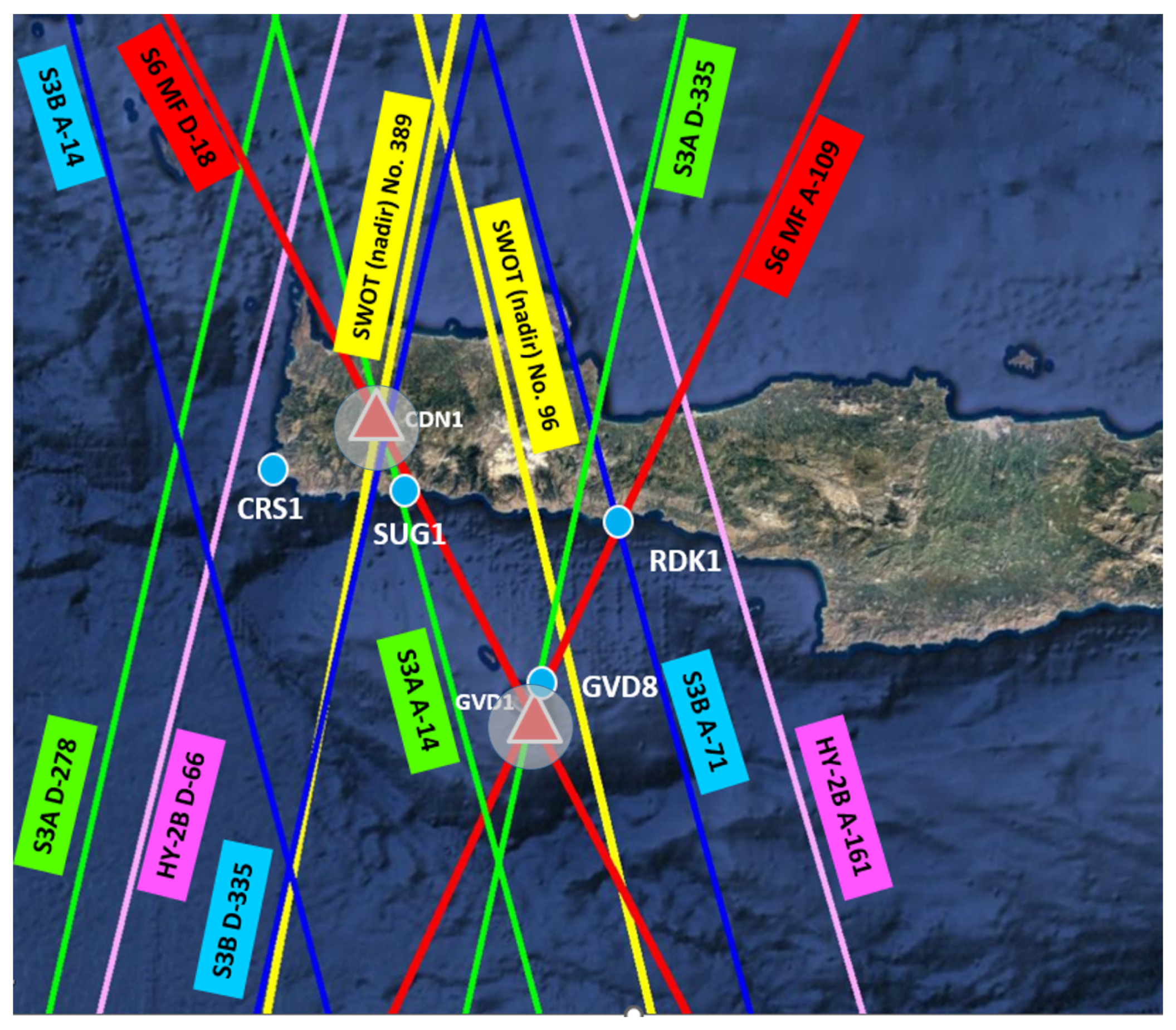
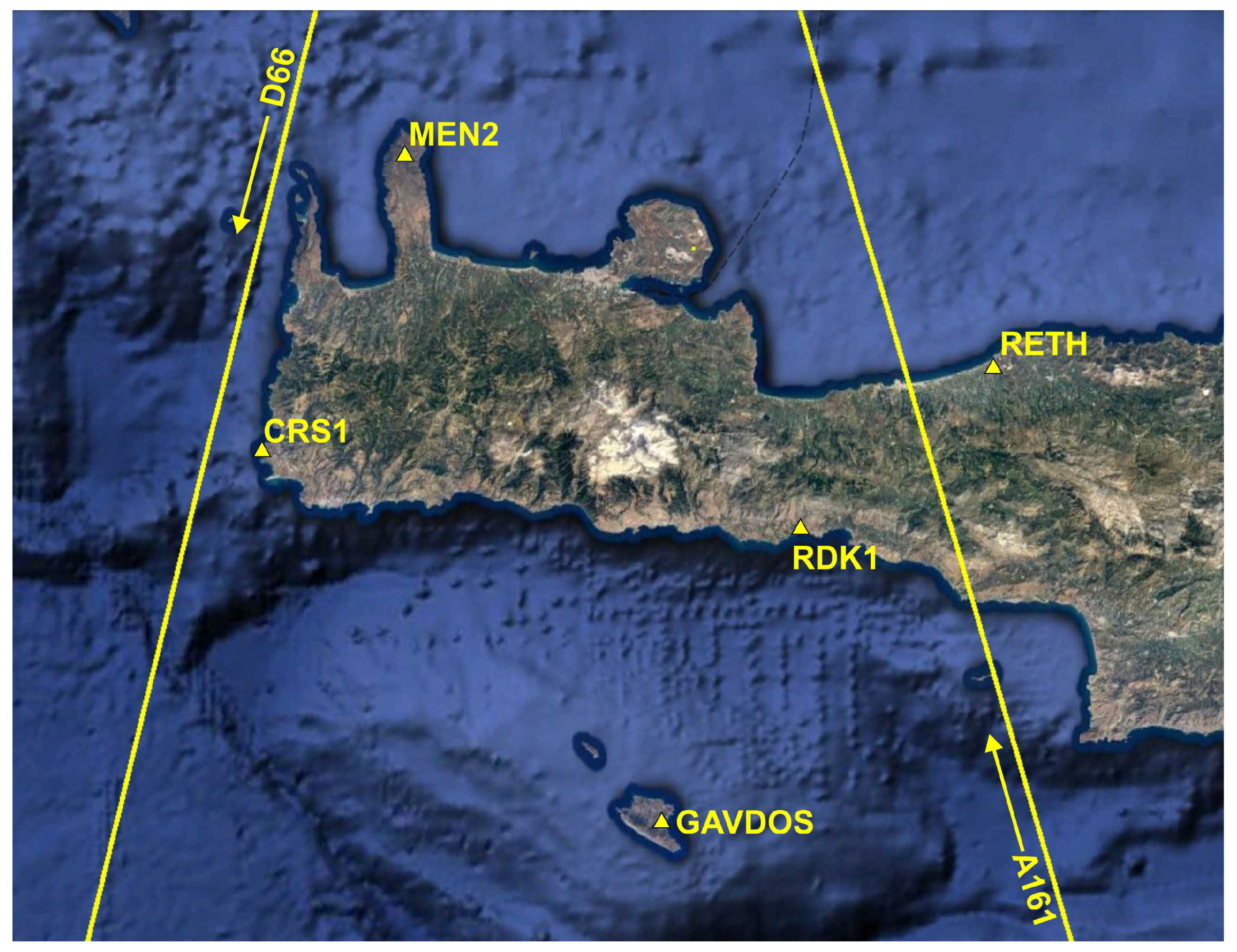
The GDR data used for this HY-2B Cal/Val correspond to cycles 17–97 and cover the period from January 2019 to July 2022. These data are organized into files. Each file represents a short arc (ascending or descending) of half a revolution and is associated with a pass number. Because of this satellite inclination, all ascending passes start at a latitude of about $\phi =-80.7^{\circ }$ and end at about $\phi =80.7^{\circ }$. The opposite start/end latitude values occur for descending passes. 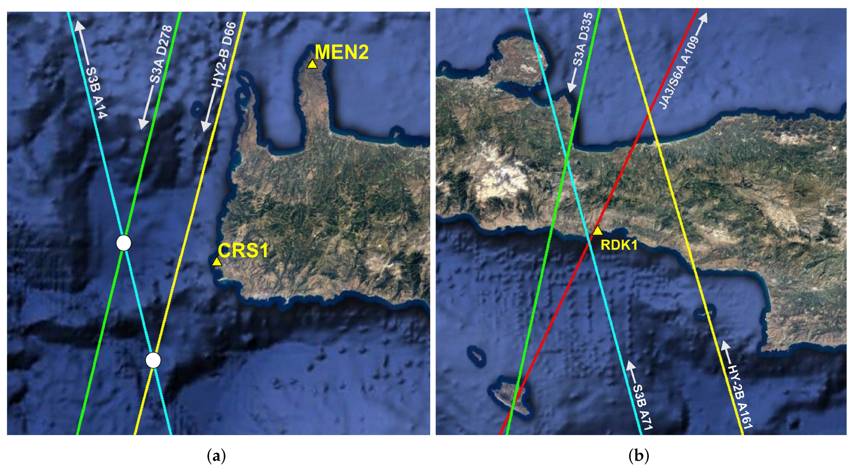The HY-2B ground track coverage in the vicinity of Crete is already presented in Figure 1 and consists of four passes. Two of these passes have been used for Cal/Val, i.e., the ascending pass A161 and the descending pass D66 (Figure 2).

In a joint effort between TUC and NSOAS to improve the HY-2B data, a careful initial quality assessment of the original release of HY-2B GDR products is regularly conducted. Several inconsistencies have been identified and resolved regarding the comparative behavior of 1 Hz and 20 Hz parameters (e.g., Ku-band range), the implementation of standard non-geophysical corrections (e.g., net instrument correction) and the availability of geophysical corrections for all measurements. This preliminary assessment resulted in a more accurate release of HY-2B data (GDR version 2).

4.2. FRM Uncertainty for Sea-Surface Cal/Val Bias

Altimetry calibration requires ground reference measurements made by tide-gauges, GNSS receivers, atmospheric sensors, oceanographic sensors, electronic monitoring devices, clocks, etc. The final Cal/Val result thus contains contributions from each element used to establish the absolute sea-surface altimetry calibration. Each one of these instruments and constituents contributes to the establishment of the results for the altimeter bias first by its own reference measurements and secondly it stipulates the definitive error budget because each one comes along with uncertainty arising from its own measurements.

In the FRM strategy, the uncertainty budget of each individual constituent in the Cal/Val process should itself be metrologically traceable. Moreover, the effort involved in establishing the metrological traceability for each constituent in altimetry calibration should be commensurate with its relative contribution to the final result.

To evaluate the uncertainty for the SI-traceable (SI: International System of Units) measurements in the altimeter calibration, we usually have no means to revert to the absolute reference for the SI units (i.e., the speed of light is the defined unquestionable parameter) for establishing all subsequent measurements and their accuracy. At first, we have to rely on a collection of information for the calibrating instruments at the Cal/Val site, such as (1) previous measurement data, (2) experience with or general knowledge of the behavior and properties of the relevant instruments, (3) manufacturer’s specifications, (4) previous calibration or other certificates, and (5) uncertainties assigned to reference data taken from external sources, handbooks, etc.

Evaluation of the uncertainty is carried out either using a Type A standard uncertainty, or a Type B standard uncertainty following the “Guide to the expression of uncertainty in measurement” issued by the Joint Committee for Guides in Metrology of the Bureau International des Poids et Measures (BIPM) [34]. Type A standard uncertainty is determined from the frequency distribution and the statistical evaluation of real observations, while the Type B standard uncertainty is derived from an assumed probability function (subjective probability) depending upon scientific judgement and the degree of belief that an event will occur (i.e., previous observations, experience, manufacturer’s specifications, laboratory calibrations, reference data, etc.). Both approaches employ the recognized interpretations of uncertainty realizations [34].

In the sequel, we will conduct a statistical investigation of every conceivable cause of uncertainty, for example, by using different makes and kinds of instruments, diverse methods of measurement, various measuring procedures, and differing approximations and environmental conditions. The uncertainties associated with all of these contributions to the calibration could be evaluated by a statistical investigation of a series of observations, and the uncertainty of each cause could be characterized by its measure of location (mean, median, etc.) and its measure of scale (i.e., standard deviation, range, biweight, etc.).

The characterization of the ground reference involves determining, for each instrument on the ground used for the satellite calibration, every component and its sub-system, and evaluating their responses to various operating and environmental conditions and settings.

Field sensor characteristics may include measurement stability, linearity, accuracy, spectral characteristics, operating conditions, etc. According to this, we evaluated the presently installed field instrumentation at the Gavdos and West Crete facilities and at the Wanshan islands. Thus, we gained confidence in building the sensor and instrument characteristics, as well as proposed different measures for the location parameters (mean value for the sought parameter) and for the scale parameters (accuracy and precision), using conventional and robust statistical estimates. Influencing parameters on the sensor and parameter responsivity may be monitored through modeling.

For the satellite altimeter calibration using sea-level procedures, several elements contribute to the final bias results. These are, although not exhaustive: (1) Absolute coordinates of the reference Cal/Val site, (2) water level, (3) control ties and ground monitoring, (4) geoid model, (5) MDT (Mean Dynamic Topography) model, (6) geophysical parameters, (7) atmospheric delays and (8) unaccounted effects.

The first step towards the determination of the FRM uncertainty of the sea-surface Cal/Val site, such as CRS1 and RDK1, is the identification of the uncertainty constituents. These may be grouped as follows:

• Tide gauge instrument: Uncertainties arising from the tide-gauge zero reference, sensor type, model and measuring principles, tide gauge vertical alignment, etc.;
• Absolute Positioning: Uncertainty may emerge from the determination of the absolute geodetic coordinates above the reference ellipsoid, the ties between GNSS and tide gauge reference points, the atmospheric delay determinations, etc;
• Reference surfaces: The reference surfaces used to transfer the SSH as measured at the sea-surface Cal/Val site location to areas with valid satellite measurements. These are: geoid, mean sea surface and mean dynamic topography, and they all come with an uncertainty;
• Processing: Integration of SSH measurements as measured by different tide gauges, transfer of sea-surface heights, processing integration, etc.;
• Unaccounted effects: Estimation of the total contribution of unidentified uncertainty constituents.

All of these have been described in detail in [13,32], but here we concentrate upon the most influential constituents of uncertainty and provide a more detailed description on the way their uncertainties are estimated specifically for the CRS1 and RDK1 Cal/Val sites.

4.3. Tide Gauge Uncertainties

4.3.1. Sensor

A nominal uncertainty, as determined under specific environmental conditions, is provided for each tide gauge by its manufacturer. However, these conditions are rarely met in practice. Thus, the measurement uncertainty of the tide gauge shall also be estimated in the field under real-life environmental conditions.

Pre-processing of tide gauge records includes screening with the removal of outliers and correction of data logger errors (e.g., removal of duplicate entries). Tide gauge observations also need to be filtered so that most of their noise is reduced while the geophysical signals are still retained. The sensors SVR1 and SVR2 of the CRS1 Cal/Val site and the RDN1 and RDN2 sensors of the other RDK1 site provide continuous measurements of the instantaneous sea level with sporadic interruptions, in case of, for example, equipment maintenance. Additional information regarding these sensors is provided in

Table 2. Tide gauge characteristics and estimated parameters.

Attributes	SVR1	SVR2	RDN1	RDN2
Sensor type	Pressure	Radar	Radar	Radar
Installation date	4/2012	8/2012	10/2009	7/2019
Sampling period	6 min	6 min	3 min	6 min
Estimated noise level	15 mm	8 mm	17 mm	12 mm
Filter cut-off frequency	15 Hz	10 Hz	19 Hz	7 Hz

.

A spectral analysis was performed to determine suitable filtering parameters that satisfy these two criteria (noise reduction, signal protection). The procedure implemented is described in the sequel, focusing on the SVR2 sensor. Similar steps were followed for the rest of the tide gauge sensors.

First, the Fourier transform $\mathcal{F}\left\{y\right(t\left)\right\}$ is used to decompose the tide gauge time series $y\left(t\right)$ into its main harmonic constituents, and to calculate its power spectral density (PSD) [35]:

$$S_y\left(f\right)=\frac{{2\left|\mathcal{F}\left\{y\right\}\right|}^2}{f_s{N}^2},$$

(1)

where $f_s$ denotes the sampling frequency of the discrete sequence, $y\left(t\right)$ (given by the reciprocal sampling period of the tide gauge sensor), and N is the number of samples in the time series $y\left(t\right)$. The resulting PSD for the SVR2 time series is given in Figure 7a, where an almost flat behavior is evident after 10 Hz. A flat PSD function implies that all frequencies contribute equal signal power and is the characteristic spectral signature of white noise. The theoretical PSD of a discrete-time white noise process $n\sim \mathcal{N}(0,{\sigma }^2)$ with a sampling period of $\mathsf{\Delta }t$ is given by [36]:

$$S_n=S\left(f_n\right)=2{\sigma }^2\mathsf{\Delta }t.$$

(2)

The standard deviation $\sigma$ denoting the uncertainty level of the tide gauge sensor can be estimated based on Equation (2) and after the power level $S_y\left(f\right)$ becomes flat. For the SVR2 sensor, $\sigma$ is estimated to be about $\pm 9$ mm, which is in good agreement with its technical specifications.

For a sampling period of $\mathsf{\Delta }t=$ 6 min, the theoretical level of the SVR2 noise PSD is marked with a bold dotted (horizontal) line in Figure 7a and is equal to $S_n=S\left(f_n\right)\approx 7\times {10}^{-7}$ m²Hz⁻¹. The PSD of a simulated white noise time series with the same stochastic properties as the estimated SVR2 noise is also given in Figure 7a. It is evident that the simulated noise and these tide gauge PSDs are in good agreement (in terms of power level) after 10 Hz. Therefore, a simple approach to suppress the white noise of these data is to use a low-pass filter with a cut-off frequency of $f_c=10$ Hz.

To ensure that geophysical signals (e.g., high-frequency ocean tides) are not significantly suppressed because of filtering, the amplitude and phase of 149 tidal harmonic constituents has been estimated by the least-squares spectral analysis [37,38]. The tidal frequencies are taken from [39] (Table A.1) and are marked in Figure 7b with vertical orange lines that span from a period of 1 year ($\sim 2.3\times {10}^{-3}$ Hz) to 2 hours ($\sim 11.73$ Hz).

A time series is synthesized from the estimated amplitudes and phases, and its PSD is also provided in Figure 7b. The power of all tidal constituents with frequencies greater than 10 Hz is close to the noise level, hence their signal contribution to the tide gauge measurements is indistinguishable from noise. The selection of a cut-off frequency of 10 Hz is therefore not expected to remove strong geophysical signatures. The filter selected to de-noise the tide gauge measurements is an FIR (Finite Impulse Response) filter of order 2001 with a Hamming window. Since the filtering requires equally-spaced data, time gaps in the tide gauge time series are filled in prior to filtering with interpolated values.

The Power Spectral Density of the filtered signal is given in Figure 7c. Finally, the comparison of the original and filtered tide gauge measurements in the time domain is presented in Figure 7d for a three-day observation window. The same analysis is also performed for the filtering of SVR1, RDN1 and RDN2 time series at the respective tide gauges. Their estimated noise level and filter cut-off frequency are shown in Table 2.

Thus, the uncertainty constituent for the observations made by each tide gauge was estimated.

4.3.2. Water Level Sampling

Although tide gauges are operating continuously, only measurements during the day of the satellite overpass are used to derive the sea-surface height at the time of the satellite overfly. Thus, an uncertainty is introduced because an estimation is required at the exact time of the satellite pass based on the applied sampling rate of each sensor (e.g., 6 min, 8 min, etc.) and the available observations.

In the sea-surface calibration, repeatability stands for the number of measurements that each tide gauge makes within the useful time period for each satellite overpass. The estimation of the uncertainty is based on the sampling rate of each master tide gauge at the Cal/Val site. For example, the SVR2 and RDN2 sensors are, respectively, used as the reference tide gauges at the CRS1 and RDK1 Cal/Val sites. Both tide gauges record the water level every 6 min. Thus, there are $N=10$ observations during the 1-hour period used for sea-surface calibration. Then, the experimental standard uncertainty (Type A evaluation) for the mean value of the water level measurements at the time of the satellite pass, as the water level remains unchanged, could be estimated:

$$u_{1,1}=\frac{s}{\sqrt{N}}=\frac{\pm 8\mathrm{mm}}{\sqrt{10}}=\pm 2.5\mathrm{mm}.$$

(3)

4.3.3. Point of Zero-Reference for Tidal Observations

The zero-reference measuring point of certain tide gauges was observed to change over time, although manufacturers may have supplied a constant value. In order to accurately calculate the offset between the tide gauge leveling point (physical sensor reference point) and its actual measuring point (phase center) a field characterization procedure is periodically implemented at the PFAC.

This procedure involves a comparison of the operating tide gauge against the tide pole readings in the field. Tide pole observations are assumed to be the most accurate technique (±1 mm) for measuring the instantaneous sea-surface height. There are three main problems in tide pole observations and sampling values in the field:

• They shall be made by an experienced observer every few minutes for a predefined period of time (i.e., 12 h). This is not always feasible in remote locations, such as the Gavdos and the Wanshan Cal/Val facility;
• Tide poles provide instantaneous estimates of the sea level, whereas, for example, a radar tide gauge repeats observations typically every 20 s (maximum: 58 s). Thus, there is a discrepancy in terms of simultaneity for the water level, as the sea water is never calm.
• With a tide pole, we measure a single point at the sea-surface, whereas radar measurements cover a wider area on the sea surface, pending its effective field of view and the sensor’s distance to the sea-surface. Thus, an averaging of a larger area of sea water is involved in tide gauge observations.

To cope with these problems, the comparison of the hourly or monthly values of tide pole observations with digital tide-gauge measurements may be carried out [32,33]. The observer may take one tide pole reading every 5 s for a 2 min interval centered on the hour. By averaging these 24 tide pole values, the hourly tide pole reading is defined. If this procedure is repeated over a 12-h period once a month, then the average of these 12 hourly tide pole readings are assigned as “monthly” values and compared against the operating tide gauge monthly values.

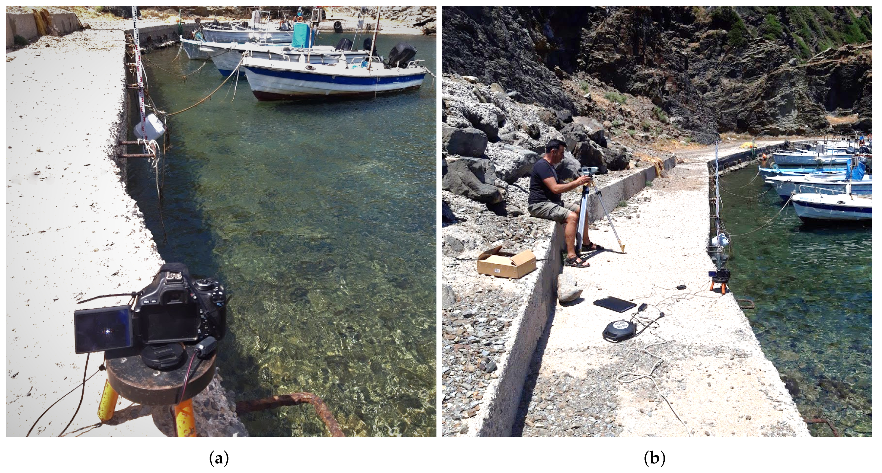
Another technique for field characterization of the operating tide gauges was devised by the PFAC team [32,33]. Instead of reading the tide pole manually, high-quality images of the tide pole are being captured by a digital camera. A digital camera is placed in front of a tide pole anchored at the Cal/Val sites (Figure 8). Water level observations, as recorded by a tide gauge, are compared against the “true” water level, as captured by the camera. A digital camera captures images, for example, at a rate of 1 min.

The experimental standard uncertainty (Type A evaluation) of a zero-reference could thus be established as:

$$u_{1,2}=\frac{s}{\sqrt{N}}.$$

(4)

where N is the number of observations made during the experiment and s is the standard deviation of observations. Details about the other remaining constituents of uncertainty have been given elsewhere [32,33].

4.4. Absolute Positioning Uncertainties

4.4.1. GNSS Receiver

The post-processing of raw RINEX data is routinely carried out for all permanent GNSS stations within the PFAC network. The main product of those post-processing campaigns is a set of estimated coordinates and velocities for each station, along with their corresponding uncertainties. Since these products are derived using well-established techniques, this subsection is focused on the analysis of the FRM uncertainty regarding the absolute positioning.

An uncertainty of $s=\pm$6 mm for the vertical component of the GNSS coordinates has, for example, been provided by the CRS1 GNSS receiver manufacturer (Type B evaluation of uncertainty). This is true provided the following specifications are met: static positioning, choke ring antenna, long geodetic baselines and long observation time. These specifications are fulfilled for the CRS1 permanent GNSS station. The manufacturer states that the uncertainty should not exceed the bounds of $s=\pm$6 mm. Assuming that it is equally probable that a new value of the uncertainty in the height coordinate lies within the interval of $-6$ mm and $+6$ mm, a uniform distribution is considered. Thus, the associated uncertainty of the expected value (mean) for the height because of this GNSS receiver could be reported as:

$$u_1=\frac{s}{\sqrt{3}}\approx \pm 3.5\mathrm{mm}.$$

(5)

The $\sqrt{3}$ in the denominator is inserted because of the uniform distribution.

4.4.2. GNSS Height Repeatability

The height of the GNSS antenna at the CRS1 site produces an uncertainty that is related to the coordinate repeatability. The time span of the GNSS data is particularly important for the accurate determination of the ellipsoidal height, as longer observation periods minimize the errors induced by satellite geometry, atmospheric delays, etc. Assuming normally distributed residuals, no autocorrelation, etc., the uncertainty for the mean value of the derived heights via GNSS processing could, for example, be expressed as:

$$u_2=\frac{s}{\sqrt{N}}=\frac{\pm 6\mathrm{mm}}{\sqrt{4769}}\approx \pm 0.09\mathrm{mm},$$

(6)

where N is the number of observations in the current time-series (i.e., days of operation) and s is the standard deviation (scale estimation).

4.4.3. GNSS Antenna Reference Point

The absolute phase center and variations of the GNSS antennas are related to the uncertainty of the height determination as carried out in the GNSS processing. Ideally, to obtain a realistic estimation for the variations of the antenna phase center, each GNSS antenna should be individually calibrated using either robot or anechoic chamber techniques [40]. When this is not possible for technical and/or financial reasons, then the GNSS antenna phase center and variations are usually retrieved by the “igs14.atx” antenna file provided by the International GNSS Service (https://igs.org/wg/antenna, accessed on 2 January 2023). This file compiles a consistent set of corrections for the offset and phase center variations of the GNSS receiver antennas, as determined by individual antenna calibrations.

Take for example, the Leica AT504 GNSS antenna operating at the CRS1 Cal/Val site. This is a relatively old antenna model which has not been previously calibrated. According to [41], a 4 mm offset in the height component of the Leica AT504 GNSS antenna was observed depending upon the method (i.e., robot or anechoic chamber) used to estimate the antenna phase center offsets.

Other studies [13,42] report that the robot and chamber-derived phase center corrections may induce position differences in the up component (height) of the order of 7 mm. Thus, the standard uncertainty at the 67% confidence level for the determination of the reference point of the certain GNSS antenna is given as (Type B uncertainty evaluation and uniform distribution assumed):

$$u_3=\frac{\pm 7\mathrm{mm}}{\sqrt{3}}\approx \pm 4.04\mathrm{mm}.$$

(7)

Again, the $\sqrt{3}$ in the denominator is inserted because a uniform distribution was assumed [34,43].

4.4.4. Processing for Coordinate Determination

The processing of the GNSS observations derived from continuously operating GNSS stations requires the calculation of daily coordinate solutions in a defined reference frame. A subsequent time series analysis is carried out to determine the station position at a reference epoch along with the station velocity in the local geodetic reference system (or North-East-Up reference system) [44]. These tasks were performed using the following software packages which employ diverse processing techniques:

• Relative differential positioning using GAMIT [45];
• Precise Point Positioning using Gipsy-X [46];
• Precise Point Positioning with Ambiguity Resolution using the Canadian positioning software (CSRS-PPP-AR), provided by the Natural Resources Canada [47,48].

The positioning and velocity results for the CRS1 permanent GNSS station are provided in

Table 3. Absolute positioning and velocity results for the CRS1 permanent GNSS station, as derived by different techniques: RD: Relative Differential; PPP: Precise Point Positioning; PPR-AR: Precise Point Positioning with ambiguity resolution (Reference epoch: 2013.5, Reference frame: ITRF2014).

Technique	$\mathit{\phi }$	$\mathit{\lambda }$	h	$\mathit{\sigma }\left(\mathit{\phi }\right)$	$\mathit{\sigma }\left(\mathit{\lambda }\right)$	$\mathit{\sigma }\left(\mathit{h}\right)$
	[deg]	[deg]	[m]	[mm]	[mm]	[mm]
RD	35${}^{\circ }{18}^{\prime }12.{649}^{″}$	23${}^{\circ }{31}^{\prime }17.{264}^{″}$	21.2075	2.029	1.924	5.716
PPP	35${}^{\circ }{18}^{\prime }12.{649}^{″}$	23${}^{\circ }{31}^{\prime }17.{264}^{″}$	21.2001	1.743	2.002	5.822
PPP-AR	35${}^{\circ }{18}^{\prime }12.{649}^{″}$	23${}^{\circ }{31}^{\prime }17.{264}^{″}$	21.2010	1.655	1.662	5.443
	$v_{\mathrm{N}}$	$v_{\mathrm{E}}$	$v_{\mathrm{U}}$	$\sigma \left(v_{\mathrm{N}}\right)$	$\sigma \left(v_{\mathrm{E}}\right)$	$\sigma \left(v_{\mathrm{U}}\right)$
	[mm/yr]	[mm/yr]	[mm/yr]	[mm/yr]	[mm/yr]	[mm/yr]
RD	−12.16	6.82	−0.93	0.12	0.10	0.28
PPP	−11.84	7.13	−0.43	0.28	0.32	0.38
PPP-AR	−11.76	7.66	−0.03	0.24	0.20	0.74

. Thus, another uncertainty arises in the applied processing technique used to determine the daily time series of the GNSS station coordinates. For Cal/Val activities, the results were derived by the relative differential positioning.

Sea-surface calibration (details provided in Section 4.1) requires the ellipsoidal height of the tide gauges. After 4769 days of GNSS operation, the standard uncertainty (i.e., 68%) for the CRS1, for example, the final ellipsoidal height, $\sigma \left(h\right)$, and its velocity per year is (see, for example, the Relative Differential results, Table 3):

$$u_4=\frac{\pm 5.716\mathrm{mm}}{\sqrt{4769}}\approx \pm 0.08\mathrm{mm}$$

(8)

and

$$u_5=\frac{\pm 0.28}{\sqrt{4769}}\frac{\mathrm{mm}}{\mathrm{yr}}\times 7\mathrm{yr}=\pm 0.02\mathrm{mm},$$

(9)

respectively. The uncertainty due to the station velocity provided in Equation (9) is estimated based on the time difference between the ellipsoidal height reference epoch (2013.5) and the HY-2B data mean reference epoch (∼2020.5), which corresponds to ∼7 years.

4.4.5. Integration of Different Processing

Integration of the three solutions and the derivation of the final coordinates for the Cal/Val site also has an uncertainty that needs to be taken into consideration. It can be observed, for example, from Table 3, that there is a difference of about 6 mm in the CRS1 height determination between GAMIT and the rest of the processing techniques, whereas the rest of the coordinates and uncertainties show sub-millimeter differences.

Thus, the ellipsoidal height uncertainty due to the processing technique coincides with the ellipsoidal height difference, as determined by the relative differential and the precise point positioning techniques, (uniform distribution assumed), i.e.,

$$u_6=\frac{\pm 6.50\mathrm{mm}}{\sqrt{3}}\approx \pm 3.75\mathrm{mm}.$$

(10)

4.4.6. Control Ties and Geodetic Surveys

Spirit leveling surveys are carried out on a semi-annual basis (minimum) to monitor any subsidence changes at the Cal/Val site. During each survey, the height difference between the GNSS antenna reference point and benchmarks established on stable ground (solid bedrock) in the vicinity are used to tie the GNSS with the tide gauge reference points.

Leveling surveys are carried out by experienced personnel and using high grade leveling equipment. The uncertainty in every individual levelling reading is $\pm 5$ mm but the uncertainty in the height difference is determined to be $\pm 0.5$ mm. Thus, the uncertainty for this group of constituents could be established as:

$$u_7=\frac{\pm 0.50\mathrm{mm}}{\sqrt{27}}=\pm 0.10\mathrm{mm}.$$

(11)

where $N=27$ is the number of surveys. Note that the CRS1 and RDK1 GNSS stations were installed in Mar 2008 and Mar 2009, respectively. Given that these leveling surveys are repeated every six months, the total number is $N=29$ for the CRS1, and $N=27$ for the RDK1 Cal/Val sites.

4.5. Reference Surfaces

The estimation of uncertainty of the reference surfaces (i.e., Mean Sea Surface (MSS), Mean Dynamic Topography (MDT), and geoid) used to transfer the sea-surface height from the Cal/Val site to the open sea, where valid satellite measurements exist, is a complicated task. In the PFAC, local models were developed in the past [49] and were verified by boat campaigns. Furthermore, global models for the MSS and the MDT were also incorporated in the sea-surface processing.

In general, the accuracy of the global/regional MDT and the MSS models is degraded as we come closer to the coast. The opposite is true for precise geoid models, as these are primarily constructed using terrestrial gravity measurements.

The regional geoid model was developed based on marine, aerial and terrestrial gravity measurements. Its uncertainty was estimated from previous investigations to be $\pm 80$ mm. Moreover, the standard uncertainty of the applied MDT model in the areas of consideration is of the order of $\pm 44$ mm. Thus, if the MDT and the geoid models, for example for the CRS1 site, are used, then the total uncertainty budget involved in these reference surfaces could be estimated as:

$$u_8=\pm \sqrt{{\left(44\right)}^2+{\left(\frac{80}{\sqrt{3}}\right)}^2}\mathrm{mm}=\pm 48.06\mathrm{mm}.$$

(12)

4.6. Cal/Val Processing Uncertainties

The processing of the in situ measurements during the sea-surface calibration is subject to uncertainties related to:

(a) Final water level estimate at the Cal/Val Site. At first, the uncertainty for each tide-gauge and its measurements is determined. This is accomplished applying regression lines to a data set of about 1 h for each tide-gauge. Then, the estimated degree of departure of observation with respect to the fitted line will provide a measure of scale (precision) for the measurements of each tide-gauge. Any departures from the estimated mean value will be brought up at this stage by a cross-comparison of different tide gauges.

The final estimate for the water level at the satellite pass time is produced as a weighted measure of location (mean, median, trimmed mean, bi-weight, M-estimator, etc.) using the tide-gauges operating at the Cal/Val site. The final estimate for water level will be double-checked against the master tide-gauge, before allowing it to take part in the Cal/Val processing.

Inter-comparison of different tide-gauge measurements is regularly carried out to monitor potential drifts, but also to gain a better knowledge of the ocean dynamics. The mean difference of the hourly values of different tide-gauges during the HY-2B overpass has been determined to be less than 10 mm and its standard deviation $\pm 12$ mm. Thus, it is safe to claim that the overall uncertainty in reporting a final water level value by combining sea-surface heights of various collocated tide-gauges, is $\pm 15$ mm (Expanded uncertainty, $U=2\times u$, at 95% confidence level). Thus, the experimental standard uncertainty (u, with 68% confidence level) for the final water level estimate at the Cal/Val site, is:

$$u_9=\frac{\pm 15\mathrm{mm}}{2}=\pm 7.5\mathrm{mm}.$$

(13)

assuming normal distribution for the tide-gauge observations.

(b) Geoid Slope, Offshore Transfer: Besides the uncertainty of the reference surfaces used to transfer the SSH from the sea-surface Cal/Val site location to open sea, there is also an uncertainty associated with the way that this transfer takes place. Another factor that induces uncertainty in the sea-surface calibration is the geoid slope. This is due to the large footprint of the satellite altimeter covering different geoid slopes in the along-track and across-track direction.

This uncertainty is estimated to be no more than $\pm 10$ mm, because major bathymetric and thus geoid changes are observed in the calibrating regions. Of course, this is only an approximation (Type B uncertainty evaluation) at present that may need to be revised at a later stage. Thus, the standard uncertainty for the geoid slope and offshore transfer could be estimated under the assumption of a uniform distribution, as:

$$u_{10}=\frac{\pm 10\mathrm{mm}}{\sqrt{3}}=\pm 5.8\mathrm{mm}.$$

(14)

(c) Processing: This is the uncertainty involved in the algorithms, the processing and calculations for arriving at the Cal/Val final results. It is estimated to be $\pm 0.5$ mm. Thus, the standard uncertainty for processing could be reported as:

$$u_{11}=\frac{\pm 0.5\mathrm{mm}}{\sqrt{3}}=\pm 0.3\mathrm{mm}.$$

(15)

4.7. Unaccounted Effects

This constituent contributes to the overall uncertainty because the unknown effects might not have been taken care of in the previous description. For example, uncertainties in the tide-gauge alignment, its ground stability, thermal expansion of the support mechanism, etc., are grouped as unaccounted effects. Our general scientific judgement and experience over the previous 20 years of providing such a Cal/Val service and practice, calls for an unaccounted effect lying with equal probability (a priori uniform distribution, Type B evaluation) within the bounds of $\pm 20$ mm. Thus, the standard uncertainty corresponding to the value for unaccounted effects in the sea-surface calibration, could be reported as:

$$u_{12}=\frac{\pm 20.0\mathrm{mm}}{\sqrt{3}}=\pm 11\mathrm{mm}.$$

(16)

4.8. Combined and Overall Standard Uncertainty for Sea-Surface Cal/Val

The previous analysis quantified the individual uncertainty for each constituent, finally contributing to the overall uncertainty of the sea-surface calibration.

The final standard uncertainty (at 68% confidence level) of the reported sea-surface calibration is described in terms of a Root-Sum-Square (RMS) value using:

$$u_{SSH}(68\%)=u\left(FRM\right)=\sqrt{u_1^2+u_2^2+u_3^2+\cdots +u_{13}^2}.$$

(17)

Substituting each standard uncertainty as previously calculated and summarized in

Table 4. Uncertainty Budget Analysis for Sea-surface Calibration.

Description	CRS1	RDK1	Wanshan
Tide-gauge sensor	±4 mm	± mm	$\pm 1$ mm
Repeatability	±2.53 mm	±2.53 mm	$\pm 2.53$ mm
Zero-point reference	±2.50 mm	±2.50 mm	$\pm 2.50$ mm
GNSS receiver	±3.46 mm	±3.46 mm	$\pm 3.50$ mm
GNSS repeatability	±0.08 mm	±0.09 mm	$\pm 0.10$ mm
GNSS ARP	±4.04 mm	±4.04 mm	$\pm 5.00$ mm
GNSS solution	±0.08 mm	±0.13 mm	$\pm 0.10$ mm
GNSS velocity	±1.96 mm	±4.55 mm	$\pm 2.50$ mm
GNSS integration	±3.75 mm	±3.75 mm	$\pm 3.75$ mm
Control ties	±0.09 mm	±0.10 mm	$\pm 0.28$ mm
Reference surfaces	±42.00 mm	±47.00 mm	$\pm 50.00$ mm
Final Water level	±7.50 mm	±7.50 mm	$\pm 7.50$ mm
Geoid slope	±5.77 mm	±5.77 mm	$\pm 3.50$ mm
Processing	±0.29 mm	±0.29 mm	$\pm 0.29$ mm
Unaccounted effects	±11.55 mm	±11.55 mm	$\pm 11.55$ mm
Uncertainty budget	±45.41 mm	±50.44 mm	$\pm 52.66$ mm

, we obtain the root-sum-square (combined standard uncertainty) value for the sea-surface calibration as: $\pm 45.41$ mm at the CRS1 Cal/Val, $\pm 50.44$ mm for the RDK1 Cal/Val in Crete and $\pm 52.66$ mm for the Wanshan Cal/Val in China.

Equation (17) assumes that each constituent of uncertainty is statistically independent of each other, and the observations are not serially correlated when the type A evaluation is put into action. This is a realistic and practical assumption, as most of the identified sources of uncertainty are not related. For example, uncertainties in the reference surfaces implemented for calibration cannot be connected to control ties and geodetic surveys, or to uncertainties of absolute positioning.

Statistical dependence is a difficult subject to handle and even more difficult to quantify [50,51]. If not treated with caution, it may lead to subtle errors. To support and establish the statistical dependence, data populations have to be examined for (a) consistency, (b) responsiveness and (c) mechanism of causation for component dependence. In other words, dependence between a component x and y has to be consistent across populations and not only on a specific Cal/Val site or a particular instrument. Secondly, if a particular component x (i.e., GNSS receiver) is replaced, then a clear-cut and consistent response will be expected on y (i.e., GNSS antenna reference point uncertainty), accordingly. Thirdly, there is a difficulty in understanding what sort of mechanism brings about a specific response in the final Cal/Val and in order to settle the association.

Dependence will not be treated further in this work. All these associations of statistical dependence and serial correlation are, at present, premature to establish with confidence. Moreover, the above treatment of uncertainties is by no way exhaustive. As more information on various uncertainties is available, the above results will be kept up-to-date; thus, they are consistent with the FRM procedure actually in use.

What is expected and crucial at this stage, is that more Cal/Val sites adopt this Fiducial Reference Measurements strategy for satellite calibrations and Cal/Val operators embrace the following procedures recommended by [34] (a) clearly describe the methods to calculate the calibration results and their uncertainty from the in situ observations and other input data; (b) list all the components of uncertainties and document how they are evaluated; (c) present the steps taken to arrive at the Cal/Val result so that it is readily followed and independently, if necessary; and (d) give corrections and constants used in the Cal/Val procedures and their sources [34]. These procedures, if followed, will lead us to a realistic, pragmatic and unquestionable way to express uncertainties and results for sea level variations and climate change with satellite altimetry.

5. The Sea-Surface Cal/Val Methodology

Satellite altimetry, when used for the long-term, consistent and reliable monitoring of geophysical and climate changes, requires a calibration of the satellite products throughout its lifetime along with an inter-calibration with respect to the other different operational altimeters.

Several techniques have been developed for the absolute and relative calibration of, for example, the satellite altimeter and its microwave radiometers.

The evolution of Cal/Val techniques closely follows the technological advances in satellite measuring techniques (i.e., Delay-Doppler, swath altimetry, interferometry, etc.). The current state of the art includes developments that enable altimeter calibrations to be carried out, not only over the ocean surface, but also on land, using transponders and corner reflectors [52]. Two such Cal/Val techniques are employed in this investigation to derive the absolute and relative sea-surface bias of the HY-2B radar altimeter, i.e., the sea-surface calibration and crossover analysis.

5.1. Determination of Sea-Surface Bias

In the sea-surface calibration, heights of the sea surface observed by a satellite are compared against measurements made independently by terrestrial and marine instruments on the Earth’s surface. Ideally, the reference instrumentation on the Earth should allow an estimation of the sea-surface height at the exact locations where the satellite measures, and of course is uncontaminated by land or other effects.

Practical options which fulfill these requirements are the establishment of calibration stations in either small islands (e.g., Gavdos island in southern Crete [26], Bass Strait in Australia, Corsica, France [53], Santa Catalina Island off the coast of California, USA, Wanshan islands next to Hong Kong, China [31], etc.) or small man-made constructions, such as the Harvest Oil Platform, California, USA [54].

The calibration of a satellite altimetry product depends on the location and the available instrumentation of the Cal/Val site. For example, when small platforms and/or GNSS buoys are employed at sea directly on a satellite ground track, then it is possible to perform a straightforward comparison of the satellite SSH against the in situ SSH. In coastal Cal/Val sites, such SSH calibration is not always possible, and the calibration has to be transferred from the Cal/Val site to several km in the open ocean. This is also the case for the coastal Cal/Val sites within the PFAC network in Crete. Such a sea-surface calibration is briefly explained in the sequel.

The instantaneous altimeter SSH, denoted as $SSH\left(k\right)$, at time $t_k$ and position $({\varphi }_k,{\lambda }_k)$, is determined as the difference between the satellite height above ellipsoid $h_k$ and the reduced range ${\rho }_k$. The reduced range ${\rho }_k$ is derived after all the corrections (i.e., atmospheric, dynamic atmospheric and tidal corrections) are applied to it. Atmospheric corrections are the sum of the ionospheric, and the wet and dry tropospheric corrections. The dynamic atmospheric correction is the sum of the inverted barometer and the high-frequency correction. Finally, the tidal term is the sum of the ocean loading tides, solid earth tides and pole tides.

Apart from the dry tropospheric correction, which has by far the largest magnitude (∼2.3 m in the absolute value), the rest of the corrections do not exceed the value of one meter, varying from the order of a few millimeters to tenths of centimeters (again, in absolute value). Different methods for deriving the wet tropospheric delay correction are described in more detail in Section 6.3, as part of the investigation of the HY-2B radiometer bias.

After the calculation of $SSH\left(k\right)$, the sea-surface height bias is determined by:

$$Bias\left(k\right)=[SSH\left(k\right)-N\left(k\right)-MDT\left(k\right)]-[{SSH}_0\left(t\right)-N_0\left(t\right)-MD{T}_0\left(t\right)],$$

(18)

with $N\left(k\right)$ and $MDT\left(k\right)$ being the reference surfaces of geoidal undulations and the mean dynamic topography at the satellite footprint, and ${SSH}_0\left(t\right)$, $N_0\left(t\right)$ and $MD{T}_0\left(t\right)$ are the same parameter values at the reference Cal/Val site and at the same time t. The final bias is calculated as an average on a profile along the satellite ground track. The evaluation of the SSH bias is affected by errors in the reference surfaces of the geoid, the mean dynamic topography, in the dynamic atmospheric, tidal corrections, etc. These have to be carefully assessed to arrive at reliable values for the altimeter bias.

5.2. Bias from Crossover Analysis

Intercalibration of a satellite altimeter with respect to another altimeter is possible when their ground tracks intersect over the ocean. All possible intersections of HY-2B form a set of such crossover locations around Crete. In order to minimize the effects of unmodeled time-varying oceanic effects, the time separation of the two satellites flying over the crossover location should be short and in general should not exceed 48 h [33].

The main advantage of this technique is that it is independent of any ground reference, thus it can be performed solely by satellite products. The bias from a crossover analysis taken at a specific location at sea is given by:

$$bia{s}_{\times }\left(t\right)={SSH}_2\left(t\right)-{SSH}_1\left(t\right),$$

(19)

where t is the time of a satellite passing from the crossover location, the subscript “2” denotes the satellite to be calibrated (in this case, HY-2B) and the subscript “1” is the reference satellite. Since measurements at the exact crossover location are unlikely to occur for two satellites, Equation (19) is evaluated after estimating (e.g., via interpolation) the values ${SSH}_1\left(t\right)$ and ${SSH}_2\left(t\right)$ from the complete series ${SSH}_1\left(t\right)$ and ${SSH}_2\left(t\right)$, respectively.

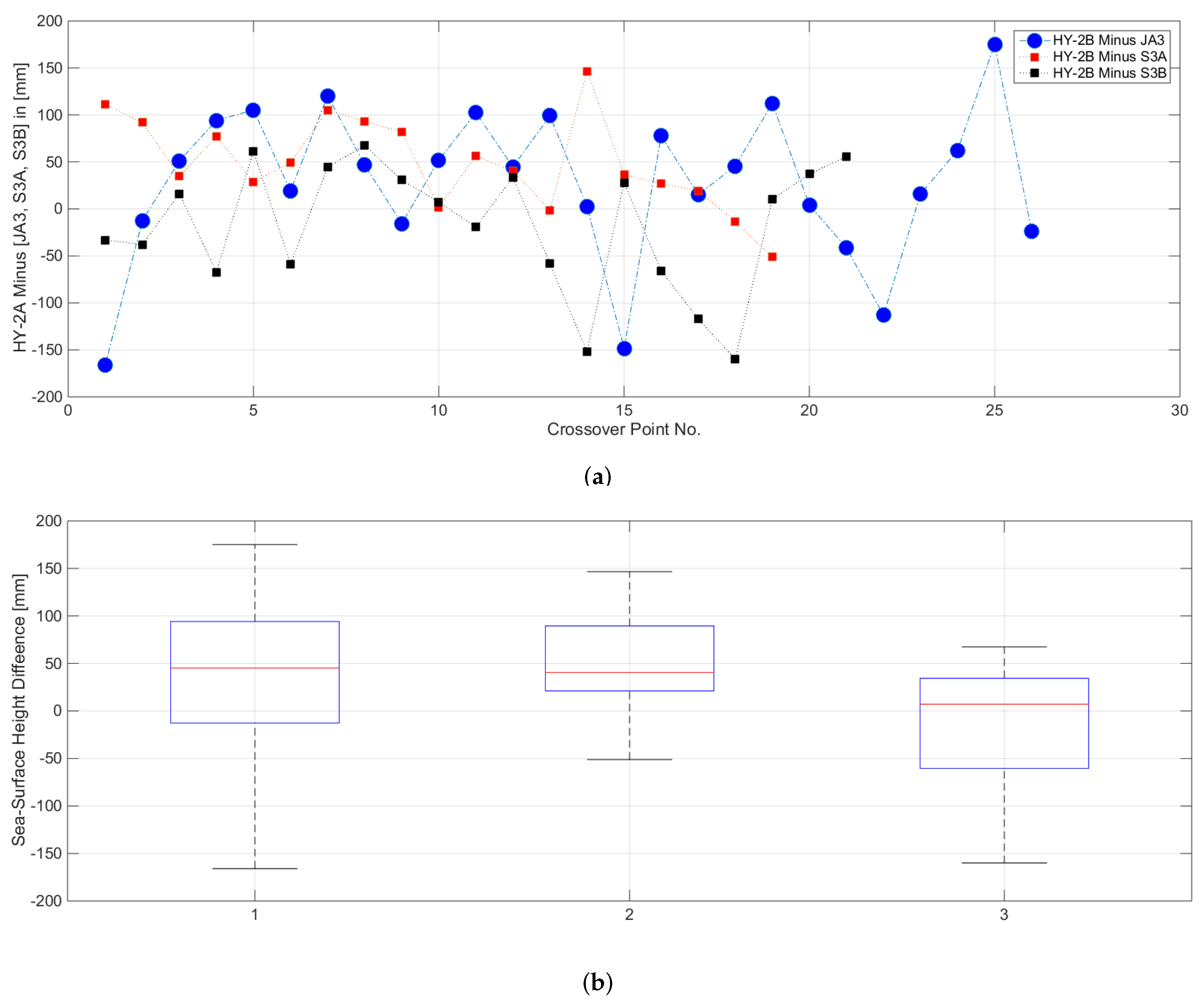
In this work, the SSH crossover bias of HY-2B with respect to Sentinel-3A/B and Jason-3 was estimated. In total, eight crossover locations were identified in the vicinity of the PFAC network around Crete (five for the descending Pass D66 and three for the ascending Pass A161). The distribution of crossover locations is provided in Figure 9.

5.3. Determination of the HY-2B Radiometer Bias

The HY-2B satellite is equipped with the scanning microwave (SMR) radiometer and with the correction microwave radiometer (CMR). Both instruments are passive sensors, but have different payloads on HY-2B. The scanning instrument is an upgraded version of the previous radiometer on-board HY-2A with improvements on the feed horns and cold sky reflector calibrations [55]. The on-board radiometer of HY-2B is used to retrieve climate parameters, such as the sea-surface temperature, sea-surface wind speed, liquid water and water vapor. The later parameter is to estimate the wet troposphere delay for reducing the altimeter range measurements.

The correction microwave radiometer is a fixed pointing microwave radiometer on HY-2B. Its function is to estimate corrections for the atmospheric wet-path delays. The CMR measures the sea-surface microwave emissivity at three separate frequencies (i.e., 23.8 GHz, 18.7 GHz and 37 GHz), the same as those implemented on the previous Jason-2 Advanced Microwave Radiometer. The 23.8 GHz channel is the primary channel for measuring water vapor. The 18.7 GHz and the 37 GHz channels, which have less sensitivity to water vapor, are used to remove the effects of wind speed and cloud cover. The beams of the CMR are co-aligned with the altimeter footprint.

Satellite altimeter observations require corrections for their measured ranges to compensate for propagation delays on the electromagnetic signal because of the atmosphere and primarily of the troposphere. These types of passive radiometers are known to operate properly over ocean, but their observations are contaminated by land when the satellite radiometer is within a distance of about 40–50 km from the coast [56].

In this work, the wet troposphere delay, as given in the GDR data of the HY-2B, is compared against GNSS-derived values (see, for example, [57]) and also against two global models provided by the National Centers for the Environmental Predictions/National Center for Atmospheric Research (NCEP) and the European Centre for Medium-Range Weather Forecasts (ECMWF).

Profiles of the corrections for the wet-troposphere delays of the HY-2B radiometer were plotted along its descending pass D66 and its ascending pass A161 and with respect to distance (actually latitude in degrees) from the CRS1 and the RDK1 Cal/Val sites, respectively. Indicative profiles are shown in Figure 10 for cycles No. 42 and 61 (D66), and cycles No. 27 and 58 (A161). Data plotted are for the HY-2B radiometer observations, the ECMWF and the NCEP models and also for the GNSS-derived corrections from (a) the two permanent sites at the CRS1 Cal/Val site, and the MEN2 station in the northwest of Crete (D66, see also Figure 11); and (b) the RDK1 Cal/Val site, and the RETH station close at the city of Rethymnon, at the north-central coast of Crete (A161).

The radiometer observations are obliviously contaminated (dramatic drops shown in Figure 10), because of satellite proximity to the landmass of Crete. Moreover, the footprint of the HY-2B radiometer changes in size between 30 and 70 km (nominal footprint size 40 km). Thus, no proper radiometer measurements are made by HY-2B in the region (+85 km north, −50 km south) around the CRS1 Cal/Val site along the pass D66. Radiometer measurements become normal again when the satellite is about 50 km away and south of the CRS1 Cal/Val site.

Presently, along the ascending pass of A161, the HY-2B satellite approaches Gavdos and the RDK1 Cal/Val sites from south going north. Radiometric observations of HY-2B are also compared, in this case, with the GNSS-derived values of the RDK1 and RETH stations and the corresponding NCEP and ECWMF models. Two of those cycles of the HY-2B radiometer profiles have been selected and shown in the bottom graphs of the Figure 10.

Figure 10c depicts a good case of the agreement with wet troposphere corrections, while Figure 10d illustrates an example of a bad disagreement of various corrections. The points of the fitted model (yellow circles) are coming from an application of a robust regression line fitted to the satellite radiometric observations. It is obvious that this fitted regression line represents a good model for the case when data are land contaminated and makes the comparison with ground stations possible. The final results for the HY-2B radiometer bias are given below in Section 6.3.

6. Results

6.1. The HY-2B Sea-Surface Height Bias

The HY-2B GDR products, as described in Section 4.1, and the methodology of Section 4.2, are used for the determination of the sea-surface height bias of the HY-2B altimeter at the CRS1 (Crete), RDK1 (Crete) and Gavdos Cal/Val sites for each orbital cycle (Figure 11).

An additional filtering of the GDR data is performed using the criteria presented in [16]. Measurements with values outside the valid intervals are considered outliers and are removed from the subsequent analysis. Measurements with ground tracks over land areas or with an altimeter footprint overlapping with land areas are also disregarded to minimize land contamination. The wet tropospheric delay correction for the Cal/Val computations is taken directly from the GDR products, which implement the NCEP model.

Figure 12 shows the sea-surface calibration results based on the CRS1 reference site. The average value of the bias is $B\left(\mathrm{D}66\right)=+9$ mm ± 5 mm, although the FRM uncertainty is $u\left(\mathrm{FRM}\right)=\pm 45$ mm (see also Table 4). It appears that there are two different sets of results: one with data up to cycle No.31 and a second set after cycle No.40. The first set seems to produce a slightly negative bias for the HY-2B, but the second set is spread around the zero bias. The gap of the no bias values between cycles No.31 and No.41 is because no data were available from the CRS1 Cal/Val site, as the station was under service.

Moreover, Figure 13 shows the sea-surface calibration results based on the RDK1 Cal/Val site and based on the ascending orbit A161 coming from the south to the central part of Crete. The average value of the bias is $B\left(\mathrm{A}161\right)=+8$ mm ± 8 mm, although the FRM uncertainty is $u\left(\mathrm{FRM}\right)=\pm 50$ mm (see also Table 4). Figure 14 shows again the Cal/Val results of HY-2B along the ascending orbit A161 using both the Gavdos and the RDK1 reference sites. Gavdos Cal/Val site gives an average bias of $B\left(\mathrm{A}161\right)=+2$ mm ± 9 mm. The observed trends of both Cal/Val results in this diagram are similar, although the Gavdos results are a bit more noisy than those of the RDK1.

Finally, Figure 15 shows the HY-2B sea-surface bias estimated using the Wanshan Cal/Val infrastructure in China. Using the facility at Zhiwan island, we estimate the sea-surface bias of HY-2B from cycle 31 to cycle 97 as $B\left(\mathrm{D}375\right)=-38$mm ± 3 mm. Previous Cal/Val results using 2–54 cycles indicate that the HY-2B bias were determined as $+4$ mm and $+12$ mm by the Qianliyan and Wanshan sites, respectively [31].

It appears that the HY-2B bias estimated at Wanshan is slightly different from that determined at the Crete sites, which were a few mm, respectively. We continue this investigation by comparing the HY-2B with other satellite altimeters.

6.2. The HY-2B Bias from Crossover Analysis

The HY-2B observations for sea-surface heights were examined with respect to the reference altimeters, such as Jason-3, Sentinel-3A and Sentinel-3B, around Crete and at sea points where satellites cross over each other. The separation time between different satellite passes is selected to be less than 2 days (48 h). The crossover points chosen for comparisons at sea are those shown in Figure 9. Differences are examined with respect to the descending HY-2B orbit D66, and its ascending orbit A161. The period covered over this analysis is from January 2019 to December 2021.

The results for the sea-surface height analysis over both ascending and descending orbits of HY-2B are as follows: [HY-2B−Jason-3] $=+33$ mm ± 18 mm ($N=11$); [HY-2B−Sentinel-3A] $=+46$ mm ± 11 mm ($N=14$); and finally [HY-2B−Sentinel-3B] = $-5$ mm ± 15 mm ($N=11$). Figure 16 shows the dispersion of these differences of sea-surface heights of HY-2B in relation to the heights from the reference altimeters at crossover points.

The Cal/Val results from this crossover analysis are based on small sample sizes ($N<20$); thus, no reliable confidence could be built on conclusions at this stage. Moreover, it has been observed that (1) Cal/Val results based on crossover points determined by different satellite ground tracks produce slightly different results even for the same satellite altimeter; (2) the satellite S3B seems to produce smaller bias at crossovers when compared with Jason-3 and S3A and in reference to HY-2B (see also boxplot diagrams of Figure 16b).

6.3. HY-2B Radiometer Bias

As described in Section 5.3, observations from the HY-2B radiometer were compared against values derived from the permanent GNSS stations at the CRS1 and MEN2 Cal/Val sites in Crete.

Table 5. Differences of wet tropospheric corrections as derived from the radiometer on-board HY-2B, CRS1 and MEN2 GNSS stations, as well as the NCEP and ECMWF global models.

Difference ($\mathit{N}=$ 67)	Average	$\mathit{\sigma }$
HY-2B AMR–CRS1(GNSS)	−7 mm	$\pm 27$ mm
HY-2B AMR–MEN2 (GNSS)	+7 mm	$\pm 30$ mm
HY-2B AMR–ECMWF	+3 mm	$\pm 24$ mm
HY-2B AMR–NCEP	−13 mm	$\pm 25$ mm

summarizes differences (i.e., average and standard deviations) of wet troposphere corrections derived from the satellite radiometer and those values from the CRS1 and MEN2 ground reference stations as well as the ECMWF and NCEP models. Average values and standard deviations, shown on the Table 5, have been estimated using sample sizes of $N=67$.

Figure 17 shows the dispersion of wet troposphere corrections, as determined by (1) the robust regression model applied on the HY-2B radiometer measurements (AMR instrument), particularly over regions where land contamination takes place, (2) computed values as determined through the ECMWF and NCEP models, and (3) the corrections derived by the GNSS observations at the stations alongside the descending pass D66, i.e., CRS1 and MEN2, as well as along the ascending pass A161 stations, i.e., RDK1 and RETH. The dspersion of corrections on Figure 17 is shown as a function of the HY-2B cycle number.

It could be observed on Figure 17d that the GNSS-derived values from the RDK1 station are a bit noisy because of the mismodeling caused by a large mass of Crete mountain over this region around the GNSS station (see also [58]). These results and comparisons along the descending and the ascending passes around western Crete reveal that the HY-2B radiometer works well and within its specifications.

7. Conclusions

In this paper, the performance of the Chinese satellite altimeter HY-2B was evaluated using two ground infrastructures: (a) the infrastructure established by the Altimetry Calibration Cooperation Plan administered by the National Ocean Application Service of China, and (b) the ESA permanent facility for altimetry calibration in Crete.

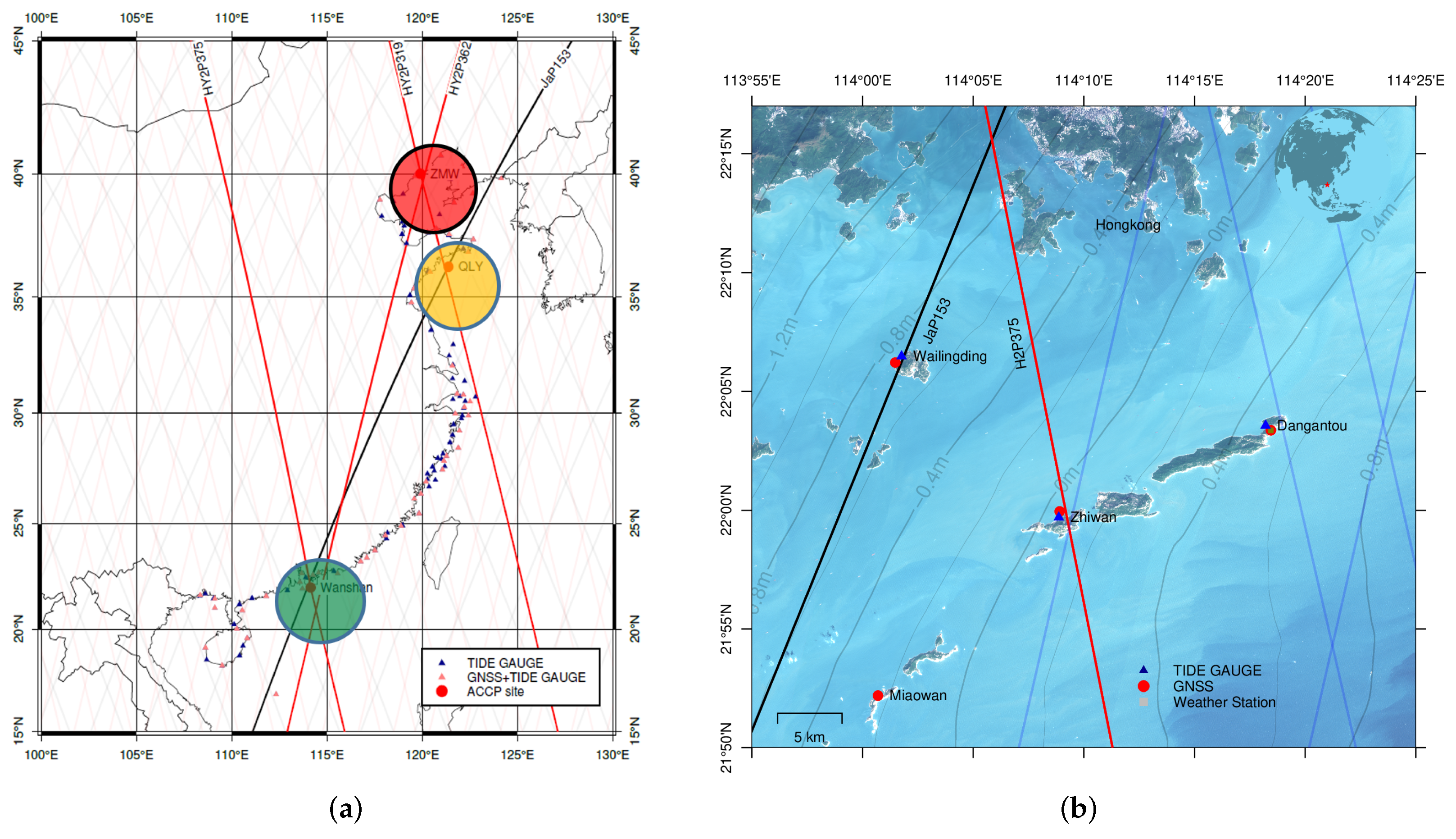
The Chinese Cal/Val infrastructure consists of facilities established on three small islands (i.e., Dangantou, Zhiwan and Wai Lingding) over the Wanshan-dedicated site, south of Hong Kong. More than 30 domestic institutes are taking part in this Cal/Val activity in China. At present, data from the Wanshan site are open to institutions in China. The second infrastructure is the permanent facility for altimetry calibration of the European Space Agency consisting of four sea-surface Cal/Val sites and two microwave transponder sites in western Crete, Greece.

In China, the Cal/Val site at Zhiwan island was used to calibrate the HY-2B altimeter along its ascending pass No. 375. The sea-surface bias over this China Cal/Val site was determined to be $B\left(\mathrm{A}375\right)=-38$ mm ± 3 mm using cycles 31 to 97 and the GDR Version C. Its FRM uncertainty budget for that result was established to be $u\left(FRM\right)=\pm 52.66$ mm. The previous Cal/Val results using 2–54 cycles indicate that the HY-2B bias was determined as $B=+4$ mm and $B=+12$ mm by the Qianliyan and Wanshan sites, respectively [31].

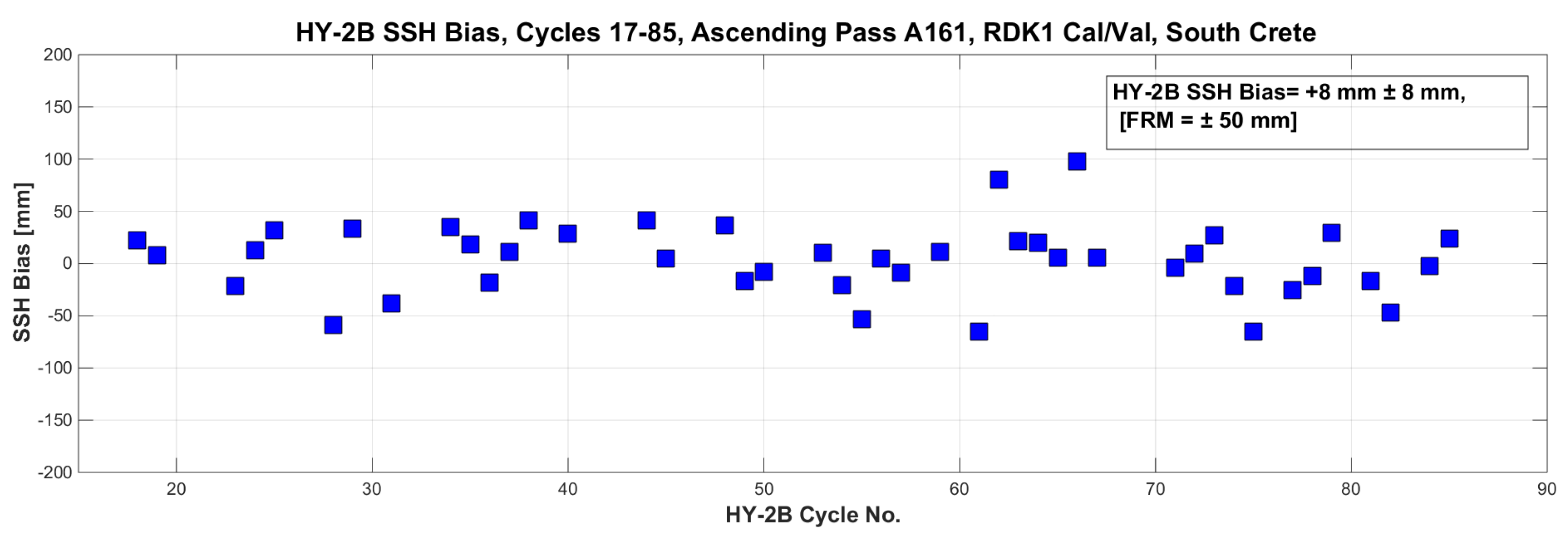
In Europe, the Cal/Val results for HY-2B were determined using the descending pass No.66 and its ascending pass No.161 and two different sea-surface Cal/Val sites in western Crete. The results were $B\left(\mathrm{D}66\right)=+9$ mm ± 5 mm using the CRS1 Cal/Val site, and $B\left(\mathrm{A}161\right)=+8$ mm ± 8 mm using the RDK1 reference site and GDR Version C. Again, the FRM uncertainty was determined $u\left(\mathrm{FRM}\right)=\pm 45$mm for CRS1 and $u\left(\mathrm{FRM}\right)=\pm 50$ mm, for the RDK1 site.

The crossover analysis of the HY-2B altimeter in reference to the Jason-3, Sentinel-3A and Sentinel-3B shows that HY-2B measures a bit higher than 1 cm, approximately, versus those reference missions, although the results need more observations to place more confidence in them.

Finally, the radiometer of the HY-2B satellite altimeter was validated using the established models of ECMWF and NCEP, as well as the respective wet troposphere values derived by the GNSS stations at permanent sites on the ground. It was demonstrated that the HY-2B Correction Scanning Radiometer observes wet troposphere delays with an uncertainty of a few mm based on the preliminary results given by the GNSS-derived wet troposphere in Crete.

In this Dragon research initiative, the HY-2B satellite altimeter was calibrated and monitored using uniform and standardized procedures, as well as protocols and best practices that were built upon trusted and indisputable reference standards at both Cal/Val infrastructures in Europe and China. A detailed analysis of the uncertainty budget for the HY-2B altimeter was presented to set it as an example for all the Cal/Val activities to follow.