1. Introduction
LiDAR point clouds are a rich source of accurate 3D information useful for various computer vision tasks. This information consists of 3D spatial, topological, contextual, and geometric relationships that are difficult for machines to process in their raw form due to their complex representation in 3D. Earlier work involved the representation of scenes in an intermediate format such as mesh, voxel or volume pixels, surfaces, etc. Using these representations as inputs for automated processing with Deep Learning needs to be sufficiently interpretable. Additionally, rendering 3D scenes with these 3D representations is challenging due to a large number of points and non-uniform point density in 3D volumes. However, there have been significant improvements in implementing 3D data processing tasks for the automated processing of LiDAR scenes.
To overcome these problems, this research proposes data-driven compressive sensing (CS), which builds on the concepts of neural reconstruction for directly processing raw 3D LiDAR point clouds based on their geometric features.
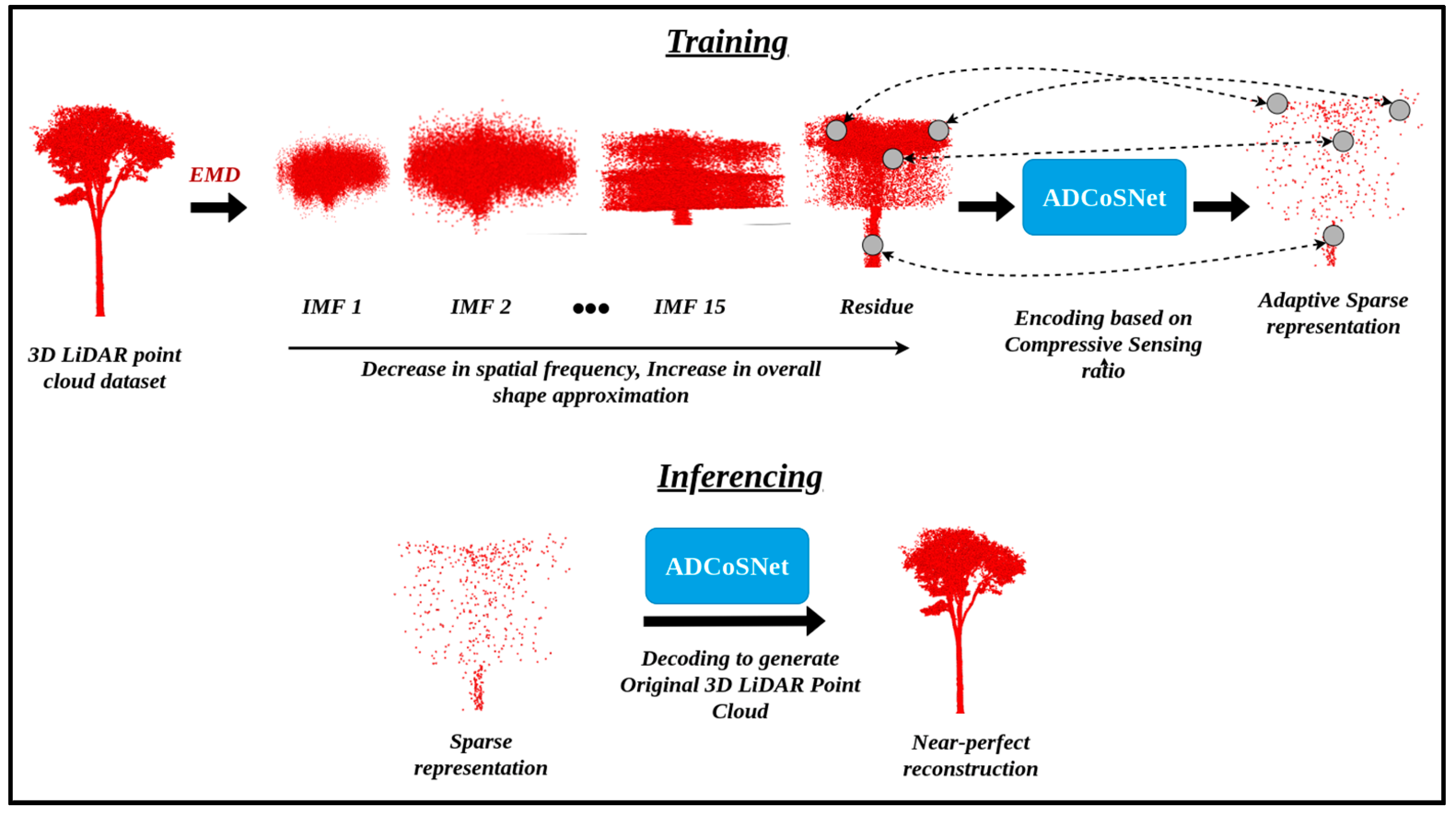
Figure 1 illustrates the overall workflow of the proposed approach, named ADCoSNet. The proposed ADCoSNet is a deep-learning-based convolutional CS framework capable of combinedly computing sparse representation from 3D LiDAR point clouds and subsequently, reconstructing the original point cloud from the sparse samples. The convolutional CS framework of the proposed ADCoSNet is based on Empirical Mode Decomposition, an adaptive decomposition algorithm as a data-driven transformation basis, as opposed to structured transformation bases such as Fourier, wavelet, etc. EMD is a widely used signal-processing technique for separating components based on spatial frequency. The proposed ADCoSNet follows the physics-informed deep learning paradigm and is a deep neural network for generating adaptive sparse representations of the 3D LiDAR scenes. The proposed approach is a novel attempt to fuse the data-driven transformation basis for adaptive representation in a convolutional compressive sensing framework for 3D forest reconstruction.
1.1. Background and Motivation
Compressive Sensing (CS) theory allows the near-perfect reconstruction of 3D LiDAR point clouds from a small set of sparse measurements, also termed sparse recovery. Conventionally, Compressive Sensing implementation is iterative in nature, and implementing it for big 3D LiDAR point clouds is challenging. To overcome this, deep network based convolutional CS is implemented. The proposed ADCoSNet builds on this principle for reconstructing 3D LiDAR point clouds as LiDAR point sets show inherent sparsity due to redundancy in storage and high spatial resolution (in cms).
By design, CS implementation utilizes structured functions for sampling the points leading to a data-agnostic implementation. The addition of a data-driven transform in the CS implementation brings adaptivity to the 3D reconstruction. This is of prime significance for 3D reconstruction of homogeneous environments such as forests.
Compressive Sensing is advantageous in less memory requirements, high data transmission rate, and fewer energy requirements for processing. Forest LiDAR scans require a huge scanning time which is usually followed by pre-processing for further applications. Adaptive Compressive Sensing addresses both the issues of—(1) high scan time by enabling faster and more efficient acquisition followed by reconstruction and further (2) supporting data-driven reconstruction.
1.2. Empirical Mode Decomposition
The Empirical Mode Decomposition (EMD) is a powerful technique for signal analysis as it can adaptively decompose signals into components varying in spatial frequency. The spatial frequency represents the repetition per unit distance (the norm in that vector space). EMD generates a series of sparse representations according to the input signal. This is different from “structured” or “rigid” transforms such as Fourier, Wavelet transforms [
1], etc. This makes the EMD a natural choice as a data-driven transform, considering most real-world signals are nonlinear and non-stationary. Using a fixed transformation basis leads to a loss in local geometric and shape features. The authors in [
2] proposed using a constructed dictionary via Takenaka–Malmquist Functions for estimating the measurement matrix (representation function).
Generally, EMD is preferable for analyzing real-world signals because of its adaptability, data-centric design, and decomposition flexibility. In addition, it captures multi-resolution features due to its implementation. In EMD [
3,
4,
5], the transformation basis for decomposition is not pre-determined and, instead, learned empirically by modeling the input data as a combination of frequency-varying components. These components are named intrinsic mode functions (IMFs) and are derived from the sifting process.
EMD was initially designed for time-series signals but is now used to transform 1D, 2D, 3D, and multidimensional datasets by decomposing the signal components (IMFs) with varying frequencies. The derived IMFs can be used as approximations of the input data. This research proposes using the last IMF, which captures the overall geometric shape of the forest due to its homogenous structure. The homogeneity is attributed to vegetation and ground classes compared to, for instance, heterogeneous urban environments with buildings, roads, poles, etc.
This difference in reconstruction approach for different domains can be understood with the help of Digital Surface Models (DSMs). The DSM of forests is different from the DSM of an urban scene. DSM for forests is more homogenous as compared to DSM for urban scenes such as cities. This is attributed to the presence of buildings, electrical towers, etc., in a city leading to a sharp variation in the surface model, unlike forests with the majority of vegetation. Because of this, and based on the statistical tests, this research utilizes only the residue component of the empirical mode decomposition (EMD) on sparse LiDAR data for forests. The readers are recommended to refer to the seminal works in [
6,
7] for comprehensive details on the multidimensional multivariate EMD.
1.3. Empirical Mode Decomposition for 3D Geometry
In Ref. [
8], EMD and Hilbert spectra computation is proposed for 3D geometry processing by transforming 3D point clouds to the 3D surface via space-filling curves (Z-curve, Hilbert curve, Gosper curve, etc.) where the authors advocate using an effective approximate Hamiltonian cycle as a representation for the 3D surface. In a similar application domain for 3D geometry processing [
9], the authors propose a 3D surface modeling framework based on a new measure of mean curvature, computed via the inner product of the Laplacian vector and vertex normal. This measure is subsequently used as a surface signal for performing EMD. In another work [
10], targeting 3D geometry processing, EMD on surfaces is proposed where the envelope computation is based on solving bi-harmonic fields with Dirichlet boundary conditions. In [
11], the authors propose a multi-scale geometry detail reconstruction based on EMD and advocate using EMD for recovering multi-level finer details.
To implement EMD on 3D point clouds (without first transforming them into 3D surfaces) [
12], the authors propose a multi-scale mesh-free EMD by iteratively extracting the detail level from the input signal and leaving the overall shape in residue. Using the last IMF aligns with the approach advocated in [
12]. In this work, the target 3D structure for processing is 3D models. However, in our work, the target 3D structure is 3D scenes (3D LiDAR scans input LiDAR scenes of forests), introducing the challenge of involving multiple geometrical attributes and shapes. Additionally, trees in forests have complex geometry because of the crown cover at the top and the stem at the bottom. For 3D LiDAR remote sensing for forests, our work is the first attempt to use multi-dimensional EMD for decomposing 3D LiDAR scenes. The readers are recommended to follow [
13] for a comprehensive analysis of the best practices for applying EMD and derived algorithms.
1.4. Compressive Sensing
Compressive Sensing (CS) is a widely used mathematical approach for smart and efficient sampling and storage in terms of sparse representations. The CS ensures near-perfect reconstruction of raw data from a small set of measurements subject to two conditions on Sparsity and Restricted Isometry Property (RIP) [
14]. The sampling basis (
) should follow the Restricted Isometry Property (RIP), whereas the representation basis or transformation basis (
) should ensure a sparse representation. Typically, the CS is an inverse problem and requires iterative linear programming solvers to solve the optimization problem.
1.5. Deep Learning for Compressive Sensing of 3D LiDAR
Recently, Convolutional Neural Networks (CNNs) have greatly improved various machine vision tasks with structured and unstructured datasets [
15,
16,
17,
18,
19,
20,
21]. Similar to [
22,
23,
24], various deep network-based CS reconstruction algorithms for images have been proposed and implemented. The authors in [
25] propose ReconNet for reconstructing blocks of images and denoising the blocks to reconstruct the complete image. Similarly, in [
26] the sampling problem for block compressed sensing (BCS) is modeled as a distortion minimization problem and a neural network is proposed to predict the distortion model parameters. ConvCSNet [
14] trains the CNN-based CS reconstruction network using entire images instead of blocks to avoid blocking artifacts. In [
27], a saliency-based sparse representation approach is proposed for point cloud simplification based on dictionary learning. With urban remote sensing perspective [
28], a reconstruction model is proposed for reconstructing city-building 3D models from sparse LiDAR point clouds is proposed.
The deep CS reconstruction networks use a group of stacked convolutional layers for hierarchical feature extraction. Based on this [
29,
30,
31,
32], model optimization is designed as deep networks using stacked convolutional layers where the network parameters are learned. In [
33], an end-to-end network is proposed for multimedia data processing, specifically video reconstruction, which integrates measurement and reconstruction into one framework. This is possible due to the differentiable design of neural networks and the capability of translating physical models as differentiable functions. The authors in [
34] proposed Incremental Detail Reconstruction (IDR) and Measurement Residual Updating (MRU) modules as a similar concept to IMFs and Residual function for CS recovery of 2D images. In [
35], a design method is discussed utilizing the modular convolutional neural network model by connecting multiple modules in parallel. The readers are recommended to follow a comprehensive review of deep learning techniques for compressive sensing-based reconstruction and inference for a detailed understanding of the topic [
36].
In LidarCSNet [
37], we used random Gaussian distributions as sampling function (
) and convolutional features as representation function (
) for reconstructing the 3D LiDAR point clouds. It is observed that such reconstruction is non-adaptive to the data distribution. As an extension to LidarCSNet, this research combines EMD-derived IMFs and the convolutional features to form a representation basis (
), leading to adaptive CS reconstruction. Our proposed ADCoSNet is based on similar concepts and is an end-to-end learning framework for (1) generating sparse measurements followed by (2) reconstructing the original 3D LiDAR point cloud from these measurements. In this work, we select different CS measurement ratios—0.04, 0.10, 0.25, 0.50, and 0.75—for sampling and generating sparse measurements. The sparse measurements can then be used for reconstructing the 3D LiDAR scenes with near-perfect accuracy.
1.6. Empirical Mode Decomposition-Driven Compressive Sensing
Data-driven approaches in deep learning focus on systematically changing the input data to the neural model to improve performance. This work advocates incorporating the last IMF, the Residual function, as an input to the deep convolutional compressive sensing (CS) framework. All-natural signals are believed to be represented in a sparse form in their raw representation or after transforming it to a sparse subspace. Due to this, the CS framework is typically non-adaptive in its implementation. This leads to challenges in the geometric processing of shapes, where low-resolution or low-scale features are usually ignored due to the size of the convolutional filter. To address this issue in 3D geometry processing, our approach proposes using the EMD-derived residual function (last IMF) as the representation basis by augmenting the Residual function with the convolutional feature set. The sampling matrix is a random Gaussian matrix attributed to its ability to follow the RIP [
14,
38,
39] with high probabilities.
Equation (1) defines the objective function for the CS-based sparse recovery.
where
=
, st means “subject to the condition”.
Equation (1) can also be formulated as Equation (2) below:
where
represents the original point set matrix,
represents the sampling basis matrix,
represents the representation basis matrix,
is the sparse representation vector,
f is the feature set representing the convolutional stack, and
q represents the EMD-derived Residue function from the 3D LiDAR point clouds.
Equation (1) is also known as the
minimization problem and is proven to produce near-perfect reconstruction for a sparse input signal. Our proposed approach can be accurately described by Equation (2). The objective is to learn a universal approximation function based on a deep network for perfectly reconstructing
x from its sparse representation
z. We present our evaluation results on the publicly available forests LiDAR scenes provided by the OpenTopography platform [
40]. The evaluation is performed by comparing the reconstructed point cloud with the original one based on the following evaluation metrics—PSNR (Peak Signal to Noise Ratio), RMSE (Root Mean Squared Error), and Hausdorff point cloud-to-cloud distance. Based on the above discussion regarding EMD-driven convolutional CS-based adaptive 3D sparse reconstruction, the problem addressed by this research can be formulated as objectives described in the next subsection.
1.7. Problem Formulation
The proposed research focuses on addressing the following objectives:
To decompose any input point set into spatially varying intrinsic mode functions (IMFs) 1, 2, … q, where q = number of IMFs, using the adaptive decomposition algorithm—Empirical Mode Decomposition (EMD). To perform qualitative and quantitative analysis on the IMFs and residual function.
Compute sparse representation, z based on sampling matrix, —a random Gaussian matrix as a measurement matrix, as a tensor product of the last IMF (q), also known as residual function, with the convolutional features, f.
i.e., = , and = = (q f)
where x , , , z , n represents the number of points in the input point set, m represents number of sampled points, d represents the number of attributes of each point in the point set, and f is the feature set representing convolutional stack.
To validate the efficacy of the proposed approach by investigating LiDAR-derived results such as Canopy Height Model (CHM) and 2D vertical elevation profiles. Additionally, analyzing the variation in 2D vertical elevation profiles of the reconstructed LiDAR point clouds with respect to the original LiDAR point clouds.
The core contributions addressing the above-mentioned objectives are highlighted in
Section 1.8 below.
1.8. Core Contributions
Our research contribution primarily incorporates a data-driven transform in a Compressive Sensing-based sparse representation and 3D reconstruction framework. The core research contributions are elaborated below:
ADCoSNet: a novel Adaptive Decomposition-driven Compressive Sensing-based Neural Geometric Reconstruction Network capable of
- ◦
Generating adaptive (data-dependent) sparse representations from 3D LiDAR point clouds for a chosen CS measurement ratio;
- ◦
Reconstructing a near-perfect 3D LiDAR scans from sparse representations.
Investigation of EMD-derived IMFs and residual function of 3D LiDAR point clouds based on visual interpretation and statistical significance.
Analyze the effectiveness of the proposed ADCoSNet for 3D forest LiDAR point clouds in terms of reconstruction fidelity for various CS measurement ratios. Investigation of 3D reconstruction performance based on LiDAR results such as canopy height model (CHM) and 2D elevation profiles.
1.9. Challenges
Although the proposed ADCoSNet poses adaptive data-driven 3D reconstruction, it is challenging to generalize a single model across all the application domains. Additionally, being a data-dependent approach, the efficacy of the proposed approach is highly dependent on the quality of the data. However, with the increasing efforts by data curators and providers to provide high-quality data, this challenge is conveniently addressable.
The rest of the paper is structured as follows.
Section 1 presents the introduction and prior work related to our proposed work.
Section 2 formulates the problem statement, while the methodology is discussed in
Section 3.
Section 4 presents comprehensive investigations and evaluation results for the extensive experiments performed over the dataset based on selected evaluation metrics, followed by a discussion of the results.
Section 5 concludes the research henceforth acknowledging various sources that played an important role in conducting this research.
2. Materials and Methods
This section describes dataset details and acquired methodology for the proposed research.
2.1. Dataset Details
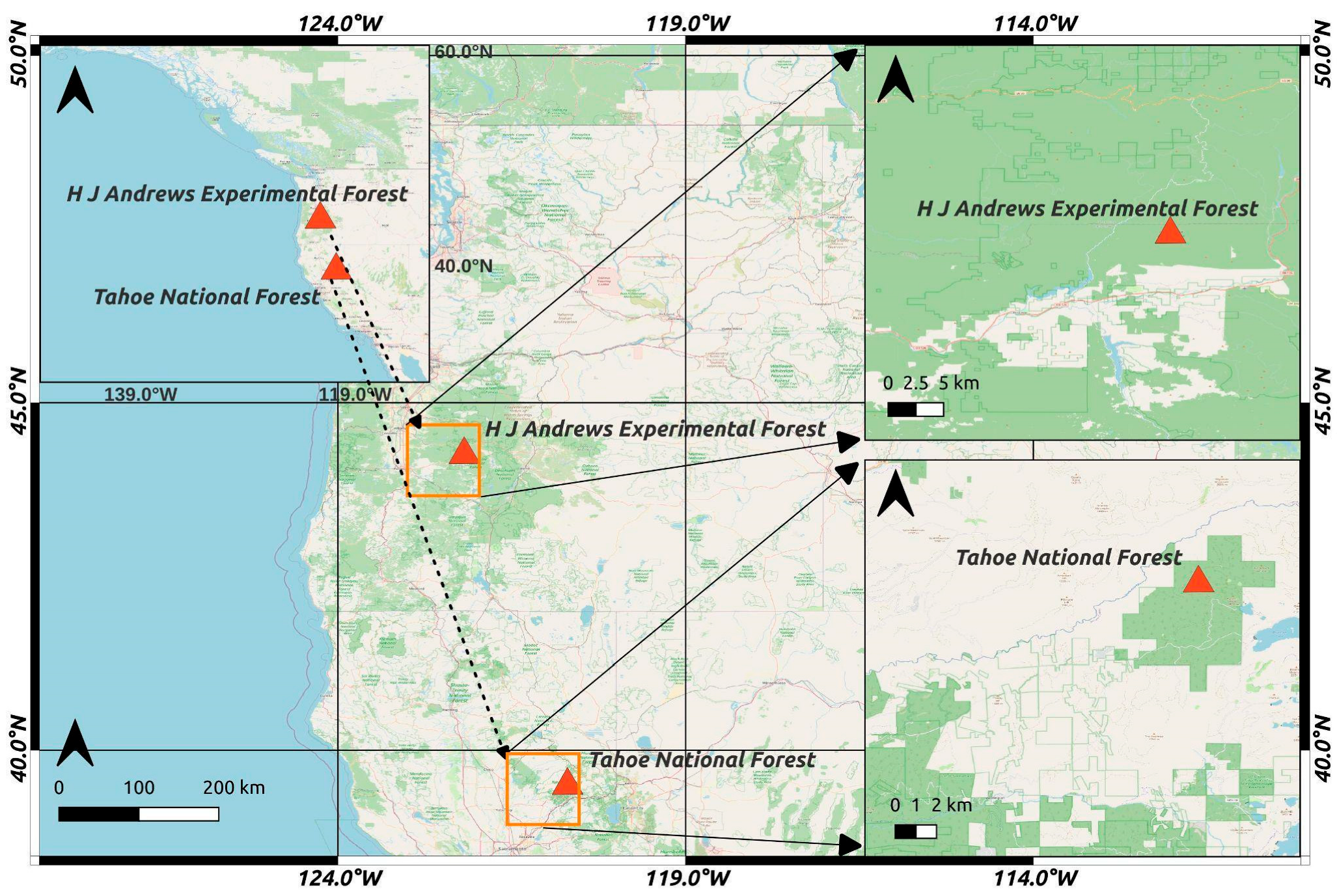
In this study, we use 3D LiDAR scenes of different forest areas (see
Figure 2) acquired with an airborne scanning platform. The first dataset we use for our research is the LiDAR scan of the Andrews Experimental Forest and the Willamette National Forest, which was acquired in August 2008 and is publicly available at OpenTopography. To conduct the experiments, we selected two test samples geographically distributed across the region from the complete scan. The samples represent LiDAR scans of forest regions, with most of the points belonging to the trees. The point density of the dataset is 12.23 points/m
2. Henceforth, the two Andrews Forest samples would be denoted as Andrews 1 and Andrews 2, whereas collectively, the dataset is referred to as Andrews Dataset. The second dataset is from the USFS Tahoe National Forest LiDAR scan acquired in 2014 and is also publicly available for download at the OpenTopography platform. We selected three samples from this dataset for performing our experiments. The point density of the dataset is 8.93 pts/m
2. Henceforth, the three samples of the Tahoe Forest would be denoted as Tahoe 1, Tahoe 2, and Tahoe 3, and collectively, the dataset would be denoted as Tahoe Dataset. All the selected scans have been shortlisted due to their complicated topography. It is important to note that trees form a complex geometry and are challenging to characterize.
2.2. Multivariate Empirical Mode Decomposition (MEMD)
The proposed MEMD approach utilizes only 3D spatial coordinates
x,
y, and
z as input attributes for each point in the point set. The multivariate EMD decomposes the input into components varying according to the spatial frequency in all three spatial dimensions.
where
are variable dimensions.
Typically, Equation (3) defines the EMD as an N-mode decomposition. The component denotes the Nth IMF, whereas the residual function represents the minimum variation in frequency. The residual function is crucial for the proposed approach as it hierarchically encodes the 3D geometrical shape and structure of the input LiDAR scene.
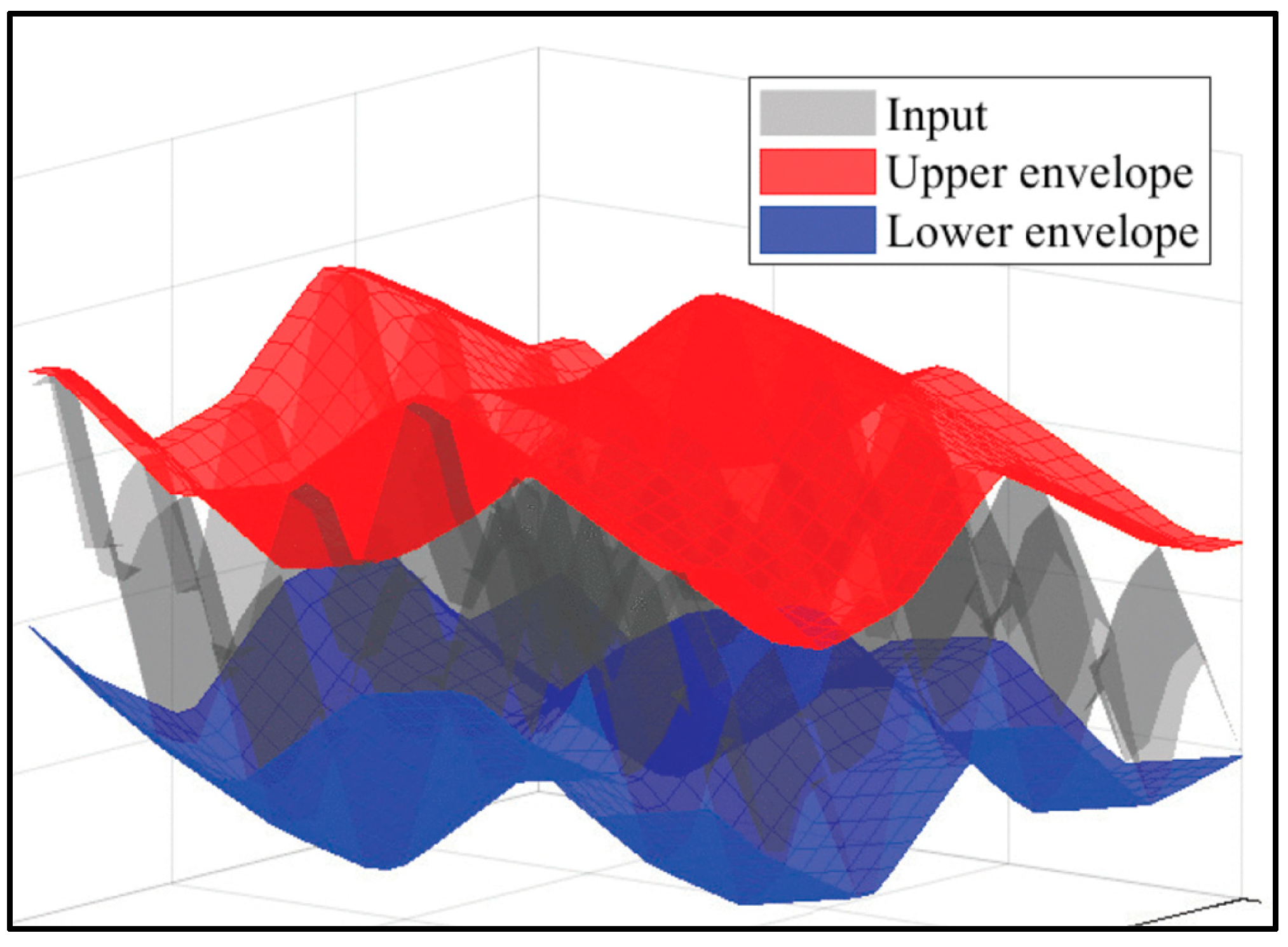
The derivation of IMFs is an iterative process of computing the average envelopes of the local minima and maxima points and subtracting the average envelope from the original signal. This process is called Sifting [
41] and is described in
Figure 3 for a 3D surface. It is crucial for distinguishing points that belong to a particular geometry or shape deformation in the whole scene (for, e.g., a point on the curvature or a point on the normal).
Conventionally, Sifting is performed iteratively, which can be challenging in some cases. It also becomes difficult to perform iterations with large matrix operations on large datasets. To overcome these problems, deep neural network-based implementations have proven to be successful. The conventional iterations are replaced by stacked convolution operations, and the difference in each iteration is backpropagated as an error to change the weights of the convolutional layers. Deep network-based implementations are scalable and flexible because the function representing the mathematical operations can be learned over the iterations in stacked convolutional layers.
2.3. Proposed ADCoSNet: Adaptive Decomposition-Driven Compressive Sensing-Based Neural Geometric Reconstruction
In
Figure 4, we present the holistic workflow of our proposed ADCoSNet framework.
2.3.1. Understanding MEMD in a Compressive Sensing Framework
The conventional Compressive Sensing approach solves the problem mentioned in Equation (1), reformulated again as Equation (4) below. This problem is also termed as
minimization problem and is used as a relaxed alternative to the
minimization problem, which is NP-hard to solve. Prior research has shown that near-perfect CS-based reconstruction can be obtained by solving the
minimization problem [
42].
where
st means “subject to the condition”,
is a given signal and
represents the measurement vector of
, which can be expressed as
, where
is the sensing matrix,
and
,
with
.
represents the number of points in the point sets and
N represents the number of sampled points. Equation (4) forms an underdetermined system of equations since
M <
N and is solved by optimization theory using linear programming.
Now, replacing
p in Equation (4) with the tri-variate signal
f from Equation (3), we achieve Equation (5) as described below:
Equation (5) represents the proposed ADCoSNet framework with
f =
, for modeling the CS-based reconstruction of decomposed components. Equation (5) forms the backbone of the Multivariate Empirical Mode Decomposition module of our proposed ADCoSNet architecture (Refer to
Figure 4). Equation (5) can be solved by separating the trivariate (3D point set varying with
x,
y,
z) signal into three 1D signals because the
x,
y, and
z attributes are independent. This also reduces the computation time to a great extent.
where
n = {
x,
y,
z},
=
,
m = number of elements in
and
represents the over-complete dictionary or the sensing matrix. The sensing matrix,
, is computed as defined in Equation (1), also defined as Equation (7) below for reference.
Based on Equation (6), Equation (7) can be reframed as Equation (8) below:
The objective function described in Equations (6) and (8) forms the basis for the proposed ADCoSNet’s architecture, as illustrated in
Figure 4.
2.3.2. Training the Proposed ADCoSNet Architecture
In this section, we discuss the training of our proposed deep network for the reconstruction of CS measurements of the 3D LiDAR point cloud in detail. For all the cases, we use the network architecture, as shown in
Figure 4, for analyzing the robustness and consistency of our novel ADCoSNet architecture.
For the two selected datasets, batches of size 1024 points have been extracted from the 3D LiDAR scenes. Each point in the point set comprises x, y, z as the raw attributes. These pointsets form the labels of our training set. The corresponding CS measurements of the pointsets are obtained depending on the CS measurement ratios, and these measurements form the inputs of our training set. For example, if the selected CS measurement ratio is 0.50, the size of a point set forming the label would be (1024, 3), and the size of the input point set would be (512, 3). We present comprehensive 3D reconstruction results using our proposed ADCoSNet for the two selected datasets for five different CS Measurement ratios—0.75, 0.50, 0.25, 0.10, and 0.04—implying sampling of points equal to 75%, 50%, 25%, 10% and 4% from the input data for training the network. The measurement set is obtained by , where denotes the sensing matrix. The training pair can be represented as (qi, pi) or (Api, pi) or (ϕψpi, pi), where pi, qi represents the ith sample of the vector sets and , respectively. Hence, the number of measurements for the CS measurement ratio of 0.75, 0.50, 0.25, 0.10, and 0.04 translates to n = 768, 512, 256, 102, and 40, respectively.
We performed experiments for various CS ratios by testing a deep learning model for individual CS ratios. Deep learning models are implemented using PyTorch [
43]. The
loss function averaged over all the point sets is selected as a reconstruction metric.
describes the loss function and is optimized using backpropagation during the training.
M in
represents the total number of point sets in the training set,
represents the
ith point set, and
=
represents the output of the proposed network corresponding to the
ith point set. The batch size is consistent at 16 while training and the learning rate is 0.001. A dropout layer prepends on the output layer to enhance the network’s generalization and avoids overfitting while training. The training for all the networks for five different CS measurement ratios and the selected datasets is performed on the Nvidia Tesla K40 GPU available on the Google Cloud Platform.
3. Results
In this section, the proposed approach is comprehensively evaluated. The experiments include the computation and statistical analysis of the results generated by the adaptive decomposition of the 3D LiDAR scenes. This is followed by the CS-based 3D reconstruction of the point cloud from the sparse measurements obtained by using only the least spatially varying component (last IMF) without deforming the nature of the point cloud. We present a quantitative and qualitative evaluation of the reconstructed 3D scenes for five different CS measurement ratios—{0.75, 0.50, 0.25, 0.10, 0.04} based on performance metrics.
3.1. Implementation Details
The implementations are performed on a Google Cloud Platform instance with a CPU of RAM 30GiB and Nvidia GPUs. The decomposition components for each sample resulted in IMFs with decreasing variation in the spatial frequency. The initial IMFs capture high spatial frequency components and represent a more fluctuating part than the last IMFs. This section analyzes four initial IMFs, four last IMFs, and the filtered signal.
For the Compressive Sensing-based reconstruction, we have used random Gaussian matrices as the sampling basis () for sampling the points in the 3D space. The random Gaussian matrices are proved to follow the restricted isometry property (RIP), thus forming a natural choice for sampling. The sampled points and the input data points form the training pair, {hi, ki}, where hi represents the output of the adaptive decomposition algorithm. The batch size is set to 16, the learning rate to 0.001. The adaptive moment estimation (Adam) is set as an optimizer and mean squared error (MSE) as the loss function throughout the experiments.
Initially, we experimented using the l1 norm as a loss function but observed that MSE converged better than the l1 norm. The quantitative evaluation of the results is performed using PSNR (Peak Signal to Noise Ratio), RMSE (Root Mean Squared Error), and Hausdorff point cloud-to-cloud distance as performance metrics. Although PSNR is used as a metric for quantifying reconstruction results, it lacks human perception of comprehending real-world geometries. The RMSE is a statistical metric corresponding to the closeness of reconstructed output with the actual output based on the l2 norm. Hausdorff distance (H.D.) is a widely used metric for geometrical shape analysis which defines the closeness between similar points in the 3D space for the two sets.
Given two point sets
P = {
p1,
p2, …
pn} and
Q = {
q1,
q2, …
qn}, Hausdorff distance between
P and
Q—
HD(
P,
Q), is defined as:
where
h(
P,
Q) =
(
(
)) and,
h(
Q,
P) =
(
(
)).
Mathematically, as formulated in Equation (9), it is estimated as the maximum Euclidean distance from a point in one set to the closest point in the other set. In terms of 3D point sets, H.D. represents the maximum deviation between two 3D point sets, measuring how far two point sets are from each other [
44]. Hence, an
HD(
P,
Q) = 0 implies that
P and
Q are identical. Ideally, for a perfect reconstruction, it is expected to have a high PSNR with low values for RMSE and Hausdorff distance.
3.2. Adaptive Decompositions as Data-Driven Transforms
To interpret the results of adaptive decomposition on the point sets, we implemented and analyzed Multivariate Empirical Mode Decomposition on the 3D point sets. Qualitative visualization is based on perceptual examination of the estimated IMFs, while statistical significance based on feature relevance is the basis for quantitative evaluation.
3.2.1. Visual Interpretation of the Adaptive Decomposition Components
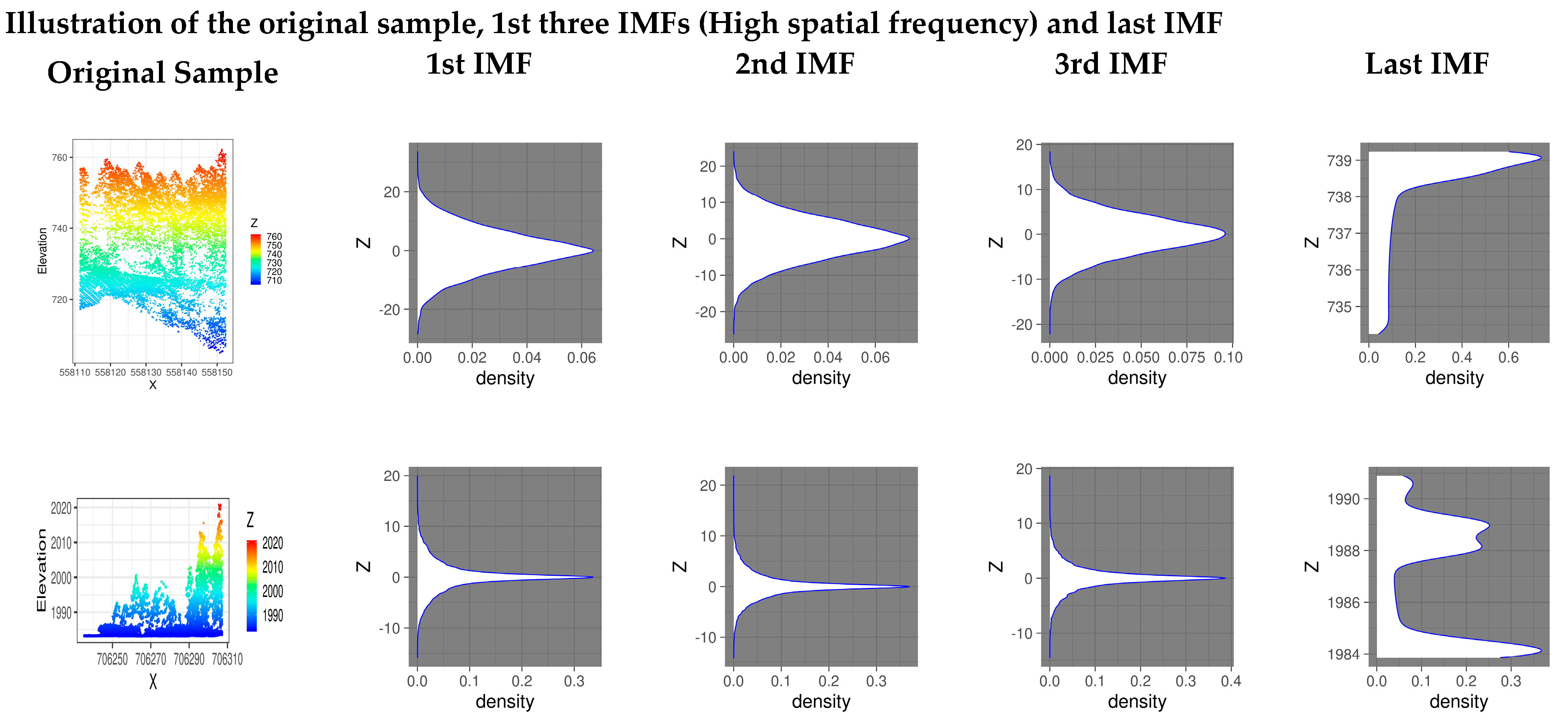
The initial work on the interpretation of EMD-derived components for white noise [
45] is the basis for our observation of the behavior of MEMD-derived IMFs. The initial IMFs follow approximately a normal distribution (refer to
Figure 5). It is evident from the visualization of the last IMF that it is a close approximation of the input LiDAR point set in terms of the overall geometrical shape.
3.2.2. Investigation of Statistical Significance of the Intrinsic Mode Functions (IMFs)
Table 1 presents the quantitative analysis for understanding the statistical significance of the MEMD-derived IMFs. The statistical metrics are chosen based on the widely used feature relevance metrics—Peak Signal to Noise Ratio (PSNR), Mutual Information (MI), and Pearson’s Correlation Coefficient (
r). We observe that out of all IMFs, the last IMF prominently captures the complete information regarding geometrical shape and structure.
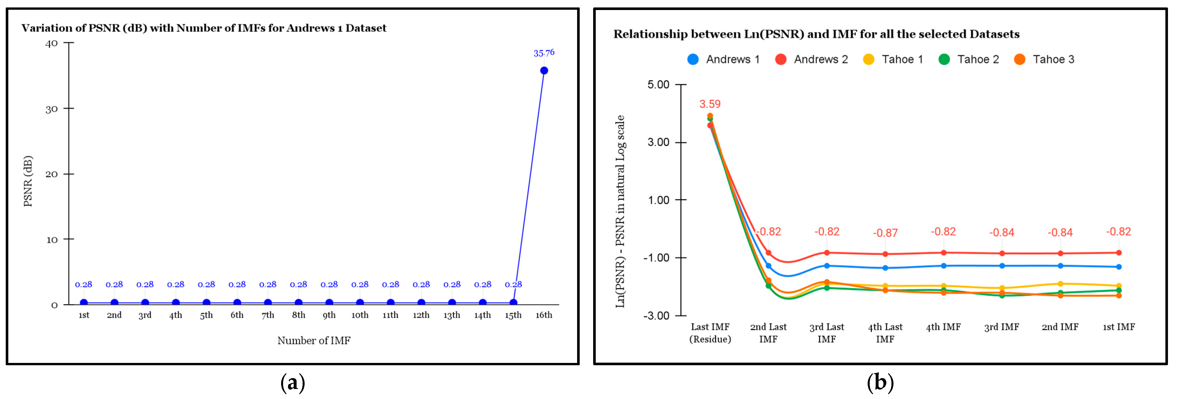
Figure 6a illustrates the variation in PSNR with the number of IMF. The last IMF has a significant PSNR compared to the rest of the IMFs.
Figure 6b justifies this trend for all the selected datasets. The maximum PSNR of around 50.8 dB and 36.2 dB is observed for Tahoe 1 and Andrews 1, respectively.
3.3. Compressive Sensing-Based Reconstruction of 3D LiDAR Point Clouds
The CS-based recovery is performed with the filtered signal obtained after the EMD to generate sparse representations based on different CS measurement ratios. These sparse representations are then used to reconstruct the original 3D LiDAR point cloud. The Compressive Sensing-based reconstruction of point cloud data comprises four steps:
Generating the filtered input signal from the MEMD derived Intrinsic Mode Functions (IMFs).
Transforming the filtered signal to a transformed vector space using representation basis () to obtain a low-dimensional representation.
Sampling the transformed signal using sampling basis () to obtain samples representing a low-dimensional sparse approximation of the complete 3D scene.
Reconstructing the point cloud by solving the optimization problem as the proposed deep convolutional 3D reconstruction network.
A detailed analysis of quantitative and qualitative results is presented in the following subsections.
3.3.1. Illustration of the Reconstructed 3D LiDAR Point Clouds Using the Proposed ADCoSNet for Different CS Measurement Ratios Based on Qualitative Visualization
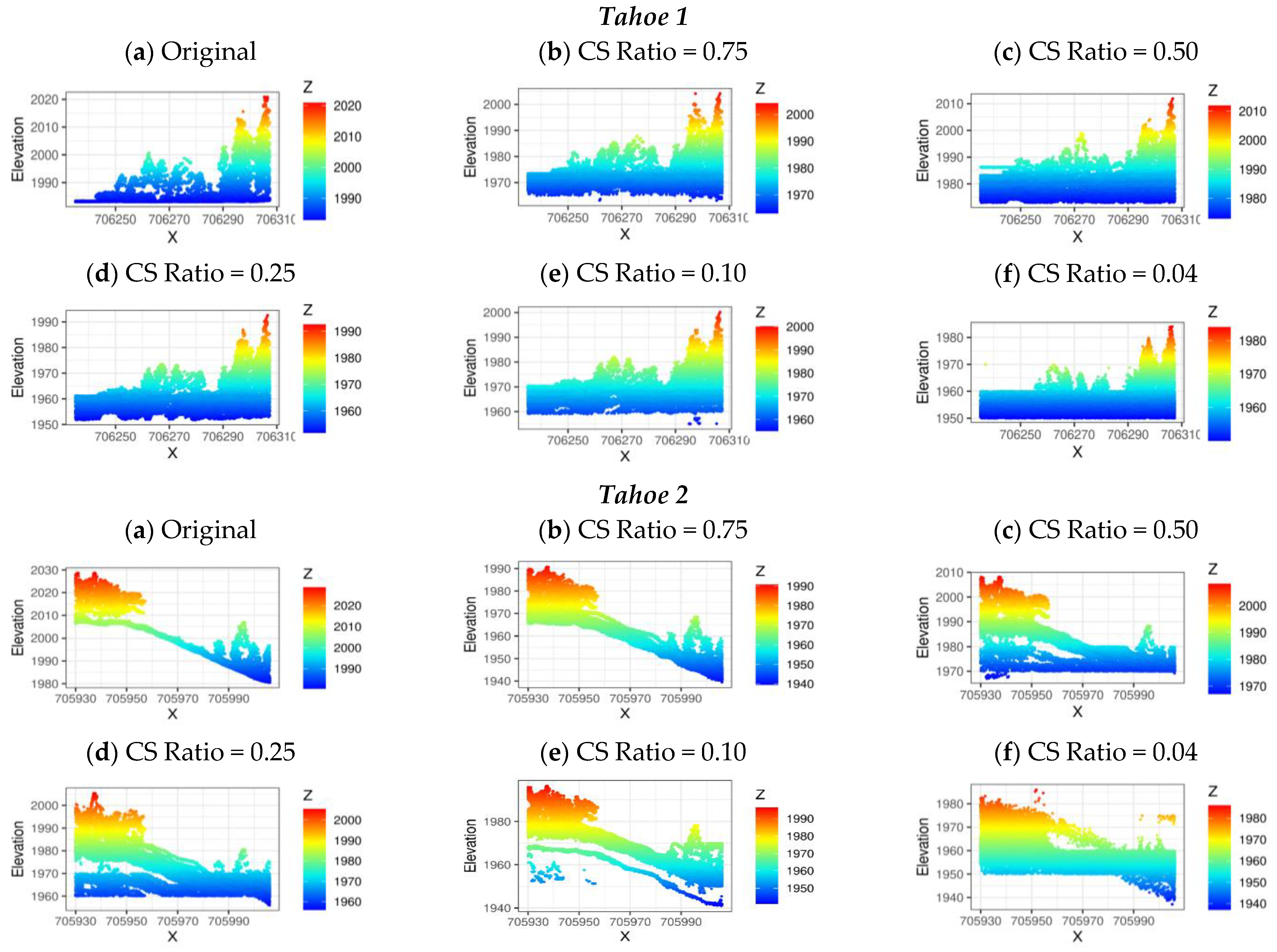
Figure 7 and
Figure 8 illustrate the reconstructed 3D LiDAR point clouds with the original 3D LiDAR point clouds for different CS measurement ratios—4%, 10%, 25%, 50%, and 75%. The legend to the right of the illustrations indicates the elevation symbology with respect to the cartesian coordinate (
x). It is observed that the reconstruction fidelity of the reconstructed 3D LiDAR point clouds decreases with a decrease in the number of measurements used for the reconstruction. It is justified as the reconstruction accuracy will improve with the availability of more measurements.
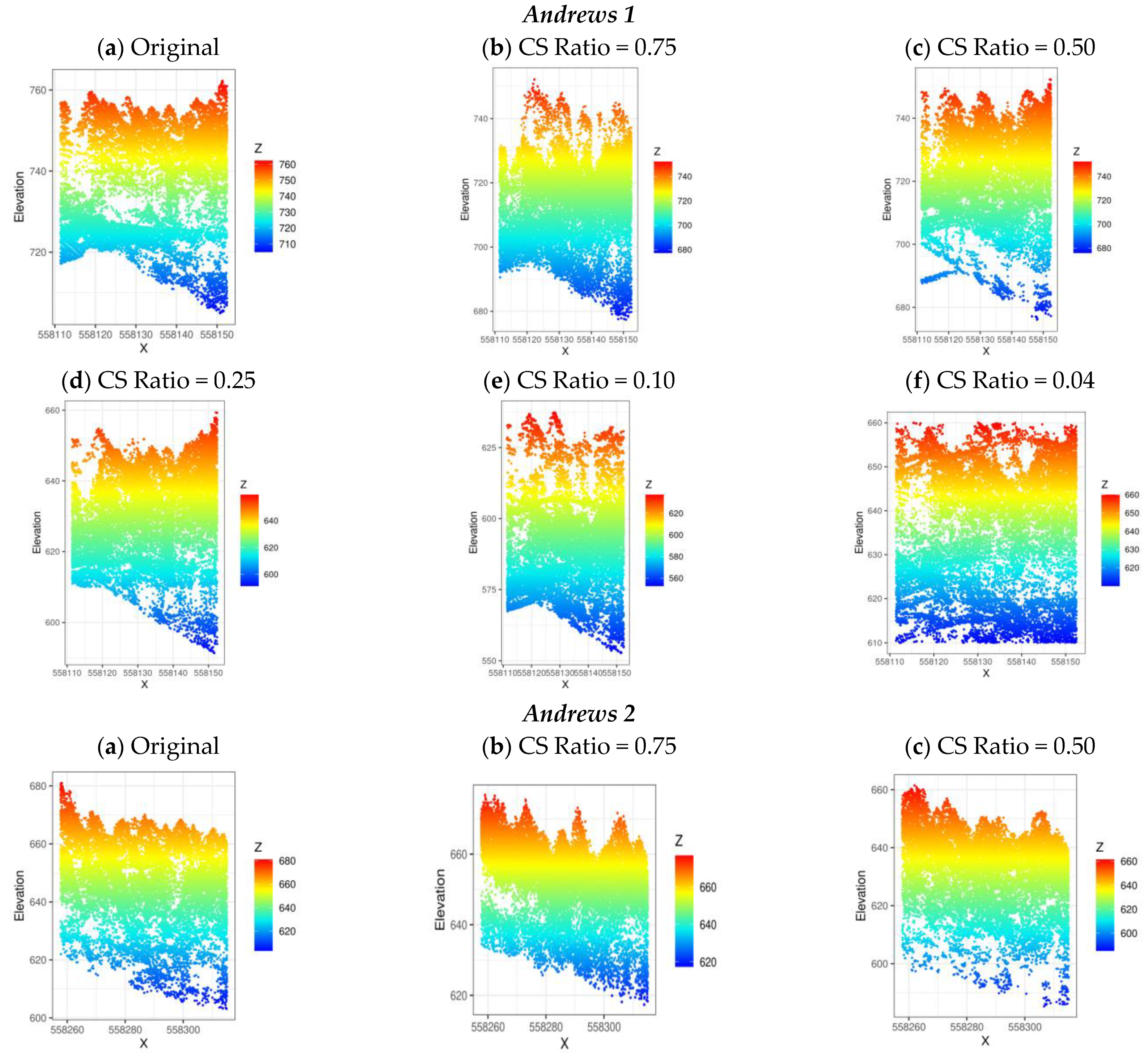
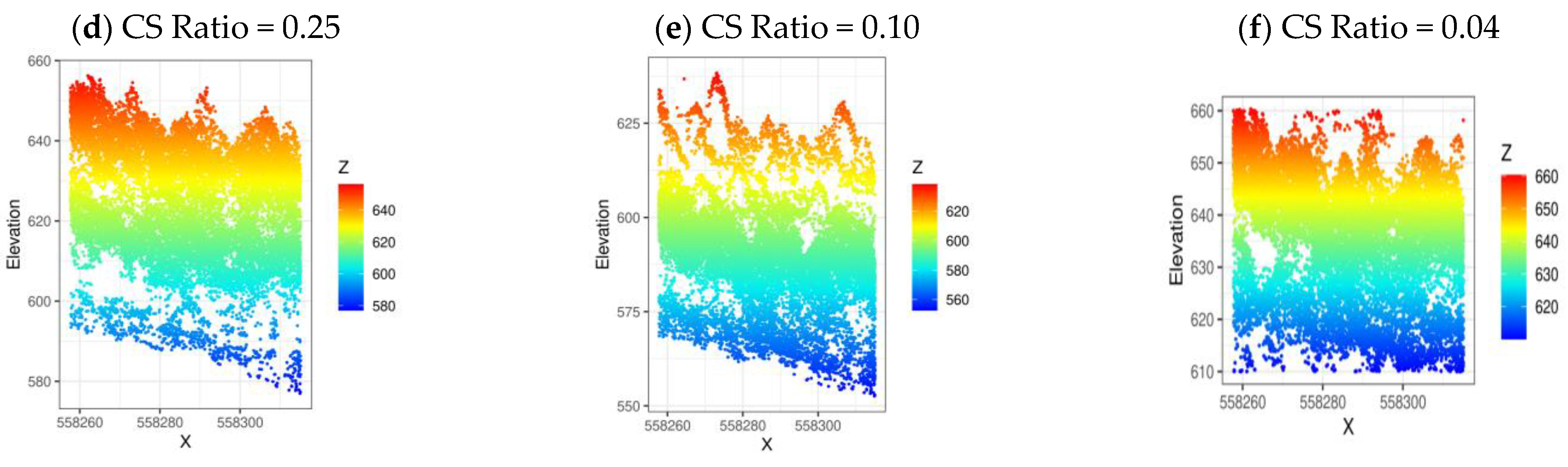
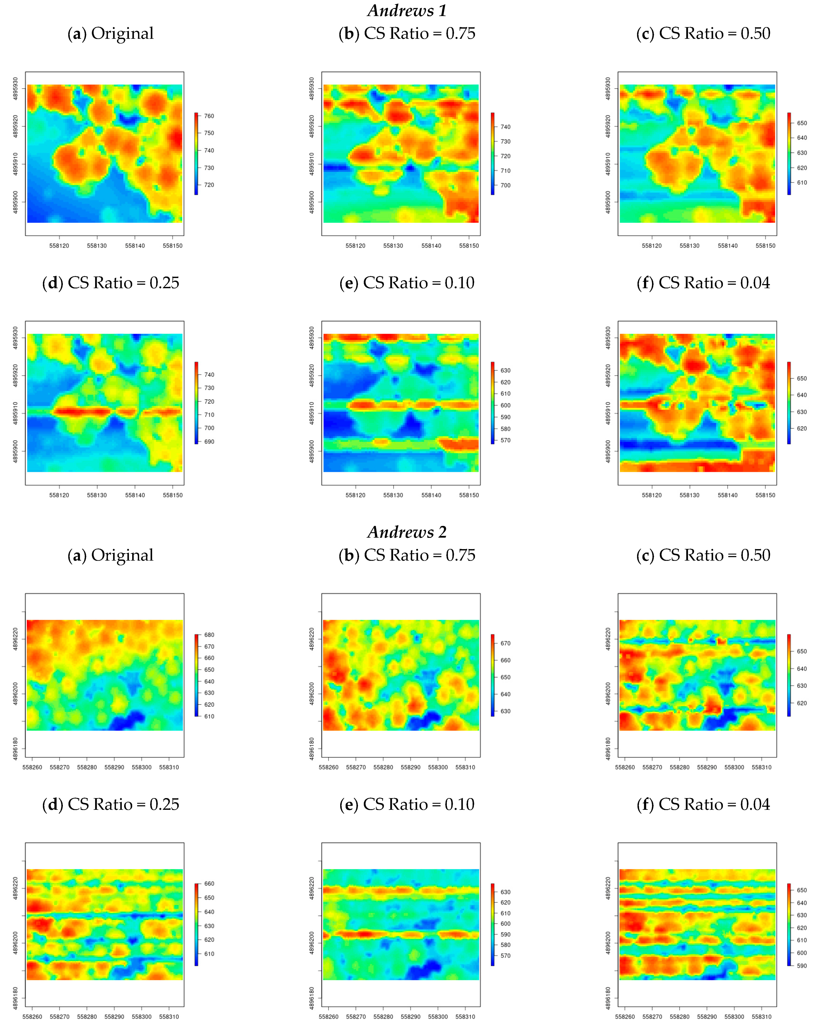
Figure 7 visualizes the reconstructed point clouds for the Andrews 1 and Adrews 2 test sites. From the perspective of 3D LiDAR data, elevation information is a differentiating factor for analysis. As evident from the illustrations for both the Andrews test site (see
Figure 7), the variation in topography is less distinguishable as the CS ratio decreases. Both the Andrews test sites are rich in high elevation and dense points attributed to the presence of vegetation. It is observed that the tree canopy structure is preserved for high CS ratios—75%, 50%, and 25%; however, it is distorted significantly for CS ratios—10% and 4%.
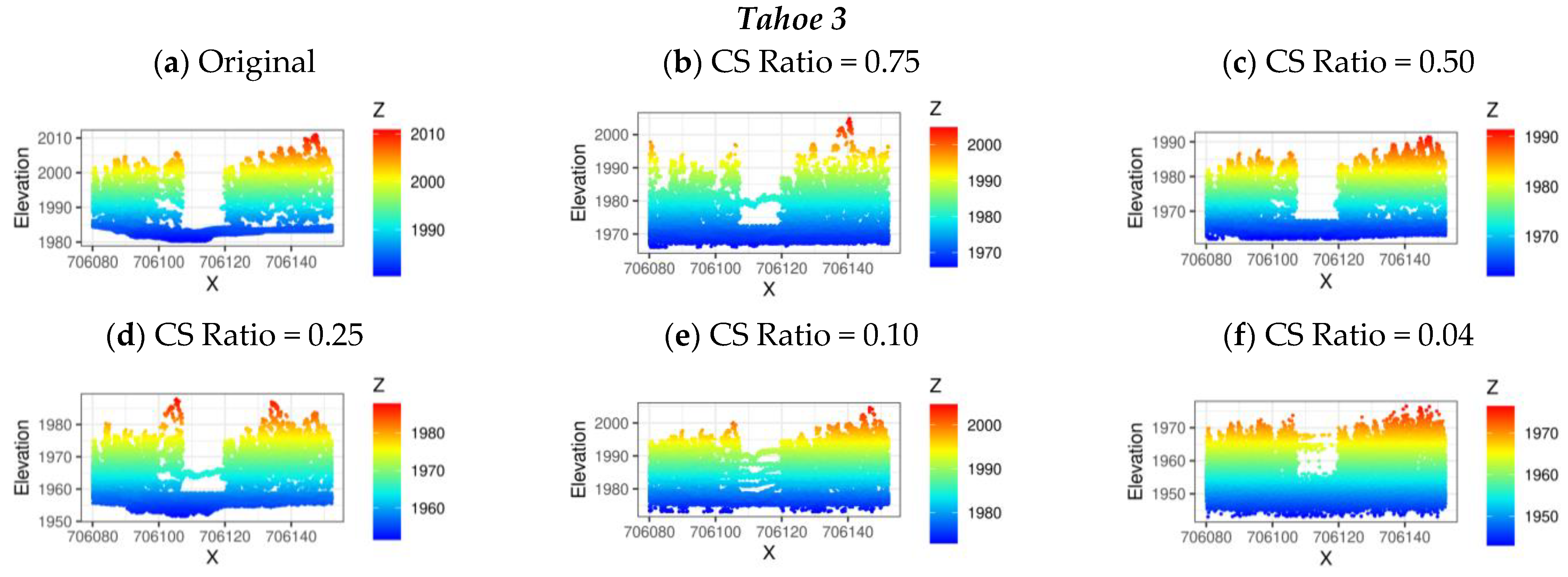
Figure 8 illustrates the reconstruction results for the Tahoe test sites. For Tahoe 1 site, the reconstruction is consistent for all the selected CS ratios. This is possible due to the flat topography of the Tahoe 1 test site. For the Tahoe 2 site, the reconstruction seems to be consistent with the original only for the CS ratio of 75%. The reconstruction results for CS ratios of 50%, 25%, 10%, and 4% seem to be distorted, attributed to the hilly topography. Similar to Tahoe 1, Tahoe 3 also poses a flat topography with a discontinuity of forest canopy in between. It is observed that for Tahoe 3, the reconstruction for CS ratios—75% and 50%—is close to the original; however, it is significantly distorted for the other CS ratios.
3.3.2. Quantitative Investigation of the Efficacy of the Proposed ADCoSNet for 3D Reconstruction
Table 2 presents a quantitative evaluation of the reconstructed LiDAR point clouds using our proposed ADCoSNet for the selected Andrews and Tahoe datasets based on performance metrics. It is evident from
Table 2 that the maximum PSNR achieved for reconstruction is 48.96 dB, and the minimum RMSE is 7.21 for the Tahoe 1 sample corresponding to a CS measurement ratio of 0.75. The Hausdorff distance for this reconstruction is 11.19.
Although both the selected datasets are 3D LiDAR scans of forests, there is a difference in quantitative results. This is attributed to different geographical locations as well as the type of forests. From
Table 2, it is also observed that the reconstruction RMSE for Andrews 1 dataset surges for CS ratios—0.25, 0.10, and 0.04 emphasizing that these CS measurement ratios would not be a suitable choice for generating sparse representations. The increase in reconstruction error could possibly be due to the hilly or mountainous topography of the Andrews 1 site.
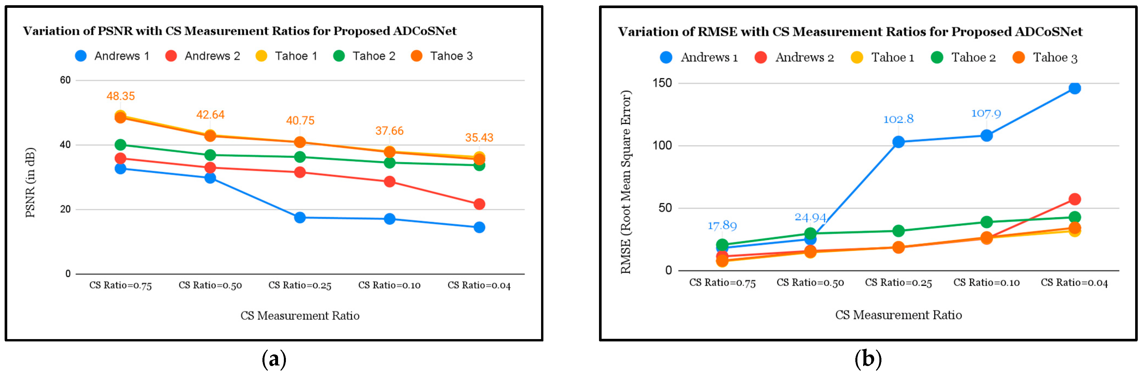
We also observe from
Figure 9a,b that the performance of 3D reconstruction enhances with variation in CS measurement ratio, i.e., number of samples used for reconstruction. From
Figure 9a, the PSNR decreases with a decrease in the CS measurement ratio, whereas from
Figure 9b, the RMSE increases with a decrease in the CS measurement ratio. This is justified as more samples would lead to better reconstruction results. These results are significant in understanding the behavior of CS-based reconstruction with a measurement ratio and the limit to which sampling could be performed for achieving a particular reconstruction performance.
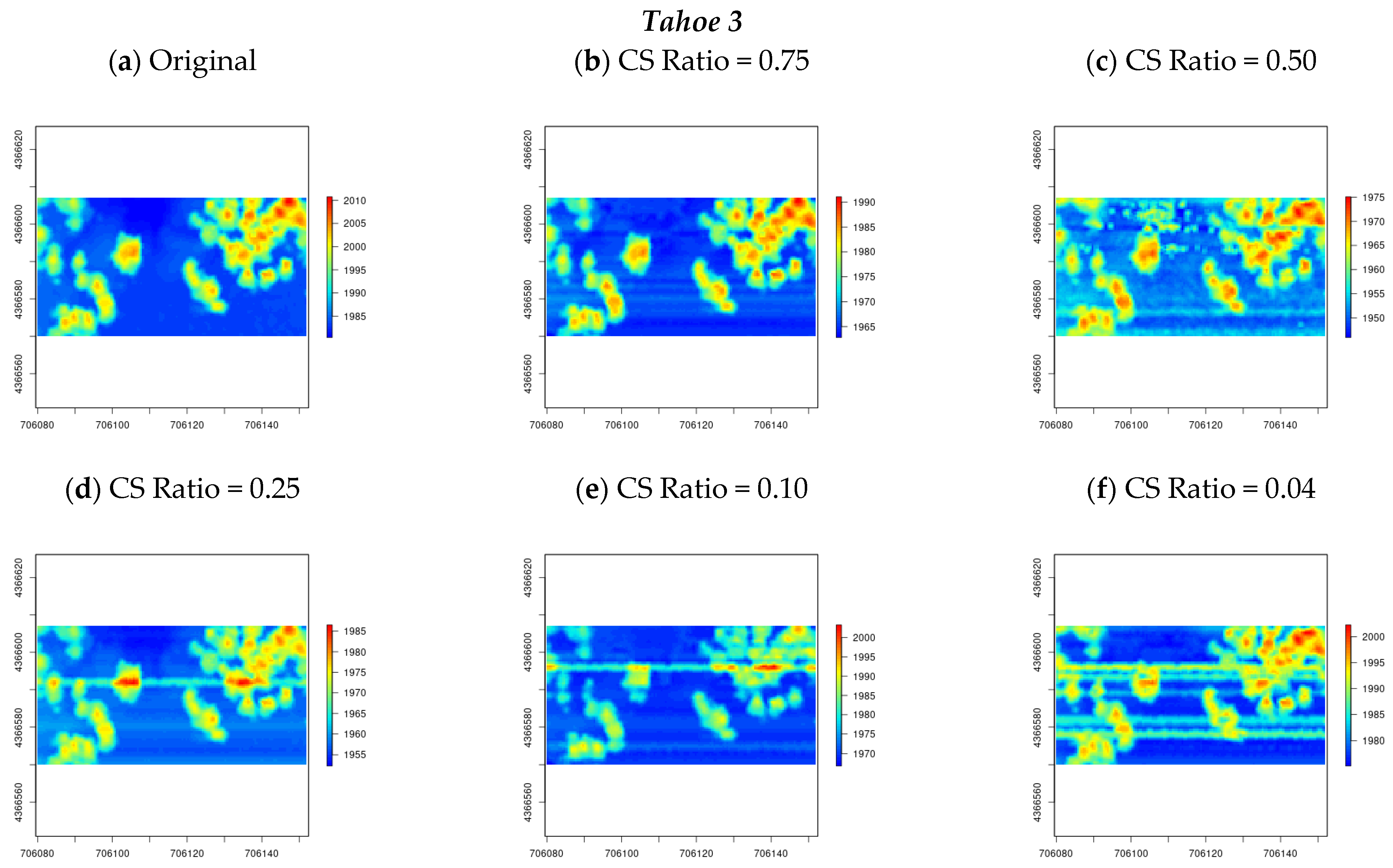
3.3.3. Evaluation of Reconstructed LiDAR Point Clouds Based on the LiDAR-Derived Canopy Height Model (CHM)
From the perspective of LiDAR-derived results useful for forest analysis, the Canopy Height Model (CHM) plays a significant role. The CHM plot is used to visualize vegetation height as a continuous surface where each pixel in the plot represents the normalized tree height above the ground topography. To understand the efficacy of the proposed ADCoSNet, the CHM plots for all five sample datasets (Andrews and Tahoe datasets) are generated from the reconstructed 3D LiDAR point clouds.
Intuitively, it is expected that most of the CHM representations would consist of tree canopy cover as the test samples are selected from the forest. The ground truth CHM is derived from the Digital Surface Model (DSM) available with the OpenTopography platform, and individual DSMs for the samples were clipped based on the extent of the region. We believe such a comparison would help analyze the efficacy of our proposed approach at a local surface level. In
Figure 10 (results for the Andrews dataset) and
Figure 11 (results for the Tahoe dataset), the CHM illustrations derived from the reconstructed LiDAR point cloud for different CS measurement ratios are visualized.
For both the Andrews and Tahoe dataset (refer to
Figure 10 and
Figure 11), it is evident that the CHM plots for the original are visually close to the plots for the reconstructed point clouds with CS measurement ratios of 0.75, 0.50, and 0.25. However, for the CS measurement ratio of 0.10 and 0.04, it is observed that there is a horizontal line in the generated raster. This could be possible due to the effect of one of the EMD-derived IMFs in the reconstructed LiDAR point cloud. Moreover, for all the test sites, the high-elevation region (points belonging to high vegetation, i.e., pixels represented by the red color in the illustration) and the low-elevation region (points belonging to ground, i.e., pixels represented by the blue color in the illustration) are observed to be more distorted as compared to the points with medium elevation. This could be due to the implementation of the MEMD which inherently involves averaging the maximum and minimum envelopes of the input data (also known as Sifting—refer to
Section 2.2).
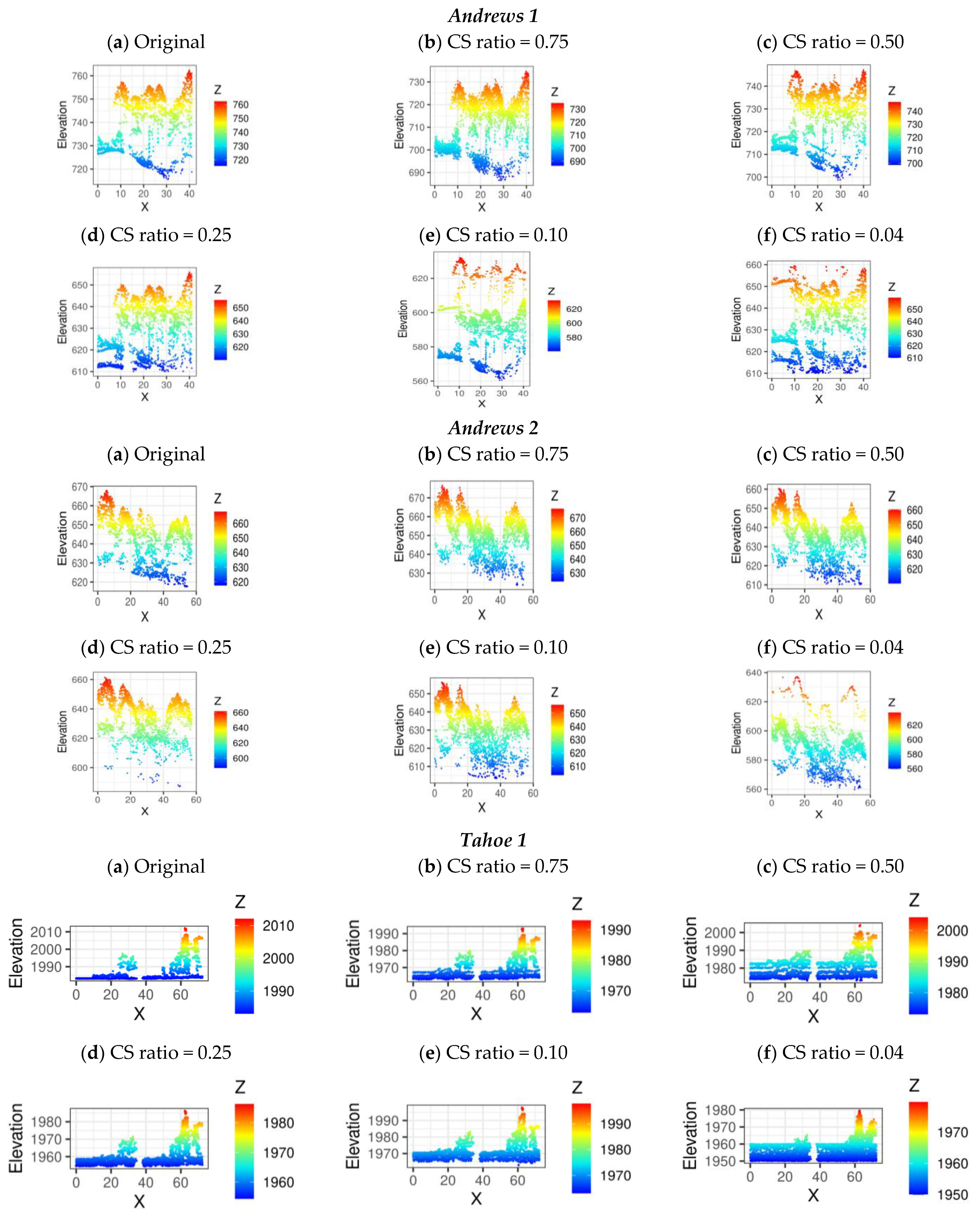
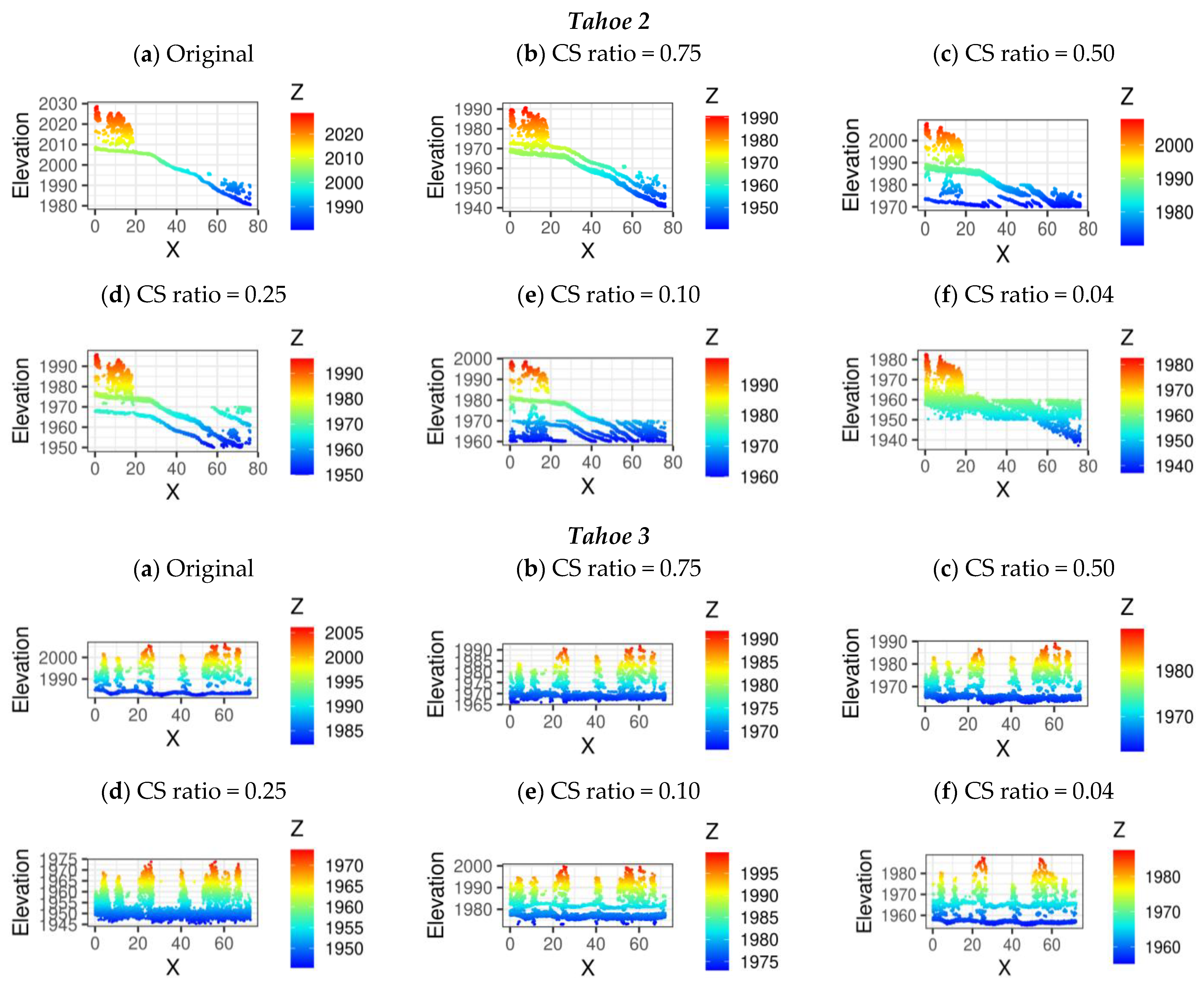
3.3.4. Investigation of the Efficacy of the Proposed ADCoSNet Architecture for Reconstruction Based on LiDAR Derived Elevation Results (2D Vertical Elevation Profile)
To further evaluate the robustness and reconstruction fidelity, we observed the 2D vertical elevation profile for a subset of the original and reconstructed point clouds using the proposed ADCoSNet. The 2D vertical elevation profile is a significant LiDAR point cloud-derived result and is prominently used in evaluating the accurate topological profile of the region. Visual inspection based on the elevation range reveals (see
Figure 12) that the 2D vertical elevation profile follows the reconstruction results. In addition, the figures show that the reconstruction at the local level is consistent with the overall reconstruction. However, there is a slight difference in the range of elevation values for the CS measurement ratios equal to 0.10 and 0.04 (plots (e) and (f) of
Figure 12).
As observable from
Figure 12, the 2D vertical elevation profile for the point clouds reconstructed using the proposed ADCoSNet follows the geometric profile as the original LiDAR point cloud. While we observe acute changes in the crown reconstruction for the forest samples’ trees, the broad elevation range of the reconstructed point cloud is consistent with the original LiDAR point cloud.
3.3.5. Enhancement in the Reconstruction Accuracy by Using Multivariate Empirical Mode Decomposition
Regarding machine learning and deep neural networks, ablation study experiments typically measure the network’s performance after removing or replacing the network components.
Table 3 presents an ablation study for analyzing the enhancement in reconstruction performance of our proposed approach of using deep convolutional compressive sensing reconstruction networks
with and
without EMD-derived features. It is evident that MEMD enhances the 3D reconstruction performance by approximately 8 dB (40.94 dB
48.96 dB). It is envisaged that this will help understand the advantage put forth using multivariate Empirical Mode Decomposition as a basis for transformation and the convolutional features.
4. Discussion
The proposed ADCoSNet framework is meticulously evaluated to analyze the reconstruction of forest 3D LiDAR scans. Based on the qualitative and quantitative analysis of a total of five test sites—Andrews 1, Andrews 2, Tahoe 1, Tahoe 2, and Tahoe 3, it is understood that the proposed ADCoSNet is capable of reconstructing point clouds accurately for CS ratios of 75%, 50%, and 25%. However, there is a distortion within certain limits for the CS ratios of 10% and 4% for some test sites. The CHM analysis shows that the reconstruction accuracy depends on the test site’s topography. This justifies the adaptivity introduced by the MEMD in a typical compressive sensing framework with a data-agnostic transformation function in Compressive Sensing framework.
It is expected that the LiDAR-derived forest-related results, such as the relative height of the vegetation, canopy density model (CDM), etc., can further be evaluated to investigate the accuracy of the reconstructed point clouds. However, these experiments are not performed in this research. The ablation study investigates the performance enhancement due to incorporating MEMD in the proposed ADCoSNet. It is observed that using MEMD-derived Residue function for Compressive Sensing based sparse recovery leads to an overall increase of 8 dB in the reconstruction results. Additionally, we highlight the following significant points to support our hypothesis of using a data-driven transform in a convolutional Compressive Sensing framework:
- (1)
The residual function derived from the Multivariate Empirical Mode Decomposition (MEMD) approximates the total variation in the 3D geometry of the point cloud. Based on statistical significance, the residue function has greater mutual information than other IMFs because its overall structure is closest to the raw LiDAR point cloud.
- (2)
It can be observed that the mutual information of the residue function is very close to the original 3D profile. As far as we know, the visualization and application of MEMD results for LiDAR point cloud data is a novel contribution and could potentially be an effective approach for large-scale 3D reconstruction in different areas. Moreover, due to its learning ability in data distribution, the proposed approach is expected to be effective in relatively heterogeneous environments, such as urban areas.
- (3)
Deep convolutional network-based CS reconstruction of LiDAR point cloud data possesses excellent opportunities as an alternative to the iterative CS reconstruction approaches. The convolutional features extracted hierarchically by the convolutional layer stack seem to be an accurate approximation of the measurement samples. They could be used with sparse coding problems for 3D LiDAR point clouds.
- (4)
It is evident from the illustrations of
Figure 10 and
Figure 11 that the CHMs generated for the reconstructed point clouds are close to the CHMs for the original sample. Additionally, it is observed that for the test sites with topographical discontinuity, such as valley (from Andrews 1 and Tahoe 2), the proposed ADCoSNet approach can reconstruct the 3D LiDAR point cloud with decent accuracy.
- (5)
Future Research Directions: It would be interesting to observe the behavior of the adaptive decomposition-derived IMFs for temporal LiDAR data to incorporate data-centric features for geometry processing. Another compelling research direction is to process the 3D LiDAR point set in less time with comparable accuracy. This poses an immense potential for infield processing using hand-held computing devices with less storage and computing power. Further, in the future, onboard processing is envisaged on the streaming LiDAR data. In such a situation, processing the data with limited storage and computing power requires compression, enabling it to send processed information instead of raw LiDAR point cloud directly.
5. Conclusions
In this paper, the adaptive decomposition approach—Empirical Mode Decomposition, also called the Hilbert–Huang Transformation—is implemented in a Compressive Sensing framework. Empirical Mode Decomposition is a data-driven transform that learns adaptive decompositions based on the input data, unlike Fourier and wavelet transforms with a fixed structure. EMD is highly important for 3D forest LiDAR, as it has proven effective for non-linear, local, and non-stationary signals. The proposed approach advocates a data-centric implementation that focuses on the input data for the deep learning neural model. The EMD-derived mode decompositions capture the variations of spatial frequency in 3D space, where the last IMF is important as a feature set. This feature set is merged with the convolutional feature set to generate sparse representations using the proposed ADCoSNet. The ADCoSNet replaces the conventional iterative-based CS solvers and is scalable for multi-resolution analysis. Moreover, the proposed approach generates adaptive sparse representations to account for local variations in a forest environment. These variations are captured as spatial discontinuities in the relatively homogeneous forest environment consisting only of vegetation cover. Furthermore, it is expected that a learning-based implementation of the proposed ADCoSNet will allow the generalizability of the approach to other forest environments.
It is noticed that the proposed approach can reconstruct the 3D LiDAR point clouds with the best PSNR value and RMSE of ~49 dB and 7.21 (Tahoe 1), respectively, for the CS measurement ratio of 0.75. The worst reconstruction is achieved with a PSNR of ~14 dB for the CS measurement ratio of 0.04 with an RMSE of 145.8 (Andrews 1). The results obtained with the proposed approach are compared with the original 3D LiDAR point clouds based on statistical significance and feature relevance metrics for several CS ratios. To our knowledge, applying adaptive decomposition algorithms in a deep convolutional compressive sensing framework for the geometric reconstruction of 3D LiDAR point clouds is a new contribution. We envisage using our approach in applications that involve near real-time processing of 3D LiDAR point clouds based on onboard computing for rapid 3D reconstruction. This poses an immense potential for infield processing using hand-held computing devices with less storage and computing power for quick file validation. Furthermore, improvement in reconstruction by including local geometrical and topographical features of the 3D LiDAR point cloud is envisioned as a future research direction.
Author Contributions
Conceptualization, R.C.S. and S.S.D.; methodology, R.C.S. and S.S.D.; software, R.C.S.; validation, R.C.S. and S.S.D.; formal analysis, R.C.S.; investigation, R.C.S.; resources, R.C.S. and S.S.D.; data curation, R.C.S.; writing—original draft, R.C.S.; writing—review & editing, S.S.D.; visualization, R.C.S.; supervision, S.S.D.; project administration, S.S.D.; All authors have read and agreed to the published version of the manuscript.
Funding
This research received no external funding.
Data Availability Statement
Acknowledgments
The authors, express their gratitude towards the OpenTopography Facility with support from the National Science Foundation for publishing the open LiDAR data. The NSF OpenTopography Facility provides the 2014 USFS Tahoe National Forest LiDAR and Andrews Experimental Forest and Willamette National Forest LiDAR (Aug 2008) datasets. The authors also express their gratitude to the Google Cloud Research Programs team for awarding the Google Cloud Research Credits with the award GCP19980904 to use the high-end computing facility for implementing the architectures.
Conflicts of Interest
The authors declare no conflict of interest.
References
- Mallat, S.; Zhang, Z. Matching pursuits with time-frequency dictionaries. IEEE Trans. Signal Process 1993, 41, 3397–3415. [Google Scholar] [CrossRef] [Green Version]
- Xu, Q.; Sheng, Z.; Fang, Y.; Zhang, L. Measurement Matrix Optimization for Compressed Sensing System with Constructed Dictionary via Takenaka–Malmquist Functions. Sensors 2021, 21, 1229. [Google Scholar] [CrossRef] [PubMed]
- Huang, N.E.; Shen, Z.; Long, S.R.; Wu, M.C.; Shih, H.H.; Zheng, Q.; Yen, N.-C.; Tung, C.C.; Liu, H.H. The empirical mode decomposition and the Hilbert spectrum for nonlinear and non-stationary time series analysis. Proc. R. Soc. A 1996, 454, 903–995. [Google Scholar] [CrossRef]
- Rilling, G.; Flandrin, P.; Goncalves, P. On Empirical Mode Decomposition and Its Algorithms. In Proceedings of the IEEE-EURASIP Workshop on Nonlinear Signal and Image Processing, Trieste, Italy, 8–11 June 2003. [Google Scholar]
- Zeiler, A.; Faltermeier, R.; Keck, I.R.; Tomé, A.M.; Puntonet, C.G.; Lang, E.W. Empirical Mode Decomposition—An Introduction. In Proceedings of the International Joint Conference on Neural Networks, Barcelona, Spain, 18–23 July 2010. [Google Scholar]
- Rehman, N.U.; Mandic, D.P. Empirical Mode Decomposition for Trivariate Signals. IEEE Trans. Signal Process 2010, 58, 1059–1068. [Google Scholar] [CrossRef]
- Rehman, N.; Mandic, D.P. Multivariate empirical mode decomposition. Proc. R. Soc. A Math. Phys. Eng. Sci. 2010, 466, 1291–1302. [Google Scholar] [CrossRef]
- Wang, X.; Hu, J.; Zhang, D.; Qin, H. Efficient EMD and Hilbert spectra computation for 3D geometry processing and analysis via space-filling curve. Vis. Comput. 2015, 31, 1135–1145. [Google Scholar] [CrossRef]
- Hu, J.; Wang, X.; Qin, H. Improved, feature-centric EMD for 3D surface modeling and processing. Graph. Model. 2014, 76, 340–354. [Google Scholar] [CrossRef]
- Wang, H.; Su, Z.; Cao, J.; Wang, Y.; Zhang, H. Empirical Mode Decomposition on Surfaces. Graph. Models 2012, 74, 173–183. [Google Scholar] [CrossRef]
- Wang, X.; Hu, J.; Zhang, D.; Guo, L.; Qin, H.; Hao, A. Multi-scale geometry detail recovery on surfaces via Empirical Mode Decomposition. Comput. Graph. 2018, 70, 118–127. [Google Scholar] [CrossRef]
- Wang, X.; Hu, J.; Guo, L.; Zhang, D.; Qin, H.; Hao, A. Feature-preserving, mesh-free empirical mode decomposition for point clouds and its applications. Comput. Aided Geom. Des. 2018, 59, 1–16. [Google Scholar] [CrossRef]
- Stallone, A.; Cicone, A.; Materassi, M. New insights and best practices for the successful use of Empirical Mode Decomposition, Iterative Filtering and derived algorithms. Sci. Rep. 2020, 10, 15161. [Google Scholar] [CrossRef] [PubMed]
- Lu, X.; Dong, W.; Wang, P.; Shi, G.; Xie, X. ConvCSNet: A Convolutional Compressive Sensing Framework Based on Deep Learning. arXiv 2018, arXiv:1801.10342. [Google Scholar]
- Guan, H.; Yu, Y.; Ji, Z.; Li, J.; Zhang, Q. Deep learning-based tree classification using mobile LiDAR data. Remote Sens. Lett. 2015, 6, 864–873. [Google Scholar] [CrossRef]
- Qi, C.R.; Yi, L.; Su, H.; Guibas, L.J. PointNet++: Deep Hierarchical Feature Learning on Point Sets in a Metric Space. In Proceedings of the NIPS’17: 31st International Conference on Neural Information Processing Systems, Long Beach, CA, USA, 4–9 December 2017; pp. 5105–5114. [Google Scholar]
- Wang, A.; He, X.; Ghamisi, P.; Chen, Y. LiDAR Data Classification Using Morphological Profiles and Convolutional Neural Networks. IEEE Geosci. Remote Sens. Lett. 2018, 15, 774–778. [Google Scholar] [CrossRef]
- Lian, Y.; Feng, T.; Zhou, J. A Dense Pointnet++ Architecture for 3D Point Cloud Semantic Segmentation. In Proceedings of the International Geoscience and Remote Sensing Symposium (IGARSS), Yokohama, Japan, 28 July–2 August 2019. [Google Scholar]
- Thomas, H.; Qi, C.R.; Deschaud, J.-E.; Marcotegui, B.; Goulette, F.; Guibas, L.J. KPConv: Flexible and Deformable Convolution for Point Clouds. In Proceedings of the 2019 IEEE/CVF International Conference on Computer Vision (ICCV), Seoul, Republic of Korea, 27–28 October 2019. [Google Scholar]
- Wu, W.; Qi, Z.; Fuxin, L. PointConv: Deep Convolutional Networks on 3D Point Clouds. In Proceedings of the IEEE/CVF Conference on Computer Vision and Pattern Recognition (CVPR), Long Beach, CA, USA, 15–20 June 2019; pp. 9613–9622. [Google Scholar] [CrossRef] [Green Version]
- Li, Y.; Ma, L.; Zhong, Z.; Cao, D.; Li, J. TGNet: Geometric Graph CNN on 3-D Point Cloud Segmentation. IEEE Trans. Geosci. Remote Sens. 2020, 58, 3588–3600. [Google Scholar] [CrossRef]
- Adler, A.; Boublil, D.; Zibulevsky, M. Block-Based Compressed Sensing of Images via Deep Learning. In Proceedings of the 2017 IEEE 19th International Workshop on Multimedia Signal Processing, MMSP 2017, Luton, UK, 16–18 October 2017. [Google Scholar]
- Iliadis, M.; Spinoulas, L.; Katsaggelos, A.K. Deep fully-connected networks for video compressive sensing. Digit. Signal Process 2018, 72, 9–18. [Google Scholar] [CrossRef] [Green Version]
- Mousavi, A.; Patel, A.B.; Baraniuk, R.G. A Deep Learning Approach to Structured Signal Recovery. In Proceedings of the 2015 53rd Annual Allerton Conference on Communication, Control, and Computing, Monticello, IL, USA, 29 September–2 October 2015. [Google Scholar]
- Kulkarni, K.; Lohit, S.; Turaga, P.; Kerviche, R.; Ashok, A. ReconNet: Non-Iterative Reconstruction of Images from Compressively Sensed Measurements. In Proceedings of the IEEE Computer Society Conference on Computer Vision and Pattern Recognition, Las Vegas, NV, USA, 27–30 June 2016. [Google Scholar]
- Chen, Q.; Chen, D.; Gong, J. Low-Complexity Adaptive Sampling of Block Compressed Sensing Based on Distortion Minimization. Sensors 2022, 22, 4806. [Google Scholar] [CrossRef] [PubMed]
- Leal, E.; Sanchez-Torres, G.; Branch-Bedoya, J.; Abad, F.; Leal, N. A Saliency-Based Sparse Representation Method for Point Cloud Simplification. Sensors 2021, 21, 4279. [Google Scholar] [CrossRef]
- Kulawiak, M. A Cost-Effective Method for Reconstructing City-Building 3D Models from Sparse Lidar Point Clouds. Remote Sens. 2022, 14, 1278. [Google Scholar] [CrossRef]
- Jin, K.H.; McCann, M.T.; Froustey, E.; Unser, M. Deep Convolutional Neural Network for Inverse Problems in Imaging. IEEE Trans. Image Process 2017, 26, 4509–4522. [Google Scholar] [CrossRef] [Green Version]
- Riegler, G.; Rüther, M.; Bischof, H. ATGV-Net: Accurate Depth Super-Resolution. In Lecture Notes in Computer Science (including subseries Lecture Notes in Artificial Intelligence and Lecture Notes in Bioinformatics); Springer: Berlin/Heidelberg, Germany, 2016. [Google Scholar]
- Wang, S.; Fidler, S.; Urtasun, R. Proximal Deep Structured Models. In Proceedings of the 29th Conference on Neural Information Processing Systems (NIPS 2016), Barcelona, Spain, 5–10 December 2016. [Google Scholar]
- Xin, B.; Wang, Y.; Gao, W.; Wang, B.; Wipf, D. Maximal Sparsity with Deep Networks? In Proceedings of the NIPS’16: 30th International Conference on Neural Information Processing Systems, Barcelona, Spain, 5 December 2016; pp. 4347–4355. [Google Scholar]
- Xia, K.; Pan, Z.; Mao, P. Video Compressive Sensing Reconstruction Using Unfolded LSTM. Sensors 2022, 22, 7172. [Google Scholar] [CrossRef] [PubMed]
- Chen, J.; Sun, Y.; Liu, Q.; Huang, R. Learning Memory Augmented Cascading Network for Compressed Sensing of Images. In Lecture Notes in Computer Science (Including Subseries Lecture Notes in Artificial Intelligence and Lecture Notes in Bioinformatics); Springer: Berlin/Heidelberg, Germany, 2020. [Google Scholar]
- Wu, W.; Pan, Y. Adaptive Modular Convolutional Neural Network for Image Recognition. Sensors 2022, 22, 5488. [Google Scholar] [CrossRef] [PubMed]
- Machidon, A.L.; Pejovic, V. Deep Learning Techniques for Compressive Sensing-Based Reconstruction and Inference—A Ubiquitous Systems Perspective. arXiv 2021, arXiv:210513191. [Google Scholar]
- Shinde, R.C.; Durbha, S.S.; Potnis, A.V. LidarCSNet: A Deep Convolutional Compressive Sensing Reconstruction Framework for 3D Airborne Lidar Point Cloud. ISPRS J. Photogramm. Remote Sens. 2021, 180, 313–334. [Google Scholar] [CrossRef]
- Candès, E.J.; Wakin, M.B. An Introduction To Compressive Sampling. IEEE Signal Process Mag. 2014, 25, 1–118. [Google Scholar] [CrossRef]
- Candes, E.J.; Romberg, J.; Tao, T. Robust uncertainty principles: Exact signal reconstruction from highly incomplete frequency information. IEEE Trans. Inf. Theory 2006, 52, 489–509. [Google Scholar] [CrossRef] [Green Version]
- Krishnan, S.; Crosby, C.; Nandigam, V.; Phan, M.; Cowart, C.; Baru, C.; Arrowsmith, R. OpenTopography. In Proceedings of the COM.Geo ‘11: 2nd International Conference on Computing for Geospatial Research & Applications, Washington, DC, USA, 23–25 May 2011. [Google Scholar]
- Thirumalaisamy, M.R.; Ansell, P.J. Fast and Adaptive Empirical Mode Decomposition for Multidimensional, Multivariate Signals. IEEE Signal Process Lett. 2018, 25, 1550–1554. [Google Scholar] [CrossRef]
- Candès, E.J.; Wakin, M.B.; Boyd, S.P. Enhancing Sparsity by Reweighted ℓ 1 Minimization. J. Fourier Anal. Appl. 2008, 14, 877–905. [Google Scholar] [CrossRef]
- Paszke, A.; Gross, S.; Massa, F.; Lerer, A.; Bradbury, J.; Chanan, G.; Killeen, T.; Lin, Z.; Gimelshein, N.; Antiga, L.; et al. PyTorch: An Imperative Style, High-Performance Deep Learning Library. arXiv 2019, arXiv:191201703. [Google Scholar]
- Zhang, D.; He, F.; Han, S.; Zou, L.; Wu, Y.; Chen, Y. An efficient approach to directly compute the exact Hausdorff distance for 3D point sets. Integr. Comput. Eng. 2017, 24, 261–277. [Google Scholar] [CrossRef] [Green Version]
- Wu, Z.; Huang, N.E. A study of the characteristics of white noise using the empirical mode decomposition method. Proc. R. Soc. A Math. Phys. Eng. Sci. 2004, 460, 1597–1611. [Google Scholar] [CrossRef]
Figure 1.
Illustration of the development workflow of the ADCoSNet. In 3D point clouds, the EMD-derived Residue signifies the overall shape of the 3D point cloud and can be used for sampling and generating sparse representations. Although the illustration represents a single 3D geometry, the principle is coherent for 3D LiDAR scenes, with increased complexity due to the size of the dataset.
Figure 2.
Map of the study area for the proposed study.
Figure 2.
Map of the study area for the proposed study.
Figure 3.
Illustration of the Sifting process for a 3D surface. The sifting process is carried out by iteratively estimating the Upper and Lower envelopes from the input signal, followed by computing the average envelope. Each iteration leads to an IMF, and finally, the iteration is stopped based on a fixed number of maxima or minima in the envelopes [
41].
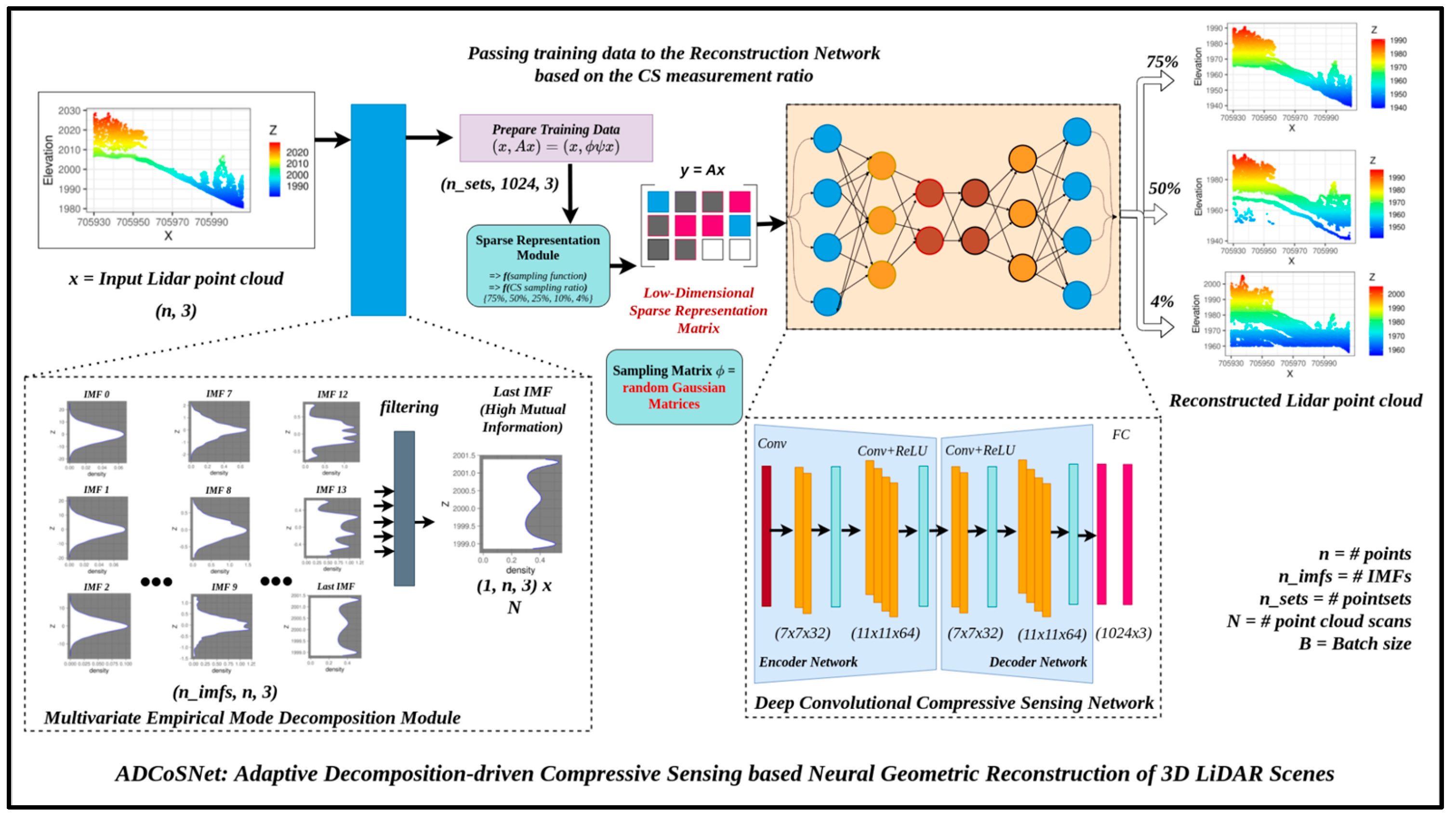
Figure 4.
Illustration of workflow for our proposed ADCoSNet for 3D Reconstruction of LiDAR Point Clouds. The Multivariate Empirical Mode Decomposition Module illustrates the filtering of last IMF having high mutual information. The filtered signal is passed to train the deep convolutional compressive sensing network for obtaining the sparse representations. Once the sparse representations are obtained, the network can subsequently be used to reconstruct the 3D LiDAR point clouds.
Figure 5.
Illustration showing the visualization of the original point set, first three IMFs, and last IMF for the selected Andrews 1 and Tahoe 1 datasets.
Figure 5.
Illustration showing the visualization of the original point set, first three IMFs, and last IMF for the selected Andrews 1 and Tahoe 1 datasets.
Figure 6.
(a) Variation in PSNR (dB) with the corresponding IMFs for the Andrews 1 dataset. (b) Relationship between PSNR in natural Log (Ln) scale and IMF for all the selected datasets.
Figure 6.
(a) Variation in PSNR (dB) with the corresponding IMFs for the Andrews 1 dataset. (b) Relationship between PSNR in natural Log (Ln) scale and IMF for all the selected datasets.
Figure 7.
Illustration showing the reconstructed point clouds using the proposed ADCoSNet for different CS ratios for the selected Andrews 1 and Andrews 2 test sites. (a) Original; (b) CS Ratio = 0.75; (c) CS Ratio = 0.50; (d) CS Ratio = 0.25; (e) CS Ratio = 0.10; (f) CS Ratio = 0.04.
Figure 7.
Illustration showing the reconstructed point clouds using the proposed ADCoSNet for different CS ratios for the selected Andrews 1 and Andrews 2 test sites. (a) Original; (b) CS Ratio = 0.75; (c) CS Ratio = 0.50; (d) CS Ratio = 0.25; (e) CS Ratio = 0.10; (f) CS Ratio = 0.04.
Figure 8.
Illustration showing the reconstructed point clouds using the proposed ADCoSNet for different CS ratios for the selected Tahoe 1, Tahoe 2 and Tahoe 3 test sites. (a) Original; (b) CS Ratio = 0.75; (c) CS Ratio = 0.50; (d) CS Ratio = 0.25; (e) CS Ratio = 0.10; (f) CS Ratio = 0.04.
Figure 8.
Illustration showing the reconstructed point clouds using the proposed ADCoSNet for different CS ratios for the selected Tahoe 1, Tahoe 2 and Tahoe 3 test sites. (a) Original; (b) CS Ratio = 0.75; (c) CS Ratio = 0.50; (d) CS Ratio = 0.25; (e) CS Ratio = 0.10; (f) CS Ratio = 0.04.
Figure 9.
Illustration of variation in (a) PSNR and (b) RMSE, with varying CS measurement ratios for the selected five samples from the Andrews and Tahoe dataset.
Figure 9.
Illustration of variation in (a) PSNR and (b) RMSE, with varying CS measurement ratios for the selected five samples from the Andrews and Tahoe dataset.
Figure 10.
Visualization of the generated Canopy Height Model (CHM) of the original and reconstructed 3D LiDAR point clouds using the proposed ADCoSNet for the Andrews 1 and Andrews 2 test site. (a) Original; (b) CS Ratio = 0.75; (c) CS Ratio = 0.50; (d) CS Ratio = 0.25; (e) CS Ratio = 0.10; (f) CS Ratio = 0.04.
Figure 11.
Visualization of the generated Canopy Height Model (CHM) of the original and reconstructed 3D LiDAR point clouds using the proposed ADCoSNet for the Tahoe 1, Tahoe 2, and Tahoe 3 test sites. (a) Original; (b) CS Ratio = 0.75; (c) CS Ratio = 0.50; (d) CS Ratio = 0.25; (e) CS Ratio = 0.10; (f) CS Ratio = 0.04.
Figure 12.
Visualization of the vertical elevation (2D cross-section) profiles of the subset of the original and reconstructed 3D LiDAR point clouds using the proposed ADCoSNet for the selected Andrews 1, Andrews 2, Tahoe 1, Tahoe 2, and Tahoe 3 test sites. (a) Original; (b) CS Ratio = 0.75; (c) CS Ratio = 0.50; (d) CS Ratio = 0.25; (e) CS Ratio = 0.10; (f) CS Ratio = 0.04.
Table 1.
Quantitative Results for Empirical Analysis of MEMD Derived Intrinsic Mode Functions (IMFs)—1st Four and Last Four Based on PSNR (Peak Signal To Noise Ratio), Mutual Information And Pearson’s Correlation Coefficient (r) for the Selected Samples.
Table 1.
Quantitative Results for Empirical Analysis of MEMD Derived Intrinsic Mode Functions (IMFs)—1st Four and Last Four Based on PSNR (Peak Signal To Noise Ratio), Mutual Information And Pearson’s Correlation Coefficient (r) for the Selected Samples.
| Original Sample/IMFs | Andrews 1 | Andrews 2 | Tahoe 1 | Tahoe 2 | Tahoe 3 |
|---|
| PSNR (dB) | MI | r | PSNR (dB) | MI | r | PSNR (dB) | MI | r | PSNR (dB) | MI | r | PSNR (dB) | MI | r |
|---|
| 1st IMF | 0.27 | 0.39 | 0.56 | 0.44 | 0.24 | 0.44 | 0.14 | 0.37 | 0.52 | 0.12 | 0.09 | 0.57 | 0.10 | 0.38 | 0.60 |
| 2nd IMF | 0.28 | 0.34 | 0.54 | 0.43 | 0.22 | 0.42 | 0.15 | 0.34 | 0.53 | 0.11 | 0.10 | 0.60 | 0.10 | 0.30 | 0.57 |
| 3rd IMF | 0.28 | 0.18 | 0.38 | 0.43 | 0.13 | 0.31 | 0.13 | 0.22 | 0.44 | 0.10 | 0.05 | 0.45 | 0.11 | 0.19 | 0.47 |
| 4th IMF | 0.28 | 0.07 | 0.28 | 0.44 | 0.07 | 0.21 | 0.14 | 0.13 | 0.33 | 0.12 | 0.02 | 0.32 | 0.11 | 0.09 | 0.32 |
| 4th Last IMF | 0.26 | 0.31 | 0.09 | 0.42 | 0.43 | 0.08 | 0.14 | 0.08 | 0.06 | 0.12 | 0.02 | 0.03 | 0.12 | 0.04 | 0.02 |
| 3rd Last IMF | 0.28 | 0.43 | 0.27 | 0.44 | 0.55 | 0.07 | 0.15 | 0.19 | 0.07 | 0.13 | 0.04 | 0.02 | 0.16 | 0.12 | 0.03 |
| 2nd Last IMF | 0.28 | 0.55 | 0.27 | 0.44 | 0.67 | 0.05 | 0.14 | 0.21 | 0.18 | 0.14 | 0.04 | 0.06 | 0.17 | 0.22 | 0.06 |
| Last IMF (Residue) | 35.7 | 0.35 | 0.22 | 36.2 | 0.99 | 0.66 | 50.6 | 0.38 | 0.36 | 45.5 | 0.09 | 0.08 | 50.0 | 0.30 | 0.09 |
Table 2.
Quantitative assessment of the reconstruction using our proposed ADCoSNet for the selected samples for different CS Measurement ratios based on the evaluation metrics—Peak Signal to Noise Ratio (PSNR in dB), Root Mean Square Error (RMSE), and Hausdorff distance (H.D.).
Table 2.
Quantitative assessment of the reconstruction using our proposed ADCoSNet for the selected samples for different CS Measurement ratios based on the evaluation metrics—Peak Signal to Noise Ratio (PSNR in dB), Root Mean Square Error (RMSE), and Hausdorff distance (H.D.).
| Sample Dataset/Evaluation Metric | CS Ratio = 0.75 | CS Ratio = 0.50 | CS Ratio = 0.25 | CS Ratio = 0.10 | CS Ratio = 0.04 |
|---|
| PSNR (dB) | RMSE | H.D. | PSNR (dB) | RMSE | H.D. | PSNR (dB) | RMSE | H.D. | PSNR (dB) | RMSE | H.D. | PSNR (dB) | RMSE | H.D. |
|---|
| Andrews 1 | 32.59 | 17.89 | 32.58 | 29.70 | 24.94 | 29.63 | 17.40 | 102.8 | 105.8 | 16.98 | 107.9 | 113.5 | 14.37 | 145.8 | 152.1 |
| Andrews 2 | 35.74 | 11.12 | 21.72 | 32.87 | 15.47 | 23.4 | 31.44 | 18.25 | 29.09 | 28.54 | 25.47 | 39.52 | 21.56 | 56.93 | 62.20 |
| Tahoe 1 | 48.96 | 7.21 | 11.19 | 42.95 | 14.39 | 20.83 | 40.77 | 18.50 | 28.79 | 37.84 | 25.90 | 31.32 | 36.14 | 31.52 | 36.85 |
| Tahoe 2 | 39.94 | 20.42 | 39.89 | 36.76 | 29.45 | 47.19 | 36.17 | 31.54 | 54.78 | 34.40 | 38.64 | 41.61 | 33.59 | 42.46 | 56.67 |
| Tahoe 3 | 48.35 | 7.69 | 11.45 | 42.64 | 14.84 | 18.26 | 40.75 | 18.45 | 22.25 | 37.66 | 26.33 | 28.79 | 35.43 | 34.03 | 40.82 |
Table 3.
Ablation Study for Multivariate Empirical Mode Decomposition as a basis transform for CS-based reconstruction using the proposed ADCoSNet framework (Overall PSNR in dB for Tahoe 1 with CS measurement ratio of 0.75).
Table 3.
Ablation Study for Multivariate Empirical Mode Decomposition as a basis transform for CS-based reconstruction using the proposed ADCoSNet framework (Overall PSNR in dB for Tahoe 1 with CS measurement ratio of 0.75).
| Proposed Architecture | Without MEMD | With MEMD |
|---|
| ADCoSNet | 40.94 dB | 48.96 dB |
| Disclaimer/Publisher’s Note: The statements, opinions and data contained in all publications are solely those of the individual author(s) and contributor(s) and not of MDPI and/or the editor(s). MDPI and/or the editor(s) disclaim responsibility for any injury to people or property resulting from any ideas, methods, instructions or products referred to in the content. |
© 2023 by the authors. Licensee MDPI, Basel, Switzerland. This article is an open access article distributed under the terms and conditions of the Creative Commons Attribution (CC BY) license (https://creativecommons.org/licenses/by/4.0/).


